Adaptive Fixed-Time Fractional-Order Terminal Sliding Mode Controller for Autonomous Underwater Vehicle Under External Disturbances

Highlights

What are the main findings?

• The proposed AFtFoNTSMC strategy ensures fixed-time convergence of tracking errors for AUVs, with the settling time bounded regardless of initial conditions, enhancing both transient and steady-state performance under external disturbances.
• A novel fractional-order non-singular terminal sliding manifold (FoNTSM) is designed, which effectively eliminates singularity issues and attenuates chattering while providing faster convergence compared to conventional integer-order approaches.

What are the implications of the main findings?

• The controller enhances robustness and precision in complex marine environments, enabling AUVs to perform demanding tasks (e.g., marine exploration, pipeline inspections) with predictable convergence times and reduced control input oscillations.
• By integrating fractional-order adaptive laws, the controller compensates for unknown disturbances without requiring prior knowledge of their bounds, reducing dependence on precise dynamic modeling and expanding AUVs’ applicability in real-world scenarios with uncertain conditions.

Abstract

This paper proposes an adaptive fixed-time fractional-order non-singular terminal sliding mode control (AFtFoNTSMC) strategy to enhance the trajectory tracking performance of autonomous underwater vehicles (AUVs) under external disturbances. A novel fractional-order non-singular terminal sliding mode (FoNTSM) control strategy was developed, which effectively resolves singularity problems and attenuates chattering. To compensate for unknown disturbances, a fractional-order adaptive law was developed, which enhances system robustness without requiring prior knowledge of disturbance bounds. Building upon fixed-time stability theory, the proposed controller ensures that tracking errors converge to equilibrium within a predetermined settling time, independent of initial conditions. Lyapunov stability analysis rigorously proved the system’s fixed-time stability and provided an upper bound for the convergence time. Comparative simulations demonstrated that the AFtFoNTSMC outperforms conventional methods in terms of tracking accuracy, chattering suppression, and disturbance rejection, validating its effectiveness and superiority.

1. Introduction

In recent years, AUVs have become indispensable tools for a wide range of maritime applications, from deep-sea exploration and seabed mapping to critical infrastructure inspections, environmental monitoring, and defense operations [1]. The effective execution of these complex missions fundamentally depends on the vehicle’s ability to follow a predefined trajectory with high precision. However, the development of robust control systems for AUVs is particularly challenging due to their inherent underactuated configuration, strong nonlinear dynamics, and significant system uncertainties [2]. These challenges are further compounded by the harsh and unpredictable ocean environment, where factors such as currents, waves, and variable buoyancy continuously disturb the vehicle’s motion. Consequently, there is a pressing need for advanced trajectory tracking controllers that are not only highly precise but also exhibit strong robustness and rapid convergence to ensure reliable and optimal performance under such demanding conditions [3].

Among the existing control methods, sliding mode control (SMC) gas high robustness against model parameter variations and external disturbances in nonlinear systems. The essence of SMC lies in maintaining the system state on a specifically designed sliding surface, ensuring robust and predictable dynamic behavior. Based on these good features, sliding mode control has been widely used in the trajectory tracking of AUVs; for example, see [4,5,6,7,8]. When AUVs execute a trajectory tracking mission, finite-time convergence is always highly important. While linear SMC fails to meet this requirement, terminal sliding mode control (TSMC) [9] resolves this limitation through nonlinear sliding surfaces, ensuring robust stabilization. Nevertheless, conventional TSMC still faces challenges with singularity issues and insufficient convergence speed. To address these limitations, ref. [10] proposed fast non-singular terminal integral sliding mode control (FNITSM), which avoids the singularity problem and ensures rapid transient convergence distant and near to the equilibrium point, significantly reducing the convergence time. Because of the model uncertainties and external disturbances encountered by AUVs, the aforementioned methods are unable to ensure satisfactory control performance. To mitigate these challenges, a growing number of control strategies are incorporating adaptive strategies to improve the closed-loop tracking performance [11,12]. In ref. [13], an adaptive fast nonsingular integral terminal sliding mode control (AFNITSMC) was proposed for 3D trajectory tracking of unmanned underwater vehicles under model uncertainties and disturbances. The method has global finite-time convergence of tracking errors within small bounded regions. However, a key limitation of finite-time sliding mode control is its dependence on initial system states for the convergence time. This drawback affects the overall tracking performance and restricts the applicability of finite-time control strategies in real-world scenarios.

To address the aforementioned challenges, a series of fixed-time convergence theorems have been developed, which have garnered substantial research interest. These theorems ensure that the convergence of system states are uniformly bounded and that the upper limit of the convergence time is independent of the initial states [14,15]. Through use of the fixed-time integral sliding mode manifold, a continuous fixed-time disturbance observer was developed in ref. [16] to estimate the unknown external disturbances. This proposed control strategy guarantees that the tracking errors of the underactuated AUV converge to a bounded region in a predetermined fixed time. In ref. [17], a fixed-time terminal sliding mode controller (FtSMC) integrated with a neural network observer was introduced to address the trajectory tracking control challenge for AUVs subject to time-varying external disturbances. It should be emphasized that the prevailing TSMC designs are predominantly restricted to the utilization of integer-order (IO) differentiators or IO integrators. This inherent constraint frequently leads to diminished control accuracy and exacerbated system jitter, thereby impeding overall performance optimization.

Fractional calculus has increasingly garnered significant interest in a multitude of engineering applications [18,19]. In contrast to conventional IO designs, fractional-order (FO) control systems possess a more extensive range of adjustable degrees of freedom. This increased flexibility effectively bolsters robustness against model uncertainties and external disturbances while mitigating the chattering with sliding mode control [20,21]. Moreover, the FO scheme can leverage the memory and hereditary properties of fractional-order operators to enhance the smoothness and continuity of control behavior [22], thereby refining overall system performance. To facilitate high-speed operations of permanent magnet synchronous motors, an adaptive super-twisting nonlinear fractional-order PID sliding mode strategy with an extended state observer (ESO) was proposed in ref. [23]. In ref. [24], the authors introduced an adaptive fractional-order sliding mode controller designed to effectively control and stabilize a nonlinear, disturbance-affected robotic manipulator. To improve power quality, a fixed-time fractional-order sliding mode controller has been developed for the permanent magnet synchronous generator (PMSG) within wind turbine systems [25]. However, to the best of the authors’ knowledge, the application of fractional-order fixed-time sliding mode control to the trajectory tracking of underactuated AUVs remains an unexplored area in the existing literature. This research gap is particularly significant given two critical aspects: First, the inherent nonlinearity, strong coupling, and underactuated characteristics of AUVs pose substantial challenges for conventional control methods. Second, the intricate and unpredictable nature of marine environments, characterized by time-varying ocean currents, wave disturbances, and measurement uncertainties, further exacerbates the control difficulties. The conventional sliding mode control based on IO calculus, while offering certain robustness, exhibits three major limitations in this context: (1) finite-time convergence that depends on initial system states, (2) inherent chattering phenomenon, and (3) inadequate control accuracy in handling uncertainty and disturbances. Consequently, there is an urgent need to develop an advanced fixed-time fractional-order control strategy for AUV trajectory tracking systems, particularly in complex marine operational scenarios. This necessity forms the core inspiration behind the research described within this paper.

Based on the foregoing discussion and to address the identified research gaps, the paper proposes a novel adaptive fixed-time fractional-order non-singular terminal sliding mode controller for underactuated AUVs. The major contributions of this work are systematically highlighted as follows:

1.

In this paper, a novel AFtFoNTSMC control method is proposed for underactuated AUVs. Different from the asymptotically stable or finite-time stable approach in [8,13], based on fixed-time stability theory, the proposed strategy was developed that enhances the transient and steady-state performance of AUV trajectory tracking. Notably, the upper bound of the convergence time for tracking errors can be preset independently of the system’s initial state, ensuring predictable and robust performance under diverse operating conditions.

2.

A FoNTSM surface with enhanced tracking performance was designed. Unlike the conventional fixed-time sliding mode approaches in [26], the proposed FoNTSM, built upon fractional-order calculus, avoids potential singularity issues and attenuates chattering more simply and efficiently, and there is no non-differentiability problem commonly associated with piecewise functions. Moreover, this sliding manifold guarantees fast convergence with a bounded and predetermined maximum settling time, thereby providing improved operational predictability for AUV tracking motion.

3.

To address the challenges arising from external disturbances in marine environments, a novel fractional-order adaptive law was developed. This method eliminates the need for exact prior knowledge of disturbance bounds and enables effective compensation for thrusters, thereby substantially improving the disturbance rejection capability in this proposed control strategy.

4.

Two simulations were conducted under various ocean disturbances and operating scenarios. Numerous visualized results and quantitative data demonstrate the robustness, effectiveness, and superiority of the proposed AFtFoNTSMC method.

The remainder of this paper is organized as follows. The problem formulation is presented in Section 2. The methodology design and theoretical analysis of AFtFoNTSMC are elaborated in detail in Section 3. Section 4 provides simulation verification and comparison studies. Section 5 concludes this article.

2. Problem Formulation and Preliminaries

2.1. Lemmas and Definitions

Definition 1

([27]). Within the domain of fractional calculus, the Riemann–Liouville (RL) formulation is widely utilized. The subsequent expression delineates the Riemann–Liouville’s fractional-order derivative of the order β of the continuous-time function z(t).

$${}_a\mathcal{D}_t^{\beta }z\left(t\right)={\displaystyle \frac{{\mathrm{d}}^{\beta }z\left(t\right)}{\mathrm{d}{t}^{\beta }}}={\displaystyle \frac{1}{\Gamma (1-\beta )}}{\displaystyle \frac{\mathrm{d}}{\mathrm{d}t}}{\int }_a^t{\displaystyle \frac{z\left(\tau \right)}{{(t-\tau )}^{\beta }}}\mathrm{d}\tau$$

(1)

where D is the fractional-order operator, β is the fractional order, and a and t denote the limitation of the operation. The gamma function $\Gamma (.)$ based on Euler can be defined as

$$\Gamma \left(\beta \right)={\int }_0^{\infty }{\mathrm{e}}^{-t}{t}^{\beta -1}\mathrm{d}t$$

(2)

Property 1

([28]). The following equation represents the relationship that holds for the Riemann-Liouville fractional-order derivative

$${\displaystyle \frac{d^n}{d{t}^n}}{D}^{\alpha }f\left(t\right)=D^{n+\alpha }f\left(t\right)=D^{\alpha }{\displaystyle \frac{d^n}{d{t}^n}}f\left(t\right)$$

(3)

$$D^{\alpha }[af\left(t\right)+bg\left(t\right)]=a{D}^{\alpha }f\left(t\right)+b{D}^{\alpha }g\left(t\right)$$

(4)

Lemma 1

([28]). Consider the nonlinear systems

$$\left\{\begin{array}{c}\dot{x}\left(t\right)=f\left(x\left(t\right)\right)\hfill \\ x\left(0\right)=x_0\hfill \end{array}\right.$$

(5)

where x denotes the state variable, and $f\left(x\right(t\left)\right)$ represents a continuous and nonlinear function. To ensure fixed-time stability and convergence, the Lyapunov function $V\left(x\right)$ must satisfy the following conditions

$$\begin{array}{cc}\hfill \left(i\right)V\left(x\right)& =0\iff x=0\hfill \end{array}$$

(6)

$$\begin{array}{cc}\hfill \left(ii\right)\dot{V}\left(x\right)& \le -{\kappa }_1{V}^{{\phi }_1}\left(x\right)-{\kappa }_2{V}^{{\phi }_2}\left(x\right)\hfill \end{array}$$

(7)

where ${\kappa }_1$ and ${\kappa }_2$ are positive numbers, $0<{\phi }_1<1$, and ${\phi }_2>1$. Then the dynamic system can be considered to be fixed-time stable. The convergence time can be determined by the following

$$\begin{array}{c}\hfill T\le {\displaystyle \frac{1}{{\kappa }_1\left(1-{\phi }_1\right)}}+{\displaystyle \frac{1}{{\kappa }_2\left({\phi }_2-1\right)}}\end{array}$$

(8)

Lemma 2

([29]). For system (5), if the Lyapunov function $V\left(x\right)$ satisfies the following conditions

$$\begin{array}{cc}\hfill \left(i\right)V\left(x\right)& =0\iff x=0\hfill \end{array}$$

(9)

$$\begin{array}{cc}\hfill \left(ii\right)D^{\alpha }V\left(x\right)& \le -a{V}^{\beta }\left(x\right)-b{V}^{\gamma }\left(x\right)\hfill \end{array}$$

(10)

where a and b are positive numbers, and $0<\gamma <1<\beta <\alpha +1$, $0<\gamma <\alpha <1<\beta$. Subsequently, the dynamic system can be deemed fixed-time stable. Time to convergence can be calculated as

$$T\left(x_0\right)\le {\left(-{\displaystyle \frac{\Gamma (1-\beta )\Gamma (1+\alpha )}{a\Gamma (1+\alpha -\beta )}}\right)}^{{\displaystyle \frac{1}{\alpha }}}+{\left({\displaystyle \frac{\Gamma (1-\gamma )\Gamma (1+\alpha )}{b\Gamma (1+\alpha -\gamma )}}\right)}^{{\displaystyle \frac{1}{\alpha }}}$$

(11)

Lemma 3

([24]). With ${\epsilon }_1,{\epsilon }_2,{\epsilon }_3,\dots ,{\epsilon }_n>0$, the inequalities are given as

$$\sum _{i=1}^n{\left|{\epsilon }_i\right|}^{1+\eta }\ge {\left(\sum _{i=1}^n{\left|{\epsilon }_i\right|}^2\right)}^{{\displaystyle \frac{1+\eta }{2}}},\mathit{for}0<\eta <1$$

(12)

$$\sum _{i=1}^n{\left|{\epsilon }_i\right|}^{\eta }\ge n^{1-\eta }{\left(\sum _{i=1}^n\left|{\epsilon }_i\right|\right)}^{\eta },\mathit{for}\eta >1$$

(13)

Lemma 4

([30]). For all time instances $t\ge 0$, the following inequality can be held:

$$D^{\alpha }\left({\displaystyle \frac{1}{2}}{x}^{\top }\left(t\right)Qx\left(t\right)\right)\le x^{\top }\left(t\right)Q{D}_t^{\alpha }x\left(t\right)$$

(14)

where $\mathbf{Q}\in {\Re }^{n\times n}$ is a symmetric positive definite matrix of gain.

2.2. Model of Underactuated AUV

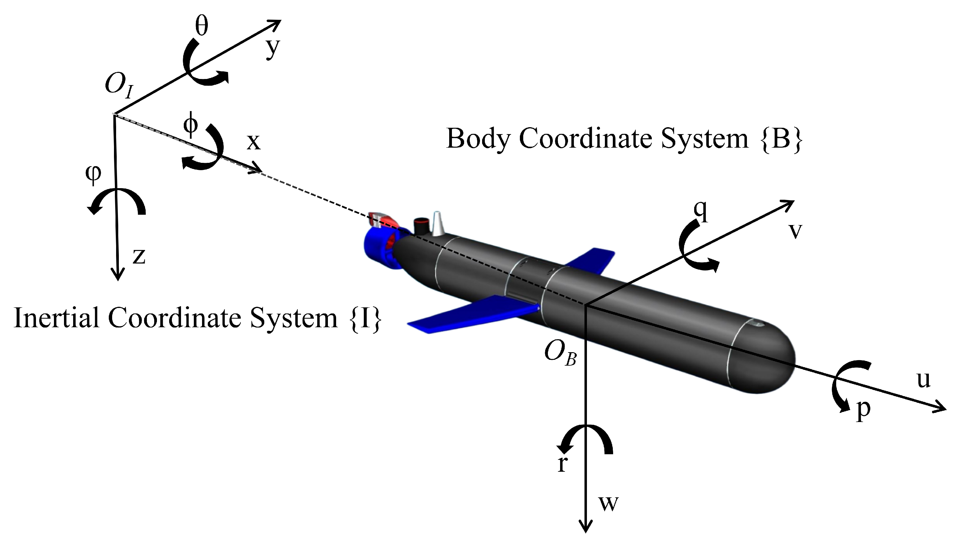
In order to determine the six degree of freedom nonlinear motion equation of an AUV, two reference coordinate systems are usually defined: one is the inertial frame, which is considered fixed on the earth, and the other is a body-fixed frame, which is considered fixed on the AUV and moves with it. As shown in Figure 1, the inertial coordinate system and body coordinate system are usually described by two vectors, $\mathsf{\eta }={[x,y,z,\varphi ,\theta ,\psi ]}^T$ and $\mathit{v}={[u,v,w,p,q,r]}^T$ respectively. $x,y,z\in \Re$ and $\varphi ,\theta ,\psi \in \Re$ (roll, pitch, and yaw) denote the position and attitude information respectively in inertial frames, which have a strong association with linear velocities $u,v,w\in \Re$ (surge, sway, and heave velocities) and angular velocities $p,q,r\in \Re$ in the body-fixed frame. The model considered in the research is the hybrid AUV2000, as referenced in [31]. To establish the relationship between the physical quantities in the two coordinate systems, the coordinate transformation matrix is employed as follows:

$$\dot{\mathsf{\eta }}=\mathit{J}\left(\mathsf{\eta }\right)\mathit{v}$$

(15)

where $\mathit{J}\left(\mathsf{\eta }\right)\in {\Re }^{6\times 6}$ is the Jacobian matrix, defined as

$$\mathit{J}\left(\mathsf{\eta }\right)=\left[\begin{array}{cc}{\mathit{J}}_1\left(\mathsf{\eta }\right)& {\mathbf{0}}_{3\times 3}\\ {\mathbf{0}}_{3\times 3}& {\mathit{J}}_2\left(\mathsf{\eta }\right)\end{array}\right]$$

(16)

where $0_{3\times 3}\in {\Re }^{3\times 3}$ denotes the zero matrix, and ${\mathit{J}}_1\left(\mathsf{\eta }\right)\in {\Re }^{3\times 3}$ and ${\mathit{J}}_2\left(\mathsf{\eta }\right)\in {\Re }^{3\times 3}$ are represented as follows:

$${\mathit{J}}_1\left(\mathsf{\eta }\right)=\left[\begin{array}{ccc}c\left(\psi \right)c\left(\theta \right)& c\left(\psi \right)s\left(\theta \right)s\left(\varphi \right)-c\left(\psi \right)c\left(\varphi \right)& s\left(\psi \right)s\left(\varphi \right)+c\left(\psi \right)c\left(\varphi \right)s\left(\theta \right)\\ s\left(\psi \right)c\left(\theta \right)& c\left(\psi \right)c\left(\varphi \right)+c\left(\psi \right)s\left(\theta \right)s\left(\varphi \right)& s\left(\psi \right)c\left(\varphi \right)s\left(\theta \right)-c\left(\psi \right)s\left(\varphi \right)\\ -s\left(\theta \right)& c\left(\theta \right)s\left(\varphi \right)& c\left(\theta \right)c\left(\varphi \right)\end{array}\right]$$

(17)

$${\mathit{J}}_2\left(\mathsf{\eta }\right)=\left[\begin{array}{ccc}1& t\left(\theta \right)s\left(\varphi \right)& t\left(\theta \right)c\left(\varphi \right)\\ 0& c\left(\varphi \right)& -s\left(\varphi \right)\\ 0& s\left(\varphi \right)/c\left(\theta \right)& c\left(\varphi \right)/c\left(\theta \right)\end{array}\right]$$

(18)

where $s(.), c(.)$ and $t(.)$ denote $sin(.), cos(.)$ and $tan(.)$ respectively.

Assumption 1

([32]). Due to restoring forces, the pitch angle θ of an AUV in practical applications is limited to $\left|\theta \right|\le {\theta }_{max}<\pi /2$ to prevent the singularity problem in which ${\theta }_{max}>0$. Therefore ${\mathit{J}}_2\left(\mathsf{\eta }\right)$ is non-exotic.

Assumption 2

([2]). The coordinate transformation matrix $\mathit{J}\left(\mathsf{\eta }\right)$ and its inverse matrix ${\mathit{J}}^{-\mathbf{1}}\left(\mathsf{\eta }\right)$ are invertible and bounded. There exists two known constant $\overline{\mathit{J}}>0$ and ${\overline{\mathit{J}}}_{\mathit{inv}}>0$ such that $∥\mathit{J}\left(\mathsf{\eta }\right)∥⩽\overline{\mathit{J}}$ and $∥{\mathit{J}}^{-\mathbf{1}}\left(\mathsf{\eta }\right)∥⩽{\overline{\mathit{J}}}_{\mathit{inv}}$.

Assumption 3

([2]). There are undetermined constants $\overline{\mathit{M}}\in {\Re }^{+}, \overline{\mathit{C}}\left(\mathit{v}\right)\in {\Re }^{+}$, $\overline{\mathit{D}}\left(\mathit{v}\right)\in {\Re }^{+}$ and $\overline{\mathit{g}}\left(\mathsf{\eta }\right)\in {\Re }^{+}$, which ensure that the parameters within the kinetic model adhere to the inequalities $∥\mathit{M}∥⩽\overline{\mathit{M}},∥\mathit{C}\left(\mathit{v}\right)∥⩽\overline{\mathit{C}}\left(\mathit{v}\right),∥\mathit{D}\left(\mathit{v}\right)∥⩽\overline{\mathit{D}}\left(\mathit{v}\right)$ and $∥\mathit{g}\left(\mathsf{\eta }\right)∥⩽\overline{\mathit{g}}\left(\mathsf{\eta }\right)$.

The AUV’s dynamic model, formulated within a body fixed coordinate system, is expressed through the following equation

$$\mathit{M}\dot{\mathit{v}}+\mathit{C}\left(\mathit{v}\right)\mathit{v}+\mathit{D}\left(\mathit{v}\right)\mathit{v}+\mathit{g}\left(\mathsf{\eta }\right)+{\mathsf{\tau }}_d={\mathsf{\tau }}_v$$

(19)

where $\mathit{M}\in {\Re }^{6\times 6}$ is the inertia matrix including the additional mass, $\mathit{C}\left(\mathit{v}\right)\in {\Re }^{6\times 6}$ is the rigid body Coriolis and centripetal matrix, $\mathit{D}\left(\mathit{v}\right)\in {\Re }^{6\times 6}$ denotes the matrix with damping terms, $\mathit{g}\left(\mathsf{\eta }\right)\in {\Re }^6$ denotes the restoring force vector (gravity and buoyancy), ${\mathsf{\tau }}_{\mathit{d}}$ denotes the vector of time-varying external disturbances, and ${\mathsf{\tau }}_{\mathit{v}}$ denotes the vector of generalized thrusts.

In real-world scenarios, it is often impractical to ascertain the precise dynamics of AUVs. Consequently, the parameter matrices within the AUVs’ dynamic model (19) is effectively partitioned into two distinct components: nominal term, which represents the known and expected aspects, and the uncertain term, which summarizes the unknown and variable elements. Define the parameter errors as

$$\begin{array}{cc}\hfill \tilde{\mathit{M}}& =\mathit{M}-\widehat{\mathit{M}}\hfill \\ \hfill \tilde{\mathit{C}}\left(\mathit{v}\right)& =\mathit{C}\left(\mathit{v}\right)-\widehat{\mathit{C}}\left(\mathit{v}\right)\hfill \\ \hfill \tilde{\mathit{D}}\left(\mathit{v}\right)& =\mathit{D}\left(\mathit{v}\right)-\widehat{\mathit{D}}\left(\mathit{v}\right)\hfill \\ \hfill \tilde{\mathit{g}}\left(\mathsf{\eta }\right)& =\mathit{g}\left(\mathsf{\eta }\right)-\widehat{\mathit{g}}\left(\mathsf{\eta }\right)\hfill \end{array}$$

(20)

where $\widehat{\mathit{M}}$, $\widehat{\mathit{C}}\left(\mathit{v}\right)$, $\widehat{\mathit{D}}\left(\mathit{v}\right)$, and $\widehat{\mathit{g}}\left(\mathsf{\eta }\right)$ represent the nominal terms, while $\tilde{\mathit{M}}$, $\tilde{\mathit{C}}\left(\mathit{v}\right)$, $\tilde{\mathit{D}}\left(\mathit{v}\right)$, and $\tilde{\mathit{g}}\left(\mathsf{\eta }\right)$ represent the uncertain terms. Then Formula (19) can be rewritten as

$$(\widehat{\mathit{M}}+\tilde{\mathit{M}})\dot{\mathit{v}}+(\widehat{\mathit{C}}\left(\mathit{v}\right)+\tilde{\mathit{C}}\left(\mathit{v}\right))\mathit{v}+(\widehat{\mathit{D}}\left(\mathit{v}\right)+\tilde{\mathit{D}}\left(\mathit{v}\right))\mathit{v}+(\widehat{\mathit{g}}\left(\mathsf{\eta }\right)+\tilde{\mathit{g}}\left(\mathsf{\eta }\right))+{\mathsf{\tau }}_d={\mathsf{\tau }}_v$$

(21)

Define the integrated system uncertainty ${\mathsf{\tau }}_{d\eta }$ as follows:

$${\mathsf{\tau }}_{d\eta }=-\tilde{\mathit{M}}\dot{\mathit{v}}-\tilde{\mathit{C}}\left(\mathit{v}\right)\mathit{v}-\tilde{\mathit{D}}\left(\mathit{v}\right)\mathit{v}-\tilde{\mathit{g}}\left(\mathsf{\eta }\right)-{\mathsf{\tau }}_d$$

(22)

dynamic model (21) can be represented as follows:

$$\widehat{\mathit{M}}\dot{\mathit{v}}+\widehat{\mathit{C}}\left(\mathit{v}\right)\mathit{v}+\widehat{\mathit{D}}\left(\mathit{v}\right)\mathit{v}+\widehat{\mathit{g}}\left(\mathsf{\eta }\right)={\mathsf{\tau }}_v+{\mathsf{\tau }}_{d\eta }$$

(23)

Assumption 4

([32]). A positive constant ${\overline{\mathsf{\tau }}}_{\mathit{d}}$ satisfying $∥{\mathsf{\tau }}_d∥<{\overline{\mathsf{\tau }}}_{\mathit{d}}$ indicates that the unknown external disturbance vector ${\mathsf{\tau }}_{\mathit{d}}$ is upper bounded.

From Assumption 4, the following assumption can be obtained.

Assumption 5

([33]). If the AUVs encounters uncertainties and disturbances of a non-severe nature and pursues a desired trajectory that is not overly complex leading to infrequent saturation of the vehicle’s thruster forces, then ${\mathsf{\tau }}_{d\eta }$ can be constrained within bounds expressed by the following formulation:

$$\parallel {\mathsf{\tau }}_{d\eta }\parallel <{\lambda }_0+{\lambda }_1\parallel \mathit{v}\parallel +{\lambda }_2{\parallel \mathit{v}\parallel }^2$$

(24)

where ${\lambda }_i(i=0,1,2)$ represent unknown positive constants.

Remark 1.

According to the formulation $\mathit{g}\left(\mathsf{\eta }\right)$ presented in [34], $\mathit{g}\left(\mathsf{\eta }\right)$ is exclusively connected to η through the trigonometric representation of Euler angles, indicating that it is justified to assume there exists an unknown upper bound for η.

Remark 2.

The AUV2000 is an underactuated system specifically designed to operate without the use of a thruster. Its input force vector,$\tau =[T_{prop},0,0,y_G,x_G,{\delta }_R]$, controls four degrees of freedom, which including roll, pitch, yaw, surge. Here, $T_{prop}$ is the propeller force responsible for surge locomotion, while ${\delta }_R$ denotes the rudder angle. Additionally, $x_G$ and $y_G$ correspond to the coordinates of the AUV’s center of gravity, which is dynamically adjusted via a counterweight mechanism.

2.3. Control Objective

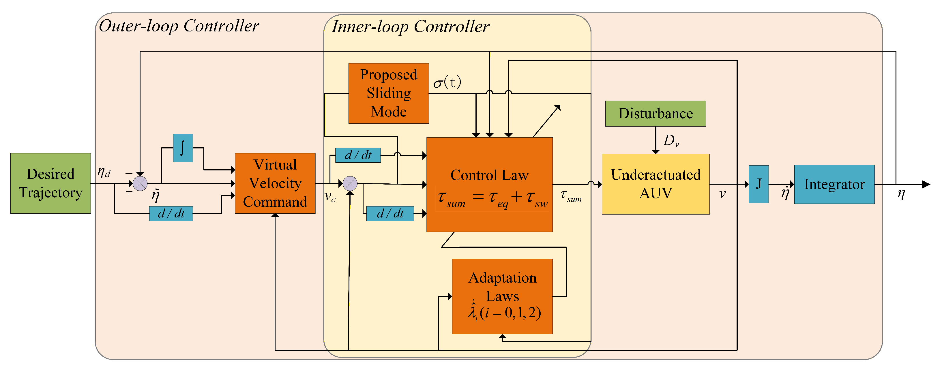
To achieve the control objective, a dual closed-loop controller was designed to drive the underactuated AUV to the desired trajectory, with strong robustness against the vehicle’s dynamic uncertainties and time-varying external disturbances.This controller can be decomposed into two components: an outer position kinematic controller ${\mathit{v}}_{\mathbf{c}}$ and an inner velocity dynamic controller ${\mathsf{\tau }}_{\mathit{v}}$. These are depicted as follows:

(i) Kinematic control: Given a desired three-dimensional reference and the dynamic model (15), an integral sliding mode was designed to obtain the virtual velocity inputs for dynamic control, with the position tracking error $\tilde{\mathsf{\eta }}$ asymptotically converging to an arbitrarily small neighborhood of zero.

(ii) Dynamic control: Given the virtual velocity $v_r$ and the dynamic model (23), an AFtFoNTSMC control strategy was designed to generate the control laws $T_{prop}$, $y_G$, $x_G$, and ${\delta }_R$ to guarantee that the velocity tracking error $\tilde{\mathit{v}}$ asymptotically converges to an arbitrarily small neighborhood of zero, with the upper convergence time being limited and predetermined.

3. Main Results

This section described the AFtFoNTSMC control strategy for improving the control performance of underactuated AUVs. Initially, an integral terminal sliding mode is utilized to estimate the virtual velocity command. Subsequently, based on the fixed-time theorem, a novel fractional-order sliding surface, along with fractional-order reaching law, is described. Then, to estimate the upper bounds of the unknown integrated disturbance, a fractional-order adaptive law is proposed. In addition, the stability of the aforementioned methods is investigated through Lyapunov theorem analysis. The specific schematic diagram of the proposed dual closed-loop control system for AUV trajectory tracking is depicted in Figure 2.

3.1. Outer-Loop Controller

The outer loop is configured to design a virtual velocity that guarantees precise position tracking, which subsequently serves as a virtual input for the velocity tracking in the inner loop. For a desired reference trajectory with time-varying ${\mathsf{\eta }}_d\in {\Re }^6$, designate $\tilde{\mathsf{\eta }}=\mathsf{\eta }-{\mathsf{\eta }}_d$ as the position tracking errors. With Equation (15), the following can be derived:

$$\dot{\tilde{\mathsf{\eta }}}=\mathit{J}\left(\mathsf{\eta }\right)\mathit{v}-{\dot{\mathsf{\eta }}}_d$$

(25)

Assumption 6.

The desired reference trajectory ${\mathsf{\eta }}_{\mathit{d}}={[x_d,y_d,z_d,{\varphi }_d,{\theta }_d,{\psi }_d]}^T$ and its time derivative ${\dot{\mathsf{\eta }}}_{\mathit{d}}={[{\dot{x}}_d,{\dot{y}}_d,{\dot{z}}_d,{\dot{\varphi }}_d,{\dot{\theta }}_d,{\dot{\psi }}_d]}^T$ are both constrained within finite bounds. Each corresponding element of these vectors constitutes a continuous and smooth function.

The integral sliding variable ${\mathit{S}}_{\mathsf{\eta }}$ for the outer loop is defined as

$${\mathit{S}}_{\mathsf{\eta }}=\tilde{\mathsf{\eta }}+{\mathsf{\kappa }}_{\mathsf{\eta }}{\int }_0^t\tilde{\mathsf{\eta }}\left(\tau \right)d\tau$$

(26)

where ${\mathsf{\kappa }}_{\mathsf{\eta }}=diag({\kappa }_{\eta 1},\dots ,{\kappa }_{\eta 6})$ denotes the positive control parameter. By taking the time derivative of Equation (26) and substituting Equation (25) into the result, the following can be obtained:

$$\dot{{\mathit{S}}_{\mathsf{\eta }}}=\mathit{J}\left(\mathsf{\eta }\right)\mathit{v}-{\dot{\mathsf{\eta }}}_d+{\mathsf{\kappa }}_{\mathsf{\eta }}\tilde{\mathsf{\eta }}\left(t\right)$$

(27)

Then, the velocity virtual commands ${\mathit{v}}_{\mathbf{c}}$ can be defined as

$${\mathit{v}}_{\mathbf{c}}={\mathit{J}}_{\left(\mathsf{\eta }\right)}^{-\mathbf{1}}({\dot{\mathsf{\eta }}}_{\mathit{d}}-{\mathsf{\kappa }}_{\mathsf{\eta }}\tilde{\mathsf{\eta }}-{\mathsf{\kappa }}_{\mathit{s}}{\mathit{S}}_{\mathsf{\eta }}-{\mathsf{\rho }}_{\mathit{s}}\mathbf{tanh}\left({\mathit{S}}_{\mathsf{\eta }}/{\mathsf{\Omega }}_{\mathit{s}}\right))$$

(28)

where ${\mathsf{\kappa }}_{\mathit{s}}=diag({\kappa }_{s1},\dots ,{\kappa }_{s6})$ and ${\mathsf{\rho }}_{\mathit{s}}=diag({\rho }_{s1},\dots ,{\rho }_{s6})$ are positive control parameters needed to be design, ${\mathsf{\Omega }}_{\mathit{s}}={[{\mathsf{\Omega }}_{s1},\dots ,{\mathsf{\Omega }}_{s6}]}^T$ represent the thickness of boundary layer. Now consider the following Lyapunov control function

$${\mathit{V}}_{\mathbf{1}}={\displaystyle \frac{1}{2}}{\mathit{S}}_{\mathsf{\eta }}^{\mathit{T}}{\mathit{S}}_{\mathsf{\eta }}$$

(29)

Taking the time derivative of Equation (29) and substituting Equations (27) and (28) into it, one obtains

$$\begin{array}{cc}\hfill \dot{{\mathit{V}}_{\mathbf{1}}}& ={\mathit{S}}_{\mathsf{\eta }}^{\mathit{T}}{\dot{\mathit{S}}}_{\mathsf{\eta }}\hfill \\ \hfill & ={\mathit{S}}_{\mathsf{\eta }}^{\mathit{T}}(\mathit{J}\left(\mathsf{\eta }\right)\left({\mathit{J}}_{\left(\mathsf{\eta }\right)}^{-\mathbf{1}}({\dot{\mathsf{\eta }}}_{\mathit{d}}-{\mathsf{\kappa }}_{\mathsf{\eta }}\tilde{\mathsf{\eta }}-{\mathsf{\kappa }}_{\mathit{s}}{\mathit{S}}_{\mathsf{\eta }}-{\mathsf{\rho }}_{\mathit{s}}\mathbf{tanh}\left({\mathit{S}}_{\mathsf{\eta }}/{\mathsf{\Omega }}_{\mathit{s}}\right))\right)-{\dot{\mathsf{\eta }}}_d+{\mathsf{\kappa }}_{\mathsf{\eta }}\tilde{\mathsf{\eta }}\left(t\right))\hfill \\ \hfill & =-{\mathsf{\kappa }}_{\mathit{s}}{\mathit{S}}_{\mathsf{\eta }}^{\mathit{T}}{\mathit{S}}_{\mathsf{\eta }}-{\mathsf{\rho }}_{\mathit{s}}{\mathit{S}}_{\mathsf{\eta }}^{\mathit{T}}\mathbf{tanh}({\mathit{S}}_{\mathsf{\eta }}/{\mathsf{\Omega }}_{\mathit{s}})\hfill \end{array}$$

(30)

Given that $\dot{{\mathit{V}}_{\mathbf{1}}}<0$, it indicates that the designed Lyapunov function ${\mathit{V}}_{\mathbf{1}}$ is negative semi-definite. Therefore, the error variables ${\mathit{S}}_{\mathsf{\eta }}$ and $\tilde{\mathsf{\eta }}$ can converge to zero.

Remark 3.

In (28), the specific structure $-{\mathsf{\kappa }}_{\mathit{s}}{\mathit{S}}_{\mathsf{\eta }}-{\mathsf{\rho }}_{\mathit{s}}\mathbf{tanh}({\mathit{S}}_{\mathsf{\eta }}/{\mathsf{\Omega }}_{\mathit{s}})$ serves as the reaching law component. The hyperbolic tangent function $\mathbf{tanh}\mathbf{(}\mathbf{.}\mathbf{)}$ is employed to approximate the signum function, thereby effectively mitigating control chattering and ensuring a smooth virtual command signal. This design is essential for maintaining the stability of the subsequent dynamic control loop.

Remark 4.

In the practical application, target trajectory is defined as a smooth and continuous function, guaranteeing the continuity of the control law and thereby validating the practicality of Assumption 6.

3.2. Proposed FoNTSM Manifold

Due to the complex and unpredictable nature of marine environments, conventional TSMC with IO calculus for AUVs exhibits serious chattering phenomena, leading to insufficient control accuracy in practical applications. To address this issue, a novel fractional-order non-singular terminal sliding surface was designed in this study.Compared with [13], this design can achieve higher estimation tracking accuracy for AUVs. The sliding manifold was designed as follows:

$$\mathsf{\sigma }\left(\mathit{t}\right)=D^{-\alpha }\left(\tilde{\mathit{e}}\left(\mathit{t}\right)\right)+{\mathit{X}}_{\mathbf{1}}{D}^{-\alpha -1}\left({sig}^{{\displaystyle \frac{m_1}{m_2}}}\left(\tilde{\mathit{e}}\left(\mathit{t}\right)\right)\right)+{\mathit{X}}_{\mathbf{2}}{D}^{-\alpha -1}\left({sig}^{{\displaystyle \frac{p_1}{p_2}}}\left(\tilde{\mathit{e}}\left(\mathit{t}\right)\right)\right)$$

(31)

where $\mathsf{\sigma }\left(\mathit{t}\right)={[{\sigma }_1,{\sigma }_2,\dots ,{\sigma }_n]}^T\in {\Re }^n$ is the proposed sliding surface; $\alpha \in (0,1)$ denotes fractional order; and $\tilde{\mathit{e}}\left(\mathit{t}\right)=\mathit{v}-{\mathit{v}}_{\mathbf{c}}$ denotes the velocity errors, ${sig}^{\kappa }\left(\tilde{\mathit{e}}\left(\mathit{t}\right)\right)=diag(sign\left(\tilde{\mathit{e}}\left(\mathit{t}\right)\right)){\left|\tilde{\mathit{e}}\left(\mathit{t}\right)\right|}^{\kappa }$, where $|\tilde{\mathit{e}}{\left(\mathit{t}\right)|}^{\kappa }=\left[\right|{\tilde{e}}_1{|}^{\kappa },\dots ,|{\tilde{e}}_n{|}^{\kappa }]$, ${\mathit{X}}_1=diag\left(x_{11},\dots ,x_{16}\right)$, and ${\mathit{X}}_2=diag\left(x_{21},\dots ,x_{26}\right)$ denote positive definite constants which need to be determined. To address the singularity issue in TSM controls, the proposed method ensures a singularity-free condition by satisfying the conditions $1<{\displaystyle \frac{m_1}{m_2}}<2$ and ${\displaystyle \frac{m_1}{m_2}}<{\displaystyle \frac{p_1}{p_1}}$, where $m_1$, $m_2$, $p_1$, and $p_2>0$ are all positive odd constants. By setting $\mathsf{\sigma }\left(\mathit{t}\right)=\mathbf{0}$, the sliding mode dynamic system can be derived as follows:

$$D^{-\alpha }\left(\tilde{\mathit{e}}\left(\mathit{t}\right)\right)=-{\mathit{X}}_{\mathbf{1}}{D}^{-\alpha -1}\left({sig}^{{\displaystyle \frac{m_1}{m_2}}}\left(\tilde{\mathit{e}}\left(\mathit{t}\right)\right)\right)-{\mathit{X}}_{\mathbf{2}}{D}^{-\alpha -1}\left({sig}^{{\displaystyle \frac{p_1}{p_2}}}\left(\tilde{\mathit{e}}\left(\mathit{t}\right)\right)\right)$$

(32)

Namely

$$D^{-\alpha }\left({\tilde{e}}_i\left(t\right)\right)=-x_{1i}{D}^{-\alpha -1}\left({sig}^{{\displaystyle \frac{m_1}{m_2}}}\left({\tilde{e}}_i\left(t\right)\right)\right)-x_{2i}{D}^{-\alpha -1}\left({sig}^{{\displaystyle \frac{p_1}{p_2}}}\left({\tilde{e}}_i\left(t\right)\right)\right)$$

(33)

where $i=1,\dots ,6$.

Theorem 1.

If the FoNTSM is designed as described in (31), the sliding mode dynamic system in (33) will globally and asymptotically converge to zero within a fixed time $t_{smi}$.

Proof. 

Consider a suitable Lyapunov function

$$V_2={\displaystyle \frac{1}{2}}\sum _{i=1}^n{\left({\tilde{e}}_i\left(t\right)\right)}^2$$

(34)

The time derivative of Equation (34) can be deduced to be

$$\dot{V_2}=\sum _{i=1}^n{\tilde{e}}_i\left(t\right)·{\dot{\tilde{e}}}_i\left(t\right)$$

(35)

By leveraging Property 1 and incorporating Formula (33) into the above equation, we can derive

$$\begin{array}{cc}\hfill \dot{V_2}& =\sum _{i=1}^n{\tilde{e}}_i\left(t\right)·D^{1+\alpha }\left(D^{-\alpha }\left({\tilde{e}}_i\left(t\right)\right)\right)\hfill \\ \hfill & =\sum _{i=1}^n{\tilde{e}}_i\left(t\right)·D^{1+\alpha }(-x_{1i}{D}^{-\alpha -1}\left({sig}^{{\displaystyle \frac{m_1}{m_2}}}\left({\tilde{e}}_i\left(t\right)\right)\right)-x_{2i}{D}^{-\alpha -1}\left({sig}^{{\displaystyle \frac{p_1}{p_2}}}\left({\tilde{e}}_i\left(t\right)\right)\right)\hfill \\ \hfill & =-\sum _{i=1}^n{x}_{1i}{\left|{\tilde{e}}_i\left(t\right)\right|}^{{\displaystyle \frac{m_1}{m_2}}+1}-\sum _{i=1}^n{x}_{2i}{\left|{\tilde{e}}_i\left(t\right)\right|}^{{\displaystyle \frac{p_1}{p_2}}+1}\hfill \end{array}$$

(36)

According to Lemma 3, one obtains

$$\begin{array}{cc}\hfill \dot{V_2}& \le -min\left(x_{1i}\right){\left(\sum _{i=1}^n{\left|{\displaystyle \frac{1}{2}}{\tilde{e}}_i\left(t\right)·2\right|}^2\right)}^{{\displaystyle \frac{m_1+m_2}{2m_2}}}-min\left(x_{2i}\right)n^{{\displaystyle \frac{p_2-p_1}{2p_2}}}{\left(\sum _{i=1}^n{\left|{\displaystyle \frac{1}{2}}{\tilde{e}}_i\left(t\right)·2\right|}^2\right)}^{{\displaystyle \frac{p_1+p_2}{2p_2}}}\hfill \\ \hfill & \le -min\left(x_{1i}\right)2^{{\displaystyle \frac{m_1+m_2}{m_2}}}{V}_2{\left(t\right)}^{{\displaystyle \frac{m_1+m_2}{2m_2}}}-min\left(x_{2i}\right)2^{{\displaystyle \frac{p_1+p_2}{p_2}}}{n}^{{\displaystyle \frac{p_2-p_1}{2p_2}}}{V}_2{\left(t\right)}^{{\displaystyle \frac{p_1+p_2}{2p_2}}}\hfill \end{array}$$

(37)

Based on Lemma 1, the tracking error $e\left(t\right)$ can converge to none in a fixed time. The convergence time $t_{smi}$ satisfies

$$t_{smi}\le {\displaystyle \frac{1}{min\left(x_{1i}\right)2^{\frac{m_1+m_2}{2m_2}}\left(1-\frac{m_1+m_2}{2m_2}\right)}}+{\displaystyle \frac{1}{min\left(x_{2i}\right)2^{\frac{p_1+p_2}{p_2}}{n}^{\frac{p_2-p_1}{2p_2}}\left(1-\frac{p_1+p_2}{2p_2}\right)}}$$

(38)

With the completion of the Lyapunov stability proof for the sliding surface, the proof of Theorem 1 has been finalized. Through the incorporation of the proposed FoNTSM, the AFtFoNTSMC control strategy for the AUV dynamic system can be developed with less chattering, thereby effectively enhancing robustness against model uncertainties and external disturbances. □

Remark 5.

In contrast to the conventional sign function, which introduces abrupt switching and induces chattering, our proposed FoNTSM scheme replaces it with a FO formulation (with parameter satisfying $0<\alpha <1$). This choice is motivated by the fact that FO operators offer greater flexibility in shaping the control profile, enabling smoother control signals without sacrificing the robust tracking capability essential to sliding mode control. While IO formulations are limited to fixed-order dynamics and often require approximation techniques to mitigate chattering, FO inherently supports smoother transitions and better adaptation to system nonlinearities. These advantages are well-documented in [21]. Therefore, adopting FO operators not only suppresses chattering more effectively but also enhances system stability and performance, making it a superior alternative to IO in our study.

3.3. AFtFoNTSMC Control Scheme

The adaptive FtFoNTSMC controller was designed to drive the actual position vector $\eta$ tracking the desired trajectory ${\eta }_d$ in the presence of external disturbances. The proposed controller was designed as follows:

$$\mathsf{\tau }\left(\mathit{t}\right)={\mathsf{\tau }}_{\mathit{eq}}\left(\mathit{t}\right)+{\mathsf{\tau }}_{\mathit{sw}}\left(\mathit{t}\right)$$

(39)

where ${\mathsf{\tau }}_{\mathit{eq}}\left(\mathit{t}\right)$ denotes the equivalent control input utilized in the regulation of the well-defined dynamics, and ${\mathsf{\tau }}_{\mathit{sw}}\left(\mathit{t}\right)$ represents the control input designed to mitigate the adverse effects of lumped system disturbances, simultaneously ensuring rapid and stable convergence of the system state.

In this paper, the following fractional order reaching law is proposed to enhance the control performance.

$$\dot{\mathsf{\sigma }}\left(\mathit{t}\right)=-{\mathit{X}}_{\mathbf{3}}{D}^{-\alpha }{sig}^{{\displaystyle \frac{z_1}{z_2}}}\left(\mathsf{\sigma }\left(\mathit{t}\right)\right)-{\mathit{X}}_{\mathbf{4}}{D}^{-\alpha }{sig}^{{\displaystyle \frac{h_1}{h_2}}}\left(\mathsf{\sigma }\left(\mathit{t}\right)\right)$$

(40)

where ${\mathit{X}}_3=diag\left(x_{31},\dots ,x_{36}\right)$, ${\mathit{X}}_4=diag\left(x_{41},\dots ,x_{46}\right)$, and $x_{3i}, x_{4i}(i=1,\dots ,6)$ are all positive numbers, $1<{\displaystyle \frac{z_1}{z_2}}<2$ and ${\displaystyle \frac{z_1}{z_2}}<{\displaystyle \frac{h_1}{h_1}}$, where $z_1$, $z_2$, $h_1$, $h_2>0$ are all positive odd constants.

Based on (40) and taking $\dot{\mathsf{\sigma }}=\mathbf{0}$ and ${\mathsf{\tau }}_{d\eta }=\mathbf{0}$, we can derive the control inputs as follows:

$$\begin{array}{cc}\hfill {\mathsf{\tau }}_{\mathit{eq}}\left(\mathit{t}\right)=& \widehat{\mathit{M}}{\dot{\mathit{v}}}_{\mathbf{c}}+\widehat{\mathit{C}}\left(\mathit{v}\right)\mathit{v}+\widehat{\mathit{D}}\left(\mathit{v}\right)\mathit{v}+\widehat{\mathit{g}}\left(\mathsf{\eta }\right)\hfill \\ \hfill & -\widehat{\mathit{M}}\left({\mathit{X}}_{\mathbf{1}}{sig}^{{\displaystyle \frac{m_1}{m_2}}}\left(\tilde{\mathit{e}}\left(\mathit{t}\right)\right)-{\mathit{X}}_{\mathbf{2}}{sig}^{{\displaystyle \frac{p_1}{p_2}}}\left(\tilde{\mathit{e}}\left(\mathit{t}\right)\right)\right)\hfill \end{array}$$

(41)

$$\begin{array}{cc}\hfill {\mathsf{\tau }}_{\mathit{sw}}\left(\mathit{t}\right)=& -{\displaystyle \frac{{\left(\mathsf{\sigma }{\left(\mathit{t}\right)}^{\mathit{T}}{\widehat{\mathit{M}}}^{-\mathbf{1}}\right)}^{\mathit{T}}}{{\parallel \mathsf{\sigma }\left(\mathit{t}\right)}^{\mathit{T}}{\widehat{\mathit{M}}}^{-\mathbf{1}}{)\parallel }^{\mathbf{2}}+{\mathsf{\delta }}_{\mathit{s}}}}{\parallel \mathsf{\sigma }\left(\mathit{t}\right)}^{\mathit{T}}\parallel \parallel {\widehat{\mathit{M}}}^{-\mathbf{1}}\parallel \left({\widehat{\lambda }}_0+{\widehat{\lambda }}_1\parallel \mathit{v}\parallel +{\widehat{\lambda }}_2{\parallel \mathit{v}\parallel }^2\right)\hfill \\ \hfill & -\widehat{\mathit{M}}\left({\mathit{X}}_{\mathbf{3}}{sig}^{{\displaystyle \frac{z_1}{z_2}}}\left(\mathsf{\sigma }\left(\mathit{t}\right)\right)+{\mathit{X}}_{\mathbf{4}}{sig}^{{\displaystyle \frac{h_1}{h_2}}}\left(\mathsf{\sigma }\left(\mathit{t}\right)\right)\right)\hfill \end{array}$$

(42)

where ${\lambda }_{\xi }(\xi =0,1,2)$ denotes the estimated value of ${\widehat{\lambda }}_{\xi }(\xi =0,1,2)$, $\left|\right|•\left|\right|$ denotes the Euclidean norm, and ${\delta }_s>0$ is a small positive constant number. When the system state is far from the sliding surface ($\left|\right|\mathsf{\sigma }\left(\mathit{t}\right)\left|\right|\gg 0$), the term $\left|\right|\mathsf{\sigma }\left(\mathit{t}\right){\widehat{\mathit{M}}}^{-\mathbf{1}}\left|\right|$ dominates ${\delta }_s$, and the control law behaves nearly identically to the original design, providing strong disturbance rejection. As the state approaches the sliding surface ($\mathsf{\sigma }\left(\mathit{t}\right)\to 0$), the denominator $\left|\right|\mathsf{\sigma }\left(\mathit{t}\right){\widehat{\mathit{M}}}^{-\mathbf{1}}\left|\right|+{\delta }_s$ approaches ${\delta }_s$, not zero. The term ${\displaystyle \frac{{\left(\mathsf{\sigma }{\left(\mathit{t}\right)}^T{\widehat{\mathit{M}}}^{-1}\right)}^T}{{\left|\right|\mathsf{\sigma }\left(\mathit{t}\right)}^T{\widehat{\mathit{M}}}^{-1}\left|\right|+{\delta }_s}}$ remains bounded and approaches zero as $\mathsf{\sigma }\left(\mathit{t}\right)\to 0$. Therefore, the singularity issue in the control law (Equation (42)) can be effectively avoided.

To compensate fir the unknown parameters ${\lambda }_i(i=0,1,2)$ of ${\mathsf{\tau }}_{d\eta }$, fractional-order adaptive laws are proposed. The estimated parameters are subsequently used as control gains in ${\mathsf{\tau }}_{\mathit{sw}}$, aimed at mitigating the effects of uncertainties and disturbances. The adaptive laws are given as

$${\dot{\widehat{\lambda }}}_{\xi }=D^{-\alpha }{\phi }_{\xi }\parallel {\widehat{\mathit{M}}}^{-1}{\parallel \parallel \mathsf{\sigma }\left(\mathit{t}\right)\parallel \parallel \mathit{v}\parallel }^{\xi }$$

(43)

where $\xi =0,1,2$, ${\phi }_{\xi }>0$ denotes constant adaptive gain.

Theorem 2.

Given the AUV system as described in (15) to (23) with the proposed sliding surface (31) and the fractional adaptive laws (43), the control inputs (41)–(42) can guarantee that the $e\left(t\right)$ converges to the FoNTSM $\sigma \left(t\right)=0$ within a specific upper bound time $t_{\mathrm{ast}}$.

Proof. 

Define the derivative of the velocity error as $\dot{\tilde{\mathit{e}}}\left(\mathit{t}\right)=\dot{\tilde{\mathit{v}}}=\dot{\mathit{v}}-{\dot{\mathit{v}}}_{\mathbf{c}}$; by substituting Equation (23) into it, one can obtain

$$\dot{\tilde{\mathit{v}}}={\widehat{\mathit{M}}}^{-\mathbf{1}}{\mathsf{\tau }}_{\mathit{v}}+{\widehat{\mathit{M}}}^{-\mathbf{1}}{\mathsf{\tau }}_{\mathit{d}\mathsf{\eta }}-{\widehat{\mathit{M}}}^{-\mathbf{1}}\widehat{\mathit{C}}\left(\mathit{v}\right)\mathit{v}-{\widehat{\mathit{M}}}^{-\mathbf{1}}\widehat{\mathit{D}}\left(\mathit{v}\right)\mathit{v}-{\widehat{\mathit{M}}}^{-\mathbf{1}}\widehat{\mathit{g}}\left(\mathsf{\eta }\right)-{\dot{\mathit{v}}}_{\mathbf{c}}$$

(44)

Define the estimation error as ${\tilde{\lambda }}_{\xi }={\widehat{\lambda }}_{\xi }-{\lambda }_{\xi }(\xi =0,1,2)$; then the Lyapunov function is as follows

$$V_3\left(t\right)={\displaystyle \frac{1}{2}}\mathsf{\sigma }{\left(\mathit{t}\right)}^{\mathit{T}}\mathsf{\sigma }\left(\mathit{t}\right)+{\displaystyle \frac{1}{2}}\sum _{\xi =0}^2{\breve{\phi }}_{\xi }^{-1}{\tilde{\lambda }}_{\xi }^2$$

(45)

where ${\breve{\phi }}_{\xi }>0$ denotes a constant, which satisfies ${\breve{\phi }}_{\xi }>{\phi }_{\xi }$.

Taking fractional-order time-derivative of the Lyapunov function (45) and considering the Lemma 4 for $Q=1$, one obtains

$$\begin{array}{cc}\hfill D^{\alpha +1}{V}_3\left(t\right)& \le \mathsf{\sigma }{\left(\mathit{t}\right)}^{\mathit{T}}{\mathit{D}}^{\mathsf{\alpha }+\mathbf{1}}\mathsf{\sigma }\left(\mathit{t}\right)+\sum _{\xi =0}^2{\breve{\phi }}_{\xi }^{-1}{\tilde{\lambda }}_{\xi }{D}^{\alpha +1}{\tilde{\lambda }}_{\xi }\hfill \end{array}$$

(46)

$$\begin{array}{cc}\hfill & \le \mathsf{\sigma }{\left(\mathit{t}\right)}^{\mathit{T}}{\mathit{D}}^{\mathsf{\alpha }}\dot{\mathsf{\sigma }}\left(\mathit{t}\right)+\sum _{\xi =0}^2{\breve{\phi }}_{\xi }^{-1}{\tilde{\lambda }}_{\xi }{D}^{\alpha }{\dot{\widehat{\lambda }}}_{\xi }\hfill \end{array}$$

(47)

By computing the time derivative of $V_3$ and substituting the expressions from (23), (44), and (41)–(42) into this derivative, we obtain the following result:

$$\begin{array}{cc}\hfill D^{\alpha +1}{V}_3(t)& \le \mathsf{\sigma }{(\mathit{t})}^{\mathit{T}}{D}^{\alpha }(D^{-\alpha }({\widehat{\mathit{M}}}^{-\mathbf{1}}(\widehat{\mathit{M}}{\dot{\mathit{v}}}_{\mathbf{c}}+\widehat{\mathit{C}}(\mathit{v})\mathit{v}+\widehat{\mathit{D}}(\mathit{v})\mathit{v}+\widehat{\mathit{g}}(\mathsf{\eta })-\widehat{\mathit{M}}({\mathit{X}}_{\mathbf{1}}{sig}^{{\displaystyle \frac{m_1}{m_2}}}(\mathit{e}(\mathit{t}))\hfill \\ \hfill & -{\mathit{X}}_{\mathbf{2}}{sig}^{{\displaystyle \frac{p_1}{p_2}}}(\mathit{e}(\mathit{t})))-{\displaystyle \frac{{(\mathsf{\sigma }{(\mathit{t})}^{\mathit{T}}{\widehat{\mathit{M}}}^{-\mathbf{1}})}^{\mathit{T}}}{{\left|\right|({\mathsf{\sigma }(\mathit{t})}^{\mathit{T}}{\widehat{\mathit{M}}}^{-1})||}^{\mathbf{2}}+{\delta }_{\mathit{s}}}}{\left|\right|\mathsf{\sigma }(\mathit{t})}^{\mathit{T}}\left|\right|\left|\right|{\widehat{\mathit{M}}}^{-\mathbf{1}}\left|\right|(\widehat{{\lambda }_0}+\widehat{{\lambda }_1}\parallel v\parallel +\widehat{{\lambda }_2}{\parallel v\parallel }^2)\hfill \\ \hfill & -\widehat{\mathit{M}}({\mathit{X}}_{\mathbf{3}}{\mathbf{sig}}^{{\displaystyle \frac{{\mathit{z}}_{\mathbf{1}}}{{\mathit{z}}_{\mathbf{2}}}}}(\mathsf{\sigma }(\mathit{t}))+{\mathit{X}}_{\mathbf{4}}{\mathbf{sig}}^{{\displaystyle \frac{{\mathit{h}}_{\mathbf{1}}}{{\mathit{h}}_{\mathbf{2}}}}}(\mathsf{\sigma }(\mathit{t})))))+{\widehat{\mathit{M}}}^{-\mathbf{1}}{\mathsf{\tau }}_{\mathit{d}\mathsf{\eta }}-{\widehat{\mathit{M}}}^{-\mathbf{1}}\widehat{\mathit{C}}(\mathit{v})\mathit{v}\hfill \\ \hfill & -{\widehat{\mathit{M}}}^{-\mathbf{1}}\widehat{\mathit{D}}(\mathit{v})\mathit{v}-{\widehat{\mathit{M}}}^{-\mathbf{1}}\widehat{\mathit{g}}(\mathsf{\eta })-{\dot{\mathit{v}}}_{\mathbf{c}})+{\mathit{X}}_{\mathbf{1}}{D}^{-\alpha }({sig}^{{\displaystyle \frac{m_1}{m_2}}}(\mathit{e}(\mathit{t}))\hfill \\ \hfill & +{\mathit{X}}_{\mathbf{2}}{D}^{-\alpha }({sig}^{{\displaystyle \frac{p_1}{p_2}}}(\mathit{e}(\mathit{t})))+\sum _{\xi =0}^2{\breve{\phi }}_q^{-1}{\tilde{\lambda }}_{\xi }{D}^{\alpha }{\dot{\widehat{\lambda }}}_{\xi }\hfill \end{array}$$

(48)

By simplification of (48), one can obtain

$$\begin{array}{cc}\hfill D^{\alpha +1}{V}_3\left(t\right)& \le {\left|\right|\mathsf{\sigma }\left(\mathit{t}\right)}^{\mathit{T}}\left|\right|\left|\right|{\widehat{\mathit{M}}}^{-\mathbf{1}}\left|\right|\left|\right|{\mathsf{\tau }}_{\mathit{d}\mathsf{\eta }}\left|\right|-{\left|\right|\mathsf{\sigma }\left(\mathit{t}\right)}^{\mathit{T}}\left|\right|\left|\right|{\widehat{\mathit{M}}}^{-\mathbf{1}}\left|\right|({\widehat{\lambda }}_0+{\widehat{\lambda }}_1\parallel v\parallel +{\widehat{\lambda }}_2{\parallel v\parallel }^2)\hfill \\ \hfill & -\mathsf{\sigma }{\left(\mathit{t}\right)}^{\mathit{T}}{\mathit{X}}_{\mathbf{3}}{sig}^{{\displaystyle \frac{z_1}{z_2}}}\left(\mathsf{\sigma }\left(\mathit{t}\right)\right)-\mathsf{\sigma }{\left(\mathit{t}\right)}^{\mathit{T}}{\mathit{X}}_{\mathbf{4}}{sig}^{{\displaystyle \frac{h_1}{h_2}}}\left(\mathsf{\sigma }\left(\mathit{t}\right)\right)+\sum _{\xi =0}^2{\breve{\phi }}_q^{-1}{\tilde{\lambda }}_{\xi }{D}^{\alpha }{\dot{\widehat{\lambda }}}_{\xi }\hfill \end{array}$$

(49)

□

Remark 6.

It should be noted that $\mathsf{\sigma }{\left(\mathit{t}\right)}^{\mathit{T}}$, ${\widehat{\mathit{M}}}^{-\mathbf{1}}$, and ${\mathsf{\tau }}_{\mathit{d}\mathsf{\eta }}$ are matrices of dimensions $1\times 6$, $6\times 6$, and $6\times 1$, respectively. The product of these three matrices yields a scalar, which is equivalent to its norm ${\left|\right|\mathsf{\sigma }\left(\mathit{t}\right)}^{\mathit{T}}{\widehat{\mathit{M}}}^{-\mathbf{1}}{\mathsf{\tau }}_{\mathit{d}\mathsf{\eta }}\left|\right|$. By leveraging the properties of matrix norms, the following inequality holds: $\mathsf{\sigma }{\left(\mathit{t}\right)}^{\mathit{T}}{\widehat{\mathit{M}}}^{-\mathbf{1}}{\mathsf{\tau }}_{\mathit{d}\mathsf{\eta }}={\left|\right|\mathsf{\sigma }\left(\mathit{t}\right)}^{\mathit{T}}{\widehat{\mathit{M}}}^{-\mathbf{1}}{\mathsf{\tau }}_{\mathit{d}\mathsf{\eta }}\left|\right|\le {\left|\right|\mathsf{\sigma }\left(\mathit{t}\right)}^{\mathit{T}}\left|\right|·\left|\right|{\widehat{\mathit{M}}}^{-\mathbf{1}}\left|\right|·\left|\right|{\mathsf{\tau }}_{\mathit{d}\mathsf{\eta }}\left|\right|$. This inequality serves as the foundation for ensuring the validity of inequality (49).

By utilizing the adaptive rate (43), we can further reduce the above equation to

$$\begin{array}{cc}\hfill D^{\alpha +1}{V}_3\left(t\right)& \le \sum _{i=1}^n{x}_{3i}|{\sigma }_i{\left(t\right)|}^{{\displaystyle \frac{z_1}{z_2}}+1}-\sum _{i=1}^n{x}_{4i}|{\sigma }_i{\left(t\right)|}^{{\displaystyle \frac{h_1}{h_2}}+1}+{\left|\right|\mathsf{\sigma }\left(\mathit{t}\right)}^{\mathit{T}}\left|\right|\left|\right|{\widehat{\mathit{M}}}^{-\mathbf{1}}\left|\right|\left|\right|{\mathsf{\tau }}_{\mathit{d}\mathsf{\eta }}\parallel \hfill \\ \hfill & {-\parallel \mathsf{\sigma }\left(\mathit{t}\right)}^{\mathit{T}}\parallel \parallel {\widehat{\mathit{M}}}^{-\mathbf{1}}\parallel ({\lambda }_0+{\lambda }_1\parallel v\parallel +{\lambda }_2\parallel v\parallel )+{\breve{\phi }}_0^{-1}{\phi }_0{\left|\right|\mathsf{\sigma }\left(\mathit{t}\right)}^{\mathit{T}}\left|\right|\left|\right|{\widehat{\mathit{M}}}^{-\mathbf{1}}\left|\right|\parallel {\tilde{\lambda }}_0\parallel \hfill \\ \hfill & +{\breve{\phi }}_1^{-1}{\phi }_1{\parallel \mathsf{\sigma }\left(\mathit{t}\right)}^{\mathit{T}}\parallel \parallel {\widehat{\mathit{M}}}^{-\mathbf{1}}\parallel \parallel \mathit{v}\parallel \parallel {\tilde{\lambda }}_1\parallel +{\breve{\phi }}_2^{-1}{\phi }_2{\parallel \mathsf{\sigma }\left(\mathit{t}\right)}^{\mathit{T}}\parallel \parallel {\widehat{\mathit{M}}}^{-\mathbf{1}}\parallel \parallel {\mathit{v}}^{\mathbf{2}}\parallel \parallel {\tilde{\lambda }}_2\parallel \hfill \\ \hfill & {+\parallel \mathsf{\sigma }\left(\mathit{t}\right)}^{\mathit{T}}\parallel \parallel {\widehat{\mathit{M}}}^{-\mathbf{1}}\parallel ({\lambda }_0+{\lambda }_1\parallel v\parallel +{\lambda }_2\parallel v^2\parallel )-{\left|\right|\mathsf{\sigma }\left(\mathit{t}\right)}^{\mathit{T}}\left|\right|\left|\right|{\widehat{\mathit{M}}}^{-\mathbf{1}}\left|\right|({\widehat{\lambda }}_0+{\widehat{\lambda }}_1\parallel v\parallel +{\widehat{\lambda }}_2\parallel v^2\parallel )\hfill \end{array}$$

(50)

Based on Assumption 5, one can deduce

$$\begin{array}{cc}\hfill D^{\alpha +1}{V}_3\left(t\right)& \le -\sum _{i=1}^n{x}_{3i}{\left|{\sigma }_i\left(t\right)\right|}^{{\displaystyle \frac{z_1}{z_2}}+1}\hfill \\ \hfill & -{\displaystyle \frac{1}{2}}(1-{\breve{\phi }}_0^{-1}{\phi }_0)\parallel \mathsf{\sigma }{\left(\mathit{t}\right)}^{\mathit{T}}\parallel \parallel {\widehat{\mathit{M}}}^{-\mathbf{1}}\parallel \parallel {\tilde{\lambda }}_0\parallel \hfill \\ \hfill & -{\displaystyle \frac{1}{2}}(1-{\breve{\phi }}_1^{-1}{\phi }_1)\parallel \mathsf{\sigma }{\left(\mathit{t}\right)}^{\mathit{T}}\parallel \parallel {\widehat{\mathit{M}}}^{-\mathbf{1}}\parallel \parallel \mathit{v}\parallel \parallel {\tilde{\lambda }}_1\parallel \hfill \\ \hfill & -{\displaystyle \frac{1}{2}}(1-{\breve{\phi }}_2^{-1}{\phi }_2)\parallel \mathsf{\sigma }{\left(\mathit{t}\right)}^{\mathit{T}}\parallel \parallel {\widehat{\mathit{M}}}^{-\mathbf{1}}\parallel \parallel {\mathit{v}}^{\mathbf{2}}\parallel \parallel {\tilde{\lambda }}_2\parallel \hfill \\ \hfill & \le -\sum _{i=1}^n{x}_{4i}{\left|{\sigma }_i\left(t\right)\right|}^{{\displaystyle \frac{h_1}{h_2}}+1}\hfill \\ \hfill & -{\displaystyle \frac{1}{2}}(1-{\breve{\phi }}_0^{-1}{\phi }_0)\parallel \mathsf{\sigma }{\left(\mathit{t}\right)}^{\mathit{T}}\parallel \parallel {\widehat{\mathit{M}}}^{-\mathbf{1}}\parallel \parallel {\tilde{\lambda }}_0\parallel \hfill \\ \hfill & -{\displaystyle \frac{1}{2}}(1-{\breve{\phi }}_1^{-1}{\phi }_1)\parallel \mathsf{\sigma }{\left(\mathit{t}\right)}^{\mathit{T}}\parallel \parallel {\widehat{\mathit{M}}}^{-\mathbf{1}}\parallel \parallel \mathit{v}\parallel \parallel {\tilde{\lambda }}_1\parallel \hfill \\ \hfill & -{\displaystyle \frac{1}{2}}(\mathbf{1}-{\breve{\phi }}_{\mathbf{2}}^{-\mathbf{1}}{\phi }_{\mathbf{2}})\parallel \mathsf{\sigma }{\left(\mathit{t}\right)}^{\mathit{T}}\parallel \parallel {\widehat{\mathit{M}}}^{-\mathbf{1}}\parallel \parallel {\mathit{v}}^{\mathbf{2}}\parallel \parallel {\tilde{\lambda }}_2\parallel \hfill \end{array}$$

(51)

For brevity, equation (51) can be written in simplified form as

$$\begin{array}{cc}\hfill D^{\alpha +1}{V}_3\left(t\right)& \le -\sum _{i=1}^n{x}_{3i}{\left|{\sigma }_i\left(t\right)\right|}^{{\displaystyle \frac{z_1}{z_2}}+1}\hfill \\ \hfill & -{\epsilon }_1{\left({\displaystyle \frac{\parallel {\tilde{\lambda }}_0{\parallel }^2}{2{\phi }_0}}\right)}^{{\displaystyle \frac{z_1+z_2}{2z_2}}}-{\epsilon }_2{\left({\displaystyle \frac{\parallel {\tilde{\lambda }}_1{\parallel }^2}{2{\phi }_1}}\right)}^{{\displaystyle \frac{z_1+z_2}{2z_2}}}-{\epsilon }_3{\left({\displaystyle \frac{\parallel {\tilde{\lambda }}_2{\parallel }^2}{2{\phi }_2}}\right)}^{{\displaystyle \frac{z_1+z_2}{2z_2}}}\hfill \\ \hfill & -\sum _{i=1}^n{x}_{4i}{\left|{\sigma }_i\left(t\right)\right|}^{{\displaystyle \frac{h_1}{h_2}}+1}\hfill \\ \hfill & -{\chi }_1{\left({\displaystyle \frac{\parallel {\tilde{\lambda }}_0{\parallel }^2}{2{\phi }_0}}\right)}^{{\displaystyle \frac{h_1+h_2}{2h_2}}}-{\chi }_2{\left({\displaystyle \frac{\parallel {\tilde{\lambda }}_1{\parallel }^2}{2{\phi }_1}}\right)}^{{\displaystyle \frac{h_1+h_2}{2h_2}}}-{\chi }_3{\left({\displaystyle \frac{\parallel {\tilde{\lambda }}_2{\parallel }^2}{2{\phi }_2}}\right)}^{{\displaystyle \frac{h_1+h_2}{2h_2}}}\hfill \end{array}$$

(52)

where

$$\begin{array}{cc}\hfill & {\epsilon }_i={\displaystyle \frac{1}{2}}(1-{\breve{\phi }}_2^{-1}{\phi }_2){\left(2{\phi }_2\right)}^{{\displaystyle \frac{z_1+z_2}{2z_2}}}\parallel \mathsf{\sigma }{\left(\mathit{t}\right)}^{\mathbf{2}}\parallel \parallel {\widehat{\mathit{M}}}^{-\mathbf{1}}\parallel \parallel {\mathit{v}}^{\mathit{i}-\mathbf{1}}\parallel \parallel {\tilde{\lambda }}_{i-1}{\parallel }^{-{\displaystyle \frac{z_1}{z_2}}}\hfill \\ \hfill & {\chi }_i={\displaystyle \frac{1}{2}}(1-{\breve{\phi }}_2^{-1}{\phi }_2){\left(2{\phi }_2\right)}^{{\displaystyle \frac{h_1+h_2}{2h_2}}}\parallel \mathsf{\sigma }{\left(\mathit{t}\right)}^{\mathbf{2}}\parallel \parallel {\widehat{\mathit{M}}}^{-\mathbf{1}}\parallel \parallel {\mathit{v}}^{\mathit{i}-\mathbf{1}}\parallel \parallel {\tilde{\lambda }}_{i-1}{\parallel }^{-{\displaystyle \frac{h_1}{h_2}}}\hfill \end{array}$$

According to Lemma 3,

$$\begin{array}{cc}\hfill D^{\alpha +1}{V}_3\left(t\right)& \le -min\left(x_{3i}\right)2^{{\displaystyle \frac{z_1+z_2}{2z_2}}}{\left({\displaystyle \frac{{\sum }_{i=1}^n{\left|{\sigma }_i\left(t\right)\right|}^2}{2}}\right)}^{{\displaystyle \frac{z_1+z_2}{2z_2}}}\hfill \\ \hfill & -{\epsilon }_1{\left({\displaystyle \frac{\parallel {\tilde{\lambda }}_0{\parallel }^2}{2{\phi }_0}}\right)}^{{\displaystyle \frac{z_1+z_2}{2z_2}}}-{\epsilon }_2{\left({\displaystyle \frac{\parallel {\tilde{\lambda }}_1{\parallel }^2}{2{\phi }_1}}\right)}^{{\displaystyle \frac{z_1+z_2}{2z_2}}}-{\epsilon }_3{\left({\displaystyle \frac{\parallel {\tilde{\lambda }}_2{\parallel }^2}{2{\phi }_2}}\right)}^{{\displaystyle \frac{z_1+z_2}{2z_2}}}\hfill \\ \hfill & -min\left(x_{4i}\right)2^{{\displaystyle \frac{n_1+n_2}{2n_2}}}{n}^{{\displaystyle \frac{n_2-n_1}{2n_2}}}{\left({\displaystyle \frac{{\sum }_{i=1}^n{\left|{\sigma }_i\left(t\right)\right|}^2}{2}}\right)}^{{\displaystyle \frac{n_1+n_2}{2n_2}}}\hfill \\ \hfill & -{\chi }_1{\left({\displaystyle \frac{\parallel {\tilde{\lambda }}_0{\parallel }^2}{2{\phi }_0}}\right)}^{{\displaystyle \frac{n_1+n_2}{2n_2}}}-{\chi }_2{\left({\displaystyle \frac{\parallel {\tilde{\lambda }}_1{\parallel }^2}{2{\phi }_1}}\right)}^{{\displaystyle \frac{n_1+n_2}{2n_2}}}-{\chi }_3{\left({\displaystyle \frac{\parallel {\tilde{\lambda }}_2{\parallel }^2}{2{\phi }_2}}\right)}^{{\displaystyle \frac{n_1+n_2}{2n_2}}}\hfill \end{array}$$

(53)

Based on Equation (53), one obtains

$$\begin{array}{cc}\hfill D^{\alpha +1}{V}_3\left(t\right)& \le -{\mathsf{\Lambda }}_1({\left({\displaystyle \frac{1}{2}}\mathsf{\sigma }{\left(\mathit{t}\right)}^{\mathit{T}}\mathsf{\sigma }\left(\mathit{t}\right)\right)}^{{\displaystyle \frac{z_1+z_2}{2z_2}}}+{\left({\displaystyle \frac{\parallel {\tilde{\lambda }}_0{\parallel }^2}{2{\phi }_0}}\right)}^{{\displaystyle \frac{z_1+z_2}{2z_2}}}+{\left({\displaystyle \frac{\parallel {\tilde{\lambda }}_1{\parallel }^2}{2{\phi }_1}}\right)}^{{\displaystyle \frac{z_1+z_2}{2z_2}}}+{\left({\displaystyle \frac{\parallel {\tilde{\lambda }}_2{\parallel }^2}{2{\phi }_2}}\right)}^{{\displaystyle \frac{z_1+z_2}{2z_2}}})\hfill \\ \hfill & -{\mathsf{\Lambda }}_2({\left({\displaystyle \frac{1}{2}}\mathsf{\sigma }{\left(\mathit{t}\right)}^{\mathit{T}}\mathsf{\sigma }\left(\mathit{t}\right)\right)}^{{\displaystyle \frac{n_1+n_2}{2n_2}}}+{\left({\displaystyle \frac{\parallel {\tilde{\lambda }}_0{\parallel }^2}{2{\phi }_0}}\right)}^{{\displaystyle \frac{n_1+n_2}{2n_2}}}+{\left({\displaystyle \frac{\parallel {\tilde{\lambda }}_1{\parallel }^2}{2{\phi }_1}}\right)}^{{\displaystyle \frac{n_1+n_2}{2n_2}}}+{\left({\displaystyle \frac{\parallel {\tilde{\lambda }}_2{\parallel }^2}{2{\phi }_2}}\right)}^{{\displaystyle \frac{n_1+n_2}{2n_2}}})\hfill \\ \hfill & \le -{\mathsf{\Lambda }}_1{({\displaystyle \frac{1}{2}}\mathsf{\sigma }{\left(\mathit{t}\right)}^{\mathit{T}}\mathsf{\sigma }\left(\mathit{t}\right)+{\displaystyle \frac{1}{2}}\sum _{\xi =0}^2{\breve{\phi }}_{\xi }^{-1}{\tilde{\lambda }}_{\xi }^2)}^{{\displaystyle \frac{z_1+z_2}{2z_2}}}\hfill \\ \hfill & -{\mathsf{\Lambda }}_2{4}^{{\displaystyle \frac{z_2-z_1}{2z_2}}}{({\displaystyle \frac{1}{2}}\mathsf{\sigma }{\left(\mathit{t}\right)}^{\mathit{T}}\mathsf{\sigma }\left(\mathit{t}\right)+{\displaystyle \frac{1}{2}}\sum _{\xi =0}^2{\breve{\phi }}_{\xi }^{-1}{\tilde{\lambda }}_{\xi }^2)}^{{\displaystyle \frac{n_1+n_2}{2n_2}}}\hfill \\ \hfill & \le -{\mathsf{\Lambda }}_1{V}_3{\left(t\right)}^{{\displaystyle \frac{z_1+z_2}{2z_2}}}-{\mathsf{\Lambda }}_2{4}^{{\displaystyle \frac{z_2-z_1}{2z_2}}}{V}_3{\left(t\right)}^{{\displaystyle \frac{n_1+n_2}{2n_2}}}\hfill \end{array}$$

(54)

where ${\mathsf{\Lambda }}_1=min(x_{3i}{2}^{{\displaystyle \frac{z_1+z_2}{2z_2}}},{\epsilon }_1,{\epsilon }_2,{\epsilon }_3)$, ${\mathsf{\Lambda }}_2=min(x_{4i}{2}^{{\displaystyle \frac{n_1+n_2}{2n_2}}}{n}^{{\displaystyle \frac{n_2-n_1}{2n_2}}},{\chi }_1,{\chi }_2,{\chi }_3)$. Based on Lemma 2, the FoNTSM manifold $\sigma \left(t\right)=0$ can obtained in a fixed time $t_{ast}$, which satisfies

$$\begin{array}{c}\hfill t_{\mathrm{ast}}={\left(-{\displaystyle \frac{\Gamma \left(\frac{n_2-n_1}{2n_2}\right)\Gamma (2+\alpha )}{{\mathsf{\Lambda }}_2\Gamma \left(\alpha +\frac{n_2-n_1}{2n_2}\right)}}\right)}^{{\displaystyle \frac{1}{\alpha +1}}}+{\left({\displaystyle \frac{\Gamma \left(\frac{z_2-z_1}{2z_2}\right)\Gamma (2+\alpha )}{{\mathsf{\Lambda }}_1{4}^{\frac{z_2-z_1}{2z_2}}\Gamma \left(\alpha +\frac{z_2-z_1}{2z_2}\right)}}\right)}^{{\displaystyle \frac{1}{\alpha +1}}}\end{array}$$

(55)

The above analysis shows that $\tilde{v}$ converges to none in a fixed time. For inner-loop dynamic control, the total time required is

$$t_{sum}=t_{smi}+t_{ast}$$

(56)

Remark 7.

For traditional IO reaching law, the inherent discrete switching characteristic leads to high-frequency chattering near the sliding surface, which dramatically deteriorates the control performance. By integrating fractional order into the reaching law, the reaching process can exhibit excellent continuity and smoothness, thereby reducing the chattering amplitude and speeding up the response time of the system.

Remark 8.

The adaptive strategy described in (43) was inspired by the framework proposed in [13]. Note that the adaptive strategy mentioned in the aforementioned literature can demonstrate certain accurate estimation of upper bounds for lumped disturbances. However, this design is limited in its ability to reach finite-time stability. In contrast to this aforementioned research, the proposed adaptive scheme based on fractional-order calculus can provide fixed-time stability, thereby contributing to a better convergence performance for the dynamic system.

Remark 9.

The Lyapunov stability analysis in Theorem 2 rigorously proves that the estimation errors ${\tilde{\lambda }}_{\xi }={\widehat{\lambda }}_{\xi }-{\lambda }_{\xi }(\xi =0,1,2)$ converge to zero. Since the actual unknown parameters ${\lambda }_{\xi }$ representing the disturbance bounds are inherently bounded, and the proposed continuous adaptive law ensures that the derivative ${\dot{\widehat{\lambda }}}_{\xi }$ becomes zero once the sliding variable $\sigma \left(t\right)$ converges to zero in fixed time, it is conclusively established that the estimated parameters ${\widehat{\lambda }}_{\xi }$ remain bounded.

Remark 10.

In real-world implementations, due to factors such as discrete sampling, measurement noise, and computational delays, the sliding variable $\mathsf{\sigma }\left(\mathit{t}\right)$ will exhibit chattering within a small boundary layer around zero. To prevent the parameter drift and enhance the system robustness, the adaptive law can be implemented with a dead zone. This practical modification, where adaptation rate is suspended for $\left|\right|\mathsf{\sigma }\left(\mathit{t}\right)\left|\right|\le \varpi$ with a small positive threshold ϖ, is a standard technique for improving numerical stability without compromising the theoretical fixed-time convergence property established for the ideal continuous case.

Remark 11.

According to Formula (55), the fixed time $t_{ast}$ can significantly be influenced by the parameters of ${\mathsf{\Lambda }}_1,{\mathsf{\Lambda }}_2$. Increasing these parameters leads to a significant improvement of the convergence speed.

Remark 12.

In brief, the complex and dynamic marine environment generates numerous uncertainties that can severely degrade control performance. For instance, hydrodynamic disturbances, such as ocean currents and waves, can disrupt the AUV’s dynamic model during operation, leading to system uncertainty. Additionally, variations in payload and sensor noise can cause parameter perturbations in the AUV system, further exacerbating modeling inaccuracies. To address these challenges, an AFtFoNTSMC method is proposed to strength robustness and increase trajectory tracking performance. Moreover, the proposed method has less chattering in the control input signal, ensuring more stable operation. Consequently, the AFtFoNTSMC strategy is feasible and is also suited to practical AUVs applications in real-world marine environments.

4. Simulation and Discussion

This section, to evaluate the effectiveness of the proposed AFtFoNTSMC control scheme in handling system uncertainties and external disturbances, two simulation scenarios were conducted on a 6-DOF underactuated AUV using MATLAB (v2022)/Simulink. Scenario 1 aims to validate the robustness of the proposed controller against different initial states by having the AUV track a spiral reference trajectory under time-varying disturbances. For comparative analysis, Scenario 2 considers a sinusoidal reference path under more complex disturbances, which serves to highlight the method’s advantages relative to other control strategies. The dynamic parameters used in this paper are sourced from the AUV2000 model detailed in [35]. While the proposed controller has multiple parameters, their influence on the control effect is hierarchical. The most critical parameters that define the core control performance are ranked in importance as follows: the fractional order $\alpha$, the sliding surface parameters $m_1,m_2,p_1,p_2$, followed by the reaching law parameters $z_1,z_2,h_1,h_2$, and the adaptive gains ${\phi }_{\xi }$. In practice, a systematic tuning procedure is recommended: first, select the fractional order $\alpha$ for the desired system dynamics; second, tune the sliding surface parameters to achieve the required convergence performance; third, adjust the reaching law gains to shape the transient approach; and finally, set the adaptive gains for optimal disturbance rejection. The specific values used in this paper are listed in

Table 1. Control parameters used in the simulations.

Method	Parameter
Kinematic Controller	$\begin{array}{c}{\mathsf{\Omega }}_{si}=1,{\kappa }_{si}=0.1,{\rho }_{si}=0.5,\hfill \\ {\kappa }_{\eta }=diag(0.5,0.5,0.5,1,1,1)\hfill \end{array}$
FoNTSM	$\begin{array}{c}\alpha =0.5,m_1=5,m_2=3,\hfill \\ p_1=11,p_2=3,\hfill \\ {\mathit{X}}_{\mathbf{1}}=diag(1.5,1.5,1.5,2,2,2),\hfill \\ {\mathit{X}}_{\mathbf{2}}=diag(3,3,3,3,3,3)\hfill \end{array}$
AFtFoNTSMC	$\begin{array}{c}\alpha =0.5,m_1=5,m_2=3,\hfill \\ z_1=5,z_2=3,h_1=7,h_2=3,\hfill \\ p_1=11,p_2=3,{\phi }_{\xi }=0.03,\hfill \\ {\mathit{X}}_{\mathbf{3}}=diag(3,3,3,5,5,5),\hfill \\ {\mathit{X}}_{\mathbf{2}}=diag(3,3,3,4,4,4)\hfill \end{array}$

and were found to provide a robust performance trade-off.

In implementing the FO operators (e.g., $D^{-\alpha }$) numerically within the proposed AFtFoNTSMC strategy, we adopt the numerical solution approach based on the Grünwald–Letnikov (GL) definition. As highlighted in [36], the GL method offers the advantage of simplicity for numerical implementation due to its straightforward discretization scheme. However, it involves solving a high-order integer differential equation, which leads to increased computational complexity.

Although the use of FO calculus inherently introduces greater computational complexity compared to IO controllers, the proposed AFtFoNTSMC method effectively balances this cost against substantial performance gains. This trade-off is practically supported by super-real-time simulation results: for the two following tested scenarios representing 1000 s of physical operation, the actual wall-clock computation times were only 23 s and 27 s, respectively. This demonstrates a simulation speed-up factor exceeding 35x. As noted in related research on real-time control systems [37], achieving such faster-than-real-time execution is a strong indicator that the computational overhead is not only manageable but also well-justified. It confirms the algorithm’s inherent efficiency and its potential for real-time implementation on capable hardware. Crucially, this moderate increase in computational demand is substantially outweighed by the significant improvements obtained in tracking accuracy, disturbance rejection, and chattering suppression.

4.1. Scenario 1 Trajectory Tracking

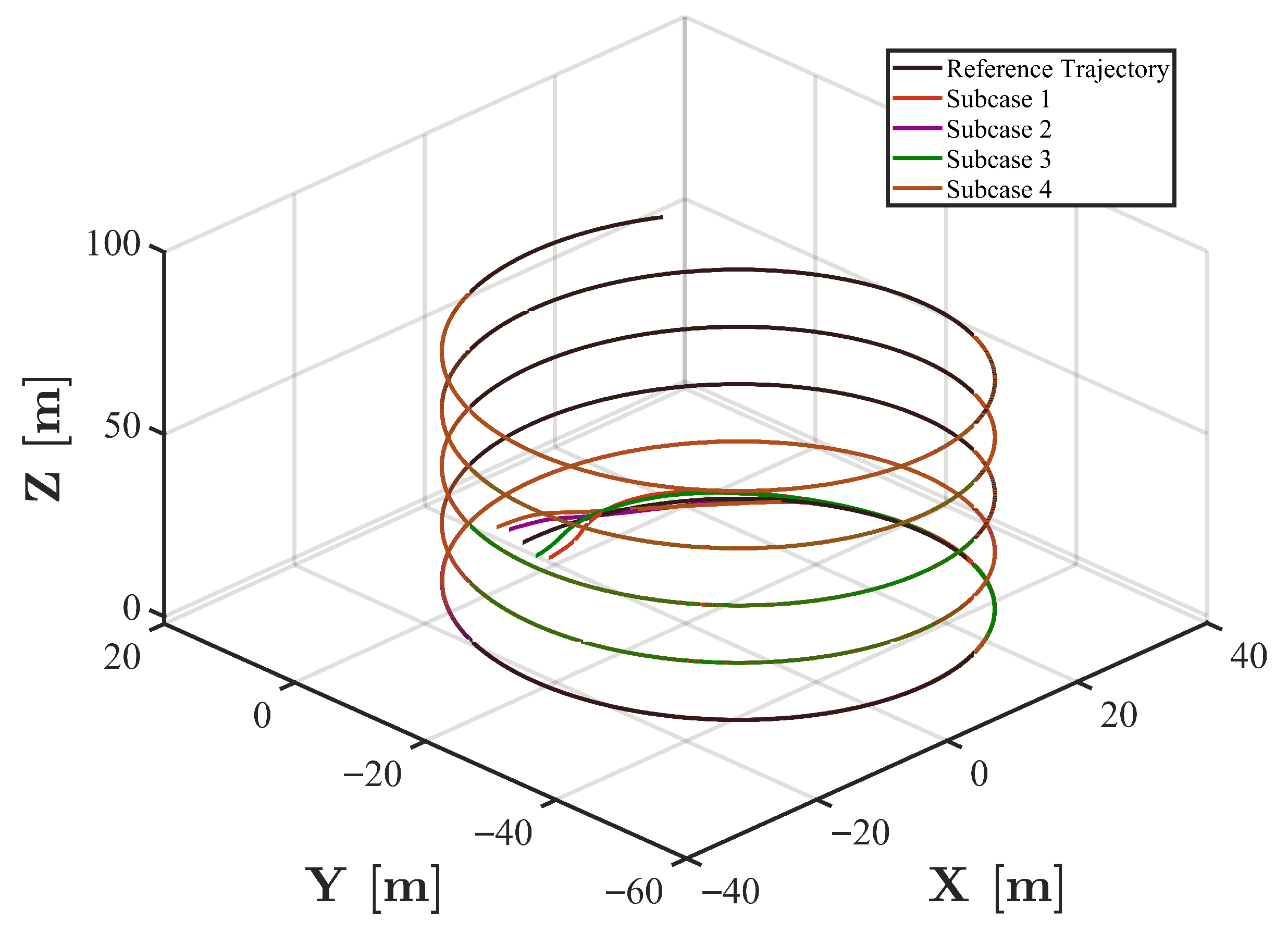
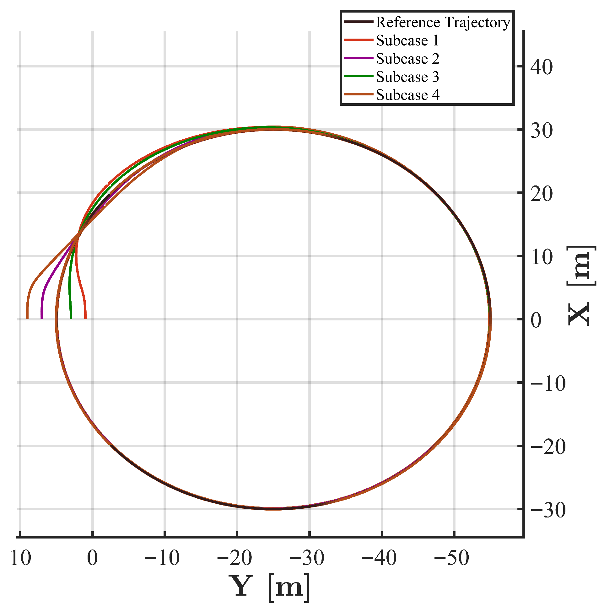
To validate the feasibility of the proposed controller, a spiral reference trajectory was considered in Scenario 1, which can be described as $x_d=30sin\left(0.04t\right)$m, $y_d=30cos\left(0.04t\right)-25$m, and $z_d=0.1t$m. To assess the adaptivity and robustness of the proposed method, four subcases with different initial positions were examined, each subjected to the same sinusoidal-type disturbances. The initial conditions for the four subcases were set as follows: (1) Subcase 1: ${[x_0,y_0,z_0,{\varphi }_0,{\theta }_0,{\psi }_0]}^T$ = ${[0 \mathrm{m},1 \mathrm{m},-1 \mathrm{m},0,0,0]}^T$; (2) Subcase 2: ${[x_0,y_0,z_0,{\varphi }_0,{\theta }_0,{\psi }_0]}^T$ = ${[0 \mathrm{m},7 \mathrm{m},2 \mathrm{m},0,0,0]}^T$; (3) Subcase 3: ${[x_0,y_0,z_0,{\varphi }_0,{\theta }_0,{\psi }_0]}^T$ = ${[0 \mathrm{m},3 \mathrm{m},-2 \mathrm{m},0,0,0]}^T$; and (4) Subcase 4: ${[x_0,y_0,z_0,{\varphi }_0,{\theta }_0,{\psi }_0]}^T$ = ${[0 \mathrm{m},9 \mathrm{m},1 \mathrm{m},0,0,0]}^T$. To mimic realistic and complex underwater conditions, the following time-varying ocean current disturbances were introduced into the AUV dynamics:

$$\left\{\begin{array}{c}{\mathrm{D}}_u=2(1.5sin\left(0.3\mathrm{t}\right)+0.6)N\hfill \\ {\mathrm{D}}_v=2(1.5sin\left(0.2\mathrm{t}\right)+0.6)N\hfill \\ {\mathrm{D}}_w=2(1.5sin\left(0.1\mathrm{t}\right)+0.6)N\hfill \\ {\mathrm{D}}_p=2(1.2sin\left(0.2\mathrm{t}\right)+0.6)Nm\hfill \\ {\mathrm{D}}_q=2(1.2sin\left(0.2\mathrm{t}\right)+0.6)Nm\hfill \\ {\mathrm{D}}_r=2(1.2sin\left(0.2\mathrm{t}\right)+0.6)Nm\hfill \end{array}\right.$$

(57)

Figure 3 and Figure 4 illustrate the 3D tracking performance and the corresponding X–Y plane projection for the four subcases under Scenario 1. In both figures, all colored trajectories, representing the four subcases, consistently converge to and follow the black reference spiral path. This uniform convergence behavior visually confirms that the controller effectively guides the AUV to the intended trajectory regardless of its initial position, demonstrating its strong adaptability and reliable performance under the given time-varying disturbances.

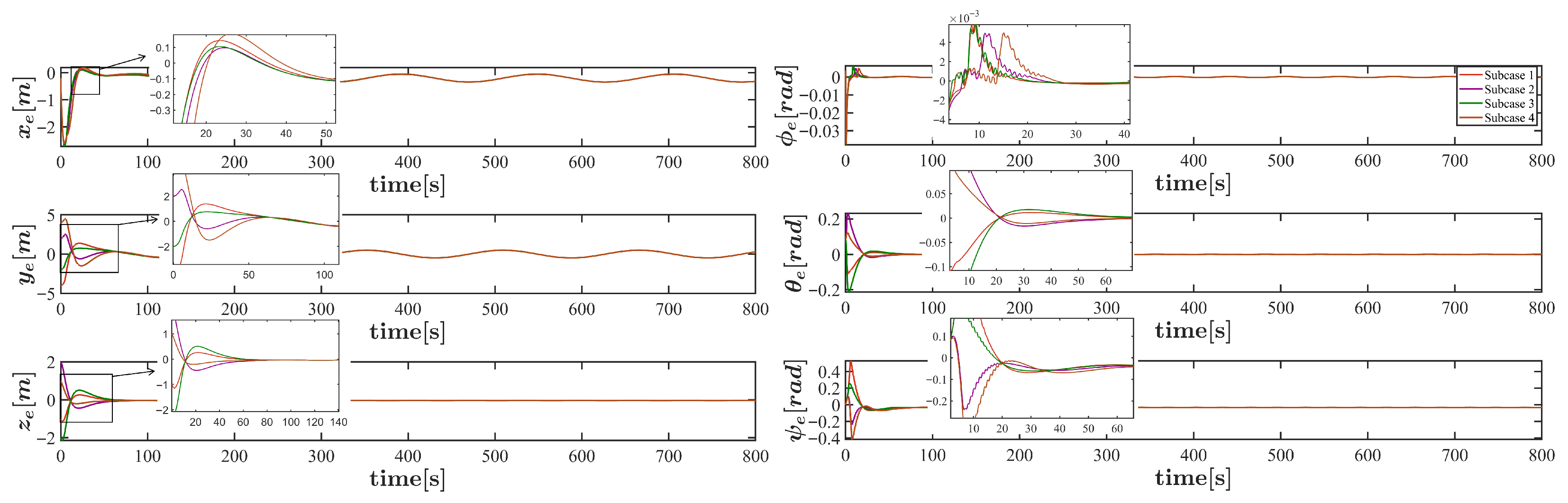
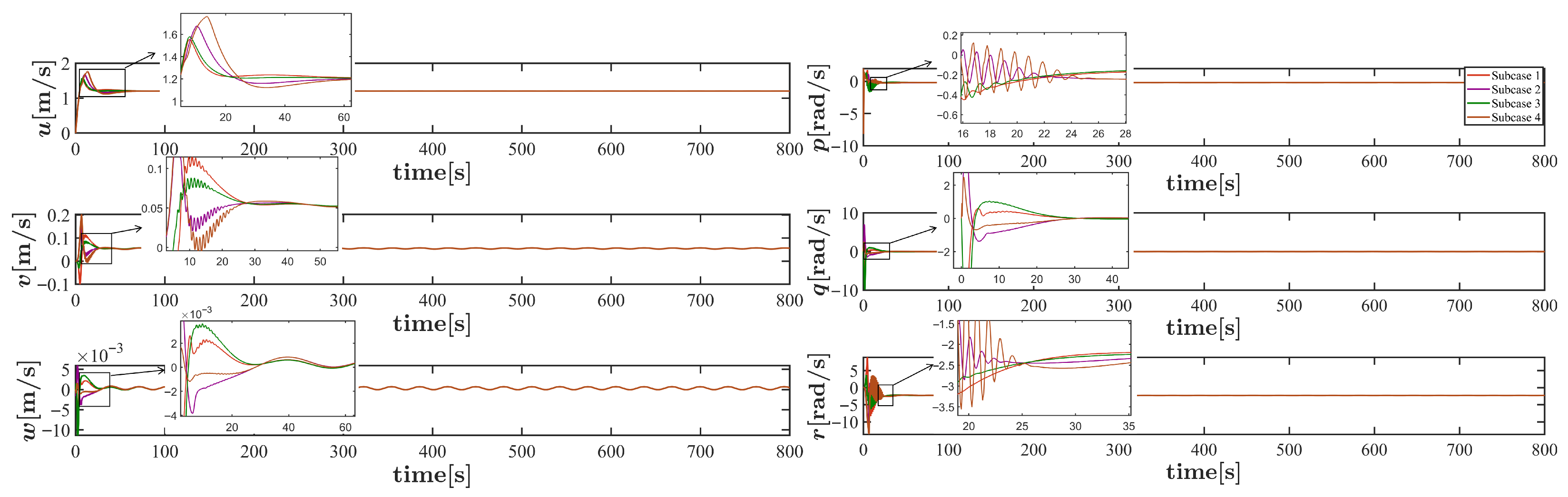
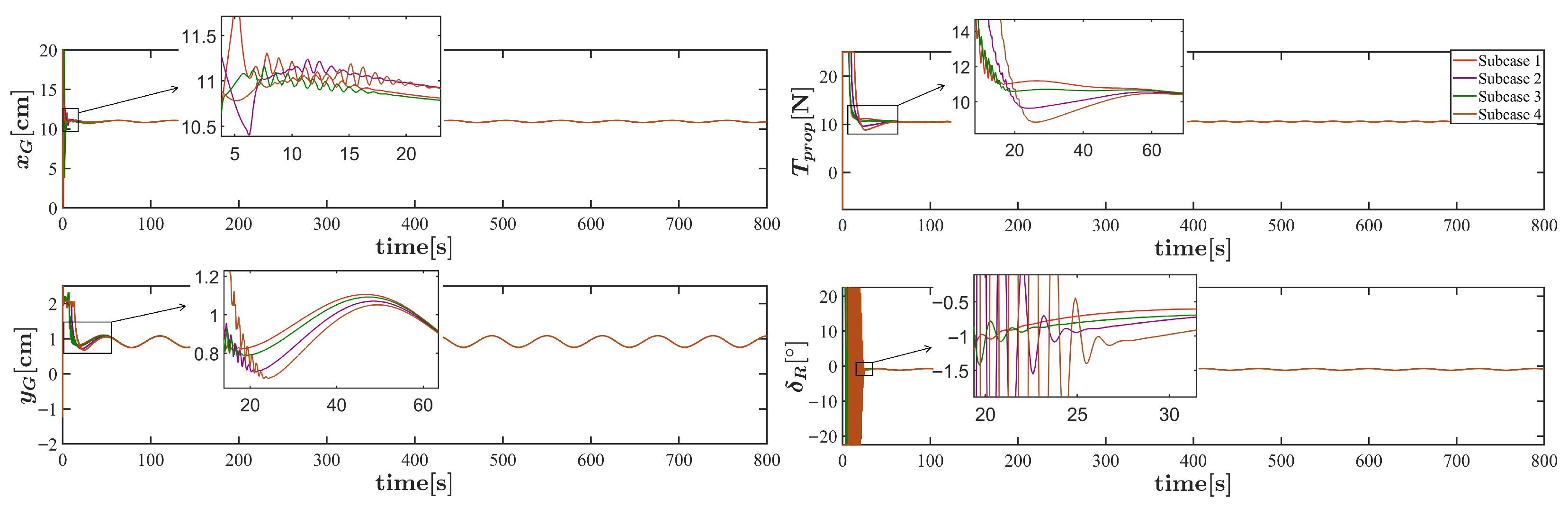
Figure 5 and Figure 6 depict the position tracking errors ${[x_e,y_e,z_e,{\varphi }_e,{\theta }_e,{\psi }_e]}^T$ and the velocity tracking results ${[u,v,w,p,q,r]}^T$ of AUV2000 under different initial conditions. The results show that both sets of result can converge consistently over time. Even under unfavorable initial conditions, the proposed controller represents only brief and small-amplitude transient oscillations during the initial phase, which is a normal characteristic of dynamic response. The subsequent steady-state errors remain within a small and stable range, confirming the correctness and convergence of the proposed scheme. Figure 7 further shows that the control inputs remain smooth and stable under all tested initial conditions, with only slight transient oscillations occurring at the beginning. Collectively, these results verify that the proposed AFtFoNTSMC strategy enables stable and effective 3D trajectory tracking for the AUV under varying initial conditions.

4.2. Scenario 2 Trajectory Tracking

This section describes the evaluation and comparison of with three widely used sliding mode control schemes, thereby highlighting the superior performance and distinctive advantages of the proposed method. In Scenario 2, a sinusoidal reference trajectory was considered, which can be depicted as $x_d=100sin\left(0.01t\right)$m, $y_d=100cos\left(0.01t\right)-95$m, and $z_d=0.1t$m. The initial conditions for the proposed AFtFoNTSMC strategy and other three comparative methods were set as follows: ${[x,y,z,\phi ,\theta ,\psi ]}^T={[0 \mathrm{m},0 \mathrm{m},-2 \mathrm{m},0,0,0]}^T$ and ${[u,v,w,p,q,r]}^T={[0,0,0,0,0,0]}^T$. Furthermore, more realistic ocean environmental disturbances, comprising sine/cosine functions and random signals, were taken into account as follows:

$$\left\{\begin{array}{c}{\mathrm{D}}_u=2.8(0.3sin\left(0.2\mathrm{t}\right)+0.4cos(0.2\mathrm{t}+1)+rand(·))N\hfill \\ {\mathrm{D}}_v=2.8(0.3sin\left(0.2\mathrm{t}\right)+0.4cos(0.2\mathrm{t}+1)+rand(·))N\hfill \\ {\mathrm{D}}_w=2.8(0.3sin\left(0.2\mathrm{t}\right)+0.4cos(0.2\mathrm{t}+1)+rand(·))N\hfill \\ {\mathrm{D}}_p=2.8(0.2sin\left(0.1\mathrm{t}\right)+0.2cos(0.2\mathrm{t}+1)+rand(·))Nm\hfill \\ {\mathrm{D}}_q=2.8(0.2sin\left(0.1\mathrm{t}\right)+0.2cos(0.2\mathrm{t}+1)+rand(·))Nm\hfill \\ {\mathrm{D}}_r=2.8(0.2sin\left(0.1\mathrm{t}\right)+0.2cos(0.2\mathrm{t}+1)+rand(·))Nm\hfill \end{array}\right.$$

(58)

where $rand(·)$ represents uniformly distributed random signals with an amplitude range of two.

These three methods considered for comparative analysis in this simulation are described as follows.

Method 1: a nonsingular fixed-time sliding mode surface ([26]) is integrated into the AUV system, and the corresponding controller is designed accordingly.

$$\left\{\begin{array}{c}{\mathit{S}}_{\mathbf{1}}=\tilde{\mathit{e}}\left(t\right)+{\mathit{l}}_{\mathbf{4}}{\int }_0^t{sig}^{2z_1-1}\mathit{e}\left(\tau \right)d\tau +{\mathit{l}}_{\mathbf{5}}{\int }_0^t{sig}^{2z_2-1}\mathit{e}\left(\tau \right)d\tau +{\mathit{l}}_{\mathbf{6}}{\int }_0^t\mathit{e}\left(\tau \right)d\tau \hfill \\ \begin{array}{cc}\hfill {\mathsf{\tau }}_{\mathbf{1}}=& \widehat{\mathit{M}}{\dot{\mathit{v}}}_{\mathbf{c}}+\widehat{\mathit{C}}\left(\mathit{v}\right)\mathit{v}+\widehat{\mathit{D}}\left(\mathit{v}\right)\mathit{v}+\widehat{\mathit{g}}\left(\mathsf{\eta }\right)-{\mathit{l}}_{\mathbf{4}}{sig}^{2z_1-1}\mathit{e}\left(t\right)\hfill \\ \hfill & -{\mathit{l}}_{\mathbf{5}}{sig}^{2z_2-1}\mathit{e}\left(t\right)-{\mathit{l}}_{\mathbf{5}}\mathit{e}\left(t\right)-{ϵ}_{s3}sign\left({\mathit{S}}_{\mathbf{3}}\right)-l_{s3}{\mathit{S}}_{\mathbf{3}}\hfill \end{array}\hfill \end{array}\right.$$

(59)

where ${\mathit{l}}_{\mathbf{4}}=diag(k_{41},\dots ,k_{4n})$, ${\mathit{l}}_{\mathbf{5}}=diag(k_{51},\dots ,k_{5n})$ and ${\mathit{l}}_{\mathbf{6}}=diag(k_{61},\dots ,k_{6n})$ satisfy that $l_{4i}>0$, $l_{5i}>0$, $l_{6i}>{\displaystyle \frac{1}{2}}(i=1,\dots ,n)$ and $0<z_1<{\displaystyle \frac{1}{2}}$ and $z_2>1$.

Method 2: a finite-time integral SMC and the controller developed in [13] are employed to achieve finite-time trajectory tracking for the AUV.

$$\left\{\begin{array}{c}{\mathit{S}}_2={\int }_0^t\tilde{\mathit{e}}\left(\tau \right)d\tau +{\mathit{l}}_2{\left({\int }_0^t\tilde{\mathit{e}}\left(\tau \right)d\tau \right)}^{{\gamma }_1}+{\mathit{l}}_3\tilde{\mathit{e}}{\left(t\right)}^{q_1}\hfill \\ \begin{array}{cc}\hfill {\mathsf{\tau }}_2& =\widehat{\mathit{M}}{\dot{\mathit{v}}}_c+\widehat{\mathit{C}}\left(\mathit{v}\right)\mathit{v}+\widehat{\mathit{D}}\left(\mathit{v}\right)\mathit{v}+\widehat{\mathit{g}}\left(\mathsf{\eta }\right)-{\displaystyle \frac{\widehat{\mathit{M}}{\mathit{l}}_3^{-1}}{q_1}}\tilde{\mathit{e}}{\left(t\right)}^{2-q_1}\hfill \\ \hfill & -{\displaystyle \frac{{\gamma }_1}{q_1}}\widehat{\mathit{M}}{\mathit{l}}_3^{-1}{\mathit{l}}_{2}diag\left({\left({\int }_0^t\tilde{\mathit{e}}\left(\tau \right)d\tau \right)}^{{\gamma }_1-1}\right)\tilde{\mathit{e}}{\left(t\right)}^{2-q_1}-{ϵ}_{s2}sign\left({\mathit{S}}_2\right)-l_{s2}{\mathit{S}}_2\hfill \end{array}\hfill \end{array}\right.$$

(60)

where ${\mathit{l}}_{\mathbf{2}}=diag(k_{21},\dots ,k_{2n})$ and ${\mathit{l}}_{\mathbf{3}}=diag(k_{31},\dots ,k_{3n})$ are all positive control parameters that need to be adjusted, and ${\gamma }_1$, $q_1>0$ satisfies $1<q_1<2$ and ${\gamma }_1>q_1$.

Method 3: a robust integral sliding mode surface introduced in [5] and its associated controller are adopted for comparative analysis.

$$\left\{\begin{array}{c}{\mathit{S}}_{\mathbf{3}}=\tilde{\mathit{e}}\left(t\right)+{\mathit{l}}_{\mathbf{1}}{\int }_0^t\tilde{\mathit{e}}\left(\tau \right)d\tau \hfill \\ {\mathsf{\tau }}_{\mathbf{3}}=\widehat{\mathit{M}}{\dot{\mathit{v}}}_{\mathbf{c}}+\widehat{\mathit{C}}\left(\mathit{v}\right)\mathit{v}+\widehat{\mathit{D}}\left(\mathit{v}\right)\mathit{v}+\widehat{\mathit{g}}\left(\mathsf{\eta }\right)-{\mathit{l}}_{\mathbf{1}}\tilde{\mathit{e}}\left(t\right)-{ϵ}_{s1}sign\left({\mathit{S}}_{\mathbf{1}}\right)-l_{s1}{\mathit{S}}_{\mathbf{1}}\hfill \end{array}\right.$$

(61)

where ${\mathit{l}}_{\mathbf{1}}=diag(l_{11},\dots ,l_{1n}])$ and $l_{1i}$ denotes the positive control parameter.

Compared with Method 1, the proposed FoNTSM exhibited superior performance in both stabilization speed and chattering suppression over the existing fixed-time sliding surface. Similarly, when compared with Method 2 and Method 3, the AFtFoNTSMC strategy, based on fixed-time control theory, demonstrated superior transient and steady-state performance over existing asymptotically stable and finite-time stable approaches. To ensure the effectiveness and fairness of the comparative methods, we tried to maintain consistent parameter settings for corresponding terms across all three methods. Specifically, the power reaching law parameters for all three comparative methods were configured uniformly as ${ϵ}_{s1}={ϵ}_{s2}={ϵ}_{s3}=1$ and $l_{s1}=l_{s2}=l_{s3}=1.2$, and the other parameters are detailed in

Table 2. Parameter settings for the three methods compared.

	Parameter
Method 1	$\begin{array}{c}{\mathit{l}}_{\mathbf{4}}=diag(0.8,0.8,0.8,1,1,1), {\mathit{l}}_{\mathbf{5}}=diag(1.2,1.2,1.2,0.9,0.9,1.2)\hfill \\ {\mathit{l}}_{\mathbf{6}}=diag(0.6,0.6,0.6,0.5,0.5,0.5), z_1={\displaystyle \frac{7}{11}} ,z_2={\displaystyle \frac{9}{5}}\hfill \end{array}$
Method 2	$\begin{array}{c}{\mathit{l}}_{\mathbf{2}}=diag(1,1,1,1,1,1), {\mathit{l}}_{\mathbf{3}}=diag(1.2,1.2,1,0.8,1.2,1.8), {\gamma }_1=3.8, q_1=1.7\hfill \end{array}$
Method 3	$\begin{array}{c}{\mathit{l}}_{\mathbf{1}}=diag(0.5,0.5,0.5,1,1,1)\hfill \end{array}$

.

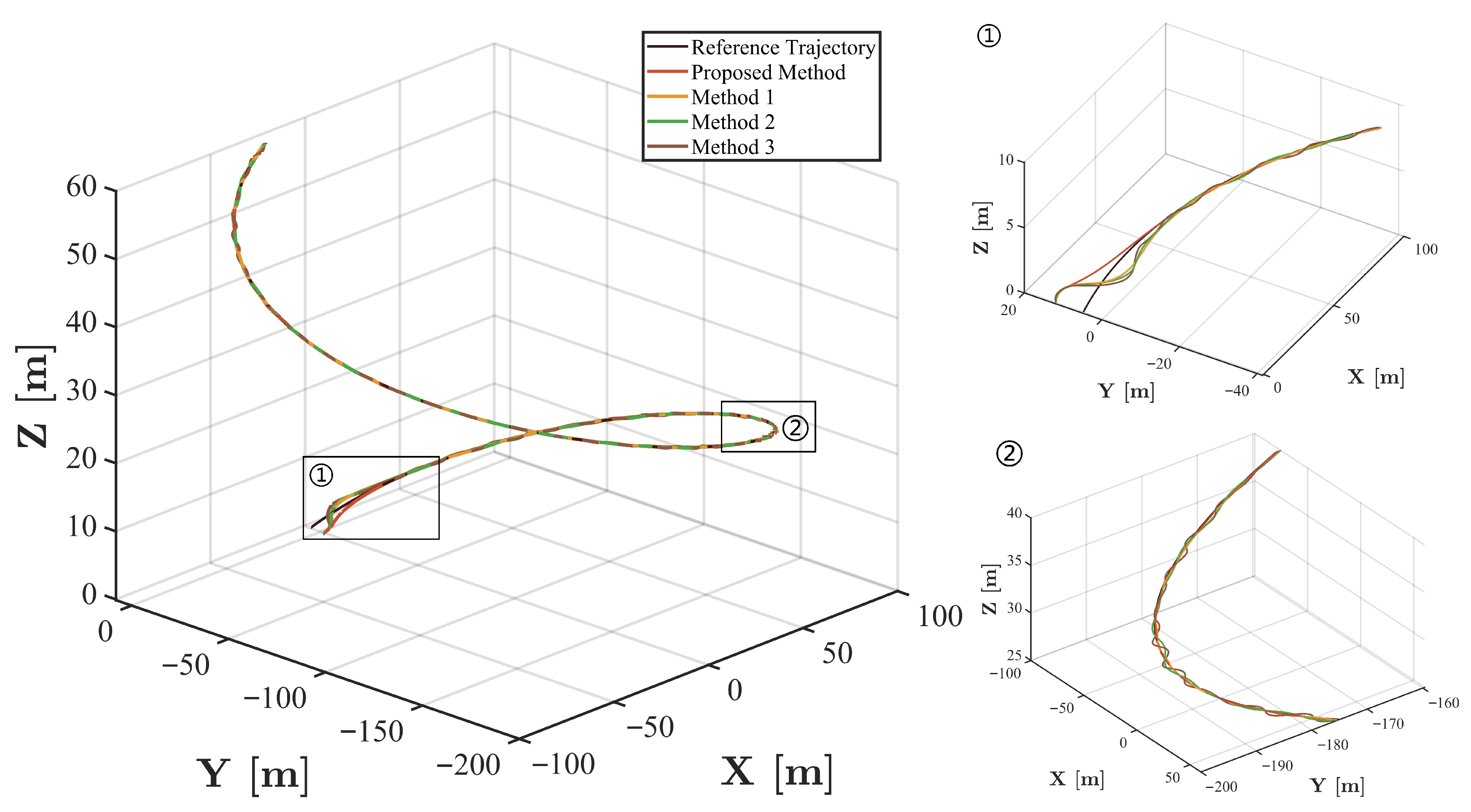
Figure 8 shows a 3D visualization of AUV’s trajectory tracking performance in the four different control methods. The two close-up views clearly illustrate the goodness of the proposed strategy: (1) In the initial stage (first close-up view), the proposed method converges the fastest, with almost no oscillation. (2) During the mid-phase (second close-up view), it maintains the most stable dynamic behavior, following the reference trajectory closely with minimal overshoot. In contrast, the other three methods exhibit noticeable oscillation, deviation, or slower convergence in one or both of these phases.

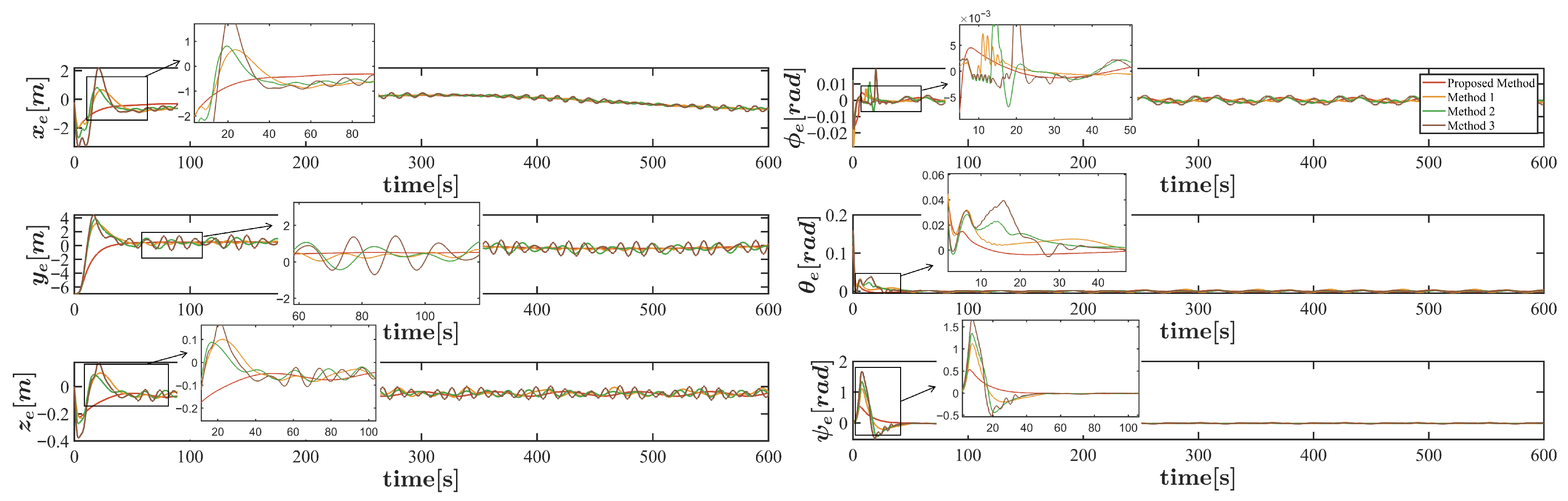
Figure 9 compares the position tracking errors between the proposed AFtFoNTSMC strategy and three benchmark methods. Across all six degrees of freedom, the proposed method consistently achieves superior performance. Specifically, in the $x_e$ subplot, it converges faster and stabilizes within 30 s, whereas the other methods require at least 50 s. In the $y_e$ subplot, the proposed method exhibits minimal oscillation in the steady state. This advantage can be attributed to the newly designed adaptive algorithm, which effectively enhances robustness against external disturbances. In the other subplots, the proposed method also shows the least oscillation and fastest convergence rate during the initial transient phase.

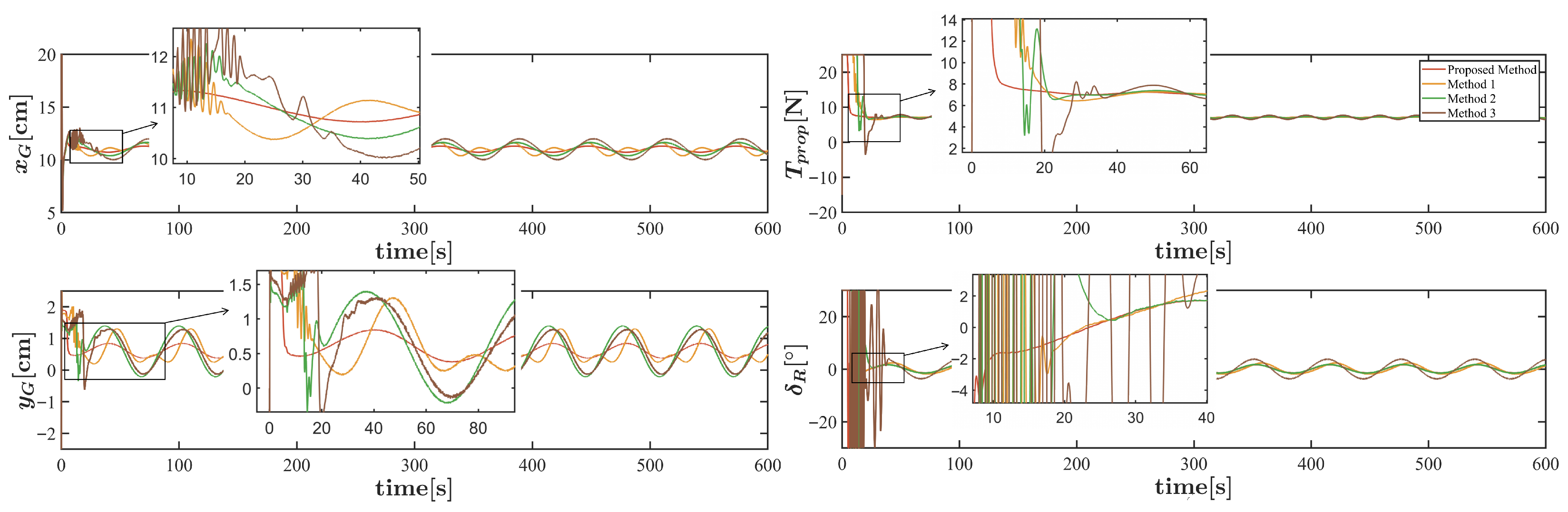
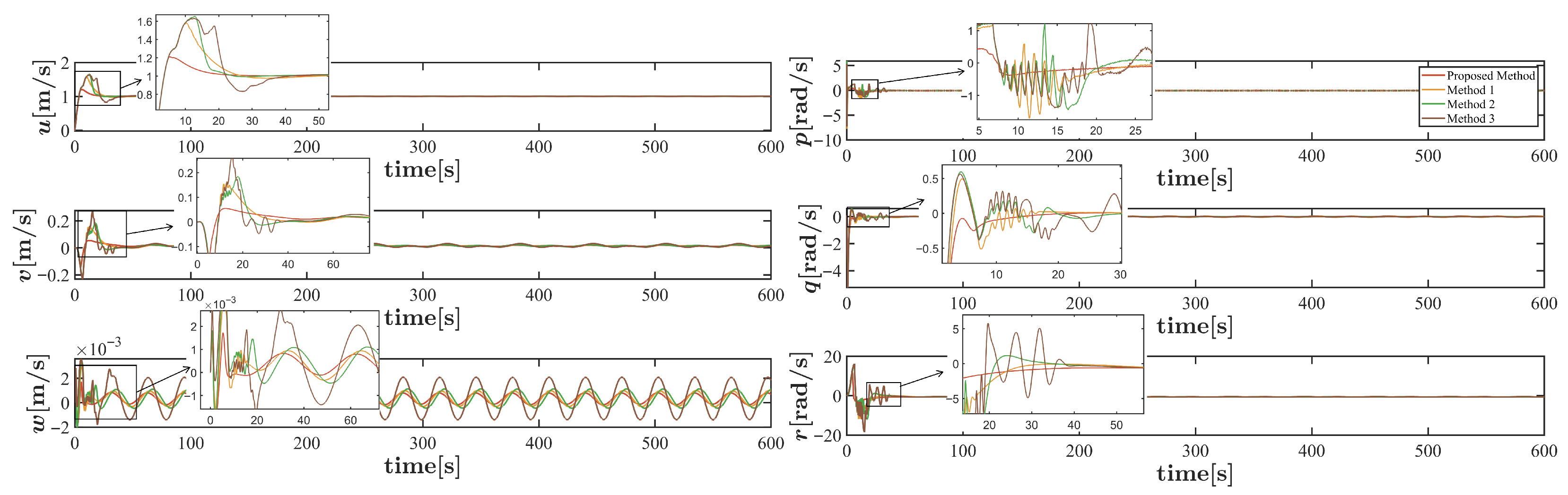
Figure 10 compares the velocity tracking results of AUV2000. The proposed strategy shows faster convergence, lower oscillation, and minimal overshoot across all degrees of freedom, demonstrating its superior accuracy, robustness, and stability over the benchmarks. Figure 11 presents the four control inputs generated by the three control strategies. Although all three methods display periodic vibrations during the steady state due to external disturbances, the proposed AFtFoNTSMC stands out with fastest convergence and lowest vibration amplitudes. This vibration reduction in control inputs contributes to lower energy consumption and extended service life of facilities, thereby further demonstrating the reliability of AFtFoNTSMC in practical AUV applications.

To quantitatively evaluate the performance of the proposed AFtFoNTSMC strategy, two performance evaluation indices, the mean absolute value of the tracking error ($MAE$) and the mean of the square value of the tracking error ($MSE$) were employed. These metrics are formulated as follows:

$$\left\{\begin{array}{cc}\hfill & \mathrm{MAE}={\displaystyle \frac{1}{n}}\sum _{i=1}^n\left|{\tilde{e}}_i-{\widehat{\tilde{e}}}_i\right|\hfill \\ \hfill & \mathrm{MSE}={\displaystyle \frac{1}{n}}\sum _{i=1}^n{\left({\tilde{e}}_i-{\widehat{\tilde{e}}}_i\right)}^2\hfill \end{array}\right.$$

(62)

Table 3. Quantitative analysis of different controllers.

Performance Index ($\ast {10}^{-2}$)	Proposed Method	Method 1	Method 2	Method 3
$MAE\left(x_e\right)$	27.74	34.10	36.48	39.52
$MAE\left(y_e\right)$	44.13	52.58	62.03	70.92
$MAE\left(z_e\right)$	4.27	5.43	5.37	5.83
$MAE\left(ph{i}_e\right)$	0.01	0.07	0.04	0.15
$MAE\left(thet{a}_e\right)$	0.12	0.32	0.19	0.25
$MAE\left(ps{i}_e\right)$	2.08	3.18	3.73	4.08
$TotalMAE$	13.06	15.94	17.97	20.13
$MSE\left(x_e\right)$	11.88	17.33	20.08	34.93
$MSE\left(y_e\right)$	82.26	97.72	113.69	124.98
$MSE\left(z_e\right)$	0.21	0.36	0.35	0.51
$MSE\left(ph{i}_e\right)$	0	0	0	0
$MSE\left(thet{a}_e\right)$	0	0.01	0	0.01
$MSE\left(ps{i}_e\right)$	0.34	1.22	0.93	2.96
$TotalMSE$	15.78	19.44	22.51	27.23

provides a quantitative comparison of the four control strategies. These results shows that the proposed method has the best performances in all measured error metrics. Specifically, the total MAE of the proposed method is 13.06, corresponding to reductions of approximately $18\%$, $27\%$, and $35\%$ compared to Method 1, Method 2, and Method 3, respectively. Similarly, for the total MSE, the proposed controller attains a value of 15.78, which is about $19\%$, $30\%$, and $42\%$ lower than those of Method 1, Method 2, and Method 3, respectively. The results further verify the high accuracy of the proposed method in guiding the AUV toward the desired reference trajectory.

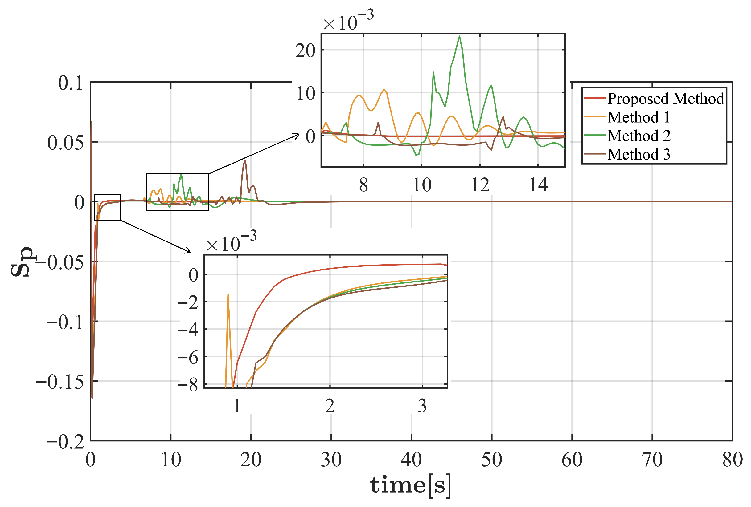
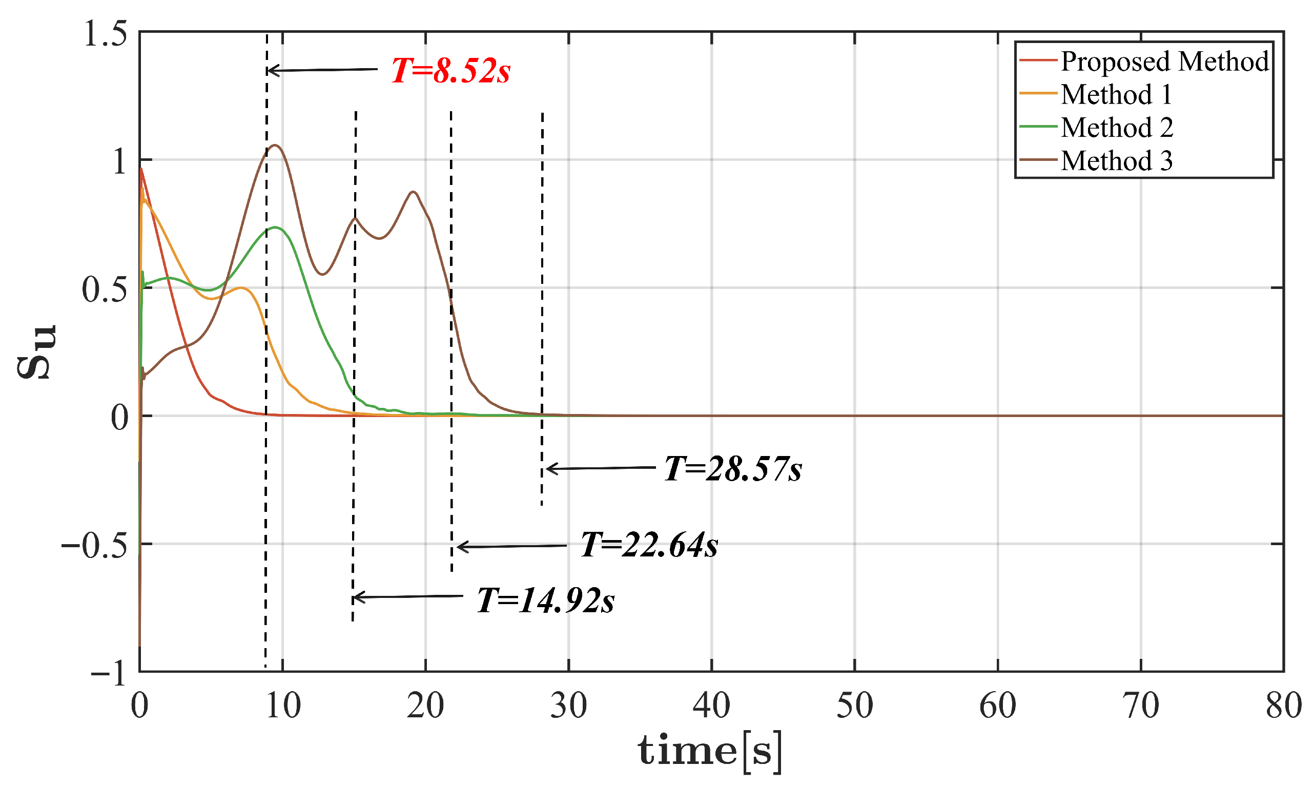
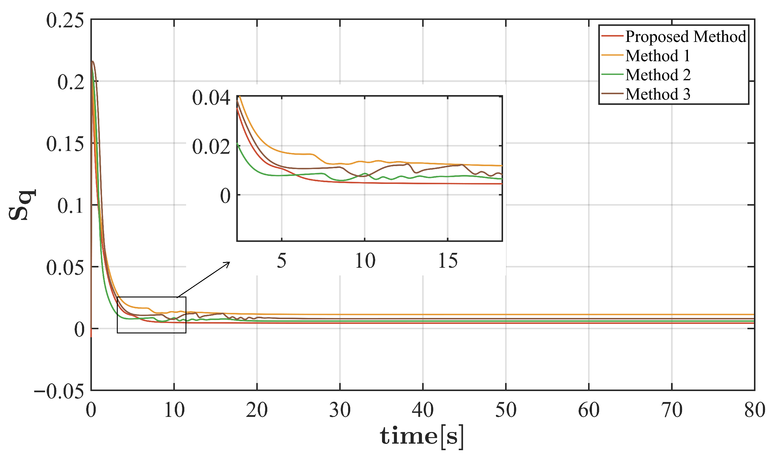
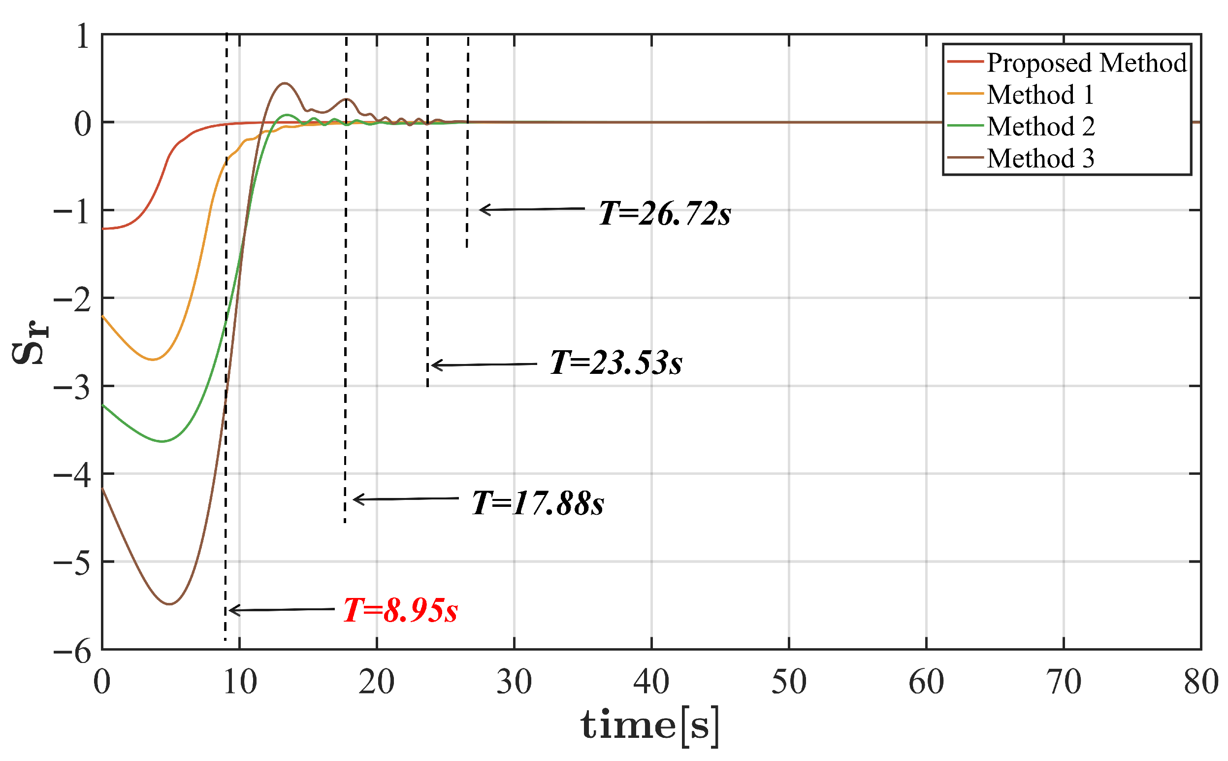
Since AUV2000 is an underactuated AUV, the degree of freedom in its control input ${\tau }_v={[T_{prop},0,0,y_G,x_G,{\delta }_R]}^T$ is limited to four. To evaluate the convergence performance of the proposed method, the corresponding four sliding mode surfaces $S_u$,$S_p$,$S_q$ and $S_r$ were compared and are displayed in Figure 12, Figure 13, Figure 14 and Figure 15. As shown in Figure 12, the convergence time of $S_u$ achieved by the proposed method is only 14.92 s, which represents a reduction of $43\%$, $62\%$ and $70\%$ compared to that of Method 1, Method 2, and Method 3, respectively. Likewise, Figure 15 indicates that the $S_r$ sliding surface under the proposed scheme converges in 8.95 s, which is notably earlier than the 17.88 s, 23.53 s, and 26.72 s required by Methods 1, 2, and 3, respectively. Meanwhile, Figure 13 and Figure 14 demonstrate that the proposed AFtFoNTSMC not only converges faster but also exhibits significantly lower oscillations than do the other benchmark methods. Taken together, these quantitative results validate the superiority of the proposed method for steady-state performance and convergence speed.

The proposed AFtFoNTSMC strategy demonstrates superior performance over conventional methods. Firstly, as proven in Theorem 2, the control law, derived from Lyapunov stability analysis, guarantees fixed-time convergence of tracking errors with the convergence time bounded independently of initial conditions, thereby ensuring rapid and predictable stabilization. The explicit upper bound formula (Equation (55)) for the convergence time provides a clear theoretical foundation for the fast and consistent convergence performance observed in the simulation case studies. Secondly, the designed FoNTSM surface, utilizing FO calculus, significantly reduces chattering, which is a key theoretical advantage that was directly validated in the simulation results (e.g., Figure 12, Figure 13, Figure 14 and Figure 15) by the smoothness of the control inputs. It achieves fast convergence with an explicitly bounded maximum settling time, thus improving navigation predictability. Crucially, the novel FO adaptive law (Equation (43)) effectively compensates for external disturbances without requiring prior knowledge of their bounds, thereby ensuring strong robustness. This theoretical design is directly linked to the simulation’s realistic disturbance rejection, as demonstrated in Scenario 1 (Equation (57)) and the more complex, random-disturbance environment of Scenario 2 (Equation (58)). The above simulation results confirm that the proposed strategy outperforms three widely used benchmark methods in trajectory tracking performance, quantitatively validating the theoretical claims (e.g., Table 3). In conclusion, the AFtFoNTSMC strategy with a dual-loop control architecture offers high control precision and robust performance for 3D sinusoidal trajectory tracking of AUVs, as evidenced by the close link between its theoretical fixed-time guarantees and its practical simulation validation.

5. Conclusions

In this paper, a novel global AFtFoNTSMC control strategy is proposed for an underactuated AUV in the presence of unknown lumped disturbances. Through the integration of fixed-time control theorem, a new FoNTSM manifold was developed, effectively reducing chattering and eliminating the singularity problem commonly encountered in conventional TSMC design. To mitigate the adverse effects of unknown lumped disturbances, a fractional-order adaptive law was designed, significantly enhancing the system’s robustness. The proposed AFtFoNTSMC controller, based on a fractional-order reaching law, was rigorously proven to stabilize under Lyapunov condition, ensuring that the AUV’s tracking errors can achieve fixed-time convergence with high accuracy. Notably, the convergence time is bounded, and its upper bound is independent of the initial system state, providing predictable performance in practical applications. The extensive simulations under two distinct scenarios, which were spiral and sinusoidal reference trajectories under various ocean disturbances, have intuitively and quantitatively verified the effectiveness, robustness, and feasibility of the proposed control strategy.

However, it should be acknowledged that the proposed method exhibits certain limitations. First, the controller’s performance relies on the appropriate selection of fractional-order parameters and adaptive gains, which may require considerable tuning effort in the absence of systematic guidelines. Second, although the adaptive law enhances robustness, its effectiveness under extreme disturbance conditions, such as abruptly time-varying or non-smooth disturbances, remains to be fully investigated. Future work will focus on integrating reinforcement learning techniques into the AFtFoNTSMC framework to further enhance adaptability and control performance, as well as conducting real-world experiments to provide additional validation of its practical applicability.

References

1. Nicholson, J.; Healey, A. The present state of autonomous underwater vehicle (AUV) applications and technologies. Mar. Technol. Soc. J. 2008, 42, 44–51. [Google Scholar] [CrossRef]
2. Hu, Y.; Song, Z.; Zhang, H. Adaptive sliding mode control with pre-specified performance settings for AUV’s trajectory tracking. Ocean. Eng. 2023, 287, 115882. [Google Scholar] [CrossRef]
3. Li, D.; Du, L. Auv trajectory tracking models and control strategies: A review. J. Mar. Sci. Eng. 2021, 9, 1020. [Google Scholar] [CrossRef]
4. Elmokadem, T.; Zribi, M.; Youcef-Toumi, K. Trajectory tracking sliding mode control of underactuated AUVs. Nonlin. Dyn. 2016, 84, 1079–1091. [Google Scholar] [CrossRef]
5. Yan, Z.; Wang, M.; Xu, J. Robust adaptive sliding mode control of underactuated autonomous underwater vehicles with uncertainCuong dynamics. Ocean. Eng. 2019, 173, 802–809. [Google Scholar] [CrossRef]
6. Li, J.; Guo, H.; Zhang, H.; Yan, Z. Double-loop structure integral sliding mode control for UUV trajectory tracking. IEEE Access 2019, 7, 101620–101632. [Google Scholar] [CrossRef]
7. Guo, Y.; Qin, H.; Xu, B.; Han, Y.; Fan, Q.Y.; Zhang, P. Composite learning adaptive sliding mode control for AUV target tracking. Neurocomputing 2019, 351, 180–186. [Google Scholar] [CrossRef]
8. Yan, Y.; Yu, S. Sliding mode tracking control of autonomous underwater vehicles with the effect of quantization. Ocean. Eng. 2018, 151, 322–328. [Google Scholar] [CrossRef]
9. Tang, Y. Terminal sliding mode control for rigid robots. Automatica 1998, 34, 51–56. [Google Scholar] [CrossRef]
10. Wu, Z.; Peng, H.; Hu, B.; Feng, X. Trajectory tracking of a novel underactuated AUV via nonsingular integral terminal sliding mode control. IEEE Access 2021, 9, 103407–103418. [Google Scholar] [CrossRef]
11. Ramezani-al, M.R.; Tavanaei Sereshki, Z. A novel adaptive sliding mode controller design for tracking problem of an AUV in the horizontal plane. Int. J. Dyn. Control 2019, 7, 679–689. [Google Scholar] [CrossRef]
12. Li, B.; Gao, X.; Huang, H.; Yang, H. Improved adaptive twisting sliding mode control for trajectory tracking of an AUV subject to uncertainties. Ocean. Eng. 2024, 297, 116204. [Google Scholar] [CrossRef]
13. Qiao, L.; Zhang, W. Trajectory tracking control of AUVs via adaptive fast nonsingular integral terminal sliding mode control. IEEE Trans. Ind. Inform. 2019, 16, 1248–1258. [Google Scholar] [CrossRef]
14. Su, B.; Wang, H.; Li, N. Event-triggered integral sliding mode fixed time control for trajectory tracking of autonomous underwater vehicle. Trans. Inst. Meas. Control 2021, 43, 3483–3496. [Google Scholar] [CrossRef]
15. Long, H.; Zhang, P.; Guo, T.; Zhao, J. Saturated Adaptive Fuzzy Fixed-Time Nonsingular Integral Terminal Sliding-Mode Control of AUVs. IEEE Trans. Cybern. 2025, 55, 1634–1647. [Google Scholar] [CrossRef]
16. An, S.; Wang, L.; He, Y. Robust fixed-time tracking control for underactuated AUVs based on fixed-time disturbance observer. Ocean. Eng. 2022, 266, 112567. [Google Scholar] [CrossRef]
17. Zhu, Z.; Duan, Z.; Qin, H.; Xue, Y. Adaptive neural network fixed-time sliding mode control for trajectory tracking of underwater vehicle. Ocean. Eng. 2023, 287, 115864. [Google Scholar] [CrossRef]
18. Zhu, Z.; To, S.; Li, Y.; Zhu, W.L.; Bian, L. External force estimation of a piezo-actuated compliant mechanism based on a fractional order hysteresis model. Mech. Syst. Signal Process. 2018, 110, 296–306. [Google Scholar] [CrossRef]
19. Tuan, L.A. Fractional-order fast terminal back-stepping sliding mode control of crawler cranes. Mech. Mach. Theory 2019, 137, 297–314. [Google Scholar] [CrossRef]
20. Huang, S.; Xiong, L.; Wang, J.; Li, P.; Wang, Z.; Ma, M. Fixed-time fractional-order sliding mode controller for multimachine power systems. IEEE Trans. Power Syst. 2020, 36, 2866–2876. [Google Scholar] [CrossRef]
21. Zhao, J.; Lin, Z.; Xiao, M.; Gao, Z.; Ding, J. A novel fixed-time fractional order nonsingular terminal sliding mode control. Asian J. Control 2023, 25, 3660–3670. [Google Scholar] [CrossRef]
22. Delavari, H.; Heydarinejad, H.; Baleanu, D. Adaptive fractional-order blood glucose regulator based on high-order sliding mode observer. IET Syst. Biol. 2019, 13, 43–54. [Google Scholar] [CrossRef]
23. Gao, P.; Zhang, G.; Ouyang, H.; Mei, L. An adaptive super twisting nonlinear fractional order PID sliding mode control of permanent magnet synchronous motor speed regulation system based on extended state observer. IEEE Access 2020, 8, 53498–53510. [Google Scholar] [CrossRef]
24. Zhang, D.; Hu, J.; Cheng, J.; Wu, Z.G.; Yan, H. A novel disturbance observer based fixed-time sliding mode control for robotic manipulators with global fast convergence. IEEE/CAA J. Autom. Sin. 2024, 11, 661–672. [Google Scholar] [CrossRef]
25. Huang, S.; Wang, J.; Huang, C.; Zhou, L.; Xiong, L.; Liu, J.; Li, P. A fixed-time fractional-order sliding mode control strategy for power quality enhancement of PMSG wind turbine. Int. J. Electr. Power Energy Syst. 2022, 134, 107354. [Google Scholar] [CrossRef]
26. Chen, Q.; Wang, L.; Sun, Y.; Xie, S.; Wang, R. Adaptive integral sliding mode MPPT control for wind turbines with fixed-time convergence. IET Renew. Power Gener. 2024, 18, 4265–4276. [Google Scholar] [CrossRef]
27. Ahmed, S.; Ghous, I.; Mumtaz, F. TDE based model-free control for rigid robotic manipulators under nonlinear friction. Sci. Iran. 2024, 31, 137–148. [Google Scholar] [CrossRef]
28. Pudlubny, I. Fractional Differential Equations; Mathematics in Science and Engineering; Academic Press: New York, NY, USA, 1999. [Google Scholar]
29. Lei, C.; Lan, Y.; Sun, Y.; Xu, Z.; Shi, X. Fixed-time convergence of second-order nonlinear systems based on nonsingular fractional sliding mode. Trans. Inst. Meas. Control 2024, 46, 1885–1891. [Google Scholar] [CrossRef]
30. Cuong, H.M.; Van Thai, N.; Van Trieu, P.; Dong, H.Q.; Nam, T.T.; Viet, T.X.; Nho, L.C.; Tuan, L.A. Nonsingular fractional-order integral fast-terminal sliding mode control for underactuated shipboard cranes. J. Frankl. Inst. 2022, 359, 6587–6606. [Google Scholar] [CrossRef]
31. Tran, H.N.; Pham, T.N.N.; Choi, S.H. Robust depth control of a hybrid autonomous underwater vehicle with propeller torque’s effect and model uncertainty. Ocean. Eng. 2021, 220, 108257. [Google Scholar] [CrossRef]
32. Shojaei, K.; Arefi, M.M. On the neuro-adaptive feedback linearising control of underactuated autonomous underwater vehicles in three-dimensional space. IET Control Theory Appl. 2015, 9, 1264–1273. [Google Scholar] [CrossRef]
33. Qiao, L.; Zhang, W. Double-loop integral terminal sliding mode tracking control for UUVs with adaptive dynamic compensation of uncertainties and disturbances. IEEE J. Ocean. Eng. 2018, 44, 29–53. [Google Scholar] [CrossRef]
34. Fossen, T.I. Handbook of Marine Craft Hydrodynamics and Motion Control; John Wiley & Sons: Hoboken, NJ, USA, 2011. [Google Scholar]
35. Thanh, P.N.N.; Tam, P.M.; Anh, H.P.H. A new approach for three-dimensional trajectory tracking control of underactuated AUVs with model uncertainties. Ocean. Eng. 2021, 228, 108951. [Google Scholar] [CrossRef]
36. Radac, M.B.; Precup, R.E. Data-driven MIMO model-free reference tracking control with nonlinear state-feedback and fractional order controllers. Appl. Soft Comput. 2018, 73, 992–1003. [Google Scholar] [CrossRef]
37. Radac, M.B.; Chirla, D.P. Near real-time online reinforcement learning with synchronous or asynchronous updates. Sci. Rep. 2025, 15, 17158. [Google Scholar] [CrossRef] [PubMed]
Figure 1. The body-fixed and earth-fixed coordinate systems of AUV2000.
Drones 10 00198 g001
Figure 2. Schematic of the proposed dual closed-loop AFtFoNTSMC control system for AUV trajectory tracking.
Drones 10 00198 g002
Figure 3. 3D Tracking results across different subcases under Scenario 1.
Drones 10 00198 g003
Figure 4. Two-dimensional (X–Y) plane projection of the tracking results under Scenario 1.
Drones 10 00198 g004
Figure 5. Position tracking errors: [ x e , y e , z e , ϕ e , θ e , ψ e ] T for AUV2000 across different initial states under Scenario 1.
Drones 10 00198 g005
Figure 6. Velocity tracking results: [ u , v , w , p , q , r ] T for AUV2000 across different initial states under Scenario 1.
Drones 10 00198 g006
Figure 7. Control inputs: x G , y G , T p r o p , and δ R for AUV2000 across different initial states under Scenario 1.
Drones 10 00198 g007
Figure 8. Comparison of 3D trajectory tracking results among the proposed AFtFoNTSMC method and three benchmark methods with lumped disturbances under Scenario 2.
Drones 10 00198 g008
Figure 9. Comparison of position tracking errors [ x e , y e , z e , ϕ e , θ e , ψ e ] T for AUV2000: proposed AFTO versus three benchmark methods under Scenario 2.
Drones 10 00198 g009
Figure 10. Comparison of velocity tracking results [ u , v , w , p , q , r ] T for AUV2000: proposed AFTO versus three benchmark methods under Scenario 2.
Drones 10 00198 g010
Figure 11. Comparison of control inputs x G , y G , T p r o p , and δ r for AUV2000: proposed AFtFoNTSMC versus three benchmark methods under Scenario 2.
Drones 10 00198 g011
Figure 12. Comparison of sliding mode S u between the proposed AFtFoNTSMC and three benchmark methods under Scenario 2.
Drones 10 00198 g012
Figure 13. Comparison of sliding mode S p between the proposed AFtFoNTSMC and three benchmark methods under Scenario 2.
Drones 10 00198 g013
Figure 14. Comparison of sliding mode S q between the proposed AFtFoNTSMC and three benchmark methods under Scenario 2.
Drones 10 00198 g014
Figure 15. Comparison of sliding mode S r between the Proposed AFtFoNTSMC and three benchmark methods under Scenario 2.
Drones 10 00198 g015