Second-Order L1 Schemes for Fractional Differential Equations

Abstract

Difference schemes for the numerical solution of fractional differential equations rely on discretizations of the fractional derivative. In this paper, we obtain the second-order expansion formula for the L1 approximation of the Caputo fractional derivative. Second-order approximations of the fractional derivative are constructed based on the expansion formula and parameter-dependent discretizations of the second derivative. Examples illustrating the application of these approximations to the numerical solution of ordinary and partial fractional differential equations are presented, and the convergence and order of the difference schemes are proved. Numerical experiments are also provided, confirming the theoretical predictions for the accuracy of the numerical methods.

1. Introduction

Fractional differentiation extends integer-order differentiation and integration to arbitrary orders. There is a growing interest in developing high-order numerical methods for fractional differential equations due to their wide applicability in various branches of science [1,2,3,4]. Finite difference schemes provide a powerful approach for the numerical solution of fractional differential equations and the study of their properties. The Caputo fractional derivative of order $\alpha$, where $0<\alpha <1$ is defined as

$$f^{\left(\alpha \right)}\left(x\right)=D^{\alpha }f\left(x\right)={\displaystyle \frac{1}{\Gamma (1-\alpha )}}{\int }_0^x{\displaystyle \frac{f^{\prime }\left(\xi \right)}{{(x-\xi )}^{\alpha }}}d\xi .$$

(1)

The power function $x^p$ and the functions $e^x$, $sinx$, and $cosx$ have fractional derivatives

$$D^{\alpha }{x}^p={\displaystyle \frac{\Gamma (p+1)}{\Gamma (p+1-\alpha )}}{x}^{p-\alpha },D^{\alpha }{e}^x=x^{1-\alpha }{E}_{1,2-\alpha }\left(x\right),$$

$$D^{\alpha }sinx=x^{1-\alpha }{E}_{2,2-\alpha }(-x^2),D^{\alpha }cosx=-x^{2-\alpha }{E}_{2,3-\alpha }(-x^2),$$

where $p>0$ and $E_{\alpha ,\beta }\left(x\right)$ is the Mittag-Leffler function

$$E_{\alpha ,\beta }\left(x\right)=\sum _{k=0}^{\infty }{\displaystyle \frac{x^k}{\Gamma (\alpha x+\beta )}}.$$

The lower limit of fractional differentiation may be an arbitrary number. The kernel of the fractional derivative has a singularity of order $\alpha$, and therefore a direct application of numerical integration methods to construct discretizations of the fractional derivative leads to reduced accuracy and a lower order of approximation. Consequently, constructing high-order approximations of fractional derivatives requires additional considerations.

Fractional calculus is a rapidly developing scientific field that extends and generalizes differential calculus. Other definitions of fractional derivatives and integrals include the Riemann–Liouville and Grünwald–Letnikov derivatives, introduced in the 19th century. The Riemann–Liouville derivative is the first known generalization of integer-order derivatives and is a widely used definition in fractional calculus. The three definitions of the fractional derivative are directly related and share similar properties. The main difference between fractional and integer-order derivatives lies in their nonlocal nature. Fractional derivatives strongly depend on the previous values of the function according to a power law or exhibit memory-influenced dynamics. The choice of a particular definition of the fractional derivative and its advantages depends on the problem under consideration. The Caputo fractional derivative, introduced in 1967, has the advantage that, when solving differential equations, it allows the use of initial conditions expressed in terms of integer-order derivatives, which often have direct physical meaning. In addition to the three most commonly used definitions of the fractional derivative, there exist other important definitions in the theory of fractional calculus. Among them are the fractional derivatives of Weyl, Hadamard, Marchaud, and Riesz.

Fractional differential equations generalize ordinary and partial differential equations and provide powerful tools for modeling anomalous diffusion processes and complex systems with memory and hereditary properties. Due to the complexity of fractional differential equations and the models they describe, numerical methods are the main and, in many cases, the only approach for solving them. Numerical methods can be applied to a much wider class of fractional differential equations than analytical methods. The rapid advancement of numerical methods for fractional differential equations is driven by the growing number and diversity of the models under consideration, as well as by progress in the computational tools used to solve them. The main approaches for solving fractional differential equations include the finite difference methods [5,6,7], spectral methods [8,9], finite element methods [10], and predictor–corrector methods [11].

The interest in constructing approximations of the fractional derivative and their significance arises from their properties and applications in developing difference schemes for fractional differential equations. The Grünwald–Letnikov difference approximation and the L1 approximation are important and widely used discretizations of fractional derivatives [12,13,14,15,16]. The Grünwald–Letnikov approximation has first-order accuracy and a generating function ${(1-x)}^{\alpha }$. The L1 approximation has accuracy of order $2-\alpha$ and a generating function ${(1-x)}^2{\mathrm{Li}}_{\alpha -1}\left(x\right)/x,$ where ${\mathrm{Li}}_{\nu }\left(x\right)$ is the polylogarithm function. Other commonly used approximations of the fractional derivative are the L1–2 approximation proposed by Gao et al. [17] and the shifted ${\mathrm{L2-1}}_{\sigma }$ approximation proposed by Alikhanov [18]. In a recent paper [19], Xiao et al. propose a construction of an approximation of the fractional derivative, called the WL1 (Weighted L1) formula, which is suitable for solving fractional differential equations whose solutions contain a weak singularity. This paper presents a review of the known variants of the L1 approximation, which include the CL1, Fitted L1, and Average L1 approximations. Each of these approximations is predominantly used in the study and numerical solution of fractional differential equations with specific features. To improve the efficiency of difference schemes and achieve high computational accuracy, high-order approximations of the fractional derivative are used. The development of high-order approximations of the fractional derivative and the investigation of their properties are important problems in the construction and analysis of difference schemes for fractional differential equations. Constructions of second-order approximations of the fractional derivative using polynomial interpolation of the first derivative are discussed in [20,21]. High-order approximations of the fractional derivative are studied in [22,23,24]. Another powerful approach for constructing discretizations of the fractional derivative, proposed by Lubich [12], is based on a generating function satisfying specific properties. This method is used in [25,26,27] to construct high-order approximations of the fractional derivative and is also applicable for approximating integer-order derivatives. In [28], we construct an approximation of the first derivative which has a generating function $G_1\left(x\right)=(1-b)(1-x)/(1-bx)$ and an approximation of the fractional derivative of order $2-\alpha$. The present paper continues the study in [28] and focuses on the properties of the L1 approximation and on methods for extending it to second-order approximations of the fractional derivative while preserving the properties of the weights. Consider fractional differentiation on the interval $[0,X]$ and a uniform net with a step size $h=X/N$, where N is a positive integer. Denote $f_n=f\left(x_n\right)=f\left(nh\right)$. L1 approximation of the Caputo derivative has an order $2-\alpha$ and is defined as:

$${\mathcal{L}}_{n}f={\displaystyle \frac{1}{\Gamma (2-\alpha )h^{\alpha }}}\sum _{k=0}^n{\sigma }_k^{\left(\alpha \right)}{f}_{n-k}=f_n^{\left(\alpha \right)}+\mathcal{O}\left(h^{2-\alpha }\right),$$

where ${\sigma }_0^{\left(\alpha \right)}=1,{\sigma }_n^{\left(\alpha \right)}={(n-1)}^{1-\alpha }-n^{1-\alpha }$ and

$${\sigma }_k^{\left(\alpha \right)}={(k-1)}^{1-\alpha }-2k^{1-\alpha }+{(k+1)}^{1-\alpha },(1\le k<n).$$

The weights of L1 and Grünwald–Letnikov approximations have properties:

$${\sigma }_0^{\left(\alpha \right)}>0,{\sigma }_k^{\left(\alpha \right)}<0(1\le k\le n),\sum _{k=0}^n{\sigma }_k^{\left(\alpha \right)}=0.$$

(2)

The properties of the weights of the Grünwald–Letnikov and L1 approximations of the fractional derivative enable an efficient analysis of the stability and convergence of difference schemes for fractional differential equations. These properties allow determining their generating functions and asymptotic expansion formulas at the right endpoint, where the singularity of the fractional derivative is located.

Finite difference schemes for the numerical solution of fractional differential equations are widely used because of their simplicity, flexibility, and consistency of the numerical results. The Caputo derivative is nonlocal, and its discretizations involve all previous values of the function, which leads to a more complex analysis of the convergence of the difference schemes and increases the computational time required for their solution. The computation of the fractional derivative requires $O\left(N^2\right)$ operations and $O\left(N\right)$ storage, and long-time simulations of fractional differential equations have high computational and memory costs. This problem is addressed using parallel-in-time (PinT) algorithms [29,30] and by constructing fast schemes [31,32,33,34] based on sum-of-exponentials (SOE) approximations of the singular kernel of the fractional derivative. These fast schemes achieve nearly optimal performance with respect to computational time and storage requirements. In Section 3 we construct second-order approximations of the fractional derivative using the expansion formula of the L1 approximation together with a parameter-dependent approximation of the second derivative. The weights of the approximations of the second derivative contain powers of the parameter. This allows the use of the derived approximations to construct second-order fast schemes for partial fractional differential equations by employing the structure of the fast L1 scheme [35] and the fast algorithms for computing the second derivative [28]. The rest of the paper is structured as follows.

In Section 2, we use the method from [28,36] to construct a parameter-dependent approximation of the second derivative. In Section 3, we derive the second-order expansion formula for the L1 approximation at the right endpoint. Second-order approximations of the fractional derivative are obtained using this expansion formula and the approximation of the second derivative. In Section 4, we consider applications of these approximations to the construction of difference schemes for the two-term ordinary fractional differential equation and the fractional subdiffusion equation. The resulting difference schemes achieve second-order accuracy, and the proof of their convergence relies on properties (2) of the approximation weights and on the magnitude of the last weight in the L1 approximation.

2. Approximation of the Second Derivative

Constructions of approximations of the first and second derivatives whose generating functions are based on the exponential and logarithmic functions are discussed in [28,36,37]. In this section, we derive a parameter-dependent approximation of the second derivative and its second-order expansion formula which has a generating function

$$G_2\left(x\right)={\displaystyle \frac{(1-b){(1-x)}^2}{1-bx}}.$$

The function $G_2\left(x\right)$ has properties $G_2\left(1\right)=G_2^{\prime }\left(1\right)=0,G_2^{\prime \prime }\left(1\right)=2$. Denote

$$H_2\left(x\right)=G_2\left(e^{-x}\right)={\displaystyle \frac{(1-b){(1-e^{-x})}^2}{1-b{e}^{-x}}}.$$

The functions $G_2\left(x\right)$ and $H_2\left(x\right)$ have Maclaurin series

$$\begin{array}{cc}\hfill & G_2\left(x\right)=(1-b)\left(1-(2-b)x+{(1-b)}^2\sum _{k=2}^{n-3}{b}^{k-1}{x}^k\right),\hfill \end{array}$$

(3)

$$\begin{array}{cc}\hfill & H_2\left(x\right)=x^2-{\displaystyle \frac{x^3}{1-b}}+{\displaystyle \frac{(7+4b+b^2)x^4}{12{(1-b)}^2}}+\mathcal{O}\left(x^4\right).\hfill \end{array}$$

(4)

Formulas (3) and (4) lead to the following approximation of the second derivative and its second-order expansion formula

$$\begin{array}{c}\hfill {\displaystyle \frac{1-b}{h^2}}\left(f_n-(2-b)f_{n-1}+{(1-b)}^2\sum _{k=1}^{n-3}{b}^{k-2}{f}_{n-k}\right)=f_n^{\prime \prime }-{\displaystyle \frac{1}{1-b}}{f}_n^{\prime \prime \prime }h+\mathcal{O}\left(h^2\right),\end{array}$$

(5)

where the function $f\in C^3[0,X]$ and satisfies the condition $f\left(0\right)=f^{\prime }\left(0\right)=f^{\prime \prime }\left(0\right)=0$. Now we extend approximation (5) to all functions in the class $C^3[0,X]$. Let

$$\begin{array}{cc}\hfill {\mathcal{B}}_{n}f={\displaystyle \frac{1-b}{h^2}}(f_n-(2-b)f_{n-1}+{(1-b)}^2& \sum _{k=1}^{n-3}{b}^{k-2}{f}_{n-k}\hfill \\ \hfill & +c_2{b}^{n-4}{f}_2+c_1{b}^{n-3}{f}_1+c_0{b}^{n-2}{f}_0).\hfill \end{array}$$

The coefficients $c_0,c_1$ and $c_2$ are determined from the expansion formula of ${\mathcal{B}}_n$. From Taylor’s formula, we obtain

$$f_{n-k}=f_n-kh{f}_n^{\prime }+{\displaystyle \frac{1}{2}}{k}^2{h}^2{f}_n^{\prime \prime }-{\displaystyle \frac{1}{6}}{k}^3{h}^3{f}^{\left(3\right)}\left({\theta }_k\right),$$

where ${\theta }_k\in \left((n-k)h,x_n\right)$. Approximation ${\mathcal{B}}_n$ has a right expansion formula

$${\mathcal{B}}_{n}f=K_0{f}_n+K_1{f}_n^{\prime }+K_2{f}_n^{\prime \prime }+E_n^{1}h,$$

where

$$\begin{array}{cc}\hfill & K_0={\displaystyle \frac{1-b}{h^2}}\left(1-(2-b)+{(1-b)}^2\sum _{k=2}^{n-3}{b}^{k-2}+\sum _{i=0}^2{b}^{n-i-2}{c}_i\right),\hfill \\ \hfill & K_1={\displaystyle \frac{1-b}{h}}\left(-(2-b)+{(1-b)}^2\sum _{k=2}^{n-3}k{b}^{k-2}+\sum _{i=0}^2(n-i)b^{n-i-2}{c}_i\right),\hfill \\ \hfill & K_2={\displaystyle \frac{1-b}{2}}\left(-(2-b)+{(1-b)}^2\sum _{k=2}^{n-3}{k}^2{b}^{k-2}+\sum _{i=0}^2{(n-i)}^2{b}^{n-i-2}{c}_i\right),\hfill \end{array}$$

and

$$\begin{array}{cc}\hfill E_n^1={\displaystyle \frac{1-b}{6}}({(1-b)}^2\sum _{k=2}^{n-3}{k}^3{b}^{k-2}{f}^{\left(3\right)}\left({\theta }_k\right)-& (2-b)f^{\left(3\right)}\left({\theta }_1\right)\hfill \\ \hfill & +\sum _{i=0}^2{(n-i)}^3{b}^{n-i-2}{c}_i{f}^{\left(3\right)}\left({\theta }_{n-i}\right)).\hfill \end{array}$$

(6)

The following formulas for the finite geometric series are used.

$$\sum _{k=2}^{n-3}{b}^{k-2}={\displaystyle \frac{1-b^{n-4}}{1-b}},\sum _{k=2}^{n-3}k{b}^{k-2}={\displaystyle \frac{2-b+b^{n-4}(2-3b+nb-n)}{{(1-b)}^2}},$$

$$\sum _{k=2}^{n-3}{k}^2{b}^{k-2}={\displaystyle \frac{4-3b+b^2-b^{n-4}\left(4-11b+9b^2-4n+10bn-6b^{2}n+n^2-2b{n}^2+b^2{n}^2\right)}{{(1-b)}^3}}.$$

Therefore

$$K_0={\displaystyle \frac{1-b}{h^2}}\left(c_0{b}^{n-2}+c_1{b}^{n-3}+c_2{b}^{n-4}-(1-b)b^{n-4}\right),$$

$$K_1={\displaystyle \frac{1-b}{h}}\left(c_{0}n{b}^{n-2}+c_1(n-1)b^{n-3}+c_2(n-2)b^{n-4}+b^{n-4}(2+bn-n-3b)\right),$$

$$\begin{array}{cc}\hfill K_2& ={\displaystyle \frac{1-b}{2}}\left(c_0{n}^2{b}^{n-2}+c_1{(n-1)}^2{b}^{n-3}+c_2{(n-2)}^2{b}^{n-4}+b^{n-4}(2+bn-n-3b)\right)\hfill \\ & +{\displaystyle \frac{2-b^{n-4}\left(4-11b+9b^2-4n+10bn-6b^{2}n+n^2-2b{n}^2+b^2{n}^2\right)}{2}}.\hfill \end{array}$$

By setting $K_0=K_1=0$ and $K_2=1$ we obtain a system of equations for $c_0,c_1$ and $c_2$.

$$\left\{\begin{array}{c}{c}_2+c_{1}b+c_0{b}^2=1-b,\hfill \\ c_2(n-2)+c_1(n-1)b+c_{0}n{b}^2=R1,\hfill \\ {c_2(n-2)}^2+c_1{(n-1)}^{2}b+c_0{n}^2{b}^2=R2,\hfill \end{array}\right.$$

where

$$R1=n+3b-2-b,R2={\displaystyle \frac{4-11b+9b^2-4n+10bn-6b^{2}n+n^2-2b{n}^2+b^2{n}^2}{1-b}}.$$

The system of equations has a solution.

$$c_0={\displaystyle \frac{1}{1-b}},c_1={\displaystyle \frac{1-3b}{1-b}},c_2={\displaystyle \frac{1-3b+3b^2}{1-b}}.$$

Therefore

$$\begin{array}{cc}\hfill {\mathcal{B}}_{n}f={\displaystyle \frac{1}{h^2}}& ((1-b)f_n-(1-b)(2-b)f_{n-1}+{(1-b)}^3\sum _{k=1}^{n-3}{b}^{k-2}{f}_{n-k}\hfill \\ \hfill & +(1-3b+3b^2)b^{n-4}{f}_2+(1-3b)b^{n-3}{f}_1+b^{n-2}{f}_0)=f_n^{\prime \prime }+E_n^{1}h.\hfill \end{array}$$

(7)

Denote

$$M_i=\underset{0\le x\le X}{max}|f^{\left(i\right)}\left(x\right)|.$$

Proposition 1. 

Let $f\in C^3[0,X]$. Then

$$|E_n^1|<{\displaystyle \frac{2M_3}{1-b}}.$$

Proof. 

From the Formula (6) for the coefficient $E_n^1$, we obtain

$$\begin{array}{cc}\hfill |E_n^1|\le {\displaystyle \frac{1-b}{6}}((2-b)\left|f^{\left(3\right)}\left({\theta }_1\right)\right|+{(1-b)}^2& \sum _{k=2}^{n-3}{k}^3{b}^{k-2}\left|f^{\left(3\right)}\left({\theta }_k\right)\right|\hfill \\ \hfill & +\sum _{i=0}^2{(n-i)}^3{b}^{n-i-2}{c}_i\left|f^{\left(3\right)}\left({\theta }_{n-i}\right)\right|),\hfill \end{array}$$

$$|E_n^1|\le {\displaystyle \frac{(1-b)M_3}{6}}\left((2-b)+{(1-b)}^2\sum _{k=2}^{n-3}{k}^3{b}^{k-2}+\sum _{i=0}^2{(n-i)}^3{b}^{n-i-2}{c}_i\right),$$

$$|E_n^1|\le {\displaystyle \frac{2\left(5-5b+4b^2-b^3-3b^{n-1}\right)M_3}{6(1-b)}}<{\displaystyle \frac{2\left(5-5b+4b^2-b^3\right)M_3}{6(1-b)}}.$$

Let $f\left(b\right)=5-5b+4b^2-b^3$. Then

$$f^{\prime }\left(b\right)=-5+8b-3b^2=-(1-b)(5-3b)<0.$$

The function f is decreasing on the interval $[0,1]$ and has a maximum, $f\left(0\right)=5$.

$$|E_n^1|<{\displaystyle \frac{5M_3}{3(1-b)}}<{\displaystyle \frac{2M_3}{1-b}}.$$

□

3. Second-Order Approximations of the Fractional Derivative

In this section, we derive the second-order expansion formula of the L1 approximation. Second-order approximations of the fractional derivative, whose weights satisfy (2), are constructed using the expansion formula and the approximation (7).

3.1. Second-Order Expansion Formula of L1 Approximation

By integrating by parts the formula in the definition of Caputo derivative we find

$$\begin{array}{cc}\hfill f^{\left(\alpha \right)}\left(x\right)& ={\displaystyle \frac{1}{\Gamma (1-\alpha )}}{\int }_0^x{\displaystyle \frac{f^{\prime }\left(t\right)}{{(x-t)}^{\alpha }}}dt=-{\displaystyle \frac{1}{\Gamma (1-\alpha )}}{\int }_0^x{f}^{\prime }\left(t\right)d{\displaystyle \frac{{(x-t)}^{1-\alpha }}{1-\alpha }}\hfill \\ \hfill & =-{\left.{\displaystyle \frac{f^{\prime }\left(t\right){(x-t)}^{1-\alpha }}{\Gamma (2-\alpha )}}\right|}_0^x+{\displaystyle \frac{1}{\Gamma (2-\alpha )}}{\int }_0^x{(x-t)}^{1-\alpha }d{f}^{\prime }\left(t\right),\hfill \end{array}$$

$$f^{\left(\alpha \right)}\left(x\right)={\displaystyle \frac{1}{\Gamma (2-\alpha )}}{\int }_0^x{(x-t)}^{1-\alpha }{f}^{\prime \prime }\left(t\right)dt+{\displaystyle \frac{f^{\prime }\left(0\right)x^{1-\alpha }}{\Gamma (2-\alpha )}}.$$

(8)

Theorem 1. 

Let $f\in C^4[0,x_n]$. Then

$${\mathcal{L}}_{n}f={\displaystyle \frac{h^{2-\alpha }}{\Gamma (2-\alpha )}}\sum _{k=1}^{n-1}{k}^{1-\alpha }{f}_{n-k}^{\prime \prime }+{\displaystyle \frac{\left(f_1-f_0\right)n^{1-\alpha }}{\Gamma (2-\alpha )h^{\alpha }}}+E_n^2{h}^2,$$

(9)

where

$$|E_n^2|<{\displaystyle \frac{M_4{x}_n^{2-\alpha }}{12\Gamma (3-\alpha )}}.$$

Proof. 

By rearranging the terms, the formula of the L1 approximation can be written in the form

$${\mathcal{L}}_{n}f={\displaystyle \frac{h^{-\alpha }}{\Gamma (2-\alpha )}}\sum _{k=1}^{n-1}{k}^{1-\alpha }(f_{n-k+1}-2f_{n-k}+f_{n-k-1})+{\displaystyle \frac{n^{1-\alpha }(f_1-f_0)}{\Gamma (2-\alpha )h^{\alpha }}}.$$

The central difference approximation of the second derivative is given by

$$f_{m+1}-2f_m+f_{m-1}=h^2{f}_m^{\prime \prime }+E_m^3{h}^4,$$

where $|E_m^3|\le M_4/12$. Then

$${\mathcal{L}}_{n}f={\displaystyle \frac{h^{-\alpha }}{\Gamma (2-\alpha )}}\sum _{k=1}^{n-1}{k}^{1-\alpha }\left(h^2{f}_{n-k}^{\prime \prime }+E_{n-k}^4{h}^4\right)+{\displaystyle \frac{n^{1-\alpha }(f_1-f_0)}{\Gamma (2-\alpha )h^{\alpha }}},$$

$${\mathcal{L}}_{n}f={\displaystyle \frac{h^{2-\alpha }}{\Gamma (2-\alpha )}}\sum _{k=1}^{n-1}{k}^{1-\alpha }{f}_{n-k}^{\prime \prime }+{\displaystyle \frac{h^{4-\alpha }}{\Gamma (2-\alpha )}}\sum _{k=1}^{n-1}{E}_{n-k}^4{k}^{1-\alpha }+{\displaystyle \frac{\left(f_1-f_0\right)n^{1-\alpha }}{\Gamma (2-\alpha )h^{\alpha }}}.$$

From the formula for the sum of zeta sequence

$$\sum _{k=1}^{n-1}{k}^{1-\alpha }=\zeta (\alpha -1)+{\displaystyle \frac{n^{2-\alpha }}{2-\alpha }}\sum _{k=0}^{\infty }\left({\displaystyle \genfrac{}{}{0pt}{}{2-\alpha }{k}}\right){\displaystyle \frac{B_k}{n^k}},$$

(10)

$$\sum _{k=1}^{n-1}{k}^{1-\alpha }={\displaystyle \frac{n^{2-\alpha }}{2-\alpha }}-{\displaystyle \frac{n^{1-\alpha }}{2}}+\zeta (\alpha -1)+{\displaystyle \frac{1-\alpha }{12n^{\alpha }}}+\mathcal{O}\left({\displaystyle \frac{1}{n^{2+\alpha }}}\right).$$

Therefore

$$\sum _{k=1}^{n-1}{k}^{1-\alpha }<{\displaystyle \frac{n^{2-\alpha }}{2-\alpha }}.$$

The error of (9) satisfies

$$E_n^2{h}^2={\displaystyle \frac{h^{4-\alpha }}{\Gamma (2-\alpha )}}\sum _{k=1}^{n-1}{E}_{n-k}^4{k}^{1-\alpha },$$

$$|E_n^2|\le {\displaystyle \frac{h^{2-\alpha }}{\Gamma (2-\alpha )}}\sum _{k=1}^{n-1}|E_{n-k}^4|k^{1-\alpha }<{\displaystyle \frac{M_4{h}^{2-\alpha }}{12\Gamma (2-\alpha )}}\sum _{k=1}^{n-1}{k}^{1-\alpha },$$

$$|E_n^2|<{\displaystyle \frac{M_4{h}^{2-\alpha }{n}^{2-\alpha }}{12\Gamma (3-\alpha )}}={\displaystyle \frac{M_4{x}_n^{2-\alpha }}{12\Gamma (3-\alpha )}}.$$

□

Let $G\left(t\right)={(x-t)}^{\beta }(g\left(t\right)-g\left(x\right))$, where $g\in C^2[0,x]$ and $x=x_n$. Denote

$${\overline{M}}_i=\underset{0\le t\le x}{max}\left|g^{\left(i\right)}\left(t\right)\right|.$$

The trapezoidal rule of the function G on the interval $[0,x]$ is defined as:

$${\mathcal{T}}_{n}G=h\left({\displaystyle \frac{G\left(0\right)}{2}}+\sum _{k=1}^{n-1}G\left(kh\right)+{\displaystyle \frac{G\left(x\right)}{2}}\right).$$

Proposition 2. 

Let $0<\beta <1$. Then

$${\int }_0^{x}G\left(x\right)dx={\mathcal{T}}_{n}G+E_n^4{h}^2,$$

where

$$|E_n^4|<{\displaystyle \frac{{\overline{M}}_1{x}^{\beta }}{3}}+{\displaystyle \frac{{\overline{M}}_2{x}^{\beta +1}}{12(\beta +1)}}.$$

Proof. 

The function G has first and second derivatives

$$G^{\prime }\left(t\right)=\beta {(x-t)}^{\beta -1}\left(g\left(x\right)-g\left(t\right)\right)+{(x-t)}^{\beta }{g}^{\prime }\left(t\right),$$

$$G^{\prime \prime }\left(t\right)=(1-\beta )\beta {(x-t)}^{\beta -2}\left(g\left(x\right)-g\left(t\right)\right)-2\beta {(x-t)}^{\beta -1}{g}^{\prime }\left(t\right)+{(x-t)}^{\beta }{g}^{\prime \prime }\left(t\right).$$

From the Mean Value Theorem

$$G^{\prime \prime }\left(t\right)=(1-\beta )\beta {(x-t)}^{\beta -1}{g}^{\prime }\left({\theta }_t\right)-2\beta {(x-t)}^{\beta -1}{g}^{\prime }\left(t\right)+{(x-t)}^{\beta }{g}^{\prime \prime }\left(t\right),$$

where ${\theta }_t\in (t,x)$. Hence

$$|G^{\prime \prime }{\left(t\right)|\le (1-\beta )\beta (x-t)}^{\beta -1}|g^{\prime }\left({\theta }_t\right)|+2\beta {(x-t)}^{\beta -1}|g^{\prime }\left(t\right)|+{(x-t)}^{\beta }|g^{\prime \prime }\left(t\right)|,$$

$$|G^{\prime \prime }\left(t\right)|\le (3-\beta )\beta {\overline{M}}_1{(x-t)}^{\beta -1}+{\overline{M}}_2{(x-t)}^{\beta }.$$

The error of the trapezoidal rule satisfies

$$E_n^4={\displaystyle \frac{1}{12}}\left(G^{\prime }\left(0\right)-G^{\prime }\left(x\right)\right)+{\displaystyle \frac{1}{2}}\sum _{k=0}^{n-1}{\int }_{kh}^{(k+1)h}{B}_2\left({\displaystyle \frac{t}{h}}-k\right)G^{\prime \prime }\left(t\right)dt,$$

where $B_2\left(t\right)$ is the second Bernoulli polynomial $B_2\left(t\right)=t^2-t+1/6.$ The polynomial $B_2$ satisfies $|B_2\left(t\right)|\le 1/6$ for $t\in [0,1]$. Therefore

$$|E_n^4|\le {\displaystyle \frac{|G^{\prime }\left(0\right)|}{12}}+{\displaystyle \frac{1}{2}}\sum _{k=0}^{n-1}{\int }_{kh}^{(k+1)h}\left|B_2\left({\displaystyle \frac{t}{h}}-k\right)G^{\prime \prime }\left(t\right)\right|dt<{\displaystyle \frac{|G^{\prime }\left(0\right)|}{12}}+{\displaystyle \frac{1}{12}}{\int }_0^x|G^{\prime \prime }\left(t\right)|dt$$

because $G^{\prime }\left(x\right)=0$. The first derivative $G^{\prime }$ has a value at zero

$$G^{\prime }\left(0\right)=\beta x^{\beta -1}\left(g\left(x\right)-g\left(0\right)\right)+x^b{g}^{\prime }\left(0\right)=\beta x^{\beta }{g}^{\prime }\left({\phi }_t\right)+x^{\beta }{g}^{\prime }\left(0\right),$$

where ${\phi }_t\in (0,x)$, which implies that $|G^{\prime }\left(0\right)|\le (\beta +1)x^{\beta }{\overline{M}}_1.$ The numbers $E_n^4$ satisfies the estimate

$$|E_n^4|<{\displaystyle \frac{(\beta +1)x^{\beta }{\overline{M}}_1}{12}}+{\displaystyle \frac{1}{12}}\left((3-\beta )\beta {\overline{M}}_1{\int }_0^x{(x-t)}^{\beta -1}dt+{\overline{M}}_2{\int }_0^x{(x-t)}^{\beta }dt\right),$$

$$|E_n^4|<{\displaystyle \frac{(\beta +1)x^{\beta }{\overline{M}}_1}{12}}+{\displaystyle \frac{1}{12}}\left((3-\beta )x^{\beta }{\overline{M}}_1+{\displaystyle \frac{{\overline{M}}_2{x}^{\beta +1}}{\beta +1}}\right)={\displaystyle \frac{{\overline{M}}_1{x}^{\beta }}{3}}+{\displaystyle \frac{{\overline{M}}_2{x}^{\beta +1}}{12(\beta +1)}}.$$

□

Consider the function

$$g\left(t\right)={\displaystyle \frac{f\left(x\right)-f\left(t\right)}{x-t}}.$$

Proposition 3. 

Let $f\in C^3[0,x]$. Then

$${\overline{M}}_1\le {\displaystyle \frac{M_2}{2}},{\overline{M}}_2\le {\displaystyle \frac{M_3}{3}}.$$

Proof. 

From Taylor’s theorem

$$g^{\prime }\left(t\right)={\displaystyle \frac{f\left(x\right)-f\left(t\right)-f^{\prime }\left(t\right)(x-t)}{{(x-t)}^2}}={\displaystyle \frac{f^{\prime \prime }\left({\theta }_t\right)}{2}},$$

$$g^{\prime \prime }\left(t\right)={\displaystyle \frac{2f\left(x\right)-2f\left(t\right)-2(x-t)f^{\prime }\left(t\right)-{(x-t)}^2{f}^{\prime \prime }\left(t\right)}{{(x-t)}^3}}={\displaystyle \frac{f^{\prime \prime \prime }\left({\phi }_t\right)}{3}},$$

where $t<{\theta }_t,{\phi }_t<x$. Therefore

$$|g^{\prime }\left(t\right)|\le {\displaystyle \frac{|f^{\prime \prime }\left({\theta }_t\right)|}{2}}\le {\displaystyle \frac{M_2}{2}},|g^{\prime \prime }\left(t\right)|\le {\displaystyle \frac{|f^{\prime \prime \prime }\left({\phi }_t\right)|}{3}}\le {\displaystyle \frac{M_3}{3}}.$$

□

Denote

$$s_n=\sum _{k=1}^{n-1}{k}^{1-\alpha }+{\displaystyle \frac{n^{1-\alpha }}{2}}-{\displaystyle \frac{n^{2-\alpha }}{2-\alpha }}.$$

Theorem 2. 

Let $f\in C^5[0,x_n]$. Then

$${\mathcal{L}}_{n}f=f_n^{\left(\alpha \right)}+{\displaystyle \frac{s_n{f}_n^{\prime \prime }{h}^{2-\alpha }}{\Gamma (2-\alpha )}}+C_n{h}^2,$$

(11)

where

$$|C_n|<{\displaystyle \frac{36M_3{x}_n^{1-\alpha }+45M_4{x}_n^{2-\alpha }+2M_5{x}_n^{3-\alpha }}{36\Gamma (4-\alpha )}}.$$

Proof. 

By adding and subtracting $f_n^{\prime \prime }$ in (8) we get

$$f_n^{\left(\alpha \right)}={\displaystyle \frac{1}{\Gamma (2-\alpha )}}{\int }_0^{x_n}{(x_n-t)}^{1-\alpha }\left(f^{\prime \prime }\left(t\right)-f_n^{\prime \prime }\right)dt+{\displaystyle \frac{f_n^{\prime \prime }}{\Gamma (2-\alpha )}}{\int }_0^{x_n}{(x_n-t)}^{1-\alpha }dt+{\displaystyle \frac{x_n^{1-\alpha }{f}_0^{\prime }}{\Gamma (2-\alpha )}},$$

$$f_n^{\left(\alpha \right)}={\displaystyle \frac{1}{\Gamma (2-\alpha )}}{\int }_0^{x_n}{(x_n-t)}^{1-\alpha }\left(f^{\prime \prime }\left(t\right)-f_n^{\prime \prime }\right)dt+{\displaystyle \frac{x_n^{2-\alpha }{f}_n^{\prime \prime }}{\Gamma (3-\alpha )}}+{\displaystyle \frac{x^{1-\alpha }{f}_0^{\prime }}{\Gamma (2-\alpha )}}.$$

From Propositions 2 and 3 the trapezoidal rule for the function

$${(x_n-t)}^{1-\alpha }\left(f^{\prime \prime }\left(t\right)-f_n^{\prime \prime }\right)={(x_n-t)}^{2-\alpha }g\left(t\right),$$

where $g\left(t\right)=(f^{\prime \prime }\left(t\right)-f_n^{\prime \prime })/(t-x_n)$, has a second-order accuracy

$$\begin{array}{cc}\hfill f_n^{\left(\alpha \right)}={\displaystyle \frac{x_n^{2-\alpha }{f}_n^{\prime \prime }}{\Gamma (3-\alpha )}}+{\displaystyle \frac{x_n^{1-\alpha }{f}_0^{\prime }}{\Gamma (2-\alpha )}}+{\displaystyle \frac{h^{2-\alpha }}{\Gamma (2-\alpha )}}& \sum _{k=1}^{n-1}{k}^{1-\alpha }\left(f_{n-k}^{\prime \prime }-f_n^{\prime \prime }\right)\hfill \\ \hfill & +{\displaystyle \frac{h^{2-\alpha }{n}^{1-\alpha }(f_0^{\prime \prime }-f_n^{\prime \prime })}{2\Gamma (2-\alpha )}}+E_n^5{h}^2.\hfill \end{array}$$

The coefficient $E_n^5$ satisfies

$$|E_n^5|<{\displaystyle \frac{1}{\Gamma (2-\alpha )}}\left({\displaystyle \frac{{\overline{M}}_3{x}_n^{2-\alpha }}{3}}+{\displaystyle \frac{{\overline{M}}_4{x}_n^{3-\alpha }}{12(3-\alpha )}}\right)<{\displaystyle \frac{1}{\Gamma (2-\alpha )}}\left({\displaystyle \frac{M_4{x}_n^{2-\alpha }}{6}}+{\displaystyle \frac{M_5{x}_n^{3-\alpha }}{36(3-\alpha )}}\right).$$

From Theorem 1

$$\begin{array}{cc}\hfill f_n^{\left(\alpha \right)}={\mathcal{L}}_{n}f-& {\displaystyle \frac{n^{1-\alpha }(f_1-f_0)}{\Gamma (2-\alpha )h^{\alpha }}}+{\displaystyle \frac{x_n^{2-\alpha }{f}_n^{\prime \prime }}{\Gamma (3-\alpha )}}+{\displaystyle \frac{x_n^{1-\alpha }{f}_0^{\prime }}{\Gamma (2-\alpha )}}\hfill \\ \hfill & +{\displaystyle \frac{h^{2-\alpha }{n}^{1-\alpha }(f_0^{\prime \prime }-f_n^{\prime \prime })}{2\Gamma (2-\alpha )}}-{\displaystyle \frac{h^{2-\alpha }{f}_n^{\prime \prime }}{\Gamma (2-\alpha )}}\sum _{k=1}^{n-1}{k}^{1-\alpha }+E_n^6{h}^2,\hfill \end{array}$$

where $E_n^6=E_n^5+E_n^2$,

$$\begin{array}{cc}\hfill |E_n^6|<|E_n^5|+|E_n^2|& <{\displaystyle \frac{1}{\Gamma (2-\alpha )}}\left({\displaystyle \frac{M_4{x}_n^{2-\alpha }}{6}}+{\displaystyle \frac{M_5{x}_n^{3-\alpha }}{36(3-\alpha )}}\right)+{\displaystyle \frac{M_4{x}_n^{2-\alpha }}{12\Gamma (3-\alpha )}}\hfill \\ \hfill & ={\displaystyle \frac{x_n^{2-\alpha }}{\Gamma (2-\alpha )}}\left({\displaystyle \frac{M_4}{6}}+{\displaystyle \frac{M_5{x}_n}{36(3-\alpha )}}+{\displaystyle \frac{M_4}{12(2-\alpha )}}\right)\hfill \\ \hfill & ={\displaystyle \frac{x_n^{2-\alpha }}{36\Gamma (4-\alpha )}}\left(3(3-\alpha )(5-2\alpha )M_4+(2-\alpha )M_5{x}_n\right),\hfill \end{array}$$

$$|E_n^6|<{\displaystyle \frac{45M_4{x}_n^{2-\alpha }+2M_5{x}_n^{3-\alpha }}{36\Gamma (4-\alpha )}}.$$

Therefore

$$\begin{array}{cc}\hfill {\mathcal{L}}_{n}f=f^{\left(\alpha \right)}\left(x\right)+& {\displaystyle \frac{n^{1-\alpha }(f_1-f_0-h{f}_0^{\prime }-h^2{f}_0^{\prime \prime }/2)}{\Gamma (2-\alpha )h^{\alpha }}}\hfill \\ \hfill & -{\displaystyle \frac{h^{2-\alpha }{f}_n^{\prime \prime }}{\Gamma (2-\alpha )}}\left({\displaystyle \frac{n^{2-\alpha }}{2-\alpha }}-{\displaystyle \frac{n^{1-\alpha }}{2}}-\sum _{k=1}^{n-1}{k}^{1-\alpha }\right)+E_n^6{h}^2.\hfill \end{array}$$

From Taylor’s theorem

$$(f_1-f_0-h{f}_0^{\prime }-h^2{f}_0^{\prime \prime }/2)n^{1-\alpha }{h}^{-\alpha }=E_n^7{h}^2,$$

where

$$|E_n^7|\le n^{1-\alpha }{h}^{1-\alpha }{\displaystyle \frac{M_3}{6}}={\displaystyle \frac{M_3{x}_n^{1-\alpha }}{6}}.$$

Therefore, the L1 approximation admits a second-order expansion formula

$$\begin{array}{c}\hfill {\mathcal{L}}_{n}f=f_n^{\left(\alpha \right)}+{\displaystyle \frac{s_n{f}_n^{\prime \prime }{h}^{2-\alpha }}{\Gamma (2-\alpha )}}+C_n{h}^2,\end{array}$$

where

$$\begin{array}{cc}\hfill |C_n|<|E_n^6|+|E_n^7|/\Gamma (2-\alpha )& <{\displaystyle \frac{M_3{x}_n^{1-\alpha }}{6\Gamma (2-\alpha )}}+{\displaystyle \frac{45M_4{x}_n^{2-\alpha }+2M_5{x}_n^{3-\alpha }}{36\Gamma (4-\alpha )}}\hfill \\ \hfill & <{\displaystyle \frac{6(2-\alpha )(3-\alpha )M_3{x}_n^{1-\alpha }+45M_4{x}_n^{2-\alpha }+2M_5{x}_n^{3-\alpha }}{36\Gamma (4-\alpha )}},\hfill \end{array}$$

$$|C_n|<{\displaystyle \frac{36M_3{x}_n^{1-\alpha }+45M_4{x}_n^{2-\alpha }+2M_5{x}_n^{3-\alpha }}{36\Gamma (4-\alpha )}}.$$

□

Corollary 1. 

Let $f\in C^5[0,x_n]$. Then

$$\begin{array}{c}\hfill {\mathcal{L}}_{n}f=f_n^{\left(\alpha \right)}+{\displaystyle \frac{\zeta (\alpha -1)f_n^{\prime \prime }{h}^{2-\alpha }}{\Gamma (2-\alpha )}}+B_n{\displaystyle \frac{h^{2-\alpha }}{n^{\alpha }}}+C_n{h}^2,\end{array}$$

(12)

where

$$|B_n|<{\displaystyle \frac{M_2}{12\Gamma (1-\alpha )}},|C_n|<{\displaystyle \frac{36M_3{x}_n^{1-\alpha }+45M_4{x}_n^{2-\alpha }+2M_5{x}_n^{3-\alpha }}{36\Gamma (4-\alpha )}}.$$

Proof. 

From (10) the numbers $s_n$ converge to $\zeta (\alpha -1)$ and

$$s_n=\zeta (\alpha -1)+{\displaystyle \frac{1-\alpha }{12n^{\alpha }}}-{\displaystyle \frac{(1+\alpha )(1-\alpha )\alpha }{720n^{2+\alpha }}}+\mathcal{O}\left({\displaystyle \frac{1}{n^{3+\alpha }}}\right),$$

$$0<s_n-\zeta (\alpha -1)<{\displaystyle \frac{1-\alpha }{12n^{\alpha }}}.$$

Therefore the coefficient $B_n$ satisfies

$$B_n={\displaystyle \frac{n^{\alpha }(s_n-\zeta (\alpha -1))}{\Gamma (2-\alpha )}}{f}_n^{\prime \prime },$$

$$|B_n|=n^{\alpha }(s_n-\zeta (\alpha -1))|f_n^{\prime \prime }|<{\displaystyle \frac{M_2(1-\alpha )}{12\Gamma (2-\alpha )}}={\displaystyle \frac{M_2}{12\Gamma (1-\alpha )}}.$$

□

By approximating the second derivative $f_n^{\left(\alpha \right)}$ in the expansion Formula (11) of the L1 approximation with ${\mathcal{B}}_{n-1}f$ we obtain a second-order approximation of the fractional derivative

$${\displaystyle \frac{1}{\Gamma (2-\alpha )h^{\alpha }}}\sum _{k=0}^n{\gamma }_k^{\left(\alpha \right)}{f}_{n-k}=f_n^{\left(\alpha \right)}+\mathcal{O}\left(h^2\right),$$

(13)

where

$$\begin{array}{cc}\hfill & {\gamma }_0^{\left(\alpha \right)}=1-s_n(1-b),{\gamma }_1^{\left(\alpha \right)}=2^{1-\alpha }-2+s_n(1-b)(2-b),\hfill \\ \hfill & {\gamma }_k^{\left(\alpha \right)}={(k-1)}^{1-\alpha }-2k^{1-\alpha }+{(k+1)}^{1-\alpha }-s_n{(1-b)}^3{b}^{k-2},\mathrm{for}2\le k\le n-4,\hfill \end{array}$$

$$\begin{array}{cc}\hfill & {\gamma }_{n-3}^{\left(\alpha \right)}={(n-4)}^{1-\alpha }-2{(n-3)}^{1-\alpha }+{(n-2)}^{1-\alpha }-s_n(1-3b+3b^2)b^{n-5},\hfill \\ \hfill & {\gamma }_{n-2}^{\left(\alpha \right)}={(n-3)}^{1-\alpha }-2{(n-2)}^{1-\alpha }+{(n-1)}^{1-\alpha }-s_n(1-3b)b^{n-4},\hfill \\ \hfill & {\gamma }_{n-1}^{\left(\alpha \right)}={(n-2)}^{1-\alpha }-2{(n-1)}^{1-\alpha }+n^{1-\alpha }-s_n{b}^{n-3},{\gamma }_n^{\left(\alpha \right)}={(n-1)}^{1-\alpha }-n^{1-\alpha }.\hfill \end{array}$$

By substituting the second derivative in Formula (12) with ${\mathcal{B}}_{n-1}f$ we obtain a second-order approximation of the fractional derivative

$${\displaystyle \frac{1}{\Gamma (2-\alpha )h^{\alpha }}}\sum _{k=0}^n{\omega }_k^{\left(\alpha \right)}{f}_{n-k}=f_n^{\left(\alpha \right)}+B_n{\displaystyle \frac{h^{2-\alpha }}{n^{\alpha }}}+\mathcal{O}\left(h^2\right),$$

(14)

$$\begin{array}{cc}\hfill & {\omega }_0^{\left(\alpha \right)}=1-\zeta (\alpha -1)(1-b),{\omega }_1^{\left(\alpha \right)}=2^{1-\alpha }-2+\zeta (\alpha -1)(1-b)(2-b),\hfill \\ \hfill & {\omega }_k^{\left(\alpha \right)}={(k-1)}^{1-\alpha }-2k^{1-\alpha }+{(k+1)}^{1-\alpha }-\zeta (\alpha -1){(1-b)}^3{b}^{k-2},\mathrm{for}2\le k\le n-4,\hfill \\ \hfill & {\omega }_{n-3}^{\left(\alpha \right)}={(n-4)}^{1-\alpha }-2{(n-3)}^{1-\alpha }+{(n-2)}^{1-\alpha }-\zeta (\alpha -1)(1-3b+3b^2)b^{n-5},\hfill \\ \hfill & {\omega }_{n-2}^{\left(\alpha \right)}={(n-3)}^{1-\alpha }-2{(n-2)}^{1-\alpha }+{(n-1)}^{1-\alpha }-\zeta (\alpha -1)(1-3b)b^{n-4},\hfill \\ \hfill & {\omega }_{n-1}^{\left(\alpha \right)}={(n-2)}^{1-\alpha }-2{(n-1)}^{1-\alpha }+n^{1-\alpha }-\zeta (\alpha -1)b^{n-3},{\omega }_n^{\left(\alpha \right)}={(n-1)}^{1-\alpha }-n^{1-\alpha }.\hfill \end{array}$$

3.2. Properties of the Approximations

Now we prove that, when the parameter $b=1-\alpha +{\alpha }^2$, the weights of of approximations (13) and (14) satisfy properties (2). The values of $s_n$ and $\zeta (\alpha -1)$ are negative, while the weights ${\gamma }_0^{\left(\alpha \right)}$ and ${\omega }_0^{\left(\alpha \right)}$ are positive; ${\gamma }_1^{\left(\alpha \right)}$ and ${\omega }_1^{\left(\alpha \right)}$ are negative. In the following we show that the remaining weights ${\omega }_n^{\left(\alpha \right)}$ and ${\gamma }_n^{\left(\alpha \right)}$ are negative.

Proposition 4. 

Let $0<b<1$. Then

$$x^2{b}^x\le {\displaystyle \frac{4}{e^2{\left(\ln b\right)}^2}}.$$

Proof. 

Let $f\left(x\right)=x^2{b}^x$. Then

$$f^{\prime }\left(x\right)=2x{b}^x+x^2{b}^x\ln b=x(2+x\ln b)b^x.$$

The function f has a maximum when $x=-2/\ln b$.

$$f\left(-{\displaystyle \frac{2}{\ln b}}\right)={\displaystyle \frac{4}{e^2{\left(\ln b\right)}^2}}.$$

□

Proposition 5. 

Let $0<x<1/3$. Then

$$\ln (1+x)>{\displaystyle \frac{2x}{2+x}}.$$

Proof. 

Denote

$$g\left(x\right)=\ln (1+x)-{\displaystyle \frac{2x}{2+x}},$$

$$g^{\prime }\left(x\right)={\displaystyle \frac{x^2}{(1+x){(2+x)}^2}}>0.$$

The function g is positive because it is increasing and $g\left(0\right)=0$. □

Lemma 1. 

Let $b=1-\alpha +{\alpha }^2$. Then

$${\omega }_n^{\left(\alpha \right)}<0,(1<n<N-3).$$

Proof. 

When $n\ge 2$ and $b=1-\alpha +{\alpha }^2$, approximation (14) has weights

$${\omega }_n^{\left(\alpha \right)}={(n+1)}^{1-\alpha }-2n^{1-\alpha }+{(n-1)}^{1-\alpha }-\zeta (\alpha -1){\alpha }^3{(1-\alpha )}^3{b}^{n-2}.$$

hd zeta function is decreasing on $(-1,0)$ and $\zeta (\alpha -1)>\zeta \left(0\right)=-0.5$. It is sufficient to prove that

$$|{(n+1)}^{1-\alpha }-2n^{1-\alpha }+{(n-1)}^{1-\alpha }|>0.5{\alpha }^3{(1-\alpha )}^3{b}^{n-2}.$$

(15)

Let $f\left(x\right)=x^{1-\alpha }$. From Mean Value Theorem

$${(n+1)}^{1-\alpha }-2n^{1-\alpha }+{(n-1)}^{1-\alpha }=f^{\prime \prime }\left(\theta \right)=-{\displaystyle \frac{\alpha (1-\alpha )}{{\theta }^{1+\alpha }}}$$

for some $\theta \in (n-1,n+1)$. Therefore

$$|{(n+1)}^{1-\alpha }-2n^{1-\alpha }+{(n-1)}^{1-\alpha }|>{\displaystyle \frac{\alpha (1-\alpha )}{{(n+1)}^{1+\alpha }}}>{\displaystyle \frac{\alpha (1-\alpha )}{{(n+1)}^2}}.$$

Inequality (15) follows from

$${\displaystyle \frac{\alpha (1-\alpha )}{{(n+1)}^2}}>0.5{\alpha }^3{(1-\alpha )}^3{b}^{n-2},{\displaystyle \frac{2}{{\alpha }^2{(1-\alpha )}^2}}>{(n+1)}^2{b}^{n-2},$$

$${(n+1)}^2{b}^{n+1}<{\displaystyle \frac{2b^3}{{(1-b)}^2}}.$$

From Proposition 4

$${(n+1)}^2{b}^{n+1}<{\displaystyle \frac{4}{e^2{\left(\ln b\right)}^2}}<{\displaystyle \frac{2b^3}{{(1-b)}^2}}.$$

It is sufficient to prove that

$${\left(\ln b\right)}^2>{\displaystyle \frac{{(1-b)}^2}{2b^3}}.$$

Substitute $b={\displaystyle \frac{1}{1+r}}$.

$${\ln }^2(1+r)>{\displaystyle \frac{r^2(1+r)}{2}}.$$

When $\alpha \in (0,1)$ the parameter $b\in [{\displaystyle \frac{3}{4}},1)$ because $b=1-\alpha (1-\alpha )$. Then $r=1/b-1$ and $r\in (0,{\displaystyle \frac{1}{3}}]$. From Proposition 5

$${\ln }^2(1+r)>{\displaystyle \frac{4r^2}{{(2+r)}^2}}>{\displaystyle \frac{r^2(1+r)}{2}},$$

$$8>(1+r){(2+r)}^2.$$

The function $g\left(r\right)=(1+r){(2+r)}^2$ is increasing, because

$$g^{\prime }\left(r\right)=(2+r)(4+3r)>0.$$

The function g has a maximum at $r=1/3$.

$$g\left(r\right)\le g\left(1/3\right)={\displaystyle \frac{4}{3}}·{\displaystyle \frac{49}{9}}=7.259<8.$$

□

From the properties of the weights of L1-approximation (2) and the constructions of (13) and (14), their weights satisfy ${\sum }_{n=0}^N{\gamma }_n^{\left(\alpha \right)}={\sum }_{n=0}^N{\omega }_n^{\left(\alpha \right)}=0$. Therefore, the weights of approximation (14) satisfy the properties in (2). From the formula for the sum of zeta sequence the following inequality holds $\zeta (\alpha -1)<s_n<0$ (see [38], p. 115). Therefore the weights of approximation (13) also satisfy the properties in (2).

Proposition 6. 

$$|{\gamma }_N^{\left(\alpha \right)}| = |{\omega }_N^{\left(\alpha \right)}| >{\displaystyle \frac{1-\alpha }{N^{\alpha }}}.$$

Proof. 

From the binomial formula

$${\gamma }_N^{\left(\alpha \right)}={\omega }_N^{\left(\alpha \right)}={(N-1)}^{1-\alpha }-N^{1-\alpha }=\sum _{k=1}^{\infty }{(-1)}^k\left({\displaystyle \genfrac{}{}{0pt}{}{1-\alpha }{k}}\right){\displaystyle \frac{1}{N^{k-1+\alpha }}}.$$

The values of ${(-1)}^k\left({\displaystyle \genfrac{}{}{0pt}{}{1-\alpha }{k}}\right)$ are negative. Hence

$${\gamma }_N^{\left(\alpha \right)}={\omega }_N^{\left(\alpha \right)}<-{\displaystyle \frac{1-\alpha }{N^{\alpha }}}.$$

□

Proposition 7. 

Let $b=1-\alpha +{\alpha }^2$. Then

$$\begin{array}{c}\hfill {\displaystyle \frac{1}{\Gamma (2-\alpha )h^{\alpha }}}\sum _{k=0}^n{\gamma }_k^{\left(\alpha \right)}{f}_{n-k}=f_n^{\left(\alpha \right)}+A_n{h}^2,\end{array}$$

$$\begin{array}{c}\hfill {\displaystyle \frac{1}{\Gamma (2-\alpha )h^{\alpha }}}\sum _{k=0}^n{\omega }_k^{\left(\alpha \right)}{f}_{n-k}=f_n^{\left(\alpha \right)}+B_n{\displaystyle \frac{h^{2-\alpha }}{n^{\alpha }}}+A_n{h}^2,\end{array}$$

where $|B_n |<{\displaystyle \frac{M_2}{12\Gamma (1-\alpha )}}$ and

$$|A_n| < \left({\displaystyle \frac{x_n^{1-\alpha }}{(3-\alpha )(2-\alpha )}}+{\displaystyle \frac{2|\zeta (\alpha -1)|}{(1-\alpha )\alpha }}\right){\displaystyle \frac{M_3}{\Gamma (2-\alpha )}}+{\displaystyle \frac{45M_4{x}_n^{2-\alpha }+2M_5{x}_n^{3-\alpha }}{36\Gamma (4-\alpha )}}.$$

Proof. 

The zeta function is decreasing on $[-1,0]$ and takes values between $\zeta (-1)=-1/12$ and $\zeta \left(0\right)=-1/2$. Therefore

$$\zeta (\alpha -1)<s_n<\zeta (\alpha -1)+{\displaystyle \frac{1-\alpha }{12n^{\alpha }}}<0.$$

The estimates for $A_n$ and $B_n$ follow from Proposition 1, Theorem 2 and Corollary 1. □

3.3. Review of L2-1_σ Approximation of the Fractional Derivative

The ${\mathrm{L2-1}}_{\sigma }$ formula is a shifted approximation of the fractional derivative proposed by Alikhanov in [18]. In this section we derive formulas for the weights of the ${\mathrm{L2-1}}_{\sigma }$ approximation.

$$f_{n-\sigma }^{\left(\alpha \right)}={\displaystyle \frac{1}{\Gamma (1-\alpha )}}{\int }_0^{x_{n-\sigma }}{\displaystyle \frac{f^{\prime }\left(s\right)}{{(x-s)}^{\alpha }}}ds,$$

$$f_{n-\sigma }^{\left(\alpha \right)}={\displaystyle \frac{1}{\Gamma (1-\alpha )}}\left(\sum _{i=1}^{n-1}{\int }_{(i-1)h}^{ih}{\displaystyle \frac{f^{\prime }\left(s\right)}{{(nh-\sigma h-s)}^{\alpha }}}ds+{\int }_{(n-1)h}^{(n-\sigma )h}{\displaystyle \frac{f^{\prime }\left(s\right)}{{(nh-\sigma h-s)}^{\alpha }}}ds\right).$$

(16)

The shift parameter $\sigma$ used in Formula (16) corresponds to the parameter $1-\sigma$ in paper [18]. Let $F_0\left(s\right)$ be the Lagrange interpolating polynomial of the function f on the two-point stencil $(n-1)h,nh$ and $F_i\left(s\right)$ be the Lagrange polynomial of the function f on the three-point stencil $(i-1)h,ih,(i+1)h$, where $i=1,2,\dots ,n-1$.

$$F_0\left(s\right)={\displaystyle \frac{s-(n-1)h}{h}}{f}_n-{\displaystyle \frac{s-nh}{h}}{f}_{n-1},$$

$$F_i\left(s\right)={\displaystyle \frac{(s-ih)(s-(i+1\left)h\right)}{2h^2}}{f}_{i-1}-{\displaystyle \frac{(s-(i-1\left)h\right)(s-(i+1\left)h\right)}{h^2}}{f}_i+{\displaystyle \frac{(s-ih)(s-(i-1\left)h\right)}{2h^2}}{f}_{i+1}.$$

The polynomials $F_i$ have first derivatives

$$F_0^{\prime }\left(s\right)={\displaystyle \frac{1}{h}}\left(f_n-f_{n-1}\right),$$

$$F_i^{\prime }\left(s\right)={\displaystyle \frac{1}{2h^2}}\left((2s-(2i+1)h)f_{i-1}-4(s-ih)f_i+(2s-(2i-1)h)f_{i+1}\right).$$

The ${\mathrm{L2-1}}_{\sigma }$ approximation has the following form

$${\mathcal{L}}_n^{\sigma }f={\displaystyle \frac{1}{\Gamma (1-\alpha )}}\left(\sum _{i=1}^{n-1}{\int }_{(i-1)h}^{ih}{\displaystyle \frac{F_i^{\prime }\left(s\right)}{{(nh-\sigma h-s)}^{\alpha }}}ds+{\int }_{(n-1)h}^{(n-\sigma )h}{\displaystyle \frac{F_0^{\prime }\left(s\right)}{{(nh-\sigma h-s)}^{\alpha }}}ds\right).$$

By computing the last integral, we obtain

$${\int }_{(n-1)h}^{(n-\sigma )h}{\displaystyle \frac{F_0^{\prime }\left(s\right)}{{(nh-\sigma h-s)}^{\alpha }}}ds,={\displaystyle \frac{f_n-f_{n-1}}{h}}{\int }_{(n-1)h}^{(n-\sigma )h}{\displaystyle \frac{1}{{(nh-\sigma h-s)}^{\alpha }}}ds$$

$${\displaystyle \frac{1}{\Gamma (1-\alpha )}}{\int }_{(n-1)h}^{(n-\sigma )h}{\displaystyle \frac{F_0^{\prime }\left(s\right)}{{(nh-\sigma h-s)}^{\alpha }}}ds={\displaystyle \frac{{(1-\sigma )}^{1-\alpha }\left(f_n-f_{n-1}\right)}{\Gamma (2-\alpha )h^{\alpha }}}.$$

The ${\mathrm{L2-1}}_{\sigma }$ approximation is written in the form

$${\mathcal{L}}_n^{\sigma }f={\displaystyle \frac{1}{2\Gamma (3-\alpha )h^{\alpha }}}\left(\sum _{i=1}^{n-1}\left(a_i^n{f}_{i-1}+b_i^n{f}_i+c_i^n{f}_{i+1}\right)+2(2-\alpha ){(1-\sigma )}^{1-\alpha }(f_n-f_{n-1})\right).$$

where

$$a_i^n={\displaystyle \frac{(1-\alpha )(2-\alpha )}{h^{2-\alpha }}}{\int }_{(i-1)h}^{ih}{\displaystyle \frac{2s-(2i+1)h}{{(nh-\sigma h-s)}^{\alpha }}}ds,$$

$$b_i^n={\displaystyle \frac{(1-\alpha )(2-\alpha )}{h^{2-\alpha }}}{\int }_{(i-1)h}^{ih}{\displaystyle \frac{4ih-4s}{{(nh-\sigma h-s)}^{\alpha }}}ds,$$

$$c_i^n={\displaystyle \frac{(1-\alpha )(2-\alpha )}{h^{2-\alpha }}}{\int }_{(i-1)h}^{ih}{\displaystyle \frac{2s-(2i-1)h}{{(nh-\sigma h-s)}^{\alpha }}}ds.$$

By evaluating the integrals, we obtain

$$a_i^n=\left(2(n-i-\sigma )+3\alpha -4\right){(n-i+1-\sigma )}^{1-\alpha }+\left(-2(n-i-\sigma )-\alpha +2\right){(n-i-\sigma )}^{1-\alpha },$$

$$b_i^n=4(i+\sigma -n+1-\alpha ){(n-i+1-\sigma )}^{1-\alpha }+4(n-i-\sigma ){(n-i-\sigma )}^{1-\alpha },$$

$$c_i^n=(\alpha -2i+2n-2\sigma ){(n-i+1-\sigma )}^{1-\alpha }+(-2+\alpha +2i-2n+2\sigma ){(n-i-\sigma )}^{1-\alpha }.$$

Therefore

$${\mathcal{L}}_n^{\sigma }f={\displaystyle \frac{1}{2\Gamma (3-\alpha )h^a}}\sum _{k=0}^n{\delta }_k^{\left(\alpha \right)}{f}_{n-k},$$

where

$${\delta }_n^{\left(\alpha \right)}=a_1^n,{\delta }_{n-1}^{\left(\alpha \right)}=b_1^n+a_2^n,$$

$${\delta }_k^{\left(\alpha \right)}=c_{n-k-1}^n+b_{n-k}^n+a_{n-k+1}^n,(2\le k\le n-2),$$

$${\delta }_0^{\left(\alpha \right)}=c_{n-1}^n+{\displaystyle \frac{2(2-\alpha ){(1-\sigma )}^{1-\alpha }}{2h^{\alpha }\Gamma (3-\alpha )}},{\delta }_1^{\left(\alpha \right)}=b_{n-1}^n+c_{n-2}^n-{\displaystyle \frac{2(2-\alpha ){(1-\sigma )}^{1-\alpha }}{2h^{\alpha }\Gamma (3-\alpha )}}.$$

Therefore

$${\delta }_0^{\left(\alpha \right)}=(2\sigma -\alpha ){(1-\sigma )}^{1-\alpha }+(\alpha +2-2\sigma ){(2-\sigma )}^{1-\alpha },$$

$${\delta }_1^{\left(\alpha \right)}=(4-2\sigma +\alpha ){(3-\sigma )}^{1-\alpha }+(6\sigma -3\alpha -6){(2-\sigma )}^{1-\alpha }+(2\alpha -4\sigma ){(1-\sigma )}^{1-\alpha },$$

$$\begin{array}{cc}\hfill {\delta }_k^{\left(\alpha \right)}& =(4-\alpha -2k+2\sigma ){(k-1-\sigma )}^{1-\alpha }+(-6+3\alpha +6k-6\sigma ){(k-\sigma )}^{1-\alpha }\hfill \\ \hfill & +(-3\alpha -6k+6\sigma ){(k+1-\sigma )}^{1-\alpha }+(2+\alpha +2k-2\sigma ){(k+2-\sigma )}^{1-\alpha },\hfill \end{array}$$

$$\begin{array}{cc}\hfill {\delta }_{n-1}^{\left(\alpha \right)}=& 4(\sigma -n-\alpha +2){(n-\sigma )}^{1-\alpha }+(6n-6\sigma +3\alpha -12){(n-1-\sigma )}^{1-\alpha }\hfill \\ \hfill & +(-2n+2\sigma -\alpha +6){(n-2-\sigma )}^{1-\alpha },\hfill \end{array}$$

$${\delta }_n^{\left(\alpha \right)}=(2n-2\sigma +3\alpha -6){(n-\sigma )}^{1-\alpha }+(-2n+2\sigma -\alpha +4){(n-1-\sigma )}^{1-\alpha }.$$

When $n=1$, the formula for ${\mathrm{L2-1}}_{\sigma }$ approximation takes the form

$${\mathcal{L}}_1^{\sigma }f={\displaystyle \frac{{(1-\sigma )}^{1-\alpha }\left(f_1-f_0\right)}{\Gamma (2-\alpha )h^{\alpha }}}.$$

(17)

The ${\mathrm{L2-1}}_{\sigma }$ approximation is widely used for the numerical solution of fractional differential equations, leading to effective and unconditionally stable numerical methods. The ${\mathrm{L2-1}}_{\sigma }$ approximation has an accuracy of order $2-\alpha$ and achieves second-order accuracy when the shift parameter $\sigma =\alpha /2$. In the next section, we apply the ${\mathrm{L2-1}}_{\sigma }$ formula with $\sigma =\alpha /2$ for computing the initial values of the numerical solutions of fractional differential equations.

4. Numerical Solutions of Fractional Differential Equations

Difference schemes are main approach for the numerical solution of ordinary and partial fractional differential equations [19,23,26,28,39,40,41,42]. In this section, we study the difference schemes for the two-term ordinary fractional differential equation and the fractional subdiffusion equation that use approximations (13) and (14) of the fractional derivative. The convergence and order of the difference schemes based on approximation (14) are proved. Consider the two-term ordinary fractional differential equation

$$y^{\left(\alpha \right)}\left(t\right)+Ly\left(t\right)=F\left(t\right),y\left(0\right)=y_0.$$

(18)

Suppose that

$${\displaystyle \frac{1}{\Gamma (2-\alpha )h^{\alpha }}}\sum _{k=0}^n{\lambda }_k^{\left(\alpha \right)}{f}_{n-k}=f_n^{\left(\alpha \right)}+E_n^{\lambda }$$

(19)

is an approximation of the fractional derivative that has an error term $E_n^{\lambda }$. By substituting the fractional derivative in Equation (18) with (19), we obtain

$${\displaystyle \frac{1}{\Gamma (2-\alpha )h^{\alpha }}}\sum _{k=0}^n{\lambda }_k^{\left(\alpha \right)}{y}_{n-k}+L{y}_n=F_n+E_n^{\lambda },$$

$$\left({\lambda }_0^{\left(\alpha \right)}+L\Gamma (2-\alpha )h^{\alpha }\right)y_n=\Gamma (2-\alpha )h^{\alpha }{F}_n-\sum _{k=1}^n{\lambda }_k^{\left(\alpha \right)}{y}_{n-k}+\Gamma (2-\alpha )E_n^{\lambda }{h}^{\alpha }.$$

The numerical solution of Equation (18) obtained using approximation (19) is computed as

$$u_n={\displaystyle \frac{1}{{\lambda }_0^{\left(\alpha \right)}+L\Gamma (2-\alpha )h^{\alpha }}}\left(\Gamma (2-\alpha )h^{\alpha }{F}_n-\sum _{k=1}^n{\lambda }_k^{\left(\alpha \right)}{u}_{n-k}\right),(n>4).$$

(20)

The first four initial conditions of the numerical solution are computed using the ${\mathrm{L2-1}}_{\sigma }$ approximation with $\sigma =\alpha /2$ and the shifted approximations

$$f_{n-\sigma }=(1-\sigma )f_n+\sigma f_{n-1}+\mathcal{O}\left(h^2\right),$$

$$f_{n-\sigma }=c_0^{\sigma }{f}_n+c_1^{\sigma }{f}_{n-1}+c_2^{\sigma }{f}_{n-2}+\mathcal{O}\left(h^3\right),$$

(21)

where

$$c_0^{\sigma }={\displaystyle \frac{(\sigma -1)(\sigma -2)}{2}},c_1^{\sigma }=\sigma (2-\sigma ),c_2^{\sigma }={\displaystyle \frac{\sigma (\sigma -1)}{2}}.$$

By approximating the fractional derivative using approximation (17) we obtain

$${\displaystyle \frac{{(1-\sigma )}^{1-a}(y_1-y_0)}{\Gamma (2-\alpha )h^{\alpha }}}+L{y}_{1-\sigma }=F_{1-\sigma }+\mathcal{O}\left(h^{3-\alpha }\right),$$

$${(1-\sigma )}^{1-a}(y_1-y_0)+\Gamma (2-\alpha )L{h}^a\left(\sigma y_0+(1-\sigma )y_1\right)=\Gamma (2-\alpha )h^{\alpha }{F}_{1-\sigma }+\mathcal{O}\left(h^{2+\alpha }\right).$$

The numerical solution $u_1$ is computed as

$$\left({(1-\sigma )}^{1-\alpha }+\Gamma (2-\alpha ){\left(Lh\right)}^{\alpha }(1-\sigma )\right)u_1-\left({(1-\sigma )}^{1-\alpha }-\Gamma (2-\alpha ){\left(Lh\right)}^{\alpha }\sigma \right)u_0=\Gamma (2-\alpha )h^a{F}_{1-\sigma },$$

$$u_1={\displaystyle \frac{\Gamma (2-\alpha )h^{\alpha }{F}_{1-\sigma }+\left({(1-\sigma )}^{1-\alpha }-\Gamma (2-\alpha ){\left(Lh\right)}^{\alpha }\sigma \right)u_0}{{(1-\sigma )}^{1-\alpha }+\Gamma (2-\alpha ){\left(Lh\right)}^{\alpha }(1-\sigma )}},u_0=y_0.$$

(22)

By approximating the fractional derivative using ${\mathcal{L}}_n^{\sigma }$, for $n=2,3,4$ we obtain

$${\displaystyle \frac{1}{2\Gamma (3-\alpha )h^{\alpha }}}\sum _{k=0}^n{\delta }_k^{\left(\alpha \right)}{y}_{n-k}+L{y}_{n-\sigma }=F_{n-\sigma }+\mathcal{O}\left(h^{3-\alpha }\right),$$

$${\delta }_0^{\left(\alpha \right)}{y}_n+\sum _{k=0}^n{\delta }_k^{\left(\alpha \right)}{y}_{n-k}+2\Gamma (3-\alpha )h^{\alpha }L{y}_{n-\sigma }=2\Gamma (3-\alpha )h^{\alpha }{F}_{n-\sigma }+\mathcal{O}\left(h^3\right).$$

The numerical solution $u_n$ satisfies

$${\delta }_0^{\left(\alpha \right)}{u}_n+\sum _{k=1}^n{\delta }_k^{\left(\alpha \right)}{u}_{n-k}+2\Gamma (3-\alpha )h^{\alpha }L\left(c_0{u}_n+c_1{u}_{n-1}+c_2{u}_{n-2}\right)=2\Gamma (3-\alpha )h^{\alpha }{F}_{n-\sigma },$$

$$\left({\delta }_0^{\left(\alpha \right)}+2c_{0}L\Gamma (3-\alpha )h^a\right)u_n=2\Gamma (3-\alpha )h^{\alpha }\left(F_{n-\sigma }-L\left(c_1{u}_{n-1}+c_2{u}_{n-2}\right)\right)-\sum _{k=1}^n{\delta }_k^{\left(\alpha \right)}{u}_{n-k},$$

$$u_n={\displaystyle \frac{2\Gamma (3-\alpha )h^{\alpha }\left(F_{n-\sigma }-L{c}_1{u}_{n-1}-L{c}_2{u}_{n-2}\right)-{\sum }_{k=1}^n{\delta }_k^{\left(\alpha \right)}{u}_{n-k}}{{\delta }_0^{\left(\alpha \right)}+2c_{0}L\Gamma (3-\alpha )h^{\alpha }}},(n=2,3,4).$$

(23)

The first four values of the numerical solution $u_n$, for $n=1,2,3,4,$ approximate the values of the solution $y_n=y\left(nh\right)$ of Equation (18) with an error of order $\mathcal{O}\left(h^{2+\alpha }\right)$. Denote by $N{S}_{\gamma }$ the numerical solution (20) of Equation (18) that uses approximation (13), where ${\lambda }_k^{\left(\alpha \right)}={\gamma }_k^{\left(\alpha \right)}$, and by $N{S}_{\omega }$ the numerical solution that uses approximation (14), where ${\lambda }_k^{\left(\alpha \right)}={\omega }_k^{\left(\alpha \right)}$. When the shift parameter $\sigma =0$ the ${\mathrm{L2-1}}_{\sigma }$ formula is an approximation of the fractional derivative $f_n^{\left(\alpha \right)}$ of order $2-\alpha$. Denote by $N{S}_{\sigma }$ the numerical solution that uses ${\mathrm{L2-1}}_{\sigma }$ approximation and $\sigma =0$, where ${\lambda }_k^{\left(\alpha \right)}={\delta }_k^{\left(\alpha \right)}/\left(2(2-\alpha )\right)$. The three numerical solutions $N{S}_{\gamma }$, $N{S}_{\omega }$ and $N{S}_{\sigma }$ of Equation (18) have initial conditions (22) and (23).

Example 1. 

Consider the following boundary value OFDE

$$y^{\left(\alpha \right)}\left(t\right)+Ly\left(t\right)=-t^{1-\alpha }{E}_{1,2-\alpha }(-t)+L{e}^{-t},y\left(0\right)=1.$$

(24)

Equation (24) has a solution $y\left(t\right)=e^{-t}$. The numerical results for the error and order of numerical solutions $N{S}_{\gamma }$, $N{S}_{\omega }$ and $N{S}_{\sigma }$ on the interval $[0,1]$ are given in

Table 1. Error and order of numerical solution $N{S}_{\gamma }$ of Equation (24).

h	$\mathit{L}=1,\mathit{\alpha }=0.1$		$\mathit{L}=2,\mathit{\alpha }=0.25$		$\mathit{L}=5,\mathit{\alpha }=0.9$		CPU $\left(\mathbf{s}\right)$
	Error	Order	Error	Order	Error	Order
$0.001$	$8.09\times {10}^{-9}$	$2.0655$	$1.49\times {10}^{-8}$	$2.1846$	$3.05\times {10}^{-7}$	$2.0981$	$4.96875$
$0.0005$	$1.93\times {10}^{-9}$	$2.0677$	$3.27\times {10}^{-9}$	$2.1931$	$7.11\times {10}^{-8}$	$2.1009$	$19.8281$
$0.00025$	$4.61\times {10}^{-10}$	$2.0695$	$7.13\times {10}^{-10}$	$2.2006$	$1.65\times {10}^{-8}$	$2.1022$	$81.0313$

,

Table 2. Error and order of numerical solution $N{S}_{\omega }$ of Equation (24).

h	$\mathit{L}=1,\mathit{\alpha }=0.1$		$\mathit{L}=2,\mathit{\alpha }=0.25$		$\mathit{L}=5,\mathit{\alpha }=0.9$		CPU (s)
	Error	Order	Error	Order	Error	Order
$0.001$	$4.76\times {10}^{-8}$	$1.9571$	$4.25\times {10}^{-8}$	$1.8957$	$3.11\times {10}^{-7}$	$2.0929$	$1.31258$
$0.0005$	$1.22\times {10}^{-8}$	$1.9596$	$1.13\times {10}^{-8}$	$1.9028$	$7.28\times {10}^{-8}$	$2.0957$	$4.34375$
$0.00025$	$3.14\times {10}^{-9}$	$1.9616$	$3.02\times {10}^{-9}$	$1.9104$	$1.70\times {10}^{-8}$	$2.0968$	$16.2031$

and

Table 3. Error and order of numerical solution $N{S}_{\sigma }$ of Equation (24).

h	$\mathit{L}=1,\mathit{\alpha }=0.1$		$\mathit{L}=2,\mathit{\alpha }=0.25$		$\mathit{L}=5,\mathit{\alpha }=0.9$		CPU (s)
	Error	Order	Error	Order	Error	Order
$0.001$	$2.28\times {10}^{-8}$	$1.8946$	$1.13\times {10}^{-7}$	$1.7443$	$2.80\times {10}^{-5}$	$1.0935$	$0.93751$
$0.0005$	$6.12\times {10}^{-9}$	$1.8952$	$3.36\times {10}^{-8}$	$1.7475$	$1.31\times {10}^{-5}$	$1.0935$	$3.60938$
$0.00025$	$1.65\times {10}^{-9}$	$1.8976$	$1.01\times {10}^{-8}$	$1.7496$	$6.13\times {10}^{-6}$	$1.0981$	$14.3281$

. The error of numerical solution $N{S}_{\gamma }$ is smaller than the error of $N{S}_{\omega }$ because approximation (13) has a smaller truncation error than (14). Both numerical solutions $N{S}_{\gamma }$ and $N{S}_{\omega }$ are computed with $O\left(N^2\right)$ flops. The computational time of $N{S}_{\gamma }$ is larger that that of $N{S}_{\omega }$ because on every iteration the weights of approximation (13) are recomputed. Numerical methods $N{S}_{\omega }$ and $N{S}_{\sigma }$ exhibit similar computation times. The numerical results in Table 2 and Table 3 indicate that for values of $\alpha <0.1$, the error of numerical solution $N{S}_{\sigma }$ is smaller than that of $N{S}_{\omega }$. For the remaining values of $\alpha >0.1$, method $N{S}_{\omega }$ yields a smaller error, which is attributed to the higher order of the numerical method.

In the following, we prove the convergence of the numerical solution $N{S}_{\omega }$ and obtain an estimate for the error. Denote by $e_n=y_n-u_n$ the error of $N{S}_{\omega }$ at the point $t_n$. The initial errors $e_1,e_2,e_3$ and $e_4$ are of order $\mathcal{O}\left(h^{2+\alpha }\right)$. Denote

$$C_0={\displaystyle \frac{1}{h^2}}max\{|e_1|,|e_2|,|e_3|,|e_4|\}.$$

The number $C_0$ tends to zero as the step size h tends to zero. The sequence of the errors of numerical solution $N{S}_{\omega }$, for $n>4$ satisfies

$$e_n={\displaystyle \frac{1}{{\omega }_0^{\left(\alpha \right)}+L\Gamma (2-\alpha )h^{\alpha }}}\left(\Gamma (2-\alpha )A_n{h}^{2+\alpha }+\Gamma (2-\alpha ){\displaystyle \frac{B_n}{n^{\alpha }}}{h}^2-\sum _{k=1}^{n-1}{\omega }_k^{\left(\alpha \right)}{e}_{n-k}\right).$$

Theorem 3. 

Suppose that $L>-{\displaystyle \frac{1}{\Gamma (1-\alpha )}}$. Then

$$|e_n|\le C{h}^2,$$

(25)

where $n=1,\dots ,N$ and

$$C=max\left\{C_0,{\displaystyle \frac{M_2}{12}},{\displaystyle \frac{6M_2+252M_3+45M_4+2M_5}{72(1-\alpha +L\Gamma (2-\alpha \left)\right)}}\right\}.$$

Proof. 

We prove the statement by induction on n. The estimate holds for $n\le 4$. Assume that (25) holds for all $k=1,2,\dots ,m-1$.

$$|e_m|\le {\displaystyle \frac{1}{{\omega }_0^{\left(\alpha \right)}+L\Gamma (2-\alpha )h^{\alpha }}}\left(-\sum _{k=1}^{m-1}{\omega }_k^{\left(\alpha \right)}|e_{m-k}|+\Gamma (2-\alpha )|B_m|{\displaystyle \frac{h^2}{m^{\alpha }}}+\Gamma (2-\alpha )|A_m|h^{2+\alpha }\right).$$

Applying the induction assumption

$$|e_m|\le {\displaystyle \frac{1}{{\omega }_0^{\left(\alpha \right)}+L\Gamma (2-\alpha )h^{\alpha }}}\left(C{h}^2({\omega }_0^{\left(\alpha \right)}-|{\omega }_m^{\left(\alpha \right)}|)+\Gamma (2-\alpha )|B_m|{\displaystyle \frac{h^2}{m^{\alpha }}}+\Gamma (2-\alpha )|A_m|h^{2+\alpha }\right).$$

From Corollary 7 and Proposition 6

$$|e_m |\le {\displaystyle \frac{1}{{\omega }_0^{\left(\alpha \right)}+L\Gamma (2-\alpha )h^{\alpha }}}\left(C{h}^2\left({\omega }_0^{\left(\alpha \right)}-{\displaystyle \frac{1-\alpha }{m^{\alpha }}}\right)+{\displaystyle \frac{\Gamma (2-\alpha )M_2}{12\Gamma (1-\alpha )}}{\displaystyle \frac{h^2}{m^{\alpha }}}+\Gamma (2-\alpha )A{h}^{2+\alpha }\right).$$

Factoring out $C{h}^2$ we write

$$|e_m |\le \left({\displaystyle \frac{{\omega }_0^{\left(\alpha \right)}+\frac{\Gamma (2-a)A}{C{N}^{\alpha }}-\frac{1-\alpha }{m^{\alpha }}\left(1-\frac{M_2}{12C}\right)}{{\omega }_0^{\left(\alpha \right)}+{\displaystyle \frac{L\Gamma (2-\alpha )}{N^{\alpha }}}}}\right)C{h}^2.$$

When $C>{\displaystyle \frac{M_2}{12}}$, the number $1-{\displaystyle \frac{M_2}{12C}}>0$. Hence

$$|e_m |\le \left({\displaystyle \frac{{\omega }_0^{\left(\alpha \right)}{N}^{\alpha }+\frac{\Gamma (2-\alpha )A}{C}-(1-\alpha )\left(1-\frac{M_2}{12C}\right)}{{\omega }_0^{\left(\alpha \right)}{N}^{\alpha }+L\Gamma (2-\alpha )}}\right)C{h}^2.$$

To ensure $|e_m|<C{h}^2$, it suffices to show that the coefficient is at most one:

$${\displaystyle \frac{\Gamma (2-\alpha )A}{C}}-(1-\alpha )\left(1-{\displaystyle \frac{M_2}{12C}}\right)\le L\Gamma (2-\alpha ),$$

$$C\ge {\displaystyle \frac{12\Gamma (2-\alpha )A+(1-\alpha )M_2}{12(1-\alpha +L\Gamma (2-\alpha \left)\right)}}.$$

(26)

From Corollary 7 and $x_m\in [0,1]$, we obtain

$$A<\left({\displaystyle \frac{1}{(3-\alpha )(2-\alpha )}}+{\displaystyle \frac{2|\zeta (\alpha -1)|}{(1-\alpha )\alpha }}\right){\displaystyle \frac{M_3}{\Gamma (2-\alpha )}}+{\displaystyle \frac{45M_4+2M_5}{36\Gamma (4-\alpha )}},$$

$$A<{\displaystyle \frac{7M_3}{\Gamma (4-\alpha )}}+{\displaystyle \frac{45M_4+2M_5}{36\Gamma (4-\alpha )}}={\displaystyle \frac{252M_3+45M_4+2M_5}{36\Gamma (4-\alpha )}}.$$

Combining (26) with the bound for A, we obtain that when

$$C>{\displaystyle \frac{6M_2+252M_3+45M_4+2M_5}{72(1-\alpha +L\Gamma (2-\alpha \left)\right)}}$$

estimate (25) holds, completing the induction. □

The proof of the convergence and order of $N{S}_{\gamma }$ is similar to the proof of Theorem 3. The next application of approximation (14) is the construction of a difference scheme for the fractional subdiffusion equation.

$$\left\{\begin{array}{c}{\displaystyle \frac{{\partial }^{\alpha }}{\partial t^{\alpha }}}u(x,t)=L{u}_{xx}+F(x,t);\hfill \\ u(0,t)=u_0\left(t\right),u(x,0)=v\left(x\right),u(1,t)=u_1\left(t\right),\hfill \end{array}\right.$$

(27)

where L is the diffusion coefficient. Let $\tau =1/M$ and $h=1/N$, where M and N are integers, and $\mathcal{J}$ be the rectangular grid on $[0,1]\times [0,1]$

$$\mathcal{J}=\left\{\right(nh,m\tau )|0\le n\le N,0\le m\le M\}.$$

Denote by $u_n^m=u(nh,m\tau )$ the values of the solution of (27) on the nodes of $\mathcal{J}$. By substituting the fractional derivative at the point $(nh,m\tau )$ with approximation (14) and the second-order partial derivative with the second-order central difference formula, we obtain

$${\displaystyle \frac{1}{\Gamma (2-\alpha ){\tau }^{\alpha }}}\sum _{k=0}^m{\omega }_k^{\left(\alpha \right)}{u}_n^{m-k}=L{\displaystyle \frac{u_{n-1}^m-2u_n^m+u_{n+1}^m}{h^2}}+F_n^m+A_n{\tau }^2+B_n{\displaystyle \frac{{\tau }^{2-\alpha }}{n^{\alpha }}}+D_n{h}^2,$$

$$\begin{array}{cc}\hfill {\omega }_0^{\left(\alpha \right)}{u}_n^m+\sum _{k=1}^m{\omega }_k^{\left(\alpha \right)}{u}_n^{m-k}={\displaystyle \frac{L\Gamma (2-\alpha ){\tau }^a}{h^2}}(u_{n-1}^m& -2u_n^m+u_{n+1}^m)+\Gamma (2-\alpha ){\tau }^{\alpha }{F}_n^m\hfill \\ \hfill & +\Gamma (2-\alpha )\left(A_n^m{\tau }^{2+\alpha }+B_n^m{\displaystyle \frac{{\tau }^2}{n^{\alpha }}}+D_n^m{\tau }^{\alpha }{h}^2\right),\hfill \end{array}$$

where $A_n^m$ and $B_n^m$ are the coefficients of the error of approximation (14) and $D_n^m{h}^2$ is the error of central difference approximation. Denote $\eta ={\displaystyle \frac{L\Gamma (2-\alpha ){\tau }^{\alpha }}{h^2}}$.

$$\begin{array}{cc}\hfill -\eta u_{n-1}^m+(2\eta +{\omega }_0^{\left(\alpha \right)})u_n^m-\eta u_{n+1}^m=\Gamma (2-\alpha ){\tau }^{\alpha }{F}_n^m& -\sum _{k=1}^m{\omega }_k^{\left(\alpha \right)}{u}_n^{m-k}\hfill \\ \hfill & +\Gamma (2-\alpha )\left(A_n{\tau }^{2+\alpha }+B_n{\displaystyle \frac{{\tau }^2}{n^{\alpha }}}+D_n{\tau }^{\alpha }{h}^2\right).\hfill \end{array}$$

(28)

The numerical solution ${\left\{U_n^m\right\}}_{n=0}^N$ of Equation (27) on row m of the grid $\mathcal{J}$ is computed as

$$-\eta U_{n-1}^m+(2\eta +{\omega }_0^{\left(\alpha \right)})U_n^m-\eta U_{n+1}^m=\Gamma (2-a){\tau }^a{F}_n^m-\sum _{k=1}^m{\omega }_k^{\left(\alpha \right)}{U}_n^{m-k},$$

(29)

where $5\le m\le M-1$ and has boundary conditions $U_0^m=u_0\left(m\tau \right),U_N^m=u_1\left(m\tau \right)$.

As in Example 1, the values of the numerical solution on the first four rows of the grid $\mathcal{J}$ are computed using the ${\mathrm{L}2-1}_{\sigma }$ approximation with shift parameter $\sigma =\alpha /2$. Denote ${\Delta }_n^{m}u=u_{n-1}^m-2u_n^m+u_{n+1}^m$. The numerical solution for the first row is obtained using shifted approximation (17)

$${\displaystyle \frac{{(1-\sigma )}^{1-\alpha }}{\Gamma (2-\alpha ){\tau }^{\alpha }}}(u_n^1-u_n^0)={\displaystyle \frac{L}{h^2}}{\Delta }_n^{1-\sigma }u+F_n^{1-\sigma }+\mathcal{O}({\tau }^2+h^2).$$

Let ${\eta }_1={\displaystyle \frac{L\Gamma (2-\alpha ){\tau }^{\alpha }}{{(1-\sigma )}^{1-\alpha }{h}^2}}$.

$$u_n^1-u_n^0={\eta }_1\left((1-\sigma ){\Delta }_n^{1}u+\sigma {\Delta }_n^{0}u\right)+\Gamma (2-\alpha ){\tau }^{\alpha }{F}_n^{1-\sigma }+\mathcal{O}\left({\tau }^{\alpha }({\tau }^2+h^2)\right)$$

The numerical solution ${\left\{U_n^1\right\}}_{n=0}^N$ satisfies

$$\begin{array}{cc}\hfill -{\eta }_1(1-\sigma )U_{n-1}^1+\left(1+2{\eta }_1(1-\sigma )\right)U_n^1-{\eta }_1& (1-\sigma )U_{n+1}^1\hfill \\ \hfill & =U_n^0+{\eta }_1\sigma {\Delta }_n^{0}U+{\displaystyle \frac{\Gamma (2-\alpha ){\tau }^{\alpha }}{{(1-\sigma )}^{1-\alpha }}}{F}_n^{1-\sigma }\hfill \end{array}$$

(30)

and has boundary conditions $U_0^1=u_0\left(\tau \right),U_N^1=u_1\left(\tau \right)$. The values of the difference scheme on the second, third and fourth rows are computed using L2-1_σ approximation for the fractional derivative in the time direction

$${\displaystyle \frac{1}{2\Gamma (3-\alpha ){\tau }^{\alpha }}}\sum _{k=0}^m{\delta }_k^{\left(\alpha \right)}{u}_n^{m-k}={\displaystyle \frac{L}{h^2}}{\Delta }_n^{m-\sigma }u+F_n^{m-\sigma }+\mathcal{O}({\tau }^2+h^2).$$

Apply third-order approximation (21)

$$\begin{array}{cc}\hfill {\delta }_0^{\left(\alpha \right)}{u}_n^m+\sum _{k=1}^m{\delta }_k^{\left(\alpha \right)}{u}_n^{m-k}={\displaystyle \frac{2L\Gamma (3-\alpha ){\tau }^{\alpha }}{h^2}}& \left(c_0^{\sigma }{\Delta }_n^{m}u+c_1^{\sigma }{\Delta }_n^{m-1}u+c_2^{\sigma }{\Delta }_n^{m-2}u\right)\hfill \\ \hfill & +2L\Gamma (3-\alpha ){\tau }^{\alpha }{F}_n^{(m-\sigma )}+\mathcal{O}\left({\tau }^{\alpha }({\tau }^2+h^2)\right).\hfill \end{array}$$

Let ${\eta }_2={\displaystyle \frac{2L\Gamma (3-\alpha ){\tau }^{\alpha }}{h^2}}.$ The values of $U_n^m$, for $m=2,3$ and 4 are the solutions of the system of $N-1$ equations

$$\begin{array}{cc}\hfill -{\eta }_2{c}_0^{\sigma }{U}_{n-1}^m+& \left({\delta }_0^{\left(\alpha \right)}+2{\eta }_2{c}_0^{\sigma }\right)U_n^m-{\eta }_2{c}_0^{\sigma }{U}_{n+1}^m\hfill \\ \hfill & ={\eta }_2\left(c_1^{\sigma }{\Delta }_n^{m-1}U+c_2^{\sigma }{\Delta }_n^{m-2}U\right)-\sum _{k=1}^m{\delta }_k^{\left(\alpha \right)}{U}_n^{m-k}+2L\Gamma (3-\alpha ){\tau }^a{F}_n^{m-\sigma }.\hfill \end{array}$$

(31)

and the boundary conditions $U_0^m=u_0\left(m\tau \right),U_N^m=u_1\left(m\tau \right)$.

Example 2. 

Consider the following fractional subdiffusion equation

$$\left\{\begin{array}{c}{\displaystyle \frac{{\partial }^{\alpha }}{\partial t^{\alpha }}}u(x,t)=3u_{xx}-e^x\left(3e^t+t^{1-\alpha }{E}_{1,2-\alpha }(-t)\right);\hfill \\ u(0,t)=e^t,u(x,0)=e^x,u(1,t)=e^{1+t}.\hfill \end{array}\right.$$

(32)

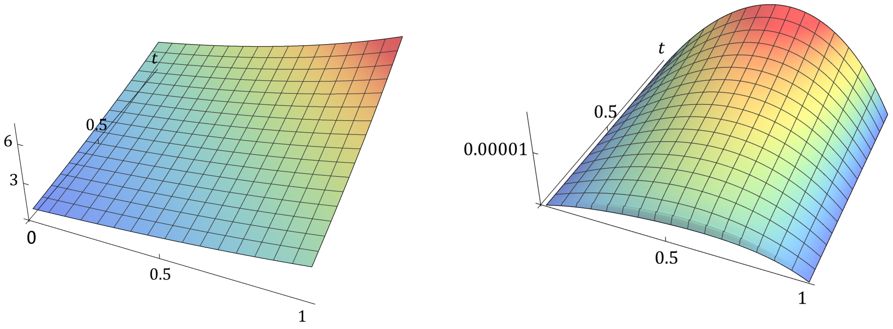
Equation (32) has the solution $u(x,t)=e^{x+t}$. The graphs of the numerical solution (29) for the subdiffusion Equation (32) and its error for $\alpha =0.5$, $L=1$, $h=0.02$, and $\tau =0.01$ are shown in Figure 1. The results of the numerical experiments for the error and the orders of convergence in time and space of the difference scheme (29) with $\alpha =0.25,0.5,0.75$ are presented in

Table 4. Error and order in time of difference scheme (29) of Equation (32) and $M=500$.

h	$\mathit{\alpha }=0.25$		$\mathit{\alpha }=0.5$		$\mathit{\alpha }=0.75$		CPU $\left(\mathbf{s}\right)$
	$\mathit{Error}$	$\mathit{Order}\left(\mathit{\tau }\right)$	$\mathit{Error}$	$\mathit{Order}\left(\mathit{\tau }\right)$	$\mathit{Error}$	$\mathit{Order}\left(\mathit{\tau }\right)$
$1/4$	$2.86\times {10}^{-3}$		$2.86\times {10}^{-3}$		$2.86\times {10}^{-3}$		$1.7187$
$1/8$	$7.18\times {10}^{-4}$	$1.9948$	$7.17\times {10}^{-4}$	$1.9948$	$7.18\times {10}^{-4}$	$1.9944$	$4.4843$
$1/16$	$1.81\times {10}^{-4}$	$1.9908$	$1.81\times {10}^{-4}$	$1.9909$	$1.81\times {10}^{-4}$	$1.9892$	$12.265$
$1/32$	$4.52\times {10}^{-5}$	$1.9995$	$4.52\times {10}^{-5}$	$1.9995$	$4.54\times {10}^{-5}$	$1.9929$	$36.437$
$1/64$	$1.12\times {10}^{-5}$	$2.0049$	$1.13\times {10}^{-5}$	$2.0025$	$1.15\times {10}^{-5}$	$1.9784$	$132.97$

and

Table 5. Error and order in space of difference scheme (29) of Equation (32) and $N=1000$.

h	$\mathit{\alpha }=0.25$		$\mathit{\alpha }=0.5$		$\mathit{\alpha }=0.75$		CPU (s)
	$\mathit{Error}$	$\mathit{Order}\left(\mathit{h}\right)$	$\mathit{Error}$	$\mathit{Order}\left(\mathit{h}\right)$	$\mathit{Error}$	$\mathit{Order}\left(\mathit{h}\right)$
$1/10$	$1.31\times {10}^{-4}$		$1.31\times {10}^{-4}$		$9.69\times {10}^{-4}$		$0.5156$
$1/20$	$3.14\times {10}^{-5}$	$2.0574$	$3.40\times {10}^{-5}$	$2.1067$	$2.28\times {10}^{-4}$	$2.0878$	$1.4687$
$1/40$	$7.66\times {10}^{-6}$	$2.0377$	$7.22\times {10}^{-6}$	$2.0736$	$5.49\times {10}^{-5}$	$2.0539$	$4.1406$
$1/80$	$1.88\times {10}^{-6}$	$2.0231$	$1.75\times {10}^{-6}$	$2.0418$	$1.34\times {10}^{-5}$	$2.0384$	$12.547$
$1/160$	$4.74\times {10}^{-7}$	$1.9915$	$4.31\times {10}^{-7}$	$2.0231$	$3.30\times {10}^{-6}$	$2.0179$	$42.234$

.

In the following, we prove that the difference scheme (29) with initial conditions (30) and (31) for the fractional subdiffusion equation is unconditionally stable and convergent with second-order accuracy. Denote by $E_n^m=u_n^m-U_n^m$ the errors of the difference scheme on the nodes of the grid $\mathcal{J}$. When $m>4$, the errors $E_n^m$ in row m of the grid $\mathcal{J}$ are the solutions of the system of linear equations $E_0^m=E_N^m=0$ and

$$-\eta E_{n-1}^m+(2\eta +{\omega }_0^{\left(\alpha \right)})E_n^m-\eta E_{n+1}^m={\mathcal{R}}_n^m.$$

From (28) and (29)

$${\mathcal{R}}_n^m=-\sum _{k=1}^{m-1}\left({\omega }_k^{\left(\alpha \right)}{E}_n^{m-k}\right)+\Gamma (2-\alpha )\left(A_n^m{\tau }^{2+\alpha }+B_n^m{\displaystyle \frac{{\tau }^2}{m^{\alpha }}}+D_n^m{\tau }^{\alpha }{h}^2\right).$$

(33)

Denote

$$M_i=max\left|{\displaystyle \frac{{\partial }^i}{\partial t^i}}u(x,t)\right|,{\tilde{M}}_4=max\left|{\displaystyle \frac{{\partial }^4}{\partial x^4}}u(x,t)\right|,$$

where the maximums are taken for all $(x,t)\in [0,1]\times [0,1]$ and the coefficients $A_n^m,B_n^m$ and $D_n^m$ satisfy the bounds

$$|A_n^m|<{\displaystyle \frac{252{\overline{M}}_3+45{\overline{M}}_4+2{\overline{M}}_5}{36\Gamma (4-\alpha )}},|B_n|<{\displaystyle \frac{{\overline{M}}_2}{12\Gamma (1-\alpha )}},|D_n^m|<{\displaystyle \frac{{\tilde{M}}_4}{12}}.$$

Let ${\mathcal{E}}_m$ be an $(N-1)$-dimensional vector whose entries are the errors $E_n^m$ of difference scheme (29) on row m of the grid $\mathcal{J}$, and let ${\mathcal{R}}_m$ be the vector of truncation errors (33). The system of equations for the errors of difference scheme (29) in row m of the grid $\mathcal{J}$ can be written in matrix form as

$$\mathcal{M}{\mathcal{E}}_m={\mathcal{R}}_m,$$

where $\mathcal{M}=\left(a_{i,j}\right)$ is a tridiagonal square matrix with nonzero entries

$$a_{i,i}=2\eta +{\omega }_0^{\left(\alpha \right)},a_{i-1,i}=a_{i+1,i}=-\eta ,(1\le i\le N-1).$$

(34)

The errors $E_n^1$ on the first row of $\mathcal{J}$ are solutions of the system of equations

$${\mathcal{M}}_1{\mathcal{E}}_1={\mathcal{R}}_1,$$

(35)

where the matrix ${\mathcal{M}}_1=\left(b_{i,j}\right)$ has nonzero entries

$$b_{i,i}=1+2{\eta }_1(1-\sigma ),b_{i-1,i}=b_{i+1,i}=-{\eta }_1(1-\sigma ),(1\le i\le N-1).$$

The errors on the second, third and fourth rows of $\mathcal{J}$ are solutions of the system of equations

$${\mathcal{M}}_0{\mathcal{E}}_m={\mathcal{R}}_m,(m=1,2,3),$$

(36)

where the matrix ${\mathcal{M}}_0=\left(c_{i,j}\right)$ has nonzero entries

$$c_{i,i}={\delta }_0^{\left(\alpha \right)}+2{\eta }_2{c}_0^{\sigma },c_{i-1,i}=c_{i+1,i}=-{\eta }_2{c}_0^{\sigma },(1\le i\le N-1).$$

The norms of ${\mathcal{R}}_m$ satisfy $\parallel {\mathcal{R}}_m\parallel <C_1{\tau }^{\alpha }({\tau }^2+h^2)$ for $m=1,2,3$ and 4. The matrices ${\mathcal{M}}_0$ and ${\mathcal{M}}_1$ are diagonally dominant. From the Ahlberg-Nilson-Varah bound their infinity norms satisfy the estimates [43,44]

$$\parallel {\mathcal{M}}_1^{-1}\parallel <1,\parallel {\mathcal{M}}_0^{-1}\parallel <{\displaystyle \frac{1}{{\delta }_0^{\left(\alpha \right)}}}.$$

Therefore

$$\parallel {\mathcal{E}}_1\parallel <\parallel {\mathcal{M}}_1^{-1}\parallel \parallel {\mathcal{R}}_1\parallel <C_1{\tau }^{\alpha }({\tau }^2+h^2),$$

$$\parallel {\mathcal{E}}_m\parallel <\parallel {\mathcal{M}}_0^{-1}\parallel \parallel {\mathcal{R}}_m\parallel <C_1{\tau }^{\alpha }({\tau }^2+h^2),$$

for $m=2,3$ and 4 because ${\delta }_0^{\left(\alpha \right)}=2{(2-\alpha /2)}^{1-\alpha }>1.$

Theorem 4. 

The errors of difference scheme (29) satisfy

$$\parallel {\mathcal{E}}_m\parallel <C({\tau }^2+h^2)$$

(37)

for all $m=1,\dots ,M$, where

$$C=max\left\{C_1,{\displaystyle \frac{6{\overline{M}}_2+252{\overline{M}}_3+45{\overline{M}}_4+2{\overline{M}}_5}{72(1-\alpha )}},{\displaystyle \frac{{\tilde{M}}_4}{12(1-\alpha )}}\right\}.$$

Proof. 

We prove the statement by induction. The estimate (37) holds for $m\le 4$. Assume that (37) holds for all rows $1,2,\dots ,m-1$ of the grid $\mathcal{J}$. From formula (33)

$$|{\mathcal{R}}_n^m| < -\sum _{k=1}^{m-1}{\omega }_k^{\left(\alpha \right)}|E_n^{m-k}|+\Gamma (2-\alpha )\left(|A_n^m|{\tau }^{2+\alpha }+|B_n^m|{\displaystyle \frac{{\tau }^2}{m^{\alpha }}}+|D_n^m|{\tau }^{\alpha }{h}^2\right).$$

When $0<\alpha <1$ the gamma function satisfies $0.88<\Gamma (2-\alpha )<1$ [45]. Applying the induction assumption

$$|{\mathcal{R}}_n^m| \le -\sum _{k=1}^{m-1}{\omega }_k^{\left(\alpha \right)}C({\tau }^2+h^2)+\Gamma (2-\alpha )|A_n^m|{\tau }^{2+\alpha }+\Gamma (2-\alpha )|B_n^m|{\displaystyle \frac{{\tau }^2}{m^{\alpha }}}+|D_n^m|{\tau }^2{h}^2,$$

$$|{\mathcal{R}}_n^m| < ({\omega }_0^{\left(\alpha \right)}-|{\omega }_m^{\left(\alpha \right)}|)C({\tau }^2+h^2)+A{\tau }^{2+\alpha }+{\displaystyle \frac{{\overline{M}}_2(1-\alpha )}{12}}{\displaystyle \frac{{\tau }^2}{m^{\alpha }}}+{\displaystyle \frac{{\tilde{M}}_4}{12}}{\tau }^{\alpha }{h}^2,$$

where $A<(252{\overline{M}}_3+45{\overline{M}}_4+2{\overline{M}}_5)/72$. From Proposition 6

$$|{\mathcal{R}}_n^m| < {\omega }_0^{\left(\alpha \right)}C({\tau }^2+h^2)-{\displaystyle \frac{1-a}{m^{\alpha }}}C({\tau }^2+h^2)+A{\displaystyle \frac{{\tau }^2}{m^{\alpha }}}+{\displaystyle \frac{{\overline{M}}_2(1-\alpha )}{12}}{\displaystyle \frac{{\tau }^2}{m^{\alpha }}}+{\displaystyle \frac{{\tilde{M}}_4}{12}}{\displaystyle \frac{h^2}{m^{\alpha }}},$$

$$|{\mathcal{R}}_n^m| < {\omega }_0^{\left(\alpha \right)}C({\tau }^2+h^2)-{\displaystyle \frac{(1-\alpha ){\tau }^2}{m^{\alpha }}}\left(C-{\displaystyle \frac{A}{1-\alpha }}-{\displaystyle \frac{{\overline{M}}_2}{12}}\right)-{\displaystyle \frac{(1-\alpha )h^2}{m^{\alpha }}}\left(C-{\displaystyle \frac{{\tilde{M}}_4}{12(1-\alpha )}}\right).$$

When C satisfies the conditions of the theorem, the two coefficients $C-A/(1-\alpha )-{\overline{M}}_2/12$ and $C-{\tilde{M}}_4/\left(12(1-\alpha )\right)$ are positive. Therefore

$$|{\mathcal{R}}_n^m| < {\omega }_0^{\left(\alpha \right)}C({\tau }^2+h^2).$$

From the Ahlberg-Nilson-Varah bound and (34) the infinity norm of ${\mathcal{M}}^{-1}$ satisfies [43,44]

$$\parallel {\mathcal{M}}^{-1}\parallel \le {\displaystyle \frac{1}{w_0^{\left(\alpha \right)}}}.$$

Hence

$${\mathcal{E}}_m={\mathcal{M}}^{-1}{\mathcal{R}}_m,$$

$$\parallel {\mathcal{E}}_m\parallel \le \parallel {\mathcal{M}}^{-1}\parallel \parallel {\mathcal{R}}_m\parallel <C({\tau }^2+h^2).$$

The error estimate (37) holds for the m-th row of the grid $\mathcal{J}$, completing the induction. □

5. Conclusions

In the present paper, we study the construction and properties of a parameter-dependent approximation for the second derivative, denoted by (7), and the approximations of the Caputo fractional derivative, denoted by (13) and (14), as well as their applications to the numerical solution of fractional differential equations. The approximations of the fractional derivative are developed using the second-order expansion formula of the L1 approximation together with the approximation (7) of the second derivative. The weights of the two resulting approximations of the fractional derivative satisfy property (2) when a suitable choice of the parameter is made. Approximation (13) of the fractional derivative has second-order accuracy, whereas the order of approximation (14) depends on the mesh size and ranges from $2-\alpha$ to two. We provide examples illustrating the application of the derived approximations to the construction of finite difference schemes for the numerical solution of fractional differential equations, and we analyze the convergence and accuracy of these numerical solutions. In Theorems 3 and 4, we prove that the difference schemes based on both approximations (13) and (14) achieve second-order accuracy. The proofs rely on property (2) of the approximation weights and on the magnitude of the final weights. The theoretical results for the convergence order and error of the proposed numerical methods are supported by the numerical experiments presented in the paper.

The methods for deriving the second-order expansion formula of the L1 approximation and the approximation (7) of the second derivative are generalized to arbitrary order and lead to three-point approximations of the Caputo fractional derivative [46]. In [47], we obtained an approximation of the fractional derivative that satisfies (2), and whose construction can also be extended to an arbitrary order. In future work, we will continue the investigation initiated in this paper and in [47] to construct high-order approximations of the fractional derivative. We will consider generalizations of approximation (14) for graded meshes, constructions of fast schemes, and their application to the numerical solution of fractional differential equations.

References

1. Alhajraf, A.; Yousef, A.; Bozkurt, F. An Analysis of a Fractional-Order Model of Colorectal Cancer and the Chemo-Immunotherapeutic Treatments with Monoclonal Antibody. Mathematics 2023, 11, 2374. [Google Scholar] [CrossRef]
2. Ghezal, A.; Al Ghafli, A.A.; Al Salman, H.J. Anomalous Drug Transport in Biological Tissues: A Caputo Fractional Approach with Non-Classical Boundary Modeling. Fractal Fract. 2025, 9, 508. [Google Scholar] [CrossRef]
3. Caputo, M.; Cametti, C. Fractional derivatives in the transport of drugs across biological materials and human skin. Physical A 2016, 462, 705–713. [Google Scholar] [CrossRef]
4. Fikl, A.; Jhinga, A.; Kaslik, E.; Mondal, A. Simulating neuronal dynamics in fractional adaptive exponential integrate-and-fire models. Fract. Calc. Appl. Anal. 2025, 28, 529–558. [Google Scholar] [CrossRef]
5. Sun, Z.Z.; Gao, G. Fractional Differential Equations: Finite Difference Methods; De Gruyter: Berlin, Germany, 2020; ISBN 978-3-11-061606-4. [Google Scholar]
6. Li, C.; Zeng, F. Finite Difference Methods for Fractional Differential Equations. Int. J. Bifurc. Chaos 2012, 22, 1230014. [Google Scholar] [CrossRef]
7. Podlubny, I. Fractional Differential Equations; Academic Press: San Diego, CA, USA, 1999. [Google Scholar]
8. Zayernouri, M.; Wang, L.-L.; Shen, J.; Karniadakis, G.E. Spectral and Spectral Element Methods for Fractional Ordinary and Partial Differential Equations; Cambridge University Press: Cambridge, UK, 2024. [Google Scholar]
9. Shi, X. Spectral Collocation Methods for Fractional Integro-Differential Equations with Weakly Singular Kernels. J. Sci. Comput. 2023, 94, 112. [Google Scholar] [CrossRef]
10. Ford, N.J.; Xiao, J.; Yan, Y. A Finite Element Method for Time Fractional Partial Differential Equations. Fract. Calc. Appl. Anal. 2011, 14, 454–474. [Google Scholar] [CrossRef]
11. Su, X.; Zhou, Y. A Fast High-Order Predictor–Corrector Method on Graded Meshes for Solving Fractional Differential Equations. Fractal Fract. 2022, 6, 516. [Google Scholar] [CrossRef]
12. Lubich, C. Discretized fractional calculus. SIAM J. Math. Anal. 1986, 17, 704–719. [Google Scholar] [CrossRef]
13. Dimitrov, Y.; Miryanov, R.; Todorov, V. Asymptotic Expansions and Approximations for the Caputo Derivative. Comput. Appl. Math. 2018, 37, 5476–5499. [Google Scholar] [CrossRef]
14. Jin, B.; Lazarov, R.; Zhou, Z. An analysis of the L1 scheme for the subdiffusion equation with nonsmooth data. IMA J. Numer. Anal. 2016, 36, 197–221. [Google Scholar] [CrossRef]
15. Li, B.; Xie, X.; Yan, Y. L1 scheme for solving an inverse problem subject to a fractional diffusion equation. Comput. Math. Appl. 2023, 134, 112–123. [Google Scholar] [CrossRef]
16. Scherer, R.; Kalla, S.L.; Tang, Y.; Huang, J. The Grünwald–Letnikov method for fractional differential equations. Comput. Math. Appl. 2011, 62, 902–917. [Google Scholar] [CrossRef]
17. Gao, G.-H.; Sun, Z.-Z.; Zhang, H.-W. A New Fractional Numerical Differentiation Formula to Approximate the Caputo Derivative and Its Applications. J. Comput. Phys. 2015, 259, 33–50. [Google Scholar] [CrossRef]
18. Alikhanov, A.A. A new difference scheme for the time fractional diffusion equation. J. Comput. Phys. 2015, 280, 424–438. [Google Scholar] [CrossRef]
19. Xiao, J.; Chen, Y.; Li; Zeng, F.; Zhang, Z. L1 Schemes for Time-Fractional Differential Equations: A Brief Survey and New Development. Numer. Math. Theory Methods Appl. 2025, 18, 544–574. [Google Scholar] [CrossRef]
20. Alikhanov, A.A.; Huang, C. A high-order L2 type difference scheme for the time fractional diffusion equation. Appl. Math. Comput. 2021, 411, 126545. [Google Scholar] [CrossRef]
21. Wang, Y.-M.; Ren, L. A high-order L2-compact difference method for Caputo-type time fractional sub-diffusion equations with variable coefficients. Appl. Math. Comput. 2019, 342, 71–93. [Google Scholar] [CrossRef]
22. Shams, M.; Carpentieri, B. Efficient families of higher-order Caputo-type numerical schemes for solving fractional order differential equations. Alexandria Eng. J. 2025, 124, 337–361. [Google Scholar] [CrossRef]
23. Luo, W.H.; Li, C.; Huang, T.Z.; Gu, X.M.; Wu, G.C. A High-Order Accurate Numerical Scheme for the Caputo Derivative with Applications to Fractional Diffusion Problems. Numer. Funct. Anal. Optim. 2017, 39, 600–622. [Google Scholar] [CrossRef]
24. Cai, M.; Li, C. Numerical Approaches to Fractional Integrals and Derivatives: A Review. Mathematics 2020, 8, 43. [Google Scholar] [CrossRef]
25. Gunarathna, W.A.; Nasir, H.M.; Daundasekera, W.B. An explicit form for higher order approximations of fractional derivatives. Appl. Numer. Math. 2019, 143, 51–60. [Google Scholar] [CrossRef]
26. Dimitrov, Y. Numerical approximations for fractional differential equations. J. Fract. Calc. Appl. 2014, 5, 1–45. [Google Scholar]
27. Hao, Z.-P.; Sun, Z.-Z.; Cao, W.-R. A fourth-order approximation of fractional derivatives with its applications. J. Comput. Phys. 2015, 281, 787–805. [Google Scholar] [CrossRef]
28. Dimitrov, Y.; Georgiev, S.; Todorov, V. First Derivative Approximations and Applications. Fractal Fract. 2024, 8, 608. [Google Scholar] [CrossRef]
29. Gu, X.-M.; Wu, S.-L. A Parallel-in-Time Iterative Algorithm for Volterra Partial Integro-Differential Problems with Weakly Singular Kernel. J. Comput. Phys. 2020, 417, 109576. [Google Scholar] [CrossRef]
30. Gong, C.; Bao, W.; Tang, G.; Jiang, Y.; Liu, J. A Parallel Algorithm for the Two-Dimensional Time Fractional Diffusion Equation with Implicit Difference Method. Sci. World J. 2014, 219580. [Google Scholar] [CrossRef]
31. Jiang, S.D.; Zhang, J.W.; Zhang, Q.; Zhang, Z.M. Fast Evaluation of the Caputo Fractional Derivative and Its Applications to Fractional Diffusion Equations. Commun. Comput. Phys. 2017, 21, 650–678. [Google Scholar] [CrossRef]
32. Yan, Y.G.; Sun, Z.Z.; Zhang, J.W. Fast Evaluation of the Caputo Fractional Derivative and Its Applications to Fractional Diffusion Equations: A Second-Order Scheme. Commun. Comput. Phys. 2017, 22, 1028–1048. [Google Scholar] [CrossRef]
33. Li, X.; Liao, H.L.; Zhang, L.M. A Second-Order Fast Compact Scheme with Unequal Time-Steps for Subdiffusion Problems. Numer. Algorithms 2021, 86, 1011–1039. [Google Scholar] [CrossRef]
34. Jiang, H.; Xu, D. A Fast High-Order Compact Difference Scheme for Time-Fractional KS Equation with the Generalized Burgers’ Type Nonlinearity. Fractal Fract. 2025, 9, 218. [Google Scholar] [CrossRef]
35. Liu, T.; Liu, H.; Ma, Y. Approximate Solution of a Kind of Time-Fractional Evolution Equations Based on Fast L1 Formula and Barycentric Lagrange Interpolation. Fractal Fract. 2024, 8, 675. [Google Scholar] [CrossRef]
36. Apostolov, S.; Dimitrov, Y.; Todorov, V. Constructions of second order approximations of the Caputo fractional derivative. In Large-Scale Scientific Computing. LSSC 2021; Lirkov, I., Margenov, S., Eds.; Lecture Notes in Computer Science; Springer: Berlin/Heidelberg, Germany, 2022; p. 13127. [Google Scholar]
37. Todorov, V.; Dimitrov, Y.; Dimov, I. Second order shifted approximations for the first derivative. In Advances in High Performance Computing. HPC 2019; Dimov, I., Fidanova, S., Eds.; Studies in Computational Intelligence; Springer: Cham, Switzerland, 2011; Volume 902. [Google Scholar]
38. Edwards, H.M. Riemann’s Zeta Function; Academic Press: New York, NY, USA, 1974. [Google Scholar]
39. Cao, J.; Xu, C. A high order scheme for the numerical solution of the fractional ordinary differential equations. J. Comput. Phys. 2013, 238, 154–168. [Google Scholar] [CrossRef]
40. Gülsu, M.; Öztürk, Y.; Anapalı, A. Numerical approach for solving fractional relaxation-oscillation equation. Appl. Math. Model. 2013, 37, 5927–5937. [Google Scholar] [CrossRef]
41. Langlands, T.A.M.; Henry, B.I. The accuracy and stability of an implicit solution method for the fractional diffusion equation. J. Comput. Phys. 2005, 205, 719–736. [Google Scholar] [CrossRef]
42. Dimitrov, Y.; Dimov, I.; Todorov, V. Numerical Solutions of Ordinary Fractional Differential Equations with Singularities. In Advanced Computing in Industrial Mathematics; Studies in Computational Intelligence; Springer: Cham, Switzerland, 2018; Volume 793, pp. 75–88. [Google Scholar] [CrossRef]
43. Kolotilina, L.Y. Bounds for the infinity norm of the inverse for certain M- and H-matrices. Linear Algebra Appl. 2009, 430, 692–702. [Google Scholar] [CrossRef]
44. Varah, J.M. A lower bound for the smallest singular value of a matrix. Linear Algebra Appl. 1975, 11, 3–5. [Google Scholar] [CrossRef]
45. Deming, W.; Colcord, C. The minimum in the gamma function. Nature 1935, 135, 917. [Google Scholar] [CrossRef]
46. Dimitrov, Y. Three-point approximation for the Caputo fractional derivative. Commun. Appl. Math. Comput. 2017, 31, 413–442. [Google Scholar]
47. Dimitrov, Y.; Georgiev, S.; Todorov, V. Approximation of Caputo Fractional Derivative and Numerical Solutions of Fractional Differential Equations. Fractal Fract. 2023, 7, 750. [Google Scholar] [CrossRef]
Figure 1. Graphs of the numerical solution of Equation (32)—(left) and the corresponding error—(right) for α = 0.5 , L = 1 , h = 0.02 , and τ = 0.01 .
Fractalfract 09 00816 g001