Quantized Nonfragile State Estimation of Memristor-Based Fractional-Order Neural Networks with Hybrid Time Delays Subject to Sensor Saturations

Abstract

This study addresses the issue of nonfragile state estimation for memristor-based fractional-order neural networks with hybrid randomly occurring delays. Considering the finite bandwidth of the signal transmission channel, quantitative processing is introduced to reduce network burden and prevent signal blocking and packet loss. In a real-world setting, the designed estimator may experience potential gain variations. To address this issue, a fractional-order nonfragile estimator is developed by incorporating a logarithmic quantizer, which ultimately improves the reliability of the state estimator. In addition, by combining the generalized fractional-order Lyapunov direct method with novel Caputo–Wirtinger integral inequalities, a lower conservative criterion is derived to guarantee the asymptotic stability of the augmented system. At last, the accuracy and practicality of the desired estimation scheme are demonstrated through two simulation examples.

1. Introduction

The origin of fractional calculus can be traced back to a question raised by L’Hôpital in 1695. Until a few decades ago, the available literature on fractional calculus primarily concentrated on theoretical analysis [1]. Commencing in 1960, the exploration of fractional calculus expanded its application to the realms of physics, science, and bioengineering, which received considerable attention [2,3,4]. As it turns out, fractional calculus can describe real phenomena more accurately than integer-order calculus due to its properties of infinite memory and heritability [5,6]. In recent years, research on fractional-order systems has received considerable attention from numerous scholars. A plethora of novel findings have been published on stability analysis, pinning control, synchronization, and other related topics [7,8,9]. For instance, the design of a nonfragile controller has been addressed in [10] for a class of delayed fraction-order uncertain systems. In addition, the authors in [11] addressed the $L_{\infty }$-gain problem of incommensurate fractional-order systems with hybrid time delays. What is striking is that the authors introduced a notable approach in stability analysis that relied on the solution’s monotonicity and positivity rather than a Lyapunov–Krasovskii functional.

It is worth noting that neural networks have become increasingly popular over the last few decades due to their wide applications in fault diagnosis, image recognition, signal processing, and more [12,13,14]. State estimation (SE) plays an important role in these applications. So far, a substantial body of research results on SE issues has been presented in the existing literature [15,16,17,18,19]. It is worth pointing out that these network structures are often analyzed and designed with resistors to simulate neural synapses. Note, that Chua introduced the concept of memristor in 1971 [20]. Unfortunately, it was not until 2008 that the first memristor component was produced by the HP Lab (as seen in [21]). Unlike conventional resistors, this unique type of resistor offers several advantages, including lower energy consumption, faster operation speed, and reduced memory space requirements. Hence, memristors have been applied in many complex systems, especially in neural networks, see [22,23,24]. In comparison to traditional neural networks with n neurons, the number of equilibria of memristor-based fractional-order neural networks increases from $2^n$ to $2^{2n^2+n}$, leading to a wide range of applications. Owing to these advantages, the dynamical analysis issues (e.g., dissipativity, stability, and synchronization) for fractional-order memristive neural networks (FOMNNs) have recently attracted considerable interest [25,26,27].

In contrast to the abundance of research findings on other dynamic analysis issues, there is a scarcity of literature addressing the SE issue specifically in the context of FOMNNs. Among the most available studies on the SE issue, the authors failed to consider the potential impact of gain variations in real-world scenarios [28,29,30]. The estimator gain perturbations from complex environments may lead to the fragility of the traditional estimator design. As a result, nonfragile techniques have drawn much attention for various types of network systems to withstand the influence of gain perturbations [31]. In [32], a nonfragile estimator was developed for delayed neural networks with randomly occurring nonlinearity. In [33], the study explored the nonfragile SE problem of delayed fractional-order neural networks under an event-triggered mechanism. The authors in [34] addressed the nonfragile SE issue of memristor-based fractional-order BAM neural networks with time-varying delays. However, the stability criterion derived is delay-independent. Quantitative processing has attracted significant attention as an efficient method for conserving network resources. In networked control systems, quantitative processing, such as compressing and decompressing sampled data, is frequently employed to minimize transmission load and preserve network resources. In [35], the authors addressed the problem of quantized SE for neural networks under cyber attacks. Despite this, there are few studies on designing a fractional-order nonfragile estimator for delayed FOMNNs, which serves as motivation for our research.

As is known, time delays always appear in real systems, which may impact the performance or stability [26,34]. Time delays typically result from various factors, such as limitations in the communication channel or bandwidth capacity. The common delays include discrete delay [11], distributed delay [36], leakage delay [25], and others, which have been addressed in numerous outstanding studies. For example, in [25], the Mittag–Leffler stability issue for neutral-type fractional-order neural networks with leakage delay was investigated. It is worth noting that in the context of random fluctuations in the real environment, time-varying delays may occur in a probabilistic manner, typically referred to as randomly occurring time-varying delays (ROTDs). For instance, the issue of partial-neurons-based SE for recurrent neural networks with ROTDs was examined in [15]. The discrete delay associated with a Bernoulli variable $\vartheta \left(t\right)$ was discussed. So far, there have been plenty of interesting findings on fractional-order neural networks with time delays. As far as we know, there is a lack of research on fractional-order neural networks with ROTDs, particularly in the context of neural networks based on memristors. Furthermore, the sensor output is often constrained by the inherent physical attributes of components, which may lead to saturated measurement outputs [37]. Furthermore, saturation may introduce nonlinear characteristics that could significantly impact the accuracy of the estimation algorithm. Considering the saturation as well as the time delay for FOMNNs is meaningful and practical and inspired by the aforementioned reasons, our aim is to investigate the nonfragile SE problem for a class of FOMNNs with ROTDs and sensor saturations. The key advantages of our investigation are outlined as follows:

(i) The nonfragile SE issue of memristor-based fractional-order neural networks is addressed subject to hybrid randomly occurring time-varying delays and sensor saturations.

(ii) In order to guarantee the asymptotic stability of the augmented system, a delay-dependent criterion has been derived using the Lyapunov theory. Different from the previous excellent results in [36,38,39], a Caputo–Wirtinger integral inequality is utilized to decrease conservatism.

(iii) Taking into account the finite bandwidth and potential gain variations, a fractional-order nonfragile estimator is developed with quantized measurements.

(iv) To validate the usefulness of the proposed estimation algorithm for FOMNNs, two numerical examples are provided.

2. Problem Formulation and Preliminaries

Several common definitions of fractional calculus have been presented, and some useful lemmas are recalled here.

Definition 1

([40]). The fractional integral operator of the function $\hslash \left(t\right)$ is defined by

$$\begin{array}{c}\hfill I^{\alpha }\hslash \left(t\right)=\frac{1}{\Gamma \left(\alpha \right)}{\int }_{t_0}^t{(t-\sigma )}^{\alpha -1}\hslash \left(\sigma \right)d\sigma ,\alpha \in {\mathbb{R}}^{+}\end{array}$$

(1)

where $t\ge t_0$ and the Gamma function $\Gamma \left(z\right)={\int }_0^{\infty }{e}^{-t}{t}^{z-1}dt$.

Definition 2

([40]). The Caputo’s derivative form of $\hslash \left(t\right)$ is

$$\begin{array}{c}\hfill {}_{t_0}{}^{C}D_t^{\alpha }\hslash \left(t\right)=\frac{1}{\Gamma (k-\alpha )}{\int }_{t_0}^t{(t-\sigma )}^{k-\alpha -1}{\hslash }^{\left(k\right)}\left(\sigma \right)d\sigma ,\end{array}$$

(2)

where $t\ge t_0$, and $\alpha \in (k-1,k),\hslash \left(t\right)\in C^k([t_0,\infty ),\mathbb{R})$.

In the follow-up, ${}_{t_0}{}^{C}D_t^{\alpha }$ with order $\alpha$ can be replaced by $D^{\alpha }$ on $[t_0,t]$. Then, consider the following FOMNNs model with hybrid time-varying delays:

$$\left\{\begin{array}{c}\begin{array}{cc}\hfill D^{\alpha }{\xi }_i\left(t\right)=& -c_i\left({\xi }_i\left(t\right)\right){\xi }_i\left(t\right)+\sum _{j=1}^n{a}_{ij}\left({\xi }_j\left(t\right)\right)f_j\left({\xi }_j\left(t\right)\right)+\gamma \left(t\right)\sum _{j=1}^n{b}_{ij}\left({\xi }_j\left(t\right)\right)f_j\left({\xi }_j(t-\varrho \left(t\right))\right)\hfill \\ & +\delta \left(t\right)\sum _{j=1}^n{e}_{ij}\left({\xi }_j\left(t\right)\right){\int }_{t-\mathfrak{d}\left(t\right)}^t{\mathsf{f}}_j\left({\xi }_j\left(s\right)\right)ds,\hfill \\ \hfill {\xi }_i\left(t_0\right)& ={\tilde{\phi }}_i\left(t_0\right),t_0\in [-\overline{\rho },0],\overline{\rho }=max\left\{\varrho ,\mathfrak{d}\right\},\hfill \end{array}\hfill \end{array}\right.$$

(3)

where $0<\alpha <1,{\xi }_i\left(t\right)$ is the ith neuron state; $c_i>0,f_j(·)$ represents the activation function, $\varrho \left(t\right),\mathfrak{d}\left(t\right)$ present time-varying transmission delays satisfying $0\le \varrho \left(t\right)\le \varrho ,0\le \mathfrak{d}\left(t\right)\le \mathfrak{d}$ and $\dot{\varrho }\left(t\right)\le \overline{\varrho }<1$ in which $\varrho ,d$ are known real constants. The state feedback positive matrix $c_i\left({\xi }_i\left(t\right)\right)$ and the memristive connection weights $a_{ij}\left({\xi }_j\left(t\right)\right),b_{ij}\left({\xi }_j\left(t\right)\right),e_{ij}\left({\xi }_j\left(t\right)\right)$ are described as follows:

$$\begin{array}{cc}\hfill & c_i\left({\xi }_i\left(t\right)\right)=\frac{1}{{\tilde{\mathcal{C}}}_i}\left[\sum _{j=1}^n({\tilde{\mathcal{W}}}_{ij}^a+{\tilde{\mathcal{W}}}_{ij}^b+{\tilde{\mathcal{W}}}_{ij}^e)\times sg{n}_{ij}+\frac{1}{{\mathcal{R}}_i}\right],a_{ij}\left({\xi }_j\left(t\right)\right)=\frac{{\tilde{\mathcal{W}}}_{ij}^a}{{\tilde{\mathcal{C}}}_i}\times sg{n}_{ij},\hfill \\ & b_{ij}\left({\xi }_j\left(t\right)\right)=\frac{{\tilde{\mathcal{W}}}_{ij}^b}{{\tilde{\mathcal{C}}}_i}\times sg{n}_{ij},e_{ij}\left({\xi }_j\left(t\right)\right)=\frac{{\tilde{\mathcal{W}}}_{ij}^e}{{\tilde{\mathcal{C}}}_i}\times sg{n}_{ij}\hfill \end{array}$$

where ${\tilde{\mathcal{W}}}_{ij}^a,{\tilde{\mathcal{W}}}_{ij}^b,{\tilde{\mathcal{W}}}_{ij}^e$ are the memductances of memristors $F_{aij},F_{aij}$ satisfying ${\tilde{\mathcal{W}}}_{ij}^a=\frac{1}{F_{aij}},{\tilde{\mathcal{W}}}_{ij}^b=\frac{1}{F_{bij}}$, ${\tilde{\mathcal{C}}}_i$ stands for the capacitor. $sg{n}_{ij}=1$ if $i\ne j,$ otherwise $-1$. According to the characteristics of $d_i\left({\xi }_i\left(t\right)\right),z_{ij}\left({\xi }_j\left(t\right)\right)$, we have

$$\begin{array}{c}\hfill c_i\left({\xi }_i\left(t\right)\right)=\left\{\begin{array}{c}{c}_i^{\prime },\left|{\xi }_i\left(t\right)\right|\le \mathfrak{T},\hfill \\ c_i^{″},\left|{\xi }_i\left(t\right)\right|>\mathfrak{T},\hfill \end{array}\right.z_{ij}\left({\xi }_j\left(t\right)\right)=\left\{\begin{array}{c}{z}_{ij}^{\prime },\left|{\xi }_j\left(t\right)\right|\le \mathfrak{T},\hfill \\ z_{ij}^{″},\left|{\xi }_j\left(t\right)\right|>\mathfrak{T},\hfill \end{array}\right.\end{array}$$

(4)

in which $\mathfrak{T}>0$ represents the switching jump, $c_i^{\prime },c_i^{″},z_{ij}^{\prime },z_{ij}^{″}$ are constants, and $c_i\left({\xi }_i\left(t\right)\right),z_{ij}\left({\xi }_j\left(t\right)\right)$ are switching by the states. The choice of state-dependent parameters are shown in the following Algorithm 1:

Algorithm 1: The Switching of Memristance Parameters

Input:  The constant value n, the initial value $i=1,j=1$. Output:  Obtain $c_i,a_{ij},b_{ij},e_{ij}$. while  $i\le n$  do $⌊\begin{array}{c}\mathbf{while}j\le n\mathbf{do}\hfill \\ ⌊\begin{array}{c}\mathbf{if}\left|{\xi }_i\left(t\right)\right|\le \mathfrak{T}\mathbf{then}\hfill \\ c_i=c_i^{\prime },a_{ij}=a_{ij}^{\prime },b_{ij}=b_{ij}^{\prime },e_{ij}=e_{ij}^{\prime }\hfill \\ \mathbf{else}\hfill \\ c_i=c_i^{″},a_{ij}=a_{ij}^{″},b_{ij}=b_{ij}^{″},e_{ij}=e_{ij}^{″}\hfill \\ j=j+1;\hfill \end{array}\hfill \\ i=i+1;\hfill \end{array}$

    According to the differential inclusions and set-valued maps [41], system (3) can be rewritten as

$$\begin{array}{cc}\hfill D^{\alpha }{\xi }_i\left(t\right)\in & -co\left\{c_i^{\prime },c_i^{″}\right\}{\xi }_i\left(t\right)+\sum _{j=1}^{n}co\left\{a_{ij}^{\prime },a_{ij}^{″}\right\}{f}_j\left({\xi }_j\left(t\right)\right)+\gamma \left(t\right)\sum _{j=1}^{n}co\left\{b_{ij}^{\prime },b_{ij}^{″}\right\}{f}_j\left({\xi }_j(t-\varrho \left(t\right))\right)\hfill \\ & +\delta \left(t\right)\sum _{j=1}^{n}co\left\{e_{ij}^{\prime },e_{ij}^{″}\right\}{\int }_{t-\mathfrak{d}\left(t\right)}^t{f}_j\left({\xi }_j\left(s\right)\right)ds,\hfill \end{array}$$

(5)

where $co\left\{c_i^{\prime },c_i^{″}\right\}=\left[{\underline{c}}_i,{\overline{c}}_i\right],co\left\{z_{ij}^{\prime },z_{ij}^{\prime }\right\}=\left[{\underline{z}}_{ij},{\overline{z}}_{ij}\right],$ with ${\underline{c}}_i=\min \left\{c_i^{\prime },c_i^{″}\right\},{\overline{c}}_i=\max \left\{{\mathrm{c}}_{\mathrm{i}}^{\prime },{\mathrm{c}}_{\mathrm{i}}^{″}\right\},{\underline{z}}_{ij}=\min \left\{{\mathrm{z}}_{\mathrm{ij}}^{\prime },{\mathrm{z}}_{\mathrm{ij}}^{″}\right\},{\overline{\mathrm{z}}}_{\mathrm{ij}}=\max \left\{{\mathrm{z}}_{\mathrm{ij}}^{\prime },{\mathrm{z}}_{\mathrm{ij}}^{″}\right\}$.

For presentation simplicity, we denote $\left[\underline{\mathcal{C}},\overline{\mathcal{C}}\right]={\left[{\underline{c}}_i,{\overline{c}}_i\right]}_{n\times n},\left[\underline{\mathcal{Z}},\overline{\mathcal{Z}}\right]={\left[{\underline{z}}_{ij},{\overline{z}}_{ij}\right]}_{n\times n},\xi \left(t\right)={\mathrm{col}}_n\left\{{\xi }_i\left(t\right)\right\},f\left(\xi \left(t\right)\right)={\mathrm{col}}_n\left\{f_j\left({\xi }_j\left(t\right)\right)\right\},f\left(\xi (t-{\varrho }_t)\right)={\mathrm{col}}_n\left\{f_j\left({\xi }_j(t-\varrho \left(t\right))\right)\right\}$. Then, system (5) can be represented in matrix form as

$$\begin{array}{c}\hfill D^{\alpha }\xi \left(t\right)=-{\mathcal{C}}^{★}\xi \left(t\right)+{\mathcal{A}}^{★}g\left(\xi \left(t\right)\right)+\gamma \left(t\right){\mathcal{B}}^{★}f\left(\xi (t-{\varrho }_t)\right)+\delta \left(t\right){\mathcal{E}}^{★}{\int }_{t-\mathfrak{d}\left(t\right)}^{t}f\left(\xi \left(s\right)\right)ds,\end{array}$$

(6)

where ${\mathcal{C}}^{★}\in \left[\underline{\mathcal{C}},\overline{\mathcal{C}}\right],{\mathcal{Z}}^{★}\in \left[\underline{\mathcal{Z}},\overline{\mathcal{Z}}\right]$ are measurable functions. By means of Lemma 1 in [42], neural network model (6) is further rewritten as

$$\begin{array}{cc}\hfill D^{\alpha }\xi \left(t\right)=& -\overrightarrow{\mathcal{C}}\xi \left(t\right)+\overrightarrow{\mathcal{A}}f\left(\xi \left(t\right)\right)+\gamma \left(t\right)\overrightarrow{\mathcal{B}}f\left(\xi (t-\varrho \left(t\right))\right)+\delta \left(t\right)\overrightarrow{\mathcal{E}}{\int }_{t-\mathfrak{d}\left(t\right)}^{t}f\left(\xi \left(s\right)\right)ds,\hfill \end{array}$$

(7)

where $\overrightarrow{\mathcal{C}}={\mathcal{C}}^{\prime }+\Delta \mathcal{C},$$\overrightarrow{\mathcal{Z}}={\mathcal{Z}}^{\prime }+\Delta \mathcal{Z},$${\mathcal{C}}^{\prime }=\frac{\underline{\mathcal{C}}+\overline{\mathcal{C}}}{2},$$\Delta \mathcal{C}={\mathcal{H}}_c{\mathcal{F}}_c\left(t\right){\mathcal{N}}_c,$${\mathcal{Z}}^{\prime }=\frac{\underline{\mathcal{Z}}+\overline{\mathcal{Z}}}{2},$$\mathcal{Z}={\mathcal{H}}_z{\mathcal{F}}_z\left(t\right){\mathcal{N}}_z,$ with ${\mathcal{F}}_{\mathrm{c}}^{\mathrm{T}}\left(\mathrm{t}\right){\mathcal{F}}_{\mathrm{c}}\left(\mathrm{t}\right)\le {\mathcal{I}}_{{\mathrm{n}}^2},$${\mathcal{F}}_{\mathrm{z}}^{\mathrm{T}}\left(\mathrm{t}\right){\mathcal{F}}_{\mathrm{z}}\left(\mathrm{t}\right)\le {\mathcal{I}}_{{\mathrm{n}}^2},$${\mathcal{H}}_{\mathrm{c}}=\left[{\mathcal{H}}_{\mathrm{c}1},{\mathcal{H}}_{\mathrm{c}2},\cdots ,{\mathcal{H}}_{\mathrm{cn}}\right],$${\mathcal{F}}_{\mathrm{c}}\left(\mathrm{t}\right)=\mathrm{diag}\left\{\underset{\ell -1}{\underbrace{0,\cdots ,0}},{\mathcal{F}}_{\mathrm{c}\ell }\left(\mathrm{t}\right),\underset{\mathrm{n}-\ell }{\underbrace{0,\cdots ,0}}\right\},$${\mathcal{H}}_{\mathrm{z}}=\left[{\mathcal{H}}_{\mathrm{z}1},{\mathcal{H}}_{\mathrm{z}2},\cdots ,{\mathcal{H}}_{\mathrm{zn}}\right],$${\mathcal{F}}_{\mathrm{z}}\left(\mathrm{t}\right)=\left\{{\mathcal{F}}_{\mathrm{z}11}\left(\mathrm{t}\right),{\mathcal{F}}_{\mathrm{z}12}\left(\mathrm{t}\right),\cdots ,{\mathcal{F}}_{znn}\left(t\right)\right\},$${\mathcal{N}}_c={\mathcal{N}}_z={\underset{n}{\underbrace{\left[{\mathcal{I}}_n,{\mathcal{I}}_n,\cdots ,{\mathcal{I}}_n\right]}}}^T$.

Remark 1.

Taking the phenomena of RODs into consideration, two stochastic variables $\gamma \left(t\right),\delta \left(t\right)$ which obey the Bernoulli distribution are employed and satisfy the following statistical properties: $Pr\left\{\gamma \left(t\right)=1\right\}=\mathcal{E}\left\{\gamma \left(t\right)\right\}=\overline{\gamma },Pr\left\{\gamma \left(t\right)=0\right\}=1-\overline{\gamma },Pr\left\{\delta \left(t\right)=1\right\}=\mathcal{E}\left\{\delta \left(t\right)\right\}=\overline{\delta },Pr\left\{\delta \left(t\right)=0\right\}=1-\overline{\delta }$. Furthermore, analyzing the dynamic behaviors of FOMNNs is challenging due to the state-dependent nature of memristive connection weights. As is it known that the traditional methods for addressing the stability and SE of NNs are not applicable to memristor-based FONNs. Different from the existing excellent results [43,44,45], in this paper, we transform FOMNNs (3) into a class of uncertain systems.

Assumption 1.

The function $f(·):{\mathbb{R}}^n\to {\mathbb{R}}^n$ satisfies $f\left(0\right)=0$ and the following sector-bounded condition:

$$\begin{array}{c}\hfill {\left[f\left({\nu }_1\right)-f\left({\nu }_2\right)-{\overrightarrow{F}}_1({\nu }_1-{\nu }_2)\right]}^T\left[f\left({\nu }_1\right)-f\left({\nu }_2\right)-{\overrightarrow{F}}_2({\nu }_1-{\nu }_2)\right]\le 0,\end{array}$$

(8)

in which $\forall {\nu }_1,{\nu }_2\in {\mathbb{R}}^n$, matrices ${\overrightarrow{F}}_1$ and ${\overrightarrow{F}}_2$ are known.

The measurement outputs ${\vartheta }_s\left(t\right)$ are as follows:

$$\begin{array}{cc}\hfill {\vartheta }_s\left(t\right)=& \mathfrak{S}\left(\vartheta \right(t\left)\right),\hfill \end{array}$$

(9)

$$\begin{array}{cc}\hfill \vartheta \left(t\right)=& \mathcal{C}\xi \left(t\right)\hfill \end{array}$$

(10)

where $\vartheta \left(t\right)$ represents the output vector. $\mathcal{C}$ is known constant matrices with appropriate dimensions. The function $\mathfrak{S}(·):{\mathbb{R}}^n\to {\mathbb{R}}^n$ is a saturation function defined as follows:

$$\begin{array}{c}\hfill \mathfrak{S}\left(\vartheta \right)\triangleq {\left[{\mathfrak{S}}_1^T\left({\vartheta }_1\right),{\mathfrak{S}}_2^T\left({\vartheta }_2\right),\cdots {\mathfrak{S}}_n^T\left({\vartheta }_n\right)\right]}^T\end{array}$$

where ${\mathfrak{S}}_{\ell }\left({\vartheta }_{\ell }\right)\triangleq \mathrm{sign}\left({\vartheta }_{\ell }\right)min\left\{{\vartheta }_{\ell ,\max },\left|{\vartheta }_{\ell }\right|\right\}(\ell =1,2,\cdots ,n)$ with ${\vartheta }_{\ell ,\max }$ being the ℓth element of ${\vartheta }_{max}$ (i.e., the saturation level).

In many practical problems, the estimator gains $\mathcal{K}$ may undergo certain adjustments or fluctuations due to the complex and changeable environment, which can result in system fragility [32]. Hence, it is necessary to design a fractional-order nonfragile estimator to reduce the influence of gain variation.

$$\left\{\begin{array}{c}\begin{array}{cc}\hfill D^{\alpha }\hat{\xi }\left(t\right)=& -{\mathcal{C}}^{\prime }\hat{\xi }\left(t\right)+{\mathcal{A}}^{\prime }f\left(\hat{\xi }\left(t\right)\right)+\overline{\gamma }{\mathcal{B}}^{\prime }f\left(\hat{\xi }(t-{\varrho }_t)\right)+\overline{\delta }{\mathcal{E}}^{\prime }{\int }_{t-\mathfrak{d}\left(t\right)}^{t}f\left(\xi \left(s\right)\right)ds\hfill \\ & +(\mathcal{K}+\Delta \mathcal{K})({\vartheta }_s\left(t\right)-\hat{\vartheta }\left(t\right)),\hfill \\ \hfill \hat{\vartheta }\left(t\right)=& \mathcal{C}\hat{\xi }\left(t\right),\hfill \end{array}\hfill \end{array}\right.$$

(11)

where $\hat{\xi }\left(t\right)$ denotes the estimation of $\xi \left(t\right)$, and $\mathcal{K}$ is the estimator gain to be designed. $\Delta \mathcal{K}$ signifies the fluctuation with ${\mathcal{H}}_k{\mathcal{F}}_k\left(t\right){\mathcal{N}}_k,{\mathcal{F}}_k^T\left(t\right){\mathcal{F}}_k\left(t\right)\le \mathcal{I}$. In addition, considering the effect of quantization in [35,46], we introduce the quantitative process to save the bandwidth and the logarithmic quantizer $\mathfrak{Q}\left(z\right)=\mathrm{col}\left\{{\mathfrak{Q}}_1\left(z_1\right),{\mathfrak{Q}}_2\left(z_2\right),\cdots ,{\mathfrak{Q}}_m\left(z_m\right)\right\}$ is employed with

$$\begin{array}{c}\hfill {\mathfrak{Q}}_l\left({\varkappa }_l\right)=\left\{\begin{array}{c}{\upsilon }^i{u}_0,\frac{{\upsilon }^i{u}_0}{1+ϵ}<{\varkappa }_l\le \frac{{\upsilon }^i{u}_0}{1-ϵ},i=0,\pm 1,\pm 2,\cdots ,\hfill \\ 0,{\varkappa }_l=0,\hfill \\ -\mathfrak{Q}(-{\varkappa }_l),{\varkappa }_l<0\hfill \end{array}\right.\end{array}$$

(12)

where $0<\upsilon <1$ denotes the quantization density, $u_0$ is a scaling scalar, $ϵ=\frac{1-\upsilon }{1+\upsilon }$. As observed in [47], $\mathfrak{Q}\left(\varkappa \right)$ can be rewritten as

$$\begin{array}{c}\hfill {\vartheta }_{\mathrm{q}}\left(t\right)\triangleq \mathfrak{Q}\left(\varkappa \right)=(\mathcal{I}+\Delta \iota )\varkappa ,\end{array}$$

(13)

where $-ϵ\le \Delta {\iota }_i\le ϵ$.

Next, define $\nu \left(t\right)=\xi \left(t\right)-\hat{\xi }\left(t\right)$ and $\tilde{f}\left(\nu \left(t\right)\right)=f\left(\xi \left(t\right)\right)-f\left(\hat{\xi }\left(t\right)\right)$. The error dynamic is shown as

$$\begin{array}{cc}\hfill D^{\alpha }\nu \left(t\right)=& -{\mathcal{C}}^{\prime }\nu \left(t\right)-\Delta \mathcal{C}\xi \left(t\right)+{\mathcal{A}}^{\prime }\tilde{f}\left(\nu \left(t\right)\right)+\Delta \mathcal{A}f\left(\xi \left(t\right)\right)+\overline{\gamma }{\mathcal{B}}^{\prime }\tilde{f}\left(\nu (t-{\varrho }_t)\right)\hfill \\ & +\overline{\gamma }\Delta \mathcal{B}f\left(\xi (t-{\varrho }_t)\right)\overline{\delta }{\mathcal{E}}^{\prime }{\int }_{t-\mathfrak{d}\left(t\right)}^t\tilde{f}\left(\nu \left(s\right)\right)ds+\overline{\delta }\Delta \mathcal{E}{\int }_{t-\mathfrak{d}\left(t\right)}^{t}f\left(\xi \left(s\right)\right)ds\hfill \\ & -(\mathcal{K}+\Delta \mathcal{K})\left({\vartheta }_{\mathrm{q}}\left(t\right)-\mathcal{C}\xi \left(t\right)+\mathcal{C}\nu \left(t\right)\right)+\varsigma \left(t\right),\hfill \end{array}$$

(14)

where $\varsigma \left(t\right)=\tilde{\gamma }({\mathcal{B}}^{\prime }+\Delta \mathcal{B})f\left(\xi (t-\varrho \left(t\right))\right)+\tilde{\delta }({\mathcal{E}}^{\prime }+\Delta \mathcal{E}){\int }_{t-\mathfrak{d}\left(t\right)}^{t}f\left(\xi \left(s\right)\right)ds,\tilde{\gamma }=\gamma \left(t\right)-\overline{\gamma }$, $\tilde{\delta }=\delta \left(t\right)-\overline{\delta }$.

Definition 3

([48]). A nonlinearity $\mathfrak{S}(·)$ is said to satisfy a sector condition if

$$\begin{array}{c}\hfill {(\mathfrak{S}\left(x\right)-{\mathcal{G}}_{1}x)}^T(\mathfrak{S}\left(x\right)-{\mathcal{G}}_{2}x)\le 0,\forall x\in {\mathbb{R}}^n.\end{array}$$

(15)

for real matrices ${\mathcal{G}}_1\in {\mathbb{R}}^{n\times n}$ and ${\mathcal{G}}_2\in {\mathbb{R}}^{n\times n}$ with ${\mathcal{G}}_1\le 0,{\mathcal{G}}_2\le 0,\mathcal{G}={\mathcal{G}}_2-{\mathcal{G}}_1>0$. In this case, the nonlinear function $\mathfrak{S}(·)$ can be said to belong to the sector $[{\mathcal{G}}_1,{\mathcal{G}}_2].$

From (15), the nonlinear function $\mathfrak{S}(·)$ can be rewritten as

$$\begin{array}{c}\hfill \mathfrak{S}\left(\mathcal{C}\xi \left(t\right)\right)={\mathcal{G}}_1\mathcal{C}\xi \left(t\right)+\chi \left(\mathcal{C}\xi \left(t\right)\right),\end{array}$$

(16)

Then, the nonlinearity $\chi (·)\in Y$ satisfies

$$\begin{array}{c}\hfill Y\triangleq \left\{\chi :{\chi }^T\left(\mathcal{C}\xi \left(t\right)\right)(\chi \left(\mathcal{C}\xi \left(t\right)\right)-\mathcal{G}\mathcal{C}\xi \left(t\right))\le 0\right\},\end{array}$$

(17)

In what follows, letting $\overrightarrow{\nu }\left(t\right)\triangleq \mathrm{col}\left\{\xi \left(t\right),\nu \left(t\right)\right\},{\phi }_f\left(t\right)\triangleq \mathrm{col}\left\{f\left(t\right),\tilde{f}\left(\nu \left(t\right)\right)\right\},{\phi }_f(t-{\varrho }_t)\triangleq \mathrm{col}\left\{f(t-\varrho \left(t\right)),\tilde{f}(t-\varrho \left(t\right))\right\}$, the augmented system can be obtained from (7) and (14):

$$\begin{array}{cc}\hfill D^{\alpha }\overrightarrow{\nu }\left(t\right)=& \tilde{\mathcal{C}}\overrightarrow{\nu }\left(t\right)+\tilde{\mathcal{A}}{\phi }_f\left(t\right)+\overline{\gamma }\tilde{\mathcal{B}}{\phi }_f(t-{\varrho }_t))-{\tilde{\mathcal{K}}}^{\prime }(\mathcal{I}+\Delta \iota )\chi \left(\overline{\mathcal{C}}\overrightarrow{\nu }\left(t\right)\right)\hfill \\ & +\overline{\delta }\tilde{\mathcal{E}}{\int }_{t-\mathfrak{d}\left(t\right)}^t{\phi }_f\left(s\right)ds+\tilde{\varsigma }\left(t\right),\hfill \end{array}$$

(18)

where $\tilde{\mathcal{C}}=\left[\begin{array}{cc}-{\mathcal{C}}^{\prime }-\Delta \mathcal{C}& 0\\ -\Delta \mathcal{C}-\tilde{\mathcal{K}}(\mathcal{I}+\Delta \iota ){\mathcal{G}}_1\mathcal{C}-\tilde{\mathcal{K}}\mathcal{C}& -{\mathcal{C}}^{\prime }-\tilde{\mathcal{K}}{\mathcal{G}}_1{\mathcal{C}}_1\end{array}\right],\tilde{\mathcal{Z}}=\left[\begin{array}{cc}{\mathcal{Z}}^{\prime }+\Delta \mathcal{Z}& 0\\ \Delta \mathcal{Z}& {\mathcal{Z}}^{\prime }\end{array}\right],{\tilde{\mathcal{K}}}^{\prime }=\left[\begin{array}{c}0\\ \tilde{\mathcal{K}}\end{array}\right]$, $\widetilde{{\mathcal{B}}_1}=\left[\begin{array}{cc}0& 0\\ \overrightarrow{\mathcal{B}}& 0\end{array}\right]$, $\widetilde{{\mathcal{E}}_1}=\left[\begin{array}{cc}0& 0\\ \overrightarrow{\mathcal{E}}& 0\end{array}\right]$, $\tilde{\varsigma }\left(t\right)=\tilde{\gamma }{\mathcal{B}}_1{\phi }_f(t-{\varrho }_t)+\tilde{\delta }{\mathcal{E}}_1{\int }_{t-\mathfrak{d}\left(t\right)}^t{\phi }_f\left(s\right)ds$, $\tilde{\mathcal{K}}=\mathcal{K}+\Delta \mathcal{K},\overline{\mathcal{C}}=[\mathcal{C} 0].$

Lemma 1

([49]). Let the function $\overrightarrow{\nu }\left(t\right)\in R^n$ be continuous and differential. Then, one has

$$\begin{array}{c}\hfill \frac{1}{2}{D}^{\alpha }{\overrightarrow{\nu }}^T\left(t\right)\mathcal{Q}\overrightarrow{\nu }\left(t\right)\le {\overrightarrow{\nu }}^T\left(t\right)\mathcal{Q}{D}^{\alpha }\overrightarrow{\nu }\left(t\right),\forall \alpha \in (0,1)\end{array}$$

Lemma 2

([50]). Let $\overrightarrow{\nu }:[\varrho ,{\varrho }_2]\in {\mathbb{R}}^{+}\to {\mathbb{R}}^n$ be differentiable. There exist positive symmetric matrix $\mathcal{O}>0$, and matrices ${\mathfrak{L}}_1,{\mathfrak{L}}_2,{\mathfrak{L}}_3\in {\mathbb{R}}^{3n\times n}$ satisfying the following relationship:

$$\begin{array}{c}\hfill -{\int }_{\varrho }^{{\varrho }_2}{\left(D^{\alpha }\overrightarrow{\nu }\left(\zeta \right)\right)}^T\mathcal{O}{D}^{\alpha }\overrightarrow{\nu }\left(\zeta \right)d\zeta \le {\Theta }^T\Phi \Theta ,m-1<\alpha <m\end{array}$$

where

$$\begin{array}{cc}\hfill \Phi =& ({\varrho }_2-\varrho )\left({\mathfrak{L}}_1{\mathcal{O}}^{-1}{\mathfrak{L}}_1^T+\frac{1}{3}{\mathfrak{L}}_2{\mathcal{O}}^{-1}{\mathfrak{L}}_2^T+\frac{1}{5}{\mathfrak{L}}_3{\mathcal{O}}^{-1}{\mathfrak{L}}_3^T\right)\hfill \\ & +\mathrm{sym}\left\{{\mathfrak{L}}_1{g}_1+{\mathfrak{L}}_2(g_1-2g_2)+M_3(g_1-6g_2+6g_3)\right\},\hfill \\ \hfill \Theta =& \mathrm{col}\{{\int }_{\varrho }^{{\varrho }_2}\left(D^{\alpha }\overrightarrow{\nu }\left(\zeta \right)\right)d\zeta ,\frac{1}{{\varrho }_2-\varrho }{\int }_{\varrho }^{{\varrho }_2}{\int }_{\varrho }^{\zeta }\left(D^{\alpha }\overrightarrow{\nu }\left(\rho \right)\right)d\rho d\zeta ,\hfill \\ & \frac{2}{{({\varrho }_2-\varrho )}^2}{\int }_{\varrho }^{{\varrho }_2}{\int }_{\varrho }^{\zeta }{\int }_{\varrho }^r{D}^{\alpha }\overrightarrow{\nu }\left(\rho \right)d\rho drd\zeta \},\hfill \end{array}$$

Definition 4

([50]). Assume that a Lyapunov function $\mathbb{V}(t,{\overrightarrow{\nu }}_t)$ and a class $-\mathcal{K}$ functions ${\delta }_i(i=1,2,3)$ satisfy

$$\begin{array}{c}\hfill {\delta }_1\parallel \overrightarrow{\nu }\parallel \le \mathbb{V}(t,{\overrightarrow{\nu }}_t)\le {\delta }_2\parallel \overrightarrow{\nu }\parallel ,\\ \hfill {}_0{}^{C}D^{\alpha }\mathbb{V}(t,{\overrightarrow{\nu }}_t)\le -{\delta }_3{\parallel \overrightarrow{\nu }\parallel }^b+c{t}^{-\alpha },\end{array}$$

where $0<\alpha <1,c>0$ is an arbitrary constant. Then, the fractional-order system (18) is asymptotically stable.

3. Main Results

For brevity, we establish the following associated notations:

$$\begin{array}{cc}\hfill \overrightarrow{\zeta }\left(t\right)=\mathrm{col}\{& \overrightarrow{\nu }\left(t\right),\overrightarrow{\nu }(t-{\varrho }_t),\overrightarrow{\nu }(t-\varrho ),{}_0{}^{C}D_t^{\alpha }\overrightarrow{\nu }\left(t\right),{\phi }_f\left(t\right),{\phi }_f(t-{\varrho }_t),{\int }_{t-\mathfrak{d}\left(t\right)}^t{\phi }_f\left(s\right)ds\hfill \\ & \varpi \left(t\right),\chi \left(\overline{\mathcal{C}}\overrightarrow{\nu }\left(t\right)\right)\},\hfill \\ \hfill \varpi \left(t\right)=\mathrm{col}\{& {\int }_{t-\varrho }^t{}_0{}^{C}D_t^{\alpha }\overrightarrow{\nu }\left(\zeta \right)d\zeta ,{\int }_{t-\varrho }^t{\int }_{t-\varrho }^s{}_0{}^{C}D_t^{\alpha }\overrightarrow{\nu }\left(\zeta \right)d\zeta ds,\vartheta \left(t\right)\},\hfill \\ \hfill \vartheta \left(t\right)={\int }_{t-\varrho }^t& {\int }_{t-\varrho }^s{\int }_{t-\varrho }^u{}_0{}^{C}D_t^{\alpha }\overrightarrow{\nu }\left(\zeta \right)d\zeta dsdu,\hfill \end{array}$$

Theorem 1.

Let the estimator gain matrix $\mathcal{K}$ be given, and let $\Delta \mathcal{K}$ be known. For given positive scalars $\varrho ,d$, the augmented system (18) is stochastically asymptotically stable if there are definite matrices $\mathcal{P},{\mathcal{Q}}_{\ell }(\ell =1,2),\mathcal{O},\mathcal{R}$, any matrix ${\mathfrak{L}}_1,{\mathfrak{L}}_2,{\mathfrak{L}}_3,{\mathcal{W}}_l(l=1,2)$ and three positive scalars ${\kappa }_1,{\kappa }_2,{\kappa }_3$ such that

$$\begin{array}{c}\hfill \mho =\left[\begin{array}{cccc}{\rm Y}& \sqrt{\varrho }{\tilde{\mathfrak{L}}}_1& \sqrt{\varrho }{\tilde{\mathfrak{L}}}_2& \sqrt{\varrho }{\tilde{\mathfrak{L}}}_3\\ *& -\mathcal{O}& 0& 0\\ *& *& -3\mathcal{O}& 0\\ *& *& *& -5\mathcal{O}\end{array}\right]<0,\end{array}$$

(19)

where ${\rm Y}=\left[\begin{array}{ccc}{\Xi }_1& {\Xi }_2& {\Re }_1\\ *& {\Xi }_3& {\Re }_2\\ *& *& {\Xi }_4\end{array}\right]$,  ${\Xi }_1=\left[\begin{array}{cccc}{\Pi }_{1,1}& 0& 0& {\Pi }_{1,4}\\ *& {\Pi }_{2,2}& 0& 0\\ *& *& {\Pi }_{3,3}& 0\\ *& *& *& {\Pi }_{4,4}\end{array}\right],$${\Xi }_2=\left[\begin{array}{ccc}{\Pi }_{1,5}& {\Pi }_{1,6}& {\Pi }_{1,7}\\ 0& {\Pi }_{2,6}& 0\\ 0& 0& 0\\ {\Pi }_{4,5}& {\Pi }_{4,6}& {\Pi }_{4,7}\end{array}\right],$${\Xi }_3=\mathrm{diag}\left\{-{\kappa }_1\mathcal{I}+d^2\mathcal{R},-{\kappa }_2\mathcal{I},-\mathcal{R}\right\},$${\Pi }_{1,1}={\mathcal{Q}}_1+{\mathcal{Q}}_2-{\kappa }_1{\mathfrak{J}}_1-\mathrm{sym}\left\{{\mathcal{W}}_1\tilde{\mathcal{C}}\right\},$${\Pi }_{1,9}=-{\mathcal{W}}_1{\tilde{\mathcal{K}}}^{\prime }(\mathcal{I}+{\Delta }_{\iota }),$${\Pi }_{1,5}={\mathcal{W}}_1\tilde{\mathcal{A}}-{\kappa }_1{\mathfrak{J}}_1,$${\Pi }_{1,6}=\overline{\gamma }{\mathcal{W}}_1\tilde{\mathcal{B}},$${\Pi }_{1,7}=\overline{\delta }{\mathcal{W}}_1\tilde{\mathcal{E}},$${\Pi }_{1,4}=\mathcal{P}-{\mathcal{W}}_1+{\tilde{\mathcal{C}}}^T{\mathcal{W}}_2,$${\Pi }_{3,3}=-{\mathcal{Q}}_1,$${\Pi }_{4,4}=\varrho \mathcal{O}-2{\mathcal{W}}_2,$${\Pi }_{4,7}=\overline{\delta }{\mathcal{W}}_2\mathcal{E},$${\Pi }_{4,5}={\mathcal{W}}_2\tilde{\mathcal{A}},$${\Pi }_{4,6}=\overline{\gamma }{\mathcal{W}}_2\tilde{\mathcal{B}},$${\Pi }_{4,9}=-{\mathcal{W}}_2(\mathcal{I}+{\Delta }_{\iota }),$${\Pi }_{2,2}=-{\kappa }_2{\mathfrak{J}}_1-(1-\overline{\varrho }){\mathcal{Q}}_2,$${\Pi }_{2,6}=-{\kappa }_2{\mathfrak{J}}_2,$${\Pi }_{6,6}=-{\kappa }_2\mathcal{I},$${\Pi }_{4,9}=-{\mathcal{W}}_2{\tilde{\mathcal{K}}}^{\prime }(\mathcal{I}+{\Delta }_{\iota }),$${\Pi }_{9,9}=-2{\kappa }_3\mathcal{I},$${\Pi }_{1,9}={\overline{\mathcal{C}}}^T{\mathcal{G}}^T,$${\Re }_1=\left[0{\Omega }_1\right],$${\Re }_2=\left[0{\Omega }_2\right],$${\Omega }_1={\left[{\Pi }_{1,9}^{T}00\right]}^T,$${\Omega }_2={\left[0{\Pi }_{4,9}^{T}00\right]}^T,$${\tilde{\mathfrak{L}}}_i={\left[0000000{\mathfrak{L}}_i^T\right]}^T,$${\Xi }_4=\left[\omega 0;0{\Pi }_{9,9}\right],$$\omega =\mathrm{sym}\left\{{\mathfrak{L}}_1{g}_1+{\mathfrak{L}}_2(g_1-2g_2)+{\mathfrak{L}}_3(g_1-6g_2+6g_3)\right\},$${\Pi }_{9,9}=-2{\kappa }_3\mathcal{I},$${\mathfrak{J}}_1={\mathrm{diag}}_2\left\{\mathcal{I}\otimes \frac{{\overrightarrow{F}}_1^T{\overrightarrow{F}}_2+{\overrightarrow{F}}_2^T{\overrightarrow{F}}_1}{2}\right\},$${\mathfrak{J}}_2=-{\mathrm{diag}}_2\left\{\mathcal{I}\otimes \frac{{\overrightarrow{F}}_1^T+{\overrightarrow{F}}_2^T}{2}\right\},$$g_{\ell }=\left[0_{2n\times (\ell -1)2n},{\mathcal{I}}_n,0_{2n\times (3-i)2n}\right](\ell =1,2,3)$.

Proof. 

Choose the following Lyapunov–Krasovskii functional:

$$\mathbb{V}(t,\overrightarrow{\nu }\left(t\right))=\sum _{h=1}^4{\mathbb{V}}_{ht},$$

(20)

where

$$\begin{array}{cc}\hfill {\mathbb{V}}_{1t}=& {}_{0}I_t^{(1-\alpha )}\left(\overrightarrow{\nu }{\left(t\right)}^T\mathcal{P}\overrightarrow{\nu }\left(t\right)\right),\hfill \\ \hfill {\mathbb{V}}_{2t}=& {\int }_{t-\varrho }^t{\overrightarrow{\nu }}^T\left(\zeta \right){\mathcal{Q}}_1\overrightarrow{\nu }\left(\zeta \right)d\zeta +{\int }_{t-{\varrho }_t}^t{\overrightarrow{\nu }}^T\left(\zeta \right){\mathcal{Q}}_2\overrightarrow{\nu }\left(\zeta \right)d\zeta ,\hfill \\ \hfill {\mathbb{V}}_{3t}=& {\int }_{-\varrho }^0{\int }_{t+\theta }^t{\left({}_0{}^{C}D_{\zeta }^{\alpha }\overrightarrow{\nu }\left(\zeta \right)\right)}^T\mathcal{O}{}_0{}^{C}D_{\zeta }^{\alpha }\overrightarrow{\nu }\left(\zeta \right)d\zeta d\theta ,\hfill \\ \hfill {\mathbb{V}}_{4t}=& d{\int }_{-\mathfrak{d}}^0{\int }_{t+\theta }^t{\left({}_0{}^{C}D_{\zeta }^{\alpha }{\phi }_f\left(\zeta \right)\right)}^T\mathcal{R}{}_0{}^{C}D_{\zeta }^{\alpha }{\phi }_f\left(\zeta \right)d\zeta d\theta ,\hfill \end{array}$$

By fractionally differentiating $V_{ht}$ and taking the limit, we obtain

$$\begin{array}{cc}\hfill \underset{\epsilon \to 1^{-}}{lim}{}_0{}^{C}D_t^{\epsilon }{\mathbb{V}}_t=& \underset{\epsilon \to 1^{-}}{lim}{}_0{}^{C}D_t^{\epsilon }{\mathbb{V}}_{1t}+\underset{\epsilon \to 1^{-}}{lim}{}_0{}^{C}D_t^{\epsilon }{\mathbb{V}}_{2t}+\underset{\epsilon \to 1^{-}}{lim}{}_0{}^{C}D_t^{\epsilon }{\mathbb{V}}_{3t}\hfill \\ \hfill =& \frac{d}{d_t}{}_{0}I_t^{(1-\alpha )}\left({\overrightarrow{\nu }}^T\left(t\right)\mathcal{P}\overrightarrow{\nu }\left(t\right)\right)+\frac{d}{d_t}{\mathbb{V}}_{2t}+\frac{d}{d_t}{\mathbb{V}}_{3t}\hfill \\ \hfill =& {}_0{}^{C}D_t^{\alpha }\left({\overrightarrow{\nu }}^T\left(t\right)\mathcal{P}\overrightarrow{\nu }\left(t\right)\right)+\frac{{\overrightarrow{\nu }}^T\left(0\right)\mathcal{P}\overrightarrow{\nu }\left(0\right)}{\Gamma (1-\alpha )}{t}^{-\alpha }+\frac{d}{d_t}{\mathbb{V}}_{2t}+\frac{d}{d_t}{\mathbb{V}}_{3t},\hfill \end{array}$$

(21)

Based on Lemma 1, one has

$$\begin{array}{cc}\hfill {}_0{}^{C}D_t^{\alpha }\left({\overrightarrow{\nu }}^T\left(t\right)\mathcal{P}\overrightarrow{\nu }\left(t\right)\right)\le & {\left({}_0{}^{C}D_t^{\alpha }\overrightarrow{\nu }\left(t\right)\right)}^T\mathcal{P}\overrightarrow{\nu }\left(t\right)+{\overrightarrow{\nu }}^T\left(t\right){\mathcal{P}}_0^{\alpha }{D}_t^{\alpha }\overrightarrow{\nu }\left(t\right),\hfill \\ \hfill \frac{d}{d_t}{\mathbb{V}}_{2t}\le & {\overrightarrow{\nu }}^T\left(t\right)\left[{\mathcal{Q}}_1+{\mathcal{Q}}_2\right]\overrightarrow{\nu }\left(t\right)-{\overrightarrow{\nu }}^T(t-\varrho ){\mathcal{Q}}_1\overrightarrow{\nu }(t-\varrho )\hfill \end{array}$$

(22)

$$\begin{array}{cc}& -(1-\tilde{\varrho }){\overrightarrow{\nu }}^T(t-{\varrho }_t){\mathcal{Q}}_2\overrightarrow{\nu }(t-{\varrho }_t),\hfill \end{array}$$

(23)

Applying Lemma 2, one obtains

$$\begin{array}{cc}\hfill \frac{d}{d_t}{\mathbb{V}}_{3t}=& {\varrho }_0^C{D}_t^{\alpha }\overrightarrow{\nu }\left(t\right)\mathcal{O}{}_0{}^{C}D_t^{\alpha }\overrightarrow{\nu }\left(t\right)-{\int }_{t-\varrho }^t{}_0{}^{C}D_t^{\alpha }{\overrightarrow{\nu }}^T\left(\zeta \right)\mathcal{O}{}_0{}^{C}D_t^{\alpha }\overrightarrow{\nu }\left(\zeta \right)d\zeta \hfill \\ \hfill \le & {}_0{}^{C}D_t^{\alpha }\overrightarrow{\nu }\left(t\right)\varrho \mathcal{O}{}_0{}^{C}D_t^{\alpha }\overrightarrow{\nu }\left(t\right)+{\varpi }^T\left(t\right)[\varrho {\mathfrak{L}}_1{\mathcal{O}}^{-1}{\mathfrak{L}}_1^T+\frac{\varrho }{3}{\mathfrak{L}}_2{\mathcal{O}}^{-1}{\mathfrak{L}}_2^T\hfill \\ & +\frac{\varrho }{5}{\mathfrak{L}}_3{\mathcal{O}}^{-1}{\mathfrak{L}}_3^T+\mathrm{sym}\left\{{\mathfrak{L}}_1{g}_1+{\mathfrak{L}}_2(g_1-2g_2)+{\mathfrak{L}}_3(g_1-6g_2+6g_3)\right\}]\varpi \left(t\right),\hfill \end{array}$$

(24)

According to the Jessen’s inequality [51], we obtain

$$\begin{array}{cc}\hfill \frac{d}{d_t}{\mathbb{V}}_{4t}=& \mathfrak{d}{\int }_{-\mathfrak{d}}^0{\phi }_f^T\left(\zeta \right)\mathcal{R}{\phi }_f\left(\zeta \right)d\zeta -\mathfrak{d}{\int }_{-\mathfrak{d}}^0{\phi }_f^T(t+\zeta )\mathcal{R}{\phi }_f(t+\zeta )d\zeta \hfill \\ & ={\mathfrak{d}}^2{\phi }_f^T\left(t\right)\mathcal{R}{\phi }_f\left(t\right)-\mathfrak{d}{\int }_{t-\mathfrak{d}}^t{\phi }_f^T\left(\zeta \right)\mathcal{R}{\phi }_f\left(\zeta \right)d\zeta \hfill \\ & \le {\mathfrak{d}}^2{\phi }_f^T\left(t\right)\mathcal{R}{\phi }_f\left(t\right)-{\int }_{t-\mathfrak{d}\left(t\right)}^t{\phi }_f^T\left(\zeta \right)d\zeta \mathcal{R}{\int }_{t-\mathfrak{d}\left(t\right)}^t{\phi }_f\left(\zeta \right)\zeta \hfill \end{array}$$

(25)

Based on Assumption 1, we have

$$\begin{array}{c}\hfill {\left[\begin{array}{c}\overrightarrow{\nu }\left(t\right)\\ {\phi }_f\left(t\right)\end{array}\right]}^T\left[\begin{array}{cc}{\mathfrak{J}}_1& {\mathfrak{J}}_2\\ *& \mathcal{I}\end{array}\right]\left[\begin{array}{c}\overrightarrow{\nu }\left(t\right)\\ {\phi }_f\left(t\right)\end{array}\right]\le 0,\end{array}$$

(26)

$$\begin{array}{c}\hfill {\left[\begin{array}{c}\overrightarrow{\nu }(t-{\varrho }_t)\\ {\phi }_f(t-{\varrho }_t)\end{array}\right]}^T\left[\begin{array}{cc}{\mathfrak{J}}_1& {\mathfrak{J}}_2\\ *& \mathcal{I}\end{array}\right]\left[\begin{array}{c}\overrightarrow{\nu }(t-{\varrho }_t)\\ {\phi }_f(t-{\varrho }_t)\end{array}\right]\le 0,\end{array}$$

(27)

Based on (16) and (17), one has

$$\begin{array}{c}\hfill {\chi }^T\left(\overline{\mathcal{C}}\overrightarrow{\nu }\left(t\right)\right)\left[\chi \left(\overline{\mathcal{C}}\overrightarrow{\nu }\left(t\right)\right)-\mathcal{G}\overline{\mathcal{C}}\overrightarrow{\nu }\left(t\right)\right]\le 0\end{array}$$

(28)

Then, considering the system (18), for any matrix ${\mathcal{W}}_1,{\mathcal{W}}_2$, we have

$$\begin{array}{cc}\hfill 0=& 2\left[{\overrightarrow{\nu }}^T\left(t\right){\mathcal{W}}_1+{}_0{}^{C}D_t^{\alpha }{\overrightarrow{\nu }}^T\left(t\right){\mathcal{W}}_2\right][-{}_0{}^{C}D_t^{\alpha }\overrightarrow{\nu }\left(t\right)+\tilde{\mathcal{C}}\overrightarrow{\nu }\left(t\right)+\tilde{\mathcal{A}}{\phi }_f\left(t\right)+\overline{\gamma }\tilde{\mathcal{B}}{\phi }_f(t-{\varrho }_t)\hfill \\ & +\overline{\delta }\tilde{\mathcal{E}}{\int }_{t-\mathfrak{d}\left(t\right)}^t{\phi }_f\left(s\right)ds-{\tilde{\mathcal{K}}}^{\prime }\chi \left(\overline{\mathcal{C}}\overrightarrow{\nu }\left(t\right)\right)+\tilde{\alpha }{\tilde{\mathcal{B}}}_1{\phi }_f(t-{\varrho }_t)+\tilde{\delta }{\tilde{\mathcal{E}}}_1{\int }_{t-\mathfrak{d}\left(t\right)}^t{\phi }_f\left(s\right)ds],\hfill \end{array}$$

(29)

Taking (21)–(29) into account, it is implied that

$$\begin{array}{cc}\hfill \underset{\epsilon \to 1^{-}}{lim}\mathbb{E}\left\{{}_0{}^{C}D_t^{\epsilon }\mathbb{V}(t,\overrightarrow{\nu }\left(t\right))\right\}\le & 2{\left({}_0{}^{C}D_t^{\alpha }\overrightarrow{\nu }\left(t\right)\right)}^T\left[\mathcal{P}-{\mathcal{W}}_1+{\mathcal{W}}_2\tilde{\mathcal{C}}\right]\overrightarrow{\nu }\left(t\right)+{\overrightarrow{\nu }}^T\left(t\right)[{\mathcal{Q}}_1+{\mathcal{Q}}_2-{\kappa }_1{\mathfrak{J}}_1\hfill \\ & +{\mathcal{W}}_1\tilde{\mathcal{C}}+{\tilde{\mathcal{C}}}^T{\mathcal{W}}_1]\overrightarrow{\nu }\left(t\right)-{\overrightarrow{\nu }}^T(t-\varrho ){\mathcal{Q}}_1\overrightarrow{\nu }(t-\varrho )+{\varrho }_0^C{D}_t^{\alpha }\overrightarrow{\nu }\left(t\right)\mathcal{O}\hfill \\ & \times {}_0{}^{C}D_t^{\alpha }\overrightarrow{\nu }\left(t\right)+{\varpi }^T\left(t\right)[\varrho {\mathfrak{L}}_1{\mathcal{O}}^{-1}{\mathfrak{L}}_1^T+\frac{\varrho }{3}{\mathfrak{L}}_2{\mathcal{O}}^{-1}{\mathfrak{L}}_2^T+\frac{\varrho }{5}{\mathfrak{L}}_3{\mathcal{O}}^{-1}{\mathfrak{L}}_3^T\hfill \\ & +\mathrm{sym}\left\{{\mathfrak{L}}_1{g}_1+{\mathfrak{L}}_2(g_1-2g_2)+{\mathfrak{L}}_3(g_1-6g_2+6g_3)\right\}]\varpi \left(t\right)\hfill \\ & +2{\overrightarrow{\nu }}^T\left(t\right)\left[{\kappa }_1{\mathfrak{J}}_2+\tilde{\mathcal{A}}\right]{\phi }_f\left(t\right)-{\kappa }_1{\phi }_f^T\left(t\right){\phi }_f\left(t\right)-{\kappa }_2{\overrightarrow{\nu }}^T(t-{\varrho }_t){\mathfrak{J}}_1\hfill \\ & \times \overrightarrow{\nu }(t-{\varrho }_t)+2{\kappa }_2{\overrightarrow{\nu }}^T(t-{\varrho }_t){\mathfrak{J}}_2{\phi }_f(t-{\varrho }_t)-2{\overrightarrow{\nu }}^T\left(t\right){\mathcal{W}}_1{\tilde{\mathcal{K}}}_1\hfill \\ & \times \overrightarrow{\nu }(t-{\varrho }_t)-2{\overrightarrow{\nu }}^T\left(t\right){\mathcal{W}}_1{\tilde{\mathcal{K}}}^{\prime }\chi \left(\overline{\mathcal{C}}\tilde{\psi }\left(t\right)\right)+2\overline{\gamma }{\overrightarrow{\nu }}^T\left(t\right){\mathcal{W}}_1\tilde{\mathcal{B}}{\phi }_f(t-{\varrho }_t)\hfill \\ & -{\kappa }_3{\chi }^T\left(\overline{\mathcal{C}}\overrightarrow{\nu }\left(t\right)\right)\left[\chi \left(\overline{\mathcal{C}}\overrightarrow{\nu }\left(t\right)\right)-\mathcal{G}\overline{\mathcal{C}}\overrightarrow{\nu }\left(t\right)\right]-{}_0{}^{C}D_t^{\alpha }{\overrightarrow{\nu }}^T\left(t\right){\mathcal{W}}_2{}_0{}^{C}D_t^{\alpha }\overrightarrow{\nu }\left(t\right)\hfill \\ & +{}_0{}^{C}D_t^{\alpha }{\overrightarrow{\nu }}^T\left(t\right){\mathcal{W}}_2\tilde{\mathcal{A}}{\phi }_f\left(t\right)+\overline{\gamma }{}_0{}^{C}D_t^{\alpha }{\overrightarrow{\nu }}^T\left(t\right){\mathcal{W}}_2\mathcal{B}{\phi }_f(t-{\varrho }_t)\hfill \\ & -{}_0{}^{C}D_t^{\alpha }{\overrightarrow{\nu }}^T\left(t\right){\mathcal{W}}_2{\tilde{\mathcal{K}}}^{\prime }\chi \left(\overline{\mathcal{C}}\overrightarrow{\nu }\left(t\right)\right)-{\phi }_f^T(t-{\varrho }_t){\phi }_f(t-{\varrho }_t)+2\overline{\delta }{\overrightarrow{\nu }}^T\left(t\right)\hfill \\ & \times {\mathcal{W}}_1\tilde{\mathcal{E}}{\int }_{t-\mathfrak{d}\left(t\right)}^t{\phi }_f\left(s\right)ds+2\overline{\delta }{}_0{}^{C}D_t^{\alpha }{\overrightarrow{\nu }}^T\left(t\right){\mathcal{W}}_2{\int }_{t-\mathfrak{d}\left(t\right)}^t{\phi }_f\left(s\right)ds\hfill \\ & +\frac{{\overrightarrow{\nu }}^T\left(0\right)\mathcal{P}\overrightarrow{\nu }\left(0\right)}{\Gamma (1-\alpha )}{t}^{-\alpha }\hfill \\ & \le {\overrightarrow{\zeta }}_t^T\left[{\rm Y}+\varrho \tilde{\mathfrak{L}}{\hat{\mathcal{O}}}_1^{-1}{\tilde{\mathfrak{L}}}^T+{\varrho }_{12}\overrightarrow{\mathfrak{L}}{\hat{\mathcal{O}}}_2^{-1}{\overrightarrow{\mathfrak{L}}}^T\right]{\overrightarrow{\zeta }}_t+\frac{{\overrightarrow{\nu }}^T\left(0\right)\mathcal{P}\overrightarrow{\nu }\left(0\right)}{\Gamma (1-\alpha )}{t}^{-\alpha }\hfill \end{array}$$

(30)

If $\mho ={\rm Y}+\varrho \tilde{\mathfrak{L}}{\hat{\mathcal{O}}}^{-1}{\tilde{\mathfrak{L}}}^T<0$, the following inequation can be inferred:

$$\begin{array}{cc}\hfill \underset{\epsilon \to 1^{-}}{lim}\mathbb{E}\left\{{}_0{}^{C}D_t^{\epsilon }{\mathbb{V}}_t\right\}& \le {\overrightarrow{\zeta }}^T\left(t\right)\mho \overrightarrow{\zeta }\left(t\right)+\frac{{\overrightarrow{\nu }}^T\left(0\right)\mathcal{P}\overrightarrow{\nu }\left(0\right)}{\Gamma (1-\alpha )}{t}^{-\alpha }\hfill \\ \hfill & \le {\lambda }_{min}(\mho ){\overrightarrow{\nu }}^T\left(t\right)\overrightarrow{\nu }\left(t\right)+\frac{{\overrightarrow{\nu }}^T\left(0\right)\mathcal{P}\overrightarrow{\nu }\left(0\right)}{\Gamma (1-\alpha )}{t}^{-\alpha }\hfill \end{array}$$

(31)

By utilizing the Schur complement to (19), (31) is satisfied. In light of the Definition 4, it holds that $\underset{t\to \infty }{lim}\parallel \mathbb{E}\left\{\overrightarrow{\nu }\left(t\right)\right\}\parallel =0$. Then, the stability of the augmented system (18) is guaranteed. The proof has been completed. In light of the condition in Theorem 1, the estimator gain can be inferred from the following theorem.    □

Remark 2.

Distinct from [7,8,9] adopt Jessen’s inequality, this paper addresses the integral term ${\int }_{t-\varrho }^t{}_0{}^{C}D_t^{\alpha }{\overrightarrow{\nu }}^T\left(\zeta \right)\mathcal{O}{}_0{}^{C}D_t^{\alpha }\overrightarrow{\nu }\left(\zeta \right)d\zeta$ using novel Caputo–Wirtinger integral inequalities. Three definite integral ${\int }_{t-\varrho }^t{}_0{}^{C}D_t^{\alpha }\overrightarrow{\nu }\left(\zeta \right)d\zeta ,{\int }_{t-\varrho }^t{\int }_{t-\varrho }^s{}_0{}^{C}D_t^{\alpha }\overrightarrow{\nu }\left(\zeta \right)d\zeta ds,{\int }_{t-\varrho }^t{\int }_{t-\varrho }^s{\int }_{t-\varrho }^u{}_0{}^{C}D_t^{\alpha }\overrightarrow{\nu }\left(\zeta \right)d\zeta dsdu$ are introduced to reduce the conservatism of the stable condition.

Theorem 2.

Given the scalars $\varrho >0,d>0,ϵ>0$. Under Assumptions 1, the augmented system (18) is asymptotically stable if there are definite matrices $\mathcal{P},{\mathcal{Q}}_1,{\mathcal{Q}}_2,\mathcal{O},\mathcal{R}$, any matrix $\mathcal{W},{\mathfrak{L}}_i$ and positive scalars ${\kappa }_{\ell }(\ell =1,2,3),\mathfrak{r},\mathfrak{s},\mathfrak{u},\mathfrak{t}$ such that

$$\begin{array}{c}\hfill \tilde{\mho }=\left[\begin{array}{cc}{\widetilde{{\rm Y}}}^{\prime }& {\overrightarrow{ð}}_1\\ *& -{\overrightarrow{ð}}_2\end{array}\right]<0,\end{array}$$

(32)

where ${\widetilde{{\rm Y}}}^{\prime }=\left[\begin{array}{cccc}{{\rm Y}}^{\prime }& \sqrt{\varrho }{\tilde{\mathfrak{L}}}_1& \sqrt{\varrho }{\tilde{\mathfrak{L}}}_2& \sqrt{\varrho }{\tilde{\mathfrak{L}}}_3\\ *& -\mathcal{O}& 0& 0\\ *& *& -3\mathcal{O}& 0\\ *& *& *& -5\mathcal{O}\end{array}\right],$${\overline{{\rm Y}}}^{\prime }=\left[\begin{array}{ccc}{\overline{\Xi }}_1& {\Xi }_2^{\prime }& {\overline{\Re }}_1\\ *& {\Xi }_3& {\overline{\Re }}_2\\ *& *& {\Xi }_4\end{array}\right]$, ${\overline{\Xi }}_1=\left[\begin{array}{cccc}{\overline{\Pi }}_{1,1}& 0& 0& {\overline{\Pi }}_{1,4}\\ *& {\Pi }_{2,2}& 0& 0\\ *& *& {\Pi }_{3,3}& 0\\ *& *& *& {\Pi }_{4,4}^{\prime }\end{array}\right],$${\tilde{\mathcal{X}}}_1=\left[\begin{array}{cc}0& 0\\ 0& \mathcal{X}\end{array}\right],$${\tilde{\mathcal{X}}}_2=\left[\begin{array}{c}0\\ \mathcal{X}\end{array}\right],$$\overrightarrow{ð}=\left[\tilde{\mathcal{H}},\mathfrak{r}\tilde{\mathcal{N}},{\Im }^T{\tilde{\mathcal{X}}}_1,\mathfrak{s}{\mathfrak{e}}_1^T{G}_{c2}^T,{\Im }^T{\overline{H}}_k,ϵ\mathfrak{l}{\mathfrak{e}}_1^T{G}_{c2}^T{\overline{N}}_k,{\Im }^T{\tilde{\mathcal{H}}}_k,\mathfrak{u}{\tilde{\mathcal{N}}}_k,{\Im }^T\mathcal{W}{\overline{H}}_k,\mathfrak{t}{\overrightarrow{N}}_k\right],$${\overrightarrow{ð}}_2=\mathrm{diag}\left\{\tilde{\mathfrak{r}}I,\tilde{\mathfrak{s}}I,\tilde{\mathfrak{l}}I,\tilde{\mathfrak{u}}I,\tilde{\mathfrak{t}}I\right\},$$\tilde{\mathfrak{s}}=\mathrm{diag}\left\{\mathfrak{s},\mathfrak{s}\right\},$$\tilde{\mathfrak{l}}=\mathrm{diag}\left\{\mathfrak{l},\mathfrak{l}\right\},$$\tilde{\mathfrak{u}}=\mathrm{diag}\left\{\mathfrak{u},\mathfrak{u}\right\},$$\tilde{\mathfrak{t}}=\mathrm{diag}\left\{\mathfrak{t},\mathfrak{t}\right\},$$\tilde{\mathfrak{r}}=\mathrm{diag}\left\{\mathfrak{r},\mathfrak{r}\right\},$${\overline{\Pi }}_{1,1}={\mathcal{Q}}_1+{\mathcal{Q}}_2-{\kappa }_1{\mathfrak{J}}_1-\mathrm{sym}\left\{\mathcal{W}\overline{\mathcal{C}}+{\tilde{\mathcal{X}}}_1{G}_{c1}\right\},$${\overline{\Pi }}_{1,9}=-{\tilde{\mathcal{X}}}_2,$${\overline{\Pi }}_{1,9}=-{\tilde{\mathcal{X}}}_2,$${\overline{\Pi }}_{4,9}=-\tilde{\mu }{\tilde{\mathcal{X}}}_2,$${\overline{\Re }}_1=\left[0{\overline{\Omega }}_1\right],$${\overline{\Re }}_2=\left[0{\overline{\Omega }}_2\right],$${\overline{\Omega }}_1={\left[{\overline{\Pi }}_{1,9}^{T}00\right]}^T,$${\overline{\Omega }}_2={\left[0{\overline{\Pi }}_{4,9}^{T}00\right]}^T,$${\overline{\Pi }}_{4,9}=-\tilde{\mu }{\tilde{\mathcal{X}}}_2,$${\mathfrak{e}}_j=\left[0_{2n\times (2j-2)n}{I}_{2n}{0}_{2n\times (9-2j)n}\right],$$\Im ={\mathfrak{e}}_1+\tilde{\mu }{\mathfrak{e}}_4$. Then, if the LMI (32) is feasible, the estimator gain $\mathcal{K}$ is calculated by $\mathcal{K}={\overrightarrow{\mathcal{W}}}^{-1}\mathcal{X}$.

Proof. 

Algorithm 2 illustrates the calculation process of the developed estimator gain $\mathcal{K}$. Then, define $\mathcal{W}={\mathcal{W}}_1$ and ${\mathcal{W}}_2=\tilde{\mu }\mathcal{W}(\tilde{\mu }>0)$, $\mathcal{W}$ is a non-singular matrix. $\mathcal{W}=\mathrm{diag}\left\{\overline{\mathcal{W}},\overrightarrow{\mathcal{W}}\right\}$. Then, Equation (29) can be converted into

$$\begin{array}{cc}\hfill 0=& \mathcal{E}\left\{2{\Xi }^T\left(t\right)\mathcal{W}\right[-{}_0{}^{C}D_t^{\alpha }\overrightarrow{\nu }\left(t\right)+\overline{\mathcal{C}}\overrightarrow{\nu }\left(t\right)+\overline{\mathcal{A}}{\phi }_f\left(t\right)+\overline{\gamma }\tilde{\mathcal{B}}{\phi }_f(t-{\varrho }_t)+\overline{\delta }\tilde{\mathcal{E}}{\int }_{t-\mathfrak{d}\left(t\right)}^t{\phi }_f\left(s\right)ds\hfill \\ & -{\overline{\mathcal{K}}}_2\chi \left(\overline{\mathcal{C}}\overrightarrow{\nu }\left(t\right)\right)+{\tilde{H}}_d{\tilde{F}}_{\mathfrak{d}}\left(t\right){\tilde{N}}_d\overrightarrow{\nu }\left(t\right)+{\tilde{H}}_a{\tilde{F}}_a\left(t\right){\tilde{N}}_a{\phi }_f\left(t\right)+{\tilde{H}}_b{\tilde{F}}_b\left(t\right){\tilde{N}}_b{\phi }_f(t-{\varrho }_t)\hfill \\ & +{\tilde{H}}_e{\tilde{F}}_e\left(t\right){\tilde{N}}_e{\int }_{t-\mathfrak{d}\left(t\right)}^t{\phi }_f\left(s\right)ds-\left({\overline{\mathcal{K}}}_1{\tilde{\Delta }}_{\iota }{G}_{c2}+{\overline{H}}_k{\overline{F}}_k\left(t\right){\overline{N}}_k{G}_{c1}+{\overline{H}}_k{\overline{F}}_k\left(t\right){\overline{N}}_k{\tilde{\Delta }}_{\iota }{\overline{G}}_{c2}\right)\overrightarrow{\nu }\left(t\right)\hfill \\ & -\left({\overline{H}}_k{\overline{F}}_k\left(t\right){\overrightarrow{N}}_k{\Delta }_{\iota }+{\overline{H}}_k{\overline{F}}_k\left(t\right){\overrightarrow{N}}_k\right)\chi \left(\overline{\mathcal{C}}\overrightarrow{\nu }\left(t\right)\right)\left]\right\},\hfill \end{array}$$

(33)

in which $\Xi \left(t\right)=\overrightarrow{\nu }\left(t\right)+\tilde{\mu }{}_0{}^{C}D_t^{\alpha }{\overrightarrow{\nu }}^T\left(t\right),$  $\overline{\mathcal{C}}=\left[\begin{array}{cc}-{\mathcal{C}}^{\prime }& 0\\ -\mathcal{K}{({\mathcal{G}}_1\mathcal{C}-\mathcal{C})}^{\prime }& -\mathcal{C}-\mathcal{K}\mathcal{C}\end{array}\right],$  ${\overline{\mathcal{K}}}_1=\left[\begin{array}{cc}0& 0\\ 0& \mathcal{K}{\mathcal{G}}_1{\mathcal{C}}_2\end{array}\right],$  ${\overline{\mathcal{K}}}_2=\left[\begin{array}{c}0\\ \mathcal{K}\end{array}\right],$  $\overline{\mathcal{A}}=\left[\begin{array}{cc}{\mathcal{A}}^{\prime }& 0\\ 0& {\mathcal{A}}^{\prime }\end{array}\right],$  $\overline{\mathcal{B}}=\left[\begin{array}{cc}{\mathcal{B}}^{\prime }& 0\\ 0& \mathcal{B}\end{array}\right],$  ${\tilde{H}}_c=\left[\begin{array}{cc}{\mathcal{H}}_c& 0\\ 0& {\mathcal{H}}_c\end{array}\right],$  ${\tilde{H}}_z=\left[\begin{array}{cc}{\mathcal{H}}_z& 0\\ 0& {\mathcal{H}}_z\end{array}\right],$  ${\tilde{N}}_c=\left[\begin{array}{cc}-{\mathcal{N}}_c& 0\\ -{\mathcal{N}}_c& 0\end{array}\right],$  ${\tilde{N}}_a=\left[\begin{array}{cc}{\mathcal{N}}_a& 0\\ {\mathcal{N}}_a& 0\end{array}\right],$  ${\tilde{N}}_b=\left[\begin{array}{cc}\overline{\gamma }{\mathcal{N}}_b& 0\\ \overline{\gamma }{\mathcal{N}}_b& 0\end{array}\right],$  ${\tilde{N}}_e=\left[\begin{array}{cc}\overline{\delta }{\mathcal{N}}_e& 0\\ \overline{\delta }{\mathcal{N}}_e& 0\end{array}\right],$  ${\overline{H}}_k=\left[\begin{array}{cc}0& 0\\ 0& {\mathcal{H}}_k\end{array}\right],$  ${\overline{N}}_k=\left[\begin{array}{cc}0& 0\\ 0& {\mathcal{N}}_k\end{array}\right],$  ${\overrightarrow{N}}_k=\left[\begin{array}{c}0\\ {\mathcal{N}}_k\end{array}\right],$  ${\tilde{F}}_c\left(t\right)=\mathrm{diag}\left\{{\mathcal{F}}_c\left(t\right),{\mathcal{F}}_c\left(t\right)\right\},$  ${\tilde{F}}_z\left(t\right)=\mathrm{diag}\left\{{\mathcal{F}}_z\left(t\right),{\mathcal{F}}_z\left(t\right)\right\},$  ${\overline{F}}_k\left(t\right)=\mathrm{diag}\left\{{\mathcal{F}}_k\left(t\right),{\mathcal{F}}_k\left(t\right)\right\},$  $G_{c1}=\left[\begin{array}{cc}0& 0\\ \mathcal{C}-{\mathcal{G}}_1\mathcal{C}& -\mathcal{C}\end{array}\right],$  $G_{c2}=\left[\begin{array}{cc}0& 0\\ -{\mathcal{G}}_1\mathcal{C}& 0\end{array}\right].$

Algorithm 2: Gain Matrix $\mathcal{K}$

Step I: Supply the matrix parameters with appropriate dimensions for the system model (7) and (11). Step II: Choose scalars $\rho ,d,ϵ$ Step III: By using the Matlab LMI Toolbox, seek a feasible solution of the LMI (32) based on the given scalars and matrices. If the feasible solution is not obtained, return to Step I and II and reset the relevant parameters and matrices. Step IV: Combining the feasible solution for the LMI (32) and the setting $\mathcal{X}=\overrightarrow{\mathcal{W}}\mathcal{K}$, obtain the estimator gain $\mathcal{K}$

For arbitrary scalars $\mathfrak{r}>0$, the following inequalities hold:

$$\begin{array}{c}\hfill 2{\Im }^T\mathcal{W}[{\tilde{H}}_c{\tilde{F}}_c\left(t\right){\tilde{N}}_c{\mathfrak{e}}_1+{\tilde{H}}_a{\tilde{F}}_a\left(t\right){\tilde{N}}_a{\mathfrak{e}}_5+{\tilde{H}}_b{\tilde{F}}_b\left(t\right){\tilde{N}}_b{\mathfrak{e}}_6+{\tilde{H}}_e{\tilde{F}}_e\left(t\right){\tilde{N}}_e{\mathfrak{e}}_7]\\ =\tilde{\mathcal{H}}\tilde{\mathcal{F}}\left(t\right)\tilde{\mathcal{N}}\le {\mathfrak{r}}^{-1}\tilde{\mathcal{H}}{\tilde{\mathcal{H}}}^T+\mathfrak{r}{\tilde{\mathcal{N}}}^T\tilde{\mathcal{N}}\hfill \end{array}$$

(34)

where $\tilde{\mathcal{F}}\left(t\right)=\mathrm{diag}\left\{{\tilde{F}}_c\left(t\right),{\tilde{F}}_a\left(t\right),{\tilde{F}}_b\left(t\right),{\tilde{F}}_e\left(t\right)\right\},\tilde{\mathcal{H}}=\left[\begin{array}{cccc}\mathcal{W}{\tilde{H}}_c& \mathcal{W}{\tilde{H}}_a& \mathcal{W}{\tilde{H}}_b& \mathcal{W}{\tilde{H}}_e\\ 0_{2n\times n}& \cdots & \cdots & 0_{2n\times n}\\ \tilde{\mu }\mathcal{W}{\tilde{H}}_c& \tilde{\mu }\mathcal{W}{\tilde{H}}_a& \tilde{\mu }\mathcal{W}{\tilde{H}}_b& \tilde{\mu }\mathcal{W}{\tilde{H}}_e\\ 0_{5n\times n}& \cdots & \cdots & 0_{5n\times n}\end{array}\right],\tilde{\mathcal{N}}=\left[\begin{array}{ccccccccc}{\tilde{N}}_c& 0& 0& 0& 0& 0& 0& 0& 0\\ 0& 0& 0& 0& {\tilde{N}}_a& 0& 0& 0& 0\\ 0& 0& 0& 0& 0& {\tilde{N}}_b& 0& 0& 0\\ 0& 0& 0& 0& 0& 0& {\tilde{N}}_e& 0& 0\end{array}\right].$

Analogously, for arbitrary positive scalars ${\mathfrak{u}}_{,}\mathfrak{s},\mathfrak{t},\mathfrak{l}$, one obtains

$$\begin{array}{c}\hfill -2{\Im }^T\mathcal{W}{\overline{\mathcal{K}}}_1{\tilde{\Delta }}_{\iota }{G}_{c2}{\mathfrak{e}}_1\le {\mathfrak{s}}^{-1}{\Im }^T\mathcal{W}{\overline{\mathcal{K}}}_1{\overline{\mathcal{K}}}_1^{T}W\Im +{ϵ}^2\mathfrak{s}{\mathfrak{e}}_1^T{G}_{c2}^T{G}_{c2}{\mathfrak{e}}_1,\end{array}$$

(35)

$$\begin{array}{c}\hfill -2{\Im }^T\mathcal{W}{\overline{H}}_k{\overline{F}}_k\left(t\right){\overline{N}}_k{\tilde{\Delta }}_{\iota }{G}_{c2}{\mathfrak{e}}_1\le {\mathfrak{l}}^{-1}{\Im }^T\mathcal{W}{\overline{H}}_k{\overline{H}}_k^T\mathcal{W}\Im +{ϵ}^2\mathfrak{l}{\mathfrak{e}}_1^T{G}_{c2}^T{\overline{N}}_k^T{\overline{N}}_k{G}_{c2}{\mathfrak{e}}_1,\\ \hfill -2{\Im }^T\mathcal{W}[{\overline{H}}_k{\overline{F}}_k\left(t\right){\overline{N}}_k{G}_{c1}{\mathfrak{e}}_1+{\overline{H}}_k{\overline{F}}_k\left(t\right){\overrightarrow{N}}_k{G}_{c1}{\mathfrak{e}}_9]={\overline{\mathcal{H}}}_k\overline{F}\left(t\right){\overline{N}}_k\end{array}$$

(36)

$$\begin{array}{c}\hfill \le {\mathfrak{u}}^{-1}{\Im }^T{\overline{\mathcal{H}}}_k{\overline{\mathcal{H}}}_k^T\Im +\mathfrak{u}{\tilde{\mathcal{N}}}_k^T{\tilde{\mathcal{N}}}_k,\end{array}$$

(37)

$$\begin{array}{c}\hfill -2{\Im }^T\mathcal{W}{\overline{H}}_k{\overline{F}}_k\left(t\right){\overrightarrow{N}}_k{\Delta }_{\iota }{\mathfrak{e}}_9^T\le {\mathfrak{t}}^{-1}{\Im }^T{\overline{H}}_k{\overline{H}}_k^T\Im +{ϵ}^2{\mathfrak{e}}_9^T\mathfrak{t}{\overrightarrow{N}}_k^T{\overrightarrow{N}}_k{\mathfrak{e}}_9,\end{array}$$

(38)

where ${\overline{\mathcal{H}}}_k={\left[{\overline{H}}_k^T\mathcal{W},0,0,\tilde{\mu }{\overline{H}}_k^T\mathcal{W},0,0,0,0,0\right]}^T,{\overline{\mathcal{N}}}_k=\left[{\overline{N}}_k{G}_{c1},00000000,{\overrightarrow{N}}_k\right]$.

Merging Equations (21)–(28) and (35)–(38), we have

$$\begin{array}{cc}\hfill \mho \le & {{\rm Y}}^{\prime }+\varrho {\tilde{\mathfrak{L}}}_1{\mathcal{O}}^{-1}{\tilde{\mathfrak{L}}}_1^T+\frac{\varrho }{3}{\tilde{\mathfrak{L}}}_2{\mathcal{O}}^{-1}{\tilde{\mathfrak{L}}}_2^T+\frac{\varrho }{5}{\tilde{\mathfrak{L}}}_3{\mathcal{O}}^{-1}{\tilde{\mathfrak{L}}}_3^T+{\mathfrak{r}}^{-1}\tilde{\mathcal{H}}\tilde{\mathcal{H}}+\mathfrak{r}{\tilde{\mathcal{N}}}^T\tilde{\mathcal{N}}\hfill \\ & +{\mathfrak{s}}^{-1}{\Im }^T\mathcal{W}{\overline{\mathcal{K}}}_1{\overline{\mathcal{K}}}_1^{T}W\Im +{ϵ}^2\mathfrak{s}{\mathfrak{e}}_1^T{G}_{c2}^T{G}_{c2}{\mathfrak{e}}_1+{\mathfrak{l}}^{-1}{\Im }^T\mathcal{W}{\overline{H}}_k{\overline{H}}_k^T\mathcal{W}\Im \hfill \\ & +{ϵ}^2\mathfrak{l}{\mathfrak{e}}_1^T{G}_{c2}^T{\overline{\overline{N}}}_k^T{\overline{\overline{N}}}_k{G}_{c2}{\mathfrak{e}}_1+{\mathfrak{u}}^{-1}{\Im }^T{\overline{H}}_k{\overline{H}}_k^T\Im +\mathfrak{u}{\tilde{\mathcal{N}}}_k^T{\tilde{\mathcal{N}}}_k\hfill \\ & +{\mathfrak{t}}^{-1}{\Im }^T\mathcal{W}{\overline{H}}_k{\overline{H}}_k^T\mathcal{W}\Im +{ϵ}^2{\mathfrak{e}}_9^T\mathfrak{t}{\overrightarrow{\overline{N}}}_k^T{\overrightarrow{\overline{N}}}_k{\mathfrak{e}}_9<0\hfill \end{array}$$

(39)

where ${{\rm Y}}^{\prime }=\left[\begin{array}{ccc}{\Xi }_1^{\prime }& {\Xi }_2^{\prime }& {\Re }_1^{\prime }\\ *& {\Xi }_3& {\Re }_2^{\prime }\\ *& *& {\Xi }_4\end{array}\right]$, ${\Xi }_1^{\prime }=\left[\begin{array}{cccc}{\Pi }_{1,1}^{\prime }& 0& 0& {\Pi }_{1,4}^{\prime }\\ *& {\Pi }_{2,2}& 0& 0\\ *& *& {\Pi }_{3,3}& 0\\ *& *& *& {\Pi }_{4,4}^{\prime }\end{array}\right],$ ${\Xi }_2^{\prime }=\left[\begin{array}{ccc}{\Pi }_{1,5}^{\prime }& {\Pi }_{1,6}^{\prime }& {\Pi }_{1,7}^{\prime }\\ 0& {\Pi }_{2,6}& 0\\ 0& 0& 0\\ {\Pi }_{4,5}^{\prime }& {\Pi }_{4,6}^{\prime }& {\Pi }_{4,7}^{\prime }\end{array}\right],$ ${\Pi }_{4,4}=\varrho \mathcal{O}-2\tilde{\mu }\mathcal{W},$ ${\tilde{F}}_c\left(t\right)=\mathrm{diag}\left\{F_c\left(t\right),F_c\left(t\right)\right\},$ ${\tilde{F}}_z\left(t\right)=\mathrm{diag}\left\{F_z\left(t\right),F_z\left(t\right)\right\},$ ${\tilde{F}}_z\left(t\right)=\mathrm{diag}\left\{F_z\left(t\right),F_z\left(t\right)\right\},$ ${\Pi }_{1,2}^{\prime }=-\mathcal{W}{\overline{\mathcal{K}}}_1,$ ${\Pi }_{1,9}^{\prime }=-\mathcal{W}{\overline{\mathcal{K}}}_2,$ ${\Pi }_{1,1}^{\prime }={\mathcal{Q}}_1+{\mathcal{Q}}_2-{\kappa }_1{\mathfrak{J}}_1-\mathrm{sym}\left\{\mathcal{W}\overline{\mathcal{C}}\right\},$ ${\Pi }_{1,4}^{\prime }=\mathcal{P}-\mathcal{W}+\tilde{\mu }{\overline{\mathcal{C}}}^T\mathcal{W},$ ${\Pi }_{1,5}^{\prime }=\mathcal{W}\overline{\mathcal{A}}-{\kappa }_1{\mathfrak{J}}_1,$ ${\Pi }_{1,6}^{\prime }=\overline{\gamma }\mathcal{W}\overline{\mathcal{B}},$ ${\Pi }_{1,7}^{\prime }=\overline{\delta }\mathcal{W}\overline{\mathcal{E}},$ ${\Pi }_{4,4}^{\prime }=\varrho \mathcal{O}-2\tilde{\mu }\mathcal{W},$ ${\Pi }_{4,5}^{\prime }=\tilde{\mu }\mathcal{W}\overline{\mathcal{A}},$ ${\Pi }_{4,6}^{\prime }=\tilde{\mu }\overline{\gamma }\mathcal{W}\overline{\mathcal{B}},$ ${\Pi }_{4,7}^{\prime }=\tilde{\mu }\overline{\delta }\mathcal{W}\overline{\mathcal{E}},$ ${\Pi }_{4,9}^{\prime }=-\tilde{\mu }\overline{\mathcal{W}}\overline{\mathcal{K}},$ ${\Re }_1^{\prime }=\left[0{\Omega }_1^{\prime }\right],$ ${\Re }_2^{\prime }=\left[0{\Omega }_2^{\prime }\right],$ ${\Omega }_1^{\prime }={\left[{\Pi }_{1,9}^{\prime T}00\right]}^T,$ ${\Omega }_2^{\prime }={\left[0{\Pi }_{4,9}^{\prime T}00\right]}^T$. Other terms ${\Pi }_{2,2},{\Pi }_{2,6},{\Pi }_{3,3},{\Xi }_4$ are mentioned in Theorem 1.

Denoting $\mathcal{X}=\overrightarrow{\mathcal{W}}\mathcal{K}$ and combining the Schur complement, it can be inferred that (39) is satisfied if (32) holds. Then, the augmented system (18) is stochastically asymptotically stable.

When $\gamma \left(t\right)=1$ and $\delta \left(t\right)=1$, and quantitative processing is not taken into account, system (3) will transform into a common FOMNNs with mixed time-varying delays. Then, the estimator (11) will degenerate into a traditional fractional-order nonfragile estimator as follows:

$$\left\{\begin{array}{c}\begin{array}{cc}\hfill D^{\alpha }\hat{\xi }\left(t\right)=& -{\mathcal{C}}^{\prime }\hat{\xi }\left(t\right)+{\mathcal{A}}^{\prime }f\left(\hat{\xi }\left(t\right)\right)+{\mathcal{B}}^{\prime }f\left(\hat{\xi }(t-{\varrho }_t)\right)+{\mathcal{E}}^{\prime }{\int }_{t-\mathfrak{d}\left(t\right)}^{t}f\left(s\right)ds\hfill \\ & +({\mathcal{K}}^{\prime }+\Delta {\mathcal{K}}^{\prime })({\vartheta }_s\left(t\right)-\hat{\vartheta }\left(t\right)),\hfill \\ \hfill \hat{\vartheta }\left(t\right)=& \mathcal{C}\hat{\xi }\left(t\right),\hfill \end{array}\hfill \end{array}\right.$$

In this case, the following corollary is easily accessible from Theorem 2. □

Corollary 1.

For the given $\varrho >0,d>0$, system (18) is asymptotically stable if there are symmetric matrices $\mathcal{P},{\mathcal{Q}}_1,{\mathcal{Q}}_2,\mathcal{O},\mathcal{R}$, any matrix $\mathcal{W}=\mathrm{diag}\left\{\tilde{\mathcal{W}},\overrightarrow{\mathcal{W}}\right\}$ and ten scalars ${\kappa }_l>0(l=1,2,3),\overrightarrow{\mathfrak{u}}>0,\overrightarrow{\mathfrak{r}}>0$ such that

$$\begin{array}{c}\hfill {\tilde{\mho }}^{\prime }=\left[\begin{array}{ccccc}{\widetilde{{\rm Y}}}^{″}& {\Im }^T\mathcal{W}{\tilde{\mathcal{H}}}_k& \mathfrak{u}{\tilde{\mathcal{N}}}_k& \tilde{\mathcal{H}}& \mathfrak{r}{\tilde{\mathcal{N}}}^T\\ *& -\overrightarrow{\mathfrak{u}}I& 0& 0& 0\\ *& *& -\overrightarrow{\mathfrak{u}}I& 0& 0\\ *& *& *& -\overrightarrow{\mathfrak{r}}I& 0\\ *& *& *& *& -\overrightarrow{\mathfrak{r}}I\end{array}\right]<0,\end{array}$$

(40)

where ${\widetilde{{\rm Y}}}^{″}=\left[\begin{array}{cccc}{\overline{{\rm Y}}}^{″}& \sqrt{\varrho }{\tilde{\mathfrak{L}}}_1& \sqrt{\varrho }{\tilde{\mathfrak{L}}}_2& \sqrt{\varrho }{\tilde{\mathfrak{L}}}_3\\ *& -\mathcal{O}& 0& 0\\ *& *& -3\mathcal{O}& 0\\ *& *& *& -5\mathcal{O}\end{array}\right],$${\overline{{\rm Y}}}^{″}=\left[\begin{array}{ccc}{\overline{\Xi }}_1& {\Xi }_2& {\overline{\Re }}_1\\ *& {\Xi }_3& {\overline{\Re }}_2\\ *& *& {\Xi }_4\end{array}\right],$${\overline{\Xi }}_2=\left[\begin{array}{ccc}{\Pi }_{1,5}^{\prime }& {\overline{\Pi }}_{1,6}& {\overline{\Pi }}_{1,7}\\ 0& {\Pi }_{2,6}& 0\\ 0& 0& 0\\ {\Pi }_{4,5}^{\prime }& {\overline{\Pi }}_{4,6}^{\prime }& {\overline{\Pi }}_{4,7}\end{array}\right],$${\overline{\Xi }}_1=\left[\begin{array}{cccc}{\overline{\Pi }}_{1,1}& 0& 0& {\Pi }_{1,4}^{\prime }\\ *& {\Pi }_{2,2}& 0& 0\\ *& *& {\Pi }_{3,3}& 0\\ *& *& *& {\Pi }_{4,4}^{\prime }\end{array}\right],$${\mathcal{W}}_d=\left[\begin{array}{cc}-\overline{\mathcal{W}}\mathcal{C}& 0\\ -\mathcal{X}({\mathcal{G}}_1\mathcal{C}-\mathcal{C})& -\mathcal{X}\mathcal{C}\end{array}\right],$${\tilde{N}}_b=\left[\begin{array}{cc}{\mathcal{N}}_b& 0\\ {\mathcal{N}}_b& 0\end{array}\right],$${\tilde{N}}_e=\left[\begin{array}{cc}{\mathcal{N}}_e& 0\\ {\mathcal{N}}_e& 0\end{array}\right],$${\overline{\Pi }}_{1,1}={\mathcal{Q}}_1+{\mathcal{Q}}_2-{\kappa }_1{\mathfrak{J}}_1-{\mathcal{W}}_d^T+{\mathcal{W}}_d,$${\overline{\Pi }}_{4,6}^{\prime }=\tilde{\mu }\mathcal{W}\overline{\mathcal{B}},$${\overline{\Pi }}_{4,7}^{\prime }=\tilde{\mu }\mathcal{W}\overline{\mathcal{E}},$${\overline{\Pi }}_{1,6}^{\prime }=\mathcal{W}\overline{\mathcal{B}},$${\overline{\Pi }}_{1,7}^{\prime }=\mathcal{W}\overline{\mathcal{E}}$. The rest are defined in Theorem 2. The estimator gain ${\mathcal{K}}^{\prime }$ can be calculated by ${\mathcal{K}}^{\prime }={\overrightarrow{\mathcal{W}}}^{-1}{\mathcal{X}}^{\prime }$.

Remark 3.

So far, this paper addresses the issue of nonfragile SE for FOMNNs with randomly occurring time-varying delays. Different from the published results in [15,38], the derived result in this paper is less conservative, utilizing a novel Caputo–Wirtinger integral inequality. In addition, taking the switched property of $d_i\left(\xi \left(t\right)\right),a_{ij}\left(\xi \left(t\right)\right),b_{ij}\left(\xi \left(t\right)\right),e_{ij}\left(\xi \left(t\right)\right)$ into consideration, we employ the switching functions to reconstruct the FOMNNs (3) into an uncertain system, which strikes a balance between conservatism and complexity.

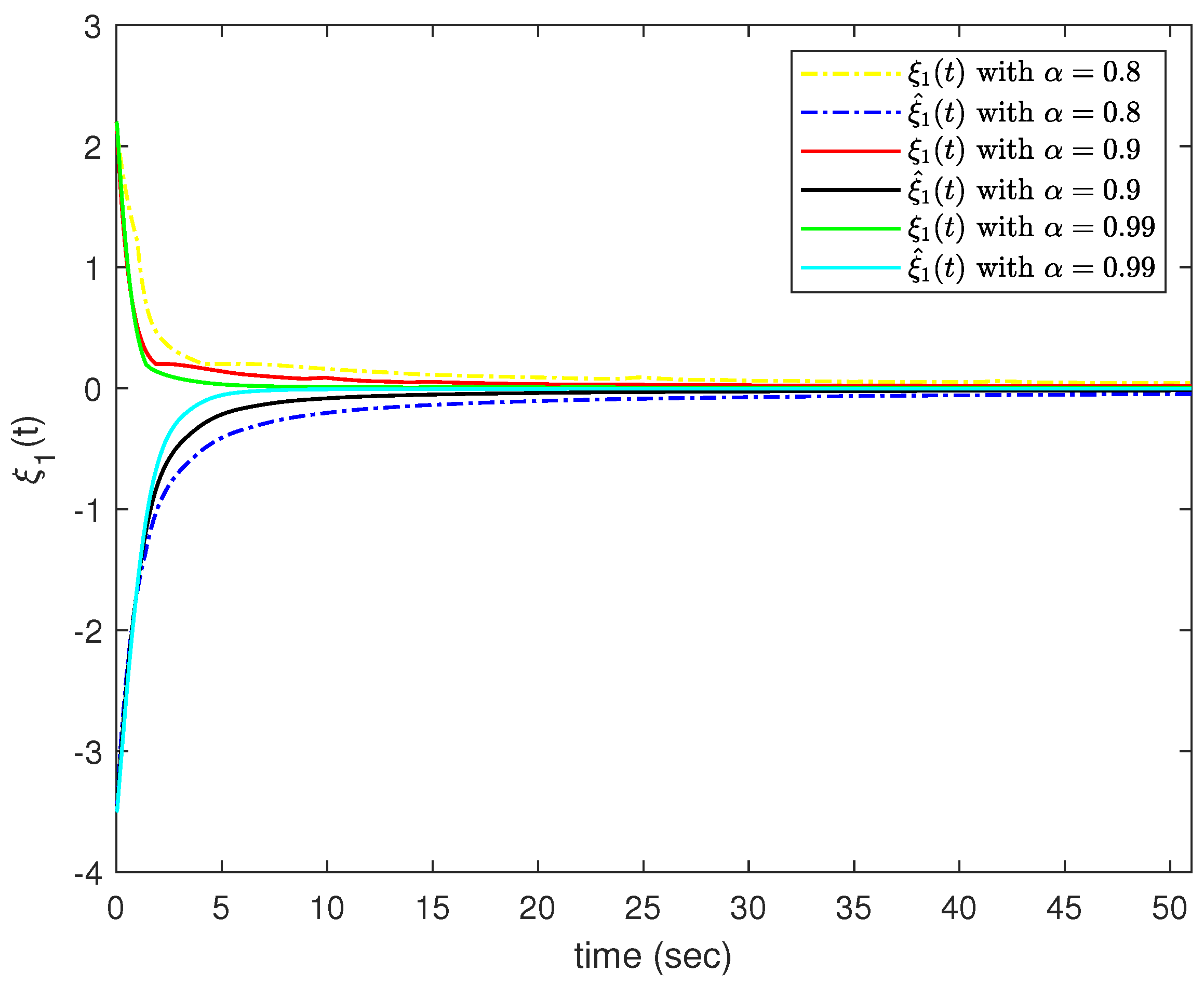
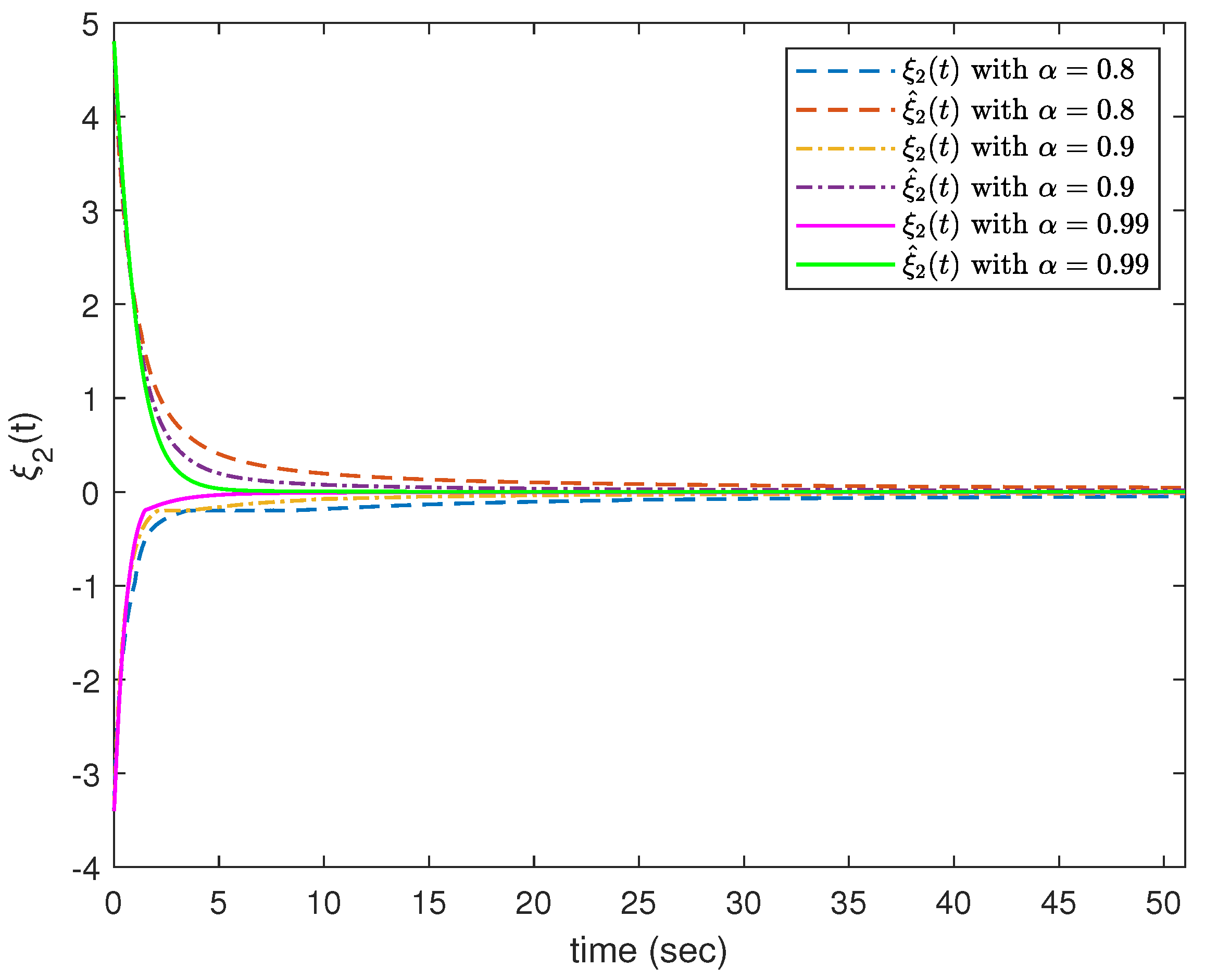
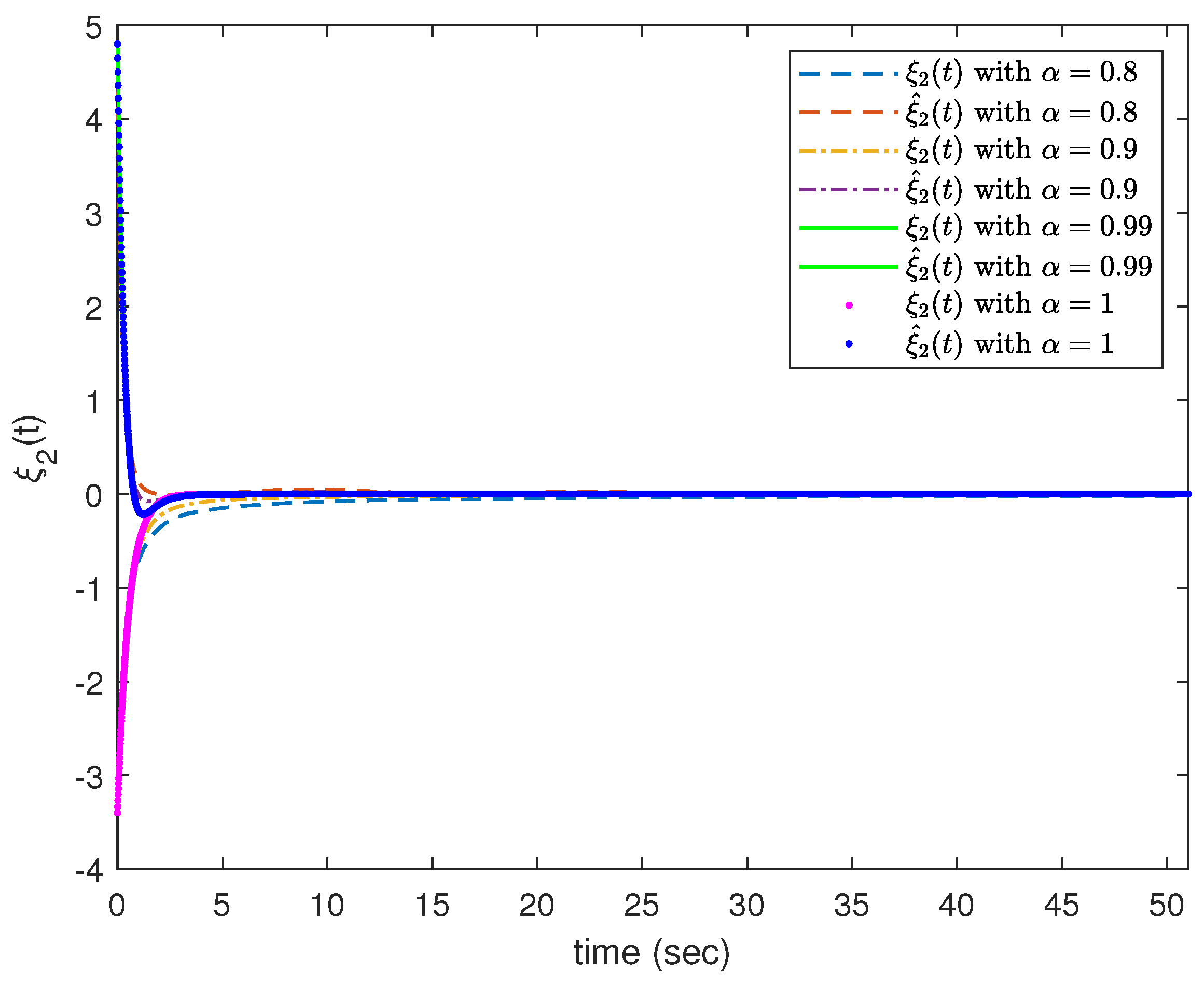
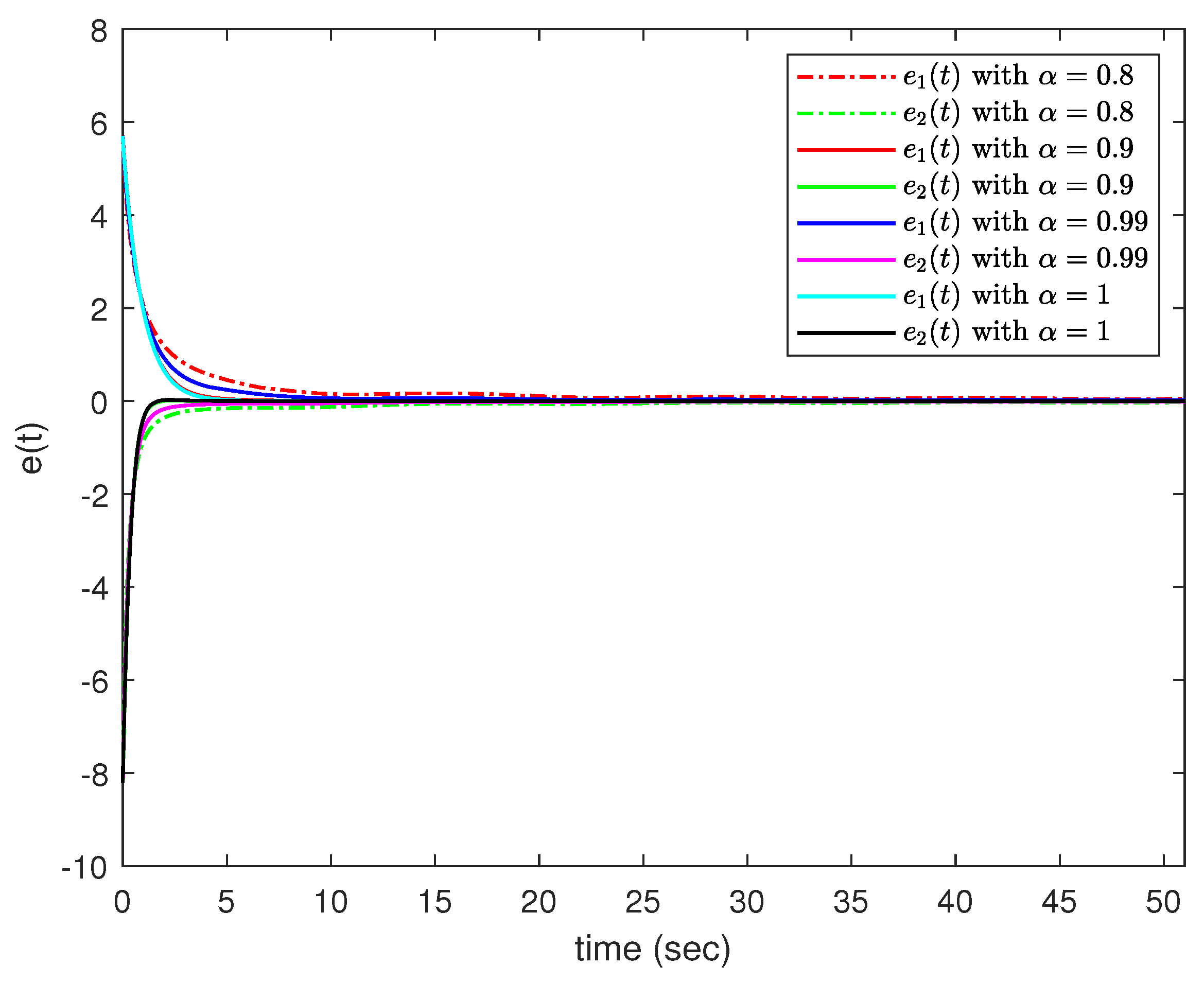
4. Examples and Simulations

Two numerical simulations are offered to illustrate the effectiveness of the proposed estimator algorithm.

Example 1.

Consider the following parameters of FOMNNs (3) as

$$a_{11}\left({\xi }_1\right)=\left\{\begin{array}{c}-0.5,|{\xi }_1|\le 1,\hfill \\ -0.6,|{\xi }_1|>1,\hfill \end{array}\right. a_{12}\left({\xi }_1\right)=\left\{\begin{array}{c}1,|{\xi }_1|\le 1,\hfill \\ 0.5,|{\xi }_1|>1,\hfill \end{array}\right.$$

$$a_{21}\left({\xi }_2\right)=\left\{\begin{array}{c}0.5,|{\xi }_2|\le 1,\hfill \\ -0.7,|{\xi }_2|>1,\hfill \end{array}\right. a_{22}\left({\xi }_2\right)=\left\{\begin{array}{c}-0.22,|{\xi }_2|\le 1,\hfill \\ -0.5,|{\xi }_2|>1,\hfill \end{array}\right.$$

$$b_{11}\left({\xi }_1\right)=\left\{\begin{array}{c}-0.6,|{\xi }_1|\le 1,\hfill \\ -0.5,|{\xi }_1|>1,\hfill \end{array}\right. b_{12}\left({\xi }_1\right)=\left\{\begin{array}{c}0.5,|{\xi }_1|\le 1,\hfill \\ 0.25,|{\xi }_1|>1,\hfill \end{array}\right.$$

$$b_{21}\left({\xi }_2\right)=\left\{\begin{array}{c}0.5,|{\xi }_2|\le 1,\hfill \\ -0.7,|{\xi }_2|>1,\hfill \end{array}\right. b_{22}\left({\xi }_2\right)=\left\{\begin{array}{c}-0.22,|{\xi }_2|\le 1,\hfill \\ -0.5,|{\xi }_2|>1,\hfill \end{array}\right.$$

$$e_{11}\left({\xi }_1\right)=\left\{\begin{array}{c}0.3,|{\xi }_1|\le 1,\hfill \\ -0.4,|{\xi }_1|>1,\hfill \end{array}\right. e_{12}\left({\xi }_1\right)=\left\{\begin{array}{c}0.5,|{\xi }_1|\le 1,\hfill \\ 0.13,|{\xi }_1|>1,\hfill \end{array}\right.$$

$$e_{21}\left({\xi }_2\right)=\left\{\begin{array}{c}0.2,|{\xi }_2|\le 1,\hfill \\ 1,|{\xi }_2|>1,\hfill \end{array}\right. e_{22}\left({\xi }_2\right)=\left\{\begin{array}{c}-0.7,|{\xi }_2|\le 1,\hfill \\ -0.3,|{\xi }_2|>1,\hfill \end{array}\right.$$

$$c_{11}\left({\xi }_1\right)=\left\{\begin{array}{c}0.1,|{\xi }_1|\le 1,\hfill \\ -0.3,|{\xi }_1|>1,\hfill \end{array}\right. c_{22}\left({\xi }_2\right)=\left\{\begin{array}{c}0.4,|{\xi }_2|\le 1,\hfill \\ 0.2,|{\xi }_2|>1,\hfill \end{array}\right.$$

$\mathcal{C}=\left[\begin{array}{cc}0.1& 0.3\\ 0.25& -0.4\end{array}\right],\mathcal{H}=\mathrm{diag}\left\{1,1\right\},\mathcal{N}=\left[0.30.4;0.40.3\right]$. We choose the distribute delay $\mathfrak{d}\left(t\right)=0.05+0.3\left|cos\right(t\left)\right|$ with $\mathfrak{d}=0.35$.

Assume that the occurring probability of the time-varying delays $\varrho \left(t\right),\mathfrak{d}\left(t\right)$ satisfy $\overline{\gamma }=\mathbb{E}\left\{\gamma \left(t\right)\right\}=0.7,\overline{\delta }=\mathbb{E}\left\{\delta \left(t\right)\right\}=0.9$. Set the activation function as

$$f\left(\xi \left(t\right)\right)=\left[\begin{array}{c}-0.4{\xi }_1\left(t\right)+\tanh \left(0.2{\xi }_1\left(t\right)\right)+0.3{\xi }_2\left(t\right)\\ -0.2{\xi }_2\left(t\right)+\tanh \left(0.3{\xi }_2\left(t\right)\right)\end{array}\right],$$

then,

$${\overrightarrow{F}}_1=\left[\begin{array}{cc}-0.4& 0.3\\ 0& -0.2\end{array}\right],{\overrightarrow{F}}_2=\left[\begin{array}{cc}-0.2& 0.3\\ 0& 0.1\end{array}\right]$$

By employing the Matlab LMI Toolbox for the resolution of the LMIs (32), the following feasible solutions can be obtained:

$$\begin{array}{c}\hfill \overrightarrow{\mathcal{W}}=\left[\begin{array}{cc}0.0374& 0.0037\\ 0.0037& 0.0332\end{array}\right],\mathcal{K}=\left[\begin{array}{cc}-0.0688& -0.2333\\ -0.2146& 0.2782\end{array}\right],\end{array}$$

and ${\kappa }_1=1.1590,{\kappa }_2=0.6043,{\kappa }_3=0.2919,\mathfrak{r}=0.2031,\mathfrak{s}=0.3796,\mathfrak{u}=0.3448,\mathfrak{t}=0.3348$.

In this simulation, the fractional-order estimation system subject to sensor saturation is considered. According to the above parameters, all the simulation results with various orders are present in Figure 1, Figure 2 and Figure 3. Figure 1 and Figure 2 illustrate the state and corresponding estimates of neurons ${\xi }_1\left(t\right),{\xi }_2\left(t\right)$, respectively. Figure 3 shows the errors with different orders ($\alpha =0.8,0.9,0.99$) between ${\xi }_i\left(t\right)$ and ${\hat{\xi }}_i\left(t\right)$. Therefore, the validity of the proposed theoretical results is verified in this numerical simulation.

Example 2.

In what follows, the following delayed FOMNNs model subject to sensor saturations is considered:

$$\begin{array}{c}\hfill D^{\alpha }\xi \left(t\right)=-\mathcal{C}\left(t\right)\xi \left(t\right)+\mathcal{A}\left(t\right)g\left(\xi \left(t\right)\right)+\mathcal{B}\left(t\right)f\left(\xi (t-\varrho \left(t\right))\right),\end{array}$$

(41)

In this example, the following parameters are chosen:

$$a_{11}\left({\xi }_1\right)=\left\{\begin{array}{c}-1.5,|{\xi }_1|\le 1,\hfill \\ -1,|{\xi }_1|>1,\hfill \end{array}\right. a_{12}\left({\xi }_1\right)=\left\{\begin{array}{c}-0.2,|{\xi }_1|\le 1,\hfill \\ 0.6,|{\xi }_1|>1,\hfill \end{array}\right.$$

$$a_{21}\left({\xi }_2\right)=\left\{\begin{array}{c}0.3,|{\xi }_2|\le 1,\hfill \\ 0.1,|{\xi }_2|>1,\hfill \end{array}\right. a_{22}\left({\xi }_2\right)=\left\{\begin{array}{c}-0.2,|{\xi }_2|\le 1,\hfill \\ -0.6,|{\xi }_2|>1,\hfill \end{array}\right.$$

$$b_{11}\left({\xi }_1\right)=\left\{\begin{array}{c}-1,|{\xi }_1|\le 1,\hfill \\ -0.5,|{\xi }_1|>1,\hfill \end{array}\right. b_{12}\left({\xi }_1\right)=\left\{\begin{array}{c}-0.35,|{\xi }_1|\le 1,\hfill \\ 0.65,|{\xi }_1|>1,\hfill \end{array}\right.$$

$$b_{21}\left({\xi }_2\right)=\left\{\begin{array}{c}-0.3,|{\xi }_2|\le 1,\hfill \\ 0.5,|{\xi }_2|>1,\hfill \end{array}\right. b_{22}\left({\xi }_2\right)=\left\{\begin{array}{c}-0.5,|{\xi }_2|\le 1,\hfill \\ -0.75,|{\xi }_2|>1,\hfill \end{array}\right.$$

$$c_{11}\left({\xi }_1\right)=\left\{\begin{array}{c}1.5,|{\xi }_1|\le 1,\hfill \\ 1.3,|{\xi }_1|>1,\hfill \end{array}\right. c_{22}\left({\xi }_2\right)=\left\{\begin{array}{c}1.62,|{\xi }_2|\le 1,\hfill \\ 1.2,|{\xi }_2|>1,\hfill \end{array}\right.$$

$\mathcal{H}=\left[11;11\right],\mathcal{N}=\left[0.2-0.2;-0.20.2\right],{\mathcal{G}}_1=\mathrm{diag}\left\{0.7,0.85\right\},\mathcal{G}=\mathrm{diag}\left\{0.4,0.5\right\}$.

By means of the Matlab Tool to solve the inequalities (32), we have the following feasible solutions:

$$\begin{array}{c}\hfill {\mathcal{W}}_2=\left[\begin{array}{cc}2.9114& 3.2613\\ 3.2613& 8.9590\end{array}\right],{\mathcal{K}}^{\prime }=\left[\begin{array}{cc}-0.7373& -0.4956\\ 0.3563& 1.6337\end{array}\right],\end{array}$$

and ${\kappa }_1=0.201,{\kappa }_2=0.1576,{\kappa }_3=0.3506,\overrightarrow{\mathfrak{u}}=0.13,\overrightarrow{\mathfrak{r}}=0.3513$.

In this simulation, Figure 4, Figure 5 and Figure 6 show all the simulation results with different orders. Under sensor saturation, Figure 6 depicts the estimation error with mixed time-varying delays. Figure 4 and Figure 5 show the trajectories of neurons ${\xi }_1\left(t\right),{\xi }_2\left(t\right)$ and the corresponding estimation, respectively. Under the different orders ($\alpha =0.8,0.9,0.99,1$), it is clear that the estimation errors converge to zeros finally, which verifies the effectiveness of the designed estimator scheme. In addition, from

Table 1. Maximal allowable delay ${\varrho }_{max}$ with different $\overline{\varrho }(\alpha =0.9)$.

Method	$\overline{\mathit{\varrho }}=0.2$	$\overline{\mathit{\varrho }}=0.5$	$\overline{\mathit{\varrho }}=0.8$	NDVs
[10]	3.1802	2.8591	2.1934	76
[38]	6.541	6.0684	4.9716	132
Theorem 1	6.7168	5.9754	5.0197	188

, the maximal allowable delay ${\varrho }_{max}$ and the number of decision variables (NDVs) can be obtained. This indicates that the allowable upper bound is superior to the previous methods. In this paper, we introduce double integrals and triple integrals, which require more decision variables than the methods discussed in [38]. The method proposed in this paper is less conservative.

5. Conclusions

This paper investigates the nonfragile SE for FOMNNs with ROTDs subject to sensor saturation. Considering the load on network bandwidth, a logarithmic quantizer is introduced to design the fraction-order estimator. Based on a novel Caputo–Wirtinger integral inequalities, a lower conversation criterion is established to guarantee the augmented system is stochastically asymptotically stable. In the end, two numerical simulations are shown to illustrate the validity of the proposed estimation scheme. Furthermore, it is possible to apply the proposed method and scheme to fractional-order uncertain systems or complex-valued neural networks with an event-triggered scheme [52,53,54].

References

1. Oldham, K.; Spanier, J. The Fractional Calculus Theory and Applications of Differentiation and Integration to Arbitrary Order; Elsevier: Amsterdam, The Netherlands, 1974. [Google Scholar]
2. Alarifi, N.M.; Ibrahim, R.W. Specific Classes of Analytic Functions Communicated with a Q-Differential Operator Including a Generalized Hypergeometic Function. Fractal Fract. 2022, 6, 545. [Google Scholar] [CrossRef]
3. Hilfer, R. Applications of Fractional Calculus in Physics; World Scientific: Singapore, 2000. [Google Scholar]
4. El-Nabulsi, R.A.; Torres, D.F. Fractional actionlike variational problems. J. Math. Phys. 2008, 49, 053521. [Google Scholar] [CrossRef]
5. Podlubny, I. Fractional-order systems and PI/sup/spl lambda//D/sup/spl mu//-controllers. IEEE Trans. Autom. Control 1999, 44, 208–214. [Google Scholar] [CrossRef]
6. Miller, K.S.; Ross, B. An Introduction to the Fractional Calculus and Fractional Differential Equations; Wiley: Hoboken, NJ, USA, 1993. [Google Scholar]
7. Cheng, Y.; Xu, W.; Jia, H.; Zhong, S. Stability analysis of fractional-order neural networks with time-varying delay utilizing free-matrix-based integral inequalities. J. Frankl. Inst. 2023, 360, 10815–10835. [Google Scholar] [CrossRef]
8. Li, H.l.; Jiang, H.; Cao, J. Global synchronization of fractional-order quaternion-valued neural networks with leakage and discrete delays. Neurocomputing 2019, 385, 211–219. [Google Scholar] [CrossRef]
9. Parvizian, M.; Khandani, K.; Majd, V.J. An H non-fragile observer-based adaptive sliding mode controller design for uncertain fractional-order nonlinear systems with time delay and input nonlinearity. Asian J. Control 2021, 23, 423–431. [Google Scholar] [CrossRef]
10. Chen, L.; Li, T.; Wu, R.; Chen, Y.; Liu, Z. Non-fragile control for a class of fractional-order uncertain linear systems with time-delay. IET Control Theory Appl. 2020, 14, 1575–1589. [Google Scholar] [CrossRef]
11. Qiu, H.; Shen, J.; Cao, J.; Liu, H. L-Gain of Fractional-Order Positive Systems with Mixed Time-Varying Delays. IEEE Trans. Circuits Syst. Regul. Pap. 2024, 71, 828–837. [Google Scholar] [CrossRef]
12. Nassajian, G.; Balochian, S. Multi-model estimation using neural network and fault detection in unknown time continuous fractional order nonlinear systems. Trans. Inst. Meas. Control 2021, 43, 497–509. [Google Scholar] [CrossRef]
13. Tong, P.; Xu, H.; Sun, Y.; Wang, Y.; Peng, J.; Liao, C.; Wang, W.; Li, Q. Lightweight and highly robust memristor-based hybrid neural networks for electroencephalogram signal processing. Chin. Phys. B 2023, 32, 078505. [Google Scholar] [CrossRef]
14. Zhang, X.; Jiang, D.; Nkapkop, J.D.D.; Njitacke, Z.T.; Ahmad, M.; Zhu, L.; Tsafack, N. A memristive autapse-synapse neural network: Application to image encryption. Phys. Scr. 2023, 98, 035222. [Google Scholar] [CrossRef]
15. Li, J.; Dong, H.; Wang, Z.; Bu, X. Partial-Neurons-Based Passivity-Guaranteed State Estimation for Neural Networks with Randomly Occurring Time Delays. IEEE Trans. Neural Netw. Learn. Syst. 2020, 31, 3747–3753. [Google Scholar] [CrossRef]
16. Xiao, J.; Li, Y.; Zhong, S.; Xu, F. Extended dissipative state estimation for memristive neural networks with time-varying delay. ISA Trans. 2016, 64, 113–128. [Google Scholar] [CrossRef]
17. Nagamani, G.; Karnan, A.; Soundararajan, G. Delay-Dependent and Independent State Estimation for BAM Cellular Neural Networks with Multi-Proportional Delays. Circuits Syst. Signal Process. 2021, 40, 3179–3203. [Google Scholar] [CrossRef]
18. Tan, Y.; Xiong, M.; Zhang, B.; Fei, S. Adaptive Event-Triggered Nonfragile State Estimation for Fractional-Order Complex Networked Systems with Cyber Attacks. IEEE Trans. Syst. Man Cybern. Syst. 2022, 52, 2121–2133. [Google Scholar] [CrossRef]
19. Li, Q.; Wang, Z.; Sheng, W.; Alsaadi, F.E.; Alsaadi, F.E. Dynamic event-triggered mechanism for H non-fragile state estimation of complex networks under randomly occurring sensor saturations. Inf. Sci. 2020, 509, 304–316. [Google Scholar] [CrossRef]
20. Chua, L. Memristor-the missing circuit element. IEEE Trans. Circuit Theory 1971, 18, 507–519. [Google Scholar] [CrossRef]
21. Strukov, D.B.; Snider, G.S.; Stewart, D.R.; Williams, R.S. The missing memristor found. Nature 2008, 453, 80–83. [Google Scholar] [CrossRef]
22. Guo, T.; Sun, B.; Ranjan, S.; Jiao, Y.; Wei, L.; Zhou, Y.N.; Wu, Y.A. From Memristive Materials to Neural Networks. ACS Appl. Mater. Interfaces 2020, 12, 54243–54265. [Google Scholar] [CrossRef]
23. Tsafack, N.; Iliyasu, A.M.; De Dieu, N.J.; Zeric, N.T.; Kengne, J.; Abd-El-Atty, B.; Belazi, A.; Abd EL-Latif, A.A. A memristive RLC oscillator dynamics applied to image encryption. J. Inf. Secur. Appl. 2021, 61, 102944. [Google Scholar] [CrossRef]
24. Duan, S.; Hu, X.; Dong, Z.; Wang, L.; Mazumder, P. Memristor-Based Cellular Nonlinear/Neural Network: Design, Analysis, and Applications. IEEE Trans. Neural Netw. Learn. Syst. 2015, 26, 1202–1213. [Google Scholar] [CrossRef]
25. Popa, C.A. Mittag-Leffler stability and synchronization of neutral-type fractional-order neural networks with leakage delay and mixed delays. J. Frankl. Inst. 2023, 360, 327–355. [Google Scholar] [CrossRef]
26. Jia, J.; Wang, F.; Zeng, Z. Global stabilization of fractional-order memristor-based neural networks with incommensurate orders and multiple time-varying delays: A positive-system-based approach. Nonlinear Dyn. 2021, 104, 2303–2329. [Google Scholar] [CrossRef]
27. Hong, D.T.; Sau, N.H.; Thuan, M.V. New Criteria for Dissipativity Analysis of Fractional-Order Static Neural Networks. Circuits Syst. Signal Process. 2022, 41, 2221–2243. [Google Scholar] [CrossRef]
28. Bao, H.; Cao, J.; Kurths, J. State estimation of fractional-order delayed memristive neural networks. Nonlinear Dyn. 2018, 94, 1215–1225. [Google Scholar] [CrossRef]
29. Nagamani, G.; Shafiya, M.; Soundararajan, G. An LMI based state estimation for fractional-order memristive neural networks with leakage and time delays. Neural Process. Lett. 2020, 52, 2089–2108. [Google Scholar] [CrossRef]
30. Li, R.; Gao, X.; Cao, J. Quasi-state estimation and quasi-synchronization control of quaternion-valued fractional-order fuzzy memristive neural networks: Vector ordering approach. Appl. Math. Comput. 2019, 362, 124572. [Google Scholar] [CrossRef]
31. Dorato, P. Non-fragile controller design: An overview. In Proceedings of the 1998 American Control Conference, ACC 1998, Philadelphia, PA, USA, 24–26 June 1998; Volume 5, pp. 2829–2831. [Google Scholar]
32. Zha, L.; Fang, J.-A.; Liu, J.; Tian, E. Event-triggered non-fragile state estimation for delayed neural networks with randomly occurring sensor nonlinearity. Neurocomputing 2018, 273, 1–8. [Google Scholar] [CrossRef]
33. Shao, X.; Lyu, M.; Zhang, J. Nonfragile estimator design for fractional-order neural networks under event-triggered mechanism. Discret. Dyn. Nat. Soc. 2021, 2021, 6695353. [Google Scholar] [CrossRef]
34. Bao, H.; Park, J.H.; Cao, J. Non-fragile state estimation for fractional-order delayed memristive BAM neural networks. Neural Netw. 2019, 119, 190–199. [Google Scholar] [CrossRef]
35. Liu, J.; Xia, J.; Cao, J.; Tian, E. Quantized state estimation for neural networks with cyber attacks and hybrid triggered communication scheme. Neurocomputing 2018, 291, 35–49. [Google Scholar] [CrossRef]
36. Zhang, H.; Ye, R.; Liu, S.; Cao, J.; Alsaedi, A.; Li, X. LMI-based approach to stability analysis for fractional-order neural networks with discrete and distributed delays. Int. J. Syst. Sci. 2018, 49, 537–545. [Google Scholar] [CrossRef]
37. Shao, X.G.; Zhang, J.; Lu, Y.J. Event-based nonfragile state estimation for memristive recurrent neural networks with stochastic cyber-attacks and sensor saturations. Chin. Phys. B 2024. [Google Scholar] [CrossRef]
38. Chen, S.; Song, Q.; Zhao, Z.; Liu, Y.; Alsaadi, F.E. Global asymptotic stability of fractional-order complex-valued neural networks with probabilistic time-varying delays. Neurocomputing 2021, 450, 311–318. [Google Scholar] [CrossRef]
39. Ali, M.S.; Hymavathi, M.; Saroha, S.; Moorthy, R.K. Global asymptotic stability of neutral type fractional-order memristor-based neural networks with leakage term, discrete and distributed delays. Math. Methods Appl. Sci. 2021, 44, 5953–5973. [Google Scholar]
40. Podlubny, I. Fractional Differential Equations: An Introduction to Fractional Derivatives, Fractional Differential Equations, to Methods of Their Solution and Some of Their Applications; Elsevier: Amsterdam, The Netherlands, 1998. [Google Scholar]
41. Aubin, J.P.; Frankowska, H. Set-Valued Analysis; Springer: Berlin/Heidelberg, Germany, 2009. [Google Scholar]
42. Zhang, R.; Zeng, D.; Zhong, S.; Yu, Y. Event-triggered sampling control for stability and stabilization of memristive neural networks with communication delays. Appl. Math. Comput. 2017, 310, 57–74. [Google Scholar] [CrossRef]
43. Cheng, J.; Liang, L.; Park, J.H.; Yan, H.; Li, K. A Dynamic Event-Triggered Approach to State Estimation for Switched Memristive Neural Networks with Nonhomogeneous Sojourn Probabilities. IEEE Trans. Circuits Syst. Regul. Pap. 2021, 68, 4924–4934. [Google Scholar] [CrossRef]
44. Guo, M.; Zhu, S.; Liu, X. Observer-based state estimation for memristive neural networks with time-varying delay. Knowl.-Based Syst. 2022, 246, 108707. [Google Scholar]
45. Wang, Z.; Ding, S.; Huang, Z.; Zhang, H. Exponential Stability and Stabilization of Delayed Memristive Neural Networks Based on Quadratic Convex Combination Method. IEEE Trans. Neural Netw. Learn. Syst. 2016, 27, 2337–2350. [Google Scholar] [CrossRef]
46. Geng, H.; Wang, Z.; Hu, J.; Alsaadi, F.E.; Cheng, Y. Outlier-resistant sequential filtering fusion for cyber-physical systems with quantized measurements under denial-of-service attacks. Inf. Sci. 2023, 628, 488–503. [Google Scholar] [CrossRef]
47. Fu, M.; Xie, L. The sector bound approach to quantized feedback control. IEEE Trans. Autom. Control 2005, 50, 1698–1711. [Google Scholar]
48. Cao, Y.Y.; Lin, Z.; Chen, B.M. An output feedback/spl Hscr//sub/spl infin//controller design for linear systems subject to sensor nonlinearities. IEEE Trans. Circuits Syst. Fundam. Theory Appl. 2003, 50, 914–921. [Google Scholar]
49. Zhang, S.; Yu, Y.; Yu, J. LMI conditions for global stability of fractional-order neural networks. IEEE Trans. Neural Netw. Learn. Syst. 2016, 28, 2423–2433. [Google Scholar] [CrossRef]
50. Yang, X.; Wu, X.; Song, Q. Caputo–Wirtinger integral inequality and its application to stability analysis of fractional-order systems with mixed time-varying delays. Appl. Math. Comput. 2024, 460, 128303. [Google Scholar] [CrossRef]
51. Gu, K.; Chen, J.; Kharitonov, V.L. Stability of Time-Delay Systems; Springer: Berlin/Heidelberg, Germany, 2003. [Google Scholar]
52. Jiang, Z.; Huang, F.; Shao, H.; Cai, S.; Lu, X.; Jiang, S. Time-varying finite-time synchronization analysis of attack-induced uncertain neural networks. Chaos Solitons Fractals 2023, 175, 113954. [Google Scholar] [CrossRef]
53. Xu, B.; Li, B. Dynamic Event-Triggered Consensus for Fractional-Order Multi-Agent Systems without Intergroup Balance Condition. Fractal Fract. 2023, 7, 268. [Google Scholar] [CrossRef]
54. Hymavathi, M.; Muhiuddin, G.; Syed Ali, M.; Al-Amri, J.F.; Gunasekaran, N.; Vadivel, R. Global Exponential Stability of Fractional Order Complex-Valued Neural Networks with Leakage Delay and Mixed Time Varying Delays. Fractal Fract. 2022, 6, 140. [Google Scholar] [CrossRef]
Figure 1. Responses of ξ i ( t ) and ξ ^ i ( t ) with α = 0.8 , 0.9 , 0.99 .
Fractalfract 08 00343 g001
Figure 2. Responses of ξ i ( t ) and ξ ^ i ( t ) with α = 0.8 , 0.9 , 0.99 .
Fractalfract 08 00343 g002
Figure 3. Estimation errors e i ( t ) under sensor saturation.
Fractalfract 08 00343 g003
Figure 4. Trajectories of ξ 1 ( t ) and ξ ^ 1 ( t ) with α = 0.8 , 0.9 , 0.99 , 1 .
Fractalfract 08 00343 g004
Figure 5. Trajectories of ξ 2 ( t ) and ξ ^ 2 ( t ) with α = 0.8 , 0.9 , 0.99 , 1 .
Fractalfract 08 00343 g005
Figure 6. The estimation errors e i ( t ) under sensor saturation.
Fractalfract 08 00343 g006