Event-Triggered Adaptive Neural Network Control for State-Constrained Pure-Feedback Fractional-Order Nonlinear Systems with Input Delay and Saturation

Abstract

In this research, the adaptive event-triggered neural network controller design problem is investigated for a class of state-constrained pure-feedback fractional-order nonlinear systems (FONSs) with external disturbances, unknown actuator saturation, and input delay. An auxiliary compensation function based on the integral function of the input signal is presented to handle input delay. The barrier Lyapunov function (BLF) is utilized to deal with state constraints, and the event-triggered strategy is applied to overcome the communication burden from the limited communication resources. By the utilization of a backstepping scheme and radial basis function neural network, an adaptive event-triggered neural state-feedback stabilization controller is constructed, in which the fractional-order dynamic surface filters are employed to reduce the computational burden from the recursive procedure. It is proven that with the fractional-order Lyapunov analysis, all the solutions of the closed-loop system are bounded, and the tracking error can converge to a small interval around the zero, while the state constraint is satisfied and the Zeno behavior can be strictly ruled out. Two examples are finally given to show the effectiveness of the proposed control strategy.

1. Introduction

Fractional-order dynamical behavior has been found in many practical systems [1,2], which can achieve more precise representations for complex physical systems with infinite memory and genetic characteristics. Based on this fact, fractional-order nonlinear systems (FONSs) offer an effective way to model the physical system [3,4], which can be applied in lots of areas [5,6,7,8,9]. Moreover, the nonlinear controller design problem for FONSs has received a lot of attention, and many controller design approaches have been investigated [10,11,12,13,14,15], in which the approximation performance of fuzzy logic systems (FLSs) or neural networks (NNs) can be used to deal with nonlinear unknown function in FONSs to achieve stability. In [16], an adaptive controller by using the property of NNs is considered for FONSs with actuator fault. In [17], a fuzzy controller is designed for nonstrict-feedback FONSs. In [18], a distributed backstepping control for nonaffine FONSs with unknown dynamics is presented, and the stability is accomplished. For fractional-order tumor systems with chemotherapy in [19], a finite-time fuzzy controller is developed under Lyapunov theory. It is worth noting that the influence of full state constraints on FONSs has not been taken into account in the above-mentioned literature and achievements.

System constraints often appear in many real industrial processes and practical systems unavoidably, which is the main factor limiting system performance, leading to instability of the system. To settle such system constraints, a crucial problem for FONSs, the barrier Lyapunov function (BLF) has become one of the most powerful tools to prevent transgression of state constraints, and many constraint control strategies have been designed [20,21,22,23]. In [21], an observer-based adaptive NN controller is proposed for nonstrict-feedback FONSs with an output constraint, where the tracking error satisfying constraints can be guaranteed. In [22], a distributed adaptive controller is designed for multiple FONSs with constraints, and the BLF is applied to restrict the output in the preset range. In [23], an adaptive dynamic surface controller for FONSs with asymmetric state constraints is designed by using an asymmetric BLF. Nevertheless, it is important that the characteristics of the control input signal should not be ignored.

It is inevitable that the input saturation is the important non-smooth nonlinearity in many practical engineering systems due to the physical characteristics of the actuator. Once the control input exceeds the upper, it may not work properly and can unquestionably limit its control performance. Then, it is important to take the effect of actuator saturation into consideration during the process of the design and analysis of FONSs [24,25,26]. The author in [24] introduced the fractional-order finite-time adaptive fault-tolerant control for an unmanned aerial vehicle with the saturated actuator, wherein the input saturation function is approximated using the smooth function. In [26], the flexible spacecraft attitude adjustment with input torque saturation is considered, and a fractional-order multi-objective controller is presented. For a vertical takeoff vertical landing reusable launch vehicle subjected to input saturation constraints, a fractional-order fixed-time sliding mode controller with state observer is designed in [25]. However, in the above-mentioned research for FONSs, the issue of the widely existing input delay is ignored.

In the control process for real engineering applications, it takes time to send signals to actuators causing the input delays of the system, and is the major factor in deteriorating the system performance. To deal with the input delay, many effective methods are developed for FONSs in [27,28,29,30]. In [27], a feedback controller for a fractional-order system under input delay is designed by using the Smith predictor. In [28], an augmented adaptive controller based on the function approximation technique is developed for FONSs with input delay. In [29], a command-filter-based adaptive controller for FONSs with input delay is designed by using the fractional integral. In [30], an adaptive NN control method for FONSs with input delay is developed by using the auxiliary system. However, no results about the adaptive control strategy of state-constrained FONSs with input delay and actuator saturation can be found.

Motivated by the above-mentioned discussions, the adaptive neural network event-triggered control (ETC) for state-constrained pure-feedback FONSs with input delay and unknown actuator saturation will be investigated. The highlighted innovations of this article are as follows:

(1)

Compared with fractional-order controller results [31,32,33], the full-state constraints, input delay, and unknown actuator saturation are investigated simultaneously in this article, and the BLFs and neural network are introduced into the design process of the backstepping technique, which can ensure that state convergence without contravening state constraints can be guaranteed, and the boundedness of all the closed-loop system signals can be accomplished.

(2)

Compared with controller designed for FONSs subject to input delay in [27,28,29,30,34], the event-triggered mechanism is designed to reduce the communications constraints of network resources, and the fractional-order dynamic surface filter is presented to remove the explosion of differentiation from the recursive procedure, which effectively makes the proposed controller more suitable for practical engineering.

The rest of this paper is organized as follows. The preliminaries and problem formulation are presented in Section 2 and Section 3, respectively. Then, the proposed adaptive control scheme for FONSs with input delay is provided in Section 4. The simulation studies are given in Section 5 to show the effectiveness. Section 6 concludes this paper.

2. Preliminaries

The $\alpha$th Caputo fractional derivative of $f\left(t\right)$ is defined as [35,36]:

$$D_{t_0}^{\alpha }f\left(t\right)=\frac{1}{\Gamma \left(n-\alpha \right)}{\int }_{t_0}^t\frac{f^{\left(n\right)}\left(t\right)}{{\left(t-\tau \right)}^{\alpha +1-n}}d\tau$$

where $n-1<\alpha <n,n$ is the positive integer, $\Gamma \left(\alpha \right)={\int }_0^{\infty }{e}^{-t}{t}^{\alpha -1}dt$ is the Euler Gamma function, and $D_{t_0}^{\alpha }$ can be abbreviated as $D^{\alpha }$, when $t_0=0$.

Lemma 1

([35]). If $\varphi \in \left(\frac{\pi \alpha }{2},\pi \alpha \right)$, then $\exists \beta >0$, such that

$$\left|E_{\alpha ,\gamma }\left(\zeta \right)\right|\le \frac{\beta }{1+\left|\zeta \right|},\gamma \le \left|arg\left(\zeta \right)\right|\le \pi ,\left|\zeta \right|\ge 0$$

where $E_{\alpha ,\gamma }\left(\zeta \right)={\displaystyle \sum _{k=0}^{\infty }}\frac{{\zeta }^k}{\Gamma \left(\alpha k-\gamma \right)}$ is the one-parameter Mittag–Leffler function, ζ is a complex number, and $\alpha ,\gamma >0$. Note that $E_{\alpha ,1}\left(\zeta \right)=E_{\alpha }\left(\zeta \right)$ and $E_{1,1}\left(\zeta \right)=e^{\zeta }$.

Lemma 2

([37,38]). Let $x\left(t\right)\in {\mathbb{R}}^n$ be a differentiable function. Then, $D^{\alpha }\left(x^{\mathrm{T}}\left(t\right)Px\left(t\right)\right)\le 2x^{\mathrm{T}}\left(t\right)P{D}^{\alpha }\left(x\left(t\right)\right)$ holds for $\forall t\ge t_0$, where $P=P^{\mathrm{T}}>0$.

Lemma 3

([39]). Let $h_1\left(·\right),h_2\left(·\right)\in \mathbb{R}$ be smooth functions. If $h_1\left(h_2\right)$ is convex (i.e., ${\partial }^2{h}_1\left(h_2\right)/\phantom{{\partial }^2{h}_1\left(h_2\right)\partial h_2^2}\partial h_2^2\ge 0$), then, $D^{\alpha }{h}_1\left(h_2\right)\le \partial h_1\left(h_2\right)/\phantom{D^{\alpha }{h}_1\left(h_2\right)\le \partial h_1\left(h_2\right)\partial h_2}\partial h_2·D^{\alpha }{h}_2$ for $\forall t\ge 0$.

Lemma 4

([40]). Let the function $V\left(t\right):{\mathbb{R}}^{+}\to \mathbb{R}$ satisfying $D^{\alpha }V\left(t\right)+\eta V\left(t\right)\le \mu$, where $\eta >0$, and $\mu \ge 0$. Then, $V\left(t\right)\le V\left(0\right)E_{\left(\alpha ,1\right)}\left(-\eta t^{\alpha }\right)+\frac{\mu \vartheta }{\eta }$, where $\vartheta =max\left\{1,\beta \right\}$ and β is defined in Lemma 1.

Lemma 5

([41,42]). For $\forall k_{b_0}>0$, the following inequality holds

$$ln\frac{k_{b_0}^2}{k_{b_0}^2-{\varsigma }^2\left(t\right)}\le \frac{{\varsigma }^2\left(t\right)}{k_{b_0}^2-{\varsigma }^2\left(t\right)}$$

if $\left|\varsigma \left(t\right)\right|\le k_{b_0}$.

Lemma 6

([43]). For $\forall {\epsilon }^{*}>0$ and $s\in \mathbb{R}$, it holds $\left|s\right|-stanh\left(\frac{s}{{\epsilon }^{*}}\right)\le 0.2785{\epsilon }^{*}$.

Lemma 7

([44]). Let $h\left(x\right)$ be a continuous function. For $\forall \epsilon >0$, there is a radial basis function NN (RBFNN) $W^{\mathrm{T}}\Psi \left(x\right)$ satisfying $h\left(x\right)=W^{\mathrm{T}}\Psi \left(x\right)+\epsilon$, where $W={\left(\begin{array}{cccc}{w}_1& w_2& \cdots & w_N\end{array}\right)}^{\mathrm{T}}$, ε is an approximation error. $\Psi \left(x\right)={\left(\begin{array}{cccc}{\psi }_1\left(x\right)& {\psi }_2\left(x\right)& \cdots & {\psi }_N\left(x\right)\end{array}\right)}^{\mathrm{T}}/\phantom{{\left(\begin{array}{cccc}{\psi }_1\left(x\right)& {\psi }_2\left(x\right)& \cdots & {\psi }_N\left(x\right)\end{array}\right)}^{\mathrm{T}}{\sum }_{i=1}^N{\psi }_i\left(x\right)}{\sum }_{i=1}^N{\psi }_i\left(x\right)\in {\mathbb{R}}^N$, $N>1$ denotes node number, ${\psi }_i\left(x\right)=exp\left(-{\left(x-l_i\right)}^{\mathrm{T}}\left(x-l_i\right)/\phantom{-{\left(x-l_i\right)}^{\mathrm{T}}\left(x-l_i\right){\chi }_i^{\mathrm{T}}{\chi }_i}{\chi }_i^{\mathrm{T}}{\chi }_i\right)$, $l_i={\left(\begin{array}{cccc}{l}_{i1}& l_{i2}& \cdots & l_{in}\end{array}\right)}^{\mathrm{T}}$, and ${\chi }_i={\left(\begin{array}{cccc}{\chi }_{i1}& {\chi }_{i2}& \cdots & {\chi }_{in}\end{array}\right)}^{\mathrm{T}}$.

3. System Descriptions and Problem Formulation

A class of pure-feedback FONSs with input delay and unknown actuator saturation is considered as follows:

$$\left\{\begin{array}{c}{D}^{\alpha }{x}_i=f_i\left({\overline{x}}_i,x_{i+1}\right)+d_i\left(t\right),i=1,2,\dots ,n-1\hfill \\ D^{\alpha }{x}_n=f_n\left({\overline{x}}_n\right)+u\left(\nu \left(t-\tau \right)\right)+d_n\left(t\right)\hfill \\ y=x_1\hfill \end{array}\right.$$

(1)

where $\alpha \in \left(0,1\right]$, ${\overline{x}}_i={\left(\begin{array}{cccc}{x}_1& x_2& \dots & x_i\end{array}\right)}^{\mathrm{T}}\in {\mathbb{R}}^i$ denotes the system state, $y\in \mathbb{R}$ denotes the output, $f_i\left(·\right)$ denotes an unknown smooth function, and $d_i\left(t\right)$ denotes bounded disturbance, $i=1,2,\dots ,n$. $\tau \in {\mathbb{R}}^{+}$ represents input delay, $\nu$ denotes the controller input to be designed, and $u\left(\nu \right)$ denotes the systems input with saturation defined as:

$$u\left(\nu \right)=\left\{\begin{array}{cc}{u}_{max},\hfill & \nu \ge u_{max}\hfill \\ \nu ,\hfill & u_{min}<\nu <u_{max}\hfill \\ u_{min},\hfill & \nu \le u_{min}\hfill \end{array}\right.$$

(2)

where $u_{max}>0$ and $u_{min}<0$ are unknown constants. Saturation (2) can be denoted as [45,46]:

$$u\left(\nu \right)=h\left(\nu \right)+\Delta \left(\nu \right)$$

where $\Delta \left(\nu \right)=u\left(\nu \right)-h\left(\nu \right)$, $\left|\Delta \left(\nu \right)\right|\le max\left\{u_{max}\left(1-tanh\left(1\right)\right),u_{min}\left(tanh\left(1\right)-1\right)\right\}=\overline{D}$, and

$${\displaystyle h\left(\nu \right)=\left\{\begin{array}{cc}{u}_{max}·\frac{e^{\frac{\nu }{u_{max}}}-e^{-\frac{\nu }{u_{max}}}}{e^{\frac{\nu }{u_{max}}}+e^{-\frac{\nu }{u_{max}}}},& \nu \ge 0\\ {\displaystyle u_{min}·\frac{e^{\frac{\nu }{u_{min}}}-e^{-\frac{\nu }{u_{min}}}}{e^{\frac{\nu }{u_{min}}}+e^{-\frac{\nu }{u_{min}}}},}& \nu <0\end{array}\right.}$$

There is a constant $\mu ,0<\mu <1$, and we obtain $h\left(\nu \right)=h_{{\nu }_{\mu }}\nu$ when selecting ${\nu }_0=0$, and

$$u\left(\nu \right)=h_{{\nu }_{\mu }}\nu +\Delta \left(\nu \right)$$

where $0<h_{min}\le \left|h_{u_{\mu }}\right|\le 1$, $h_{min}$ is an unknown constant. Without loss of generality, it is assumed that $h_{{\nu }_{\mu }}>0$.

In fact, many physical systems can be modeled by pure-feedback FONSs with input delay and actuator saturation, such as rotational mechanical system [47], power systems [48], single-machine-infinite bus system [49], and Chua–Hartley’s system [50].

The control goal is to develop an adaptive event-triggered neural network controller for (2) s.t.: (1) y can track the desired $y_r\left(t\right)$; (2) All the states are constrained in a compact set, i.e., $x_i\in \left\{\left.x_i\right|\left|x_i\right|<k_{c_i},k_{c_i}>0\right\}$.

Since $f_i\left({\overline{x}}_i,x_{i+1}\right)$ is an unknown smooth function, the partial derivative $g_i\left({\overline{x}}_i,x_{i+1}\right)=\partial f_i\left({\overline{x}}_i,x_{i+1}\right)/\phantom{\partial f_i\left({\overline{x}}_i,x_{i+1}\right)\partial }\partial x_{i+1}$ is continuous, $i=1,2,\dots ,n-1$. According to the mean-value theorem [51], $\exists {\eta }_i\in \left(0,1\right)$, such that

$$\begin{array}{c}{f}_i\left({\overline{x}}_i,x_{i+1}\right)=f_i\left({\overline{x}}_i,0\right)+g_i\left({\overline{x}}_i,{\eta }_i{x}_{i+1}\right)x_{i+1}\hfill \\ i=1,2,\dots ,n-1\hfill \end{array}$$

(3)

Assumption 1.

There are unknown constants $0<g_{imin}\le g_{imax}<\infty$, s.t. $0<g_{imin}\le \left|g_i\left({\overline{x}}_i,{\eta }_i{x}_{i+1}\right)\right|\le g_{imax}$, $i=1,2,\dots ,n-1$. Without loss of generality, it is assumed that $0<g_{imin}\le g_i\left({\overline{x}}_i,{\eta }_i{x}_{i+1}\right)\le g_{imax}$, $i=1,2,\dots ,n-1$.

Assumption 2.

The disturbance $d_i\left(t\right)$ is bounded, and satisfies $\left|d_i\left(t\right)\right|\le {\overline{d}}_i$ with ${\overline{d}}_i>0$.

Assumption 3.

For $\forall k_{c_1}>0$, there are positive constants $A_0$, $A_1$, and $A_2$, such that $\left|y_r\right|\le A_0<k_{c_1}$, $\left|D^{\alpha }{y}_r\left(t\right)\right|\le A_1$, and $\left|D^{2\alpha }{y}_r\left(t\right)\right|\le A_2$. There is a compact ${\Omega }_{y_r}=\left\{\left.{\left(\begin{array}{ccc}{y}_r& D^{\alpha }{y}_r& D^{2\alpha }{y}_r\end{array}\right)}^{\mathrm{T}}\right|y_r^2+{\left(D^{\alpha }{y}_r\right)}^2+{\left(D^{2\alpha }{y}_r\right)}^2\le {\delta }_{y_r},{\delta }_{y_r}>0\right\}$, s.t. ${\left(\begin{array}{ccc}{y}_r& D^{\alpha }{y}_r& D^{2\alpha }{y}_r\end{array}\right)}^{\mathrm{T}}\in {\Omega }_{y_r}$.

4. Control Scheme Design and Stability Analysis

4.1. Control Design

In this section, the adaptive neural network control method will be given for the systems (2) by combining the backstepping technology with a fractional-order dynamic surface filter, and the block diagram is shown in Figure 1. The detailed design process will be given in the following steps.

First, define the coordinate transformations as:

$$\begin{array}{c}{\chi }_1=y-y_r,{\chi }_i=x_i-a_{i.l},{\chi }_n=x_n-a_{n.l}+u_s\left(t\right),i=2,3,\dots ,n-1\hfill \end{array}$$

(4)

where $u_s\left(t\right)$ is the fractional-order differential and integral signal defined as

$$u_s\left(t\right)=D^{1-\alpha }{\int }_{t-\tau }^{t}u\left(\nu \left(z\right)\right)dz$$

(5)

The above auxiliary signal $u_s\left(t\right)$ is employed to handle the input delay, and it is natural to assume that $u_s\left(t\right)$ bounded by $\left|u_s\left(t\right)\right|\le {\overline{u}}_s,{\overline{u}}_s>0$ is an unknown constant.

The fractional-order dynamic surface filter is designed as

$$\begin{array}{c}{\kappa }_i{D}^{\alpha }{a}_{i.l}=-a_{i.l}+a_{i-1},a_{i.l}\left(0\right)=a_{i-1}\left(0\right).\hfill \end{array}$$

(6)

where $a_{i-1}$ is the virtual controller, and ${\kappa }_i$ is a constant. Define filter output error as ${\zeta }_i=a_{i.l}-a_{i-1},i=2,3,\dots ,n$.

Step 1: From (1), (3), and (4), the Caputo fractional derivative of ${\chi }_1$ can be presented as

$$\begin{array}{c}{D}^{\alpha }{\chi }_1=f_1\left({\overline{x}}_1,x_2\right)+d_1\left(t\right)-D^{\alpha }{y}_r\left(t\right)\hfill \\ =f_1\left({\overline{x}}_1,0\right)+g_1\left({\overline{x}}_1,{\eta }_1{x}_2\right)\left({\chi }_2+{\zeta }_2+a_1\right)+d_1\left(t\right)-D^{\alpha }{y}_r\left(t\right)\hfill \end{array}$$

where the function $F\left(X_1\right)=f_1\left({\overline{x}}_1,0\right)+g_1\left({\overline{x}}_1,{\eta }_1{x}_2\right){\chi }_2-D^{\alpha }{y}_r\left(t\right)$ is unknown, $X_1=\left({\overline{x}}_2,y_r\right)$. The RBFNN $W_{X_1}^{*\mathrm{T}}{\Psi }_{X_1}\left(X_1\right)$ is utilized to approximate $F\left(X_1\right)$ by using Lemma 7, and $W_{X_1}^{*}$ is the optimal parameter vector. Then, for $\forall {\overline{\epsilon }}_1>0$, it holds $F_1\left(X_1\right)=W_{X_1}^{*\mathrm{T}}{\Psi }_{X_1}\left(X_1\right)+{\epsilon }_1\left(X_1\right),\left|{\epsilon }_1\left(X_1\right)\right|<{\overline{\epsilon }}_1$. Then, one can obtain

$$\begin{array}{c}{D}^{\alpha }{\chi }_1=W_{X_1}^{*\mathrm{T}}{\Psi }_{X_1}\left(X_1\right)+{\epsilon }_1\left(X_1\right)\hfill \\ \hspace{1em}\hspace{1em}\hspace{1em}+g_1\left({\overline{x}}_1,{\eta }_1{x}_2\right)\left({\zeta }_2+a_1\right)+d_1\left(t\right)\end{array}$$

(7)

The candidate function is chosen as $V_1=\frac{1}{2}ln\frac{k_{b_1}^2}{k_{b_1}^2-{\chi }_1^2}+\frac{g_{1min}}{2{\gamma }_1}{\tilde{\theta }}_1^2+\frac{g_{1min}}{2{\varsigma }_1}{\tilde{\varpi }}_1^2$, where $k_{b_1}=k_{c_1}-A_0$. ${\gamma }_1>0$ and ${\varsigma }_1>0$ are the design parameters. ${\tilde{\theta }}_1={\theta }_1^{*}-{\theta }_1$ is the parameter estimation error with the estimate ${\theta }_1$ of the parameter ${\theta }_1^{*}={∥W_{X_1}^{*}∥}^2/\phantom{{∥W_{X_1}^{*}∥}^2{g}_{1min}}{g}_{1min}$. ${\tilde{\varpi }}_1={\varpi }_1^{*}-{\varpi }_1$ is estimation error with the upper bound ${\varpi }_1^{*}={\overline{\epsilon }}_1^2+{\overline{d}}_1^2$, and ${\varpi }_1$ is the parameter estimation of ${\varpi }_1^{*}$.

According to (7), Assumption 1, Lemma 2, and Lemma 3, we obtain

$$\begin{array}{c}{\displaystyle D^{\alpha }{V}_1=\frac{{\chi }_1}{k_{b_1}^2-{\chi }_1^2}{D}^{\alpha }{\chi }_1-\frac{g_{1min}}{{\gamma }_1}{\tilde{\theta }}_1{D}^{\alpha }{\theta }_1-\frac{g_{1min}}{{\varsigma }_1}{\tilde{\varpi }}_1{D}^{\alpha }{\varpi }_1}\hfill \\ {\displaystyle =\frac{{\chi }_1}{k_{b_1}^2-{\chi }_1^2}\left(W_{X_1}^{*\mathrm{T}}{\Psi }_{X_1}\left(X_1\right)+{\epsilon }_1\left(X_1\right)+g_1\left({\overline{x}}_1,{\eta }_1{x}_2\right)\left({\zeta }_2+a_1\right)\right)}\hfill \\ {\displaystyle +\frac{{\chi }_1}{k_{b_1}^2-{\chi }_1^2}{d}_1\left(t\right)-\frac{g_{1min}}{{\gamma }_1}{\tilde{\theta }}_1{D}^{\alpha }{\theta }_1-\frac{g_{1min}}{{\varsigma }_1}{\tilde{\varpi }}_1{D}^{\alpha }{\varpi }_1}\hfill \end{array}$$

(8)

The Young’s inequality is used, and we obtain:

$$\frac{{\chi }_1}{k_{b_1}^2-{\chi }_1^2}{W}_{X_1}^{*\mathrm{T}}{\Psi }_{X_1}\left(X_1\right)\le \frac{g_{1min}{\chi }_1^2}{2c_1^2{\left(k_{b_1}^2-{\chi }_1^2\right)}^2}{\theta }_1^{*}{∥{\Psi }_{X_1}\left(X_1\right)∥}^2+\frac{c_1^2}{2}$$

(9)

$$\frac{{\chi }_1}{k_{b_1}^2-{\chi }_1^2}{\epsilon }_1\left(X_1\right)\le \frac{g_{1min}{\overline{\epsilon }}_1^2{\chi }_1^2}{2{\xi }_1^2{\left(k_{b_1}^2-{\chi }_1^2\right)}^2}+\frac{{\xi }_1^2}{2g_{1min}}$$

(10)

$$\frac{{\chi }_1}{k_{b_1}^2-{\chi }_1^2}{g}_1\left({\overline{x}}_1,{\eta }_1{x}_2\right){\zeta }_2\le \frac{g_{1min}{\chi }_1^2}{2{\delta }_1^2{\left(k_{b_1}^2-{\chi }_1^2\right)}^2}+\frac{{\delta }_1^2{g}_{1max}^2}{2g_{1min}}{\zeta }_2^2$$

(11)

$$\frac{{\chi }_1}{k_{b_1}^2-{\chi }_1^2}{d}_1\left(t\right)\le \frac{g_{1min}{\overline{d}}_1^2{\chi }_1^2}{2{\xi }_1^2{\left(k_{b_1}^2-{\chi }_1^2\right)}^2}+\frac{{\xi }_1^2}{2g_{1min}}$$

(12)

where $c_1,{\xi }_1,{\delta }_1>0$.

Substituting (9)–(12) into (8) with Assumption 1 yields

$$\begin{array}{c}{\displaystyle D^{\alpha }{V}_1\le \frac{{\chi }_1}{k_{b_1}^2-{\chi }_1^2}{g}_1\left({\overline{x}}_1,{\eta }_1{x}_2\right)a_1+\frac{g_{1min}{\chi }_1^2}{2c_1^2{\left(k_{b_1}^2-{\chi }_1^2\right)}^2}{\theta }_1^{*}{∥{\Psi }_{X_1}\left(X_1\right)∥}^2}\hfill \\ {\displaystyle +\frac{g_{1min}{\varpi }_1^{*}{\chi }_1^2}{2{\xi }_1^2{\left(k_{b_1}^2-{\chi }_1^2\right)}^2}+\frac{{\xi }_1^2}{g_{1min}}+\frac{g_{1min}{\chi }_1^2}{2{\delta }_1^2{\left(k_{b_1}^2-{\chi }_1^2\right)}^2}+\frac{{\delta }_1^2{g}_{1max}^2}{2g_{1min}}{\zeta }_2^2}\hfill \\ {\displaystyle -\frac{g_{1min}}{{\gamma }_1}{\tilde{\theta }}_1{D}^{\alpha }{\theta }_1-\frac{g_{1min}}{{\varsigma }_1}{\tilde{\varpi }}_1{D}^{\alpha }{\varpi }_1+\frac{c_1^2}{2}}\hfill \\ {\displaystyle \le \frac{{\chi }_1}{k_{b_1}^2-{\chi }_1^2}\left(g_1\left({\overline{x}}_1,{\eta }_1{x}_2\right)a_1+\frac{g_{1min}{\chi }_1}{2c_1^2\left(k_{b_1}^2-{\chi }_1^2\right)}{\theta }_1{∥{\Psi }_{X_1}\left(X_1\right)∥}^2\right)}\hfill \\ {\displaystyle +\frac{{\chi }_1}{k_{b_1}^2-{\chi }_1^2}\left(\frac{g_{1min}{\chi }_1}{2{\xi }_1^2\left(k_{b_1}^2-{\chi }_1^2\right)}{\varpi }_1+\frac{g_{1min}{\chi }_1}{2{\delta }_1^2\left(k_{b_1}^2-{\chi }_1^2\right)}\right)}\hfill \\ {\displaystyle +\frac{c_1^2}{2}+\frac{{\xi }_1^2}{g_{1min}}+\frac{{\delta }_1^2{g}_{1max}^2}{2g_{1min}}{\zeta }_2^2}\hfill \\ {\displaystyle -g_{1min}{\tilde{\theta }}_1\left(\frac{1}{{\gamma }_1}{D}^{\alpha }{\theta }_1-\frac{{\chi }_1^2}{2c_1^2{\left(k_{b_1}^2-{\chi }_1^2\right)}^2}{∥{\Psi }_{X_1}\left(X_1\right)∥}^2\right)}\hfill \\ {\displaystyle -g_{1min}{\tilde{\varpi }}_1\left(\frac{1}{{\varsigma }_1}{D}^{\alpha }{\varpi }_1-\frac{{\chi }_1^2}{2{\xi }_1^2{\left(k_{b_1}^2-{\chi }_1^2\right)}^2}\right)}\hfill \end{array}$$

(13)

The virtual controller and adaptive laws are designed as

$$\begin{array}{c}{a}_1=-b_1{\chi }_1-\frac{{\chi }_1}{2c_1^2\left(k_{b_1}^2-{\chi }_1^2\right)}{\theta }_1{∥{\Psi }_{X_1}\left(X_1\right)∥}^2\hfill \\ \begin{array}{cc}& \end{array}-\frac{{\chi }_1}{2{\xi }_1^2\left(k_{b_1}^2-{\chi }_1^2\right)}{\varpi }_1-\frac{{\chi }_1}{2{\delta }_1^2\left(k_{b_1}^2-{\chi }_1^2\right)}\hfill \end{array}$$

(14)

$$D^{\alpha }{\theta }_1=\frac{{\gamma }_1{\chi }_1^2}{2c_1^2{\left(k_{b_1}^2-{\chi }_1^2\right)}^2}{∥{\Psi }_{X_1}\left(X_1\right)∥}^2-{\varphi }_1{\theta }_1$$

(15)

$$D^{\alpha }{\varpi }_1=\frac{{\varsigma }_1{\chi }_1^2}{2{\xi }_1^2{\left(k_{b_1}^2-{\chi }_1^2\right)}^2}-{\phi }_1{\varpi }_1$$

(16)

where $b_1>0,{\gamma }_1>0,{\varsigma }_1>0,{\varphi }_1>0$ and ${\phi }_1>0$.

Substituting (14)–(16) into (13), $D^{\alpha }{V}_1$ is represented as:

$$\begin{array}{c}{\displaystyle D^{\alpha }{V}_1\le -\frac{b_1{g}_{1min}{\chi }_1^2}{k_{b_1}^2-{\chi }_1^2}+\frac{c_1^2}{2}+\frac{{\xi }_1^2}{g_{1min}}}\hfill \\ {\displaystyle \begin{array}{ccc}& & \end{array}+\frac{{\delta }_1^2{g}_{1max}^2}{2g_{1min}}{\zeta }_2^2+\frac{1}{{\gamma }_1}{g}_{1min}{\varphi }_1{\tilde{\theta }}_1{\theta }_1+\frac{1}{{\varsigma }_1}{g}_{1min}{\phi }_1{\tilde{\varpi }}_1{\varpi }_1}\hfill \end{array}$$

(17)

Step $i\left(i=2,3,\dots ,n-2\right)$: Taking the Caputo fractional derivative of ${\chi }_i$ yields

$$\begin{array}{c}{D}^{\alpha }{\chi }_i=f_i\left({\overline{x}}_i,0\right)+d_i\left(t\right)-D^{\alpha }{a}_{i.l}\hfill \\ \begin{array}{ccc}& & \end{array}+g_i\left({\overline{x}}_i,{\eta }_i{x}_{i+1}\right)\left({\chi }_{i+1}+{\zeta }_{i+1}+a_i\right)\hfill \end{array}$$

Using Lemma 7, the unknown nonlinear function $F_i\left(X_i\right)=f_i\left({\overline{x}}_i,0\right)+g_i\left({\overline{x}}_i,{\eta }_i{x}_{i+1}\right){\chi }_{i+1}-D^{\alpha }{a}_{i.l}$ is approximated by RBFNN $W_{X_i}^{*\mathrm{T}}{\Psi }_{X_i}\left(X_i\right)$, and $W_{X_i}^{*}$ is the optimal parameter vector. Then, $F_i\left(X_i\right)=W_{X_i}^{*\mathrm{T}}{\Psi }_{X_i}\left(X_i\right)+{\epsilon }_i\left(X_i\right),\left|{\epsilon }_i\left(X_i\right)\right|<{\overline{\epsilon }}_i$, where ${\overline{\epsilon }}_i>0$, and one can obtain

$$\begin{array}{c}{D}^{\alpha }{\chi }_i=W_{X_i}^{*\mathrm{T}}{\Psi }_{X_i}\left(X_i\right)+{\epsilon }_i\left(X_i\right)\hfill \\ \begin{array}{ccc}& & \end{array}+g_i\left({\overline{x}}_i,{\eta }_i{x}_{i+1}\right)\left({\zeta }_{i+1}+a_i\right)+d_i\left(t\right)\hfill \end{array}$$

(18)

Select the Lyapunov function candidate $V_i=V_{i-1}+\frac{1}{2}ln\frac{k_{b_i}^2}{k_{b_i}^2-{\chi }_i^2}+\frac{g_{imin}}{2{\gamma }_i}{\tilde{\theta }}_i^2+\frac{g_{imin}}{2{\varsigma }_i}{\tilde{\varpi }}_i^2+\frac{1}{2}{\zeta }_i^2$, where $k_{b_i}>0$ and its definition will be obtained later. ${\gamma }_i>0$ and ${\varsigma }_i>0$ are the design parameters. ${\tilde{\theta }}_i={\theta }_i^{*}-{\theta }_i$ is the parameter estimation error with the estimate ${\theta }_i$ of the parameter ${\theta }_i^{*}={∥W_{X_i}^{*}∥}^2/\phantom{{∥W_{X_i}^{*}∥}^2{g}_{imin}}{g}_{imin}$. ${\tilde{\varpi }}_i={\varpi }_i^{*}-{\varpi }_i$ is the parameter estimation error with the upper bound ${\varpi }_i^{*}={\overline{\epsilon }}_i^2+{\overline{d}}_i^2$, and ${\varpi }_i$ is the parameter estimation of ${\varpi }_i^{*}$.

Similar to the analysis in Step 1 using Young’s inequalityyields:

$$\frac{{\chi }_i}{k_{b_i}^2-{\chi }_i^2}{W}_{X_i}^{*\mathrm{T}}{\Psi }_{X_i}\left(X_i\right)\le \frac{g_{imin}{\chi }_i^2}{2c_i^2{\left(k_{b_i}^2-{\chi }_i^2\right)}^2}{\theta }_i^{*}{∥{\Psi }_{X_i}\left(X_i\right)∥}^2+\frac{c_i^2}{2}$$

(19)

$$\frac{{\chi }_i}{k_{b_i}^2-{\chi }_i^2}{\epsilon }_i\left(X_i\right)\le \frac{g_{imin}{\overline{\epsilon }}_i^2{\chi }_i^2}{2{\xi }_i^2{\left(k_{b_i}^2-{\chi }_i^2\right)}^2}+\frac{{\xi }_i^2}{2g_{imin}}$$

(20)

$$\frac{{\chi }_i}{k_{b_i}^2-{\chi }_i^2}{g}_i\left({\overline{x}}_i,{\eta }_i{x}_{i+1}\right){\zeta }_{i+1}\le \frac{g_{imin}{\chi }_i^2}{2{\delta }_i^2{\left(k_{b_i}^2-{\chi }_i^2\right)}^2}+\frac{{\delta }_i^2{g}_{imax}^2}{2g_{imin}}{\zeta }_{i+1}^2$$

(21)

$$\frac{{\chi }_i}{k_{b_i}^2-{\chi }_i^2}{d}_i\left(t\right)\le \frac{g_{imin}{\overline{d}}_i^2{\chi }_i^2}{2{\xi }_i^2{\left(k_{b_i}^2-{\chi }_i^2\right)}^2}+\frac{{\xi }_i^2}{2g_{imin}}$$

(22)

where $c_i,{\xi }_i,{\delta }_i>0$.

From (19) to (22) with Assumption 1, one can obtain

$$\begin{array}{c}{\displaystyle D^{\alpha }{V}_i\le D^{\alpha }{V}_{i-1}+\frac{{\chi }_i}{k_{b_i}^2-{\chi }_i^2}{g}_i\left({\overline{x}}_i,{\eta }_i{x}_{i+1}\right)a_i}\hfill \\ {\displaystyle +\frac{g_{imin}{\chi }_i^2}{2c_i^2{\left(k_{b_i}^2-{\chi }_i^2\right)}^2}{\theta }_i^{*}{∥{\Psi }_{X_i}\left(X_i\right)∥}^2+\frac{g_{imin}{\varpi }_i^{*}{\chi }_i^2}{2{\xi }_i^2{\left(k_{b_i}^2-{\chi }_i^2\right)}^2}}\hfill \\ {\displaystyle +\frac{g_{imin}{\chi }_i^2}{2{\delta }_i^2{\left(k_{b_i}^2-{\chi }_i^2\right)}^2}+\frac{c_i^2}{2}+\frac{{\xi }_i^2}{g_{imin}}+\frac{{\delta }_i^2{g}_{imax}^2}{2g_{imin}}{\zeta }_{i+1}^2}\hfill \\ {\displaystyle -\frac{g_{imin}}{{\gamma }_i}{\tilde{\theta }}_i{D}^{\alpha }{\theta }_i-\frac{g_{imin}}{{\varsigma }_i}{\tilde{\varpi }}_i{D}^{\alpha }{\varpi }_i+{\zeta }_i{D}^{\alpha }{\zeta }_i}\hfill \end{array}$$

(23)

Design virtual controller $a_i$ and adaptive laws as

$$\begin{array}{c}{\displaystyle a_i=-b_i{\chi }_i-\frac{{\chi }_i}{2c_i^2\left(k_{b_i}^2-{\chi }_i^2\right)}{∥{\Psi }_{X_i}\left(X_i\right)∥}^2{\theta }_i}\hfill \\ {\displaystyle \begin{array}{cc}& {\displaystyle }\end{array}-\frac{{\chi }_i}{2{\xi }_i^2\left(k_{b_i}^2-{\chi }_i^2\right)}{\varpi }_i-\frac{{\chi }_i}{2{\delta }_i^2\left(k_{b_i}^2-{\chi }_i^2\right)}}\hfill \end{array}$$

(24)

$$D^{\alpha }{\theta }_i=\frac{{\gamma }_i{\chi }_i^2}{2c_i^2{\left(k_{b_i}^2-{\chi }_i^2\right)}^2}{∥{\Psi }_{X_i}\left(X_i\right)∥}^2-{\varphi }_i{\theta }_i$$

(25)

$$D^{\alpha }{\varpi }_i=\frac{{\varsigma }_i{\chi }_i^2}{2{\xi }_i^2{\left(k_{b_i}^2-{\chi }_i^2\right)}^2}-{\phi }_i{\varpi }_i$$

(26)

where $b_i>0,{\gamma }_i>0,{\varsigma }_i>0,{\varphi }_i>0$, and ${\phi }_i>0$ are the tunable parameters.

Based on (24)–(26), (23) is described as

$$\begin{array}{c}{\displaystyle D^{\alpha }{V}_i\le D^{\alpha }{V}_{i-1}-\frac{g_{imin}{b}_i{\chi }_i^2}{k_{b_i}^2-{\chi }_i^2}+\frac{c_i^2}{2}+\frac{{\xi }_i^2}{g_{imin}}+\frac{{\delta }_i^2{g}_{imax}^2}{2g_{imin}}{\zeta }_{i+1}^2}\hfill \\ {\displaystyle +\frac{g_{imin}}{{\gamma }_i}{\varphi }_i{\tilde{\theta }}_i{\theta }_i-\frac{g_{imin}}{{\varsigma }_i}{\phi }_i{\tilde{\varpi }}_i{\varpi }_i+{\zeta }_i{D}^{\alpha }{\zeta }_i}\hfill \\ {\displaystyle \le -\sum _{i=1}^{n-1}\frac{b_i{g}_{imin}{\chi }_i^2}{k_{b_i}^2-{\chi }_i^2}+\sum _{i=1}^{n-1}\frac{{\xi }_i^2}{g_{imin}}+\sum _{i=1}^{n-1}\frac{c_i^2}{2}+\sum _{i=1}^{n-1}\frac{{\delta }_i^2{g}_{imax}^2}{2g_{imin}}{\zeta }_{i+1}^2}\hfill \\ {\displaystyle +\sum _{i=1}^{n-1}\frac{g_{imin}}{{\gamma }_i}{\varphi }_i{\tilde{\theta }}_i{\theta }_i+\sum _{i=1}^{n-1}\frac{g_{imin}}{{\varsigma }_i}{\phi }_i{\tilde{\varpi }}_i{\varpi }_i+\sum _{i=2}^{n-1}{\zeta }_i{D}^{\alpha }{\zeta }_i}\hfill \end{array}$$

(27)

Step $i=n-1$: Taking the Caputo fractional derivative of ${\chi }_{n-1}$ yields

$$\begin{array}{c}{D}^{\alpha }{\chi }_{n-1}=f_{n-1}\left({\overline{x}}_{n-1},0\right)+d_{n-1}\left(t\right)-D^{\alpha }{a}_{n-1.l}\hfill \\ \begin{array}{ccc}& & \end{array}+g_{n-1}\left({\overline{x}}_{n-1},{\eta }_{n-1}{x}_n\right)\left({\chi }_n+{\zeta }_n+a_{n-1}-u_s\left(t\right)\right)\hfill \end{array}$$

Using Lemma 7, the unknown nonlinear function $F_{n-1}\left(X_{n-1}\right)=f_{n-1}\left({\overline{x}}_{n-1},0\right)+g_{n-1}\left({\overline{x}}_{n-1},{\eta }_{n-1}{x}_n\right){\chi }_n-D^{\alpha }{a}_{n-1.l}$ is approximated by RBFNN $W_{X_{n-1}}^{*\mathrm{T}}{\Psi }_{X_{n-1}}\left(X_{n-1}\right)$, and $W_{X_{n-1}}^{*}$ is the optimal parameter vector, then $F_{n-1}\left(X_{n-1}\right)=W_{X_{n-1}}^{*\mathrm{T}}{\Psi }_{X_{n-1}}\left(X_{n-1}\right)+{\epsilon }_{n-1}\left(X_{n-1}\right),\left|{\epsilon }_{n-1}\left(X_{n-1}\right)\right|<{\overline{\epsilon }}_{n-1}$, where ${\overline{\epsilon }}_i>0$, and one can obtain

$$\begin{array}{c}{D}^{\alpha }{\chi }_{n-1}=W_{X_{n-1}}^{*\mathrm{T}}{\Psi }_{X_{n-1}}\left(X_{n-1}\right)+{\epsilon }_{n-1}\left(X_{n-1}\right)\hfill \\ \begin{array}{ccc}& & \end{array}+g_{n-1}\left({\overline{x}}_{n-1},{\eta }_{n-1}{x}_n\right)\left({\zeta }_n+a_{n-1}-u_s\left(t\right)\right)+d_{n-1}\left(t\right)\hfill \end{array}$$

(28)

Select the Lyapunov function candidate $V_i=V_{i-1}+\frac{1}{2}ln\frac{k_{b_i}^2}{k_{b_i}^2-{\chi }_i^2}+\frac{g_{imin}}{2{\gamma }_i}{\tilde{\theta }}_i^2+\frac{g_{imin}}{2{\varsigma }_i}{\tilde{\varpi }}_i^2+\frac{1}{2}{\zeta }_i^2$, where $k_{b_{n-1}}>0$ and its definition will be obtained later. ${\gamma }_{n-1}>0$ and ${\varsigma }_{n-1}>0$ are the design parameters. ${\tilde{\theta }}_{n-1}={\theta }_{n-1}^{*}-{\theta }_{n-1}$ is the parameter estimation error with the estimate ${\theta }_{n-1}$ of the parameter ${\theta }_{n-1}^{*}={∥W_{X_{n-1}}^{*}∥}^2/\phantom{{∥W_{X_{n-1}}^{*}∥}^2{g}_{n-1min}}{g}_{n-1min}$. ${\tilde{\varpi }}_{n-1}={\varpi }_{n-1}^{*}-{\varpi }_{n-1}$ is the parameter estimation error with the upper bound ${\varpi }_{n-1}^{*}={\overline{\epsilon }}_{n-1}^2+{\overline{d}}_{n-1}^2$, and ${\varpi }_{n-1}$ is the parameter estimation of ${\varpi }_{n-1}^{*}$.

Similar to the analysis in Step 1 using Young’s inequalityyields:

$$\begin{array}{c}{\displaystyle \frac{{\chi }_{n-1}}{k_{b_{n-1}}^2-{\chi }_{n-1}^2}{W}_{X_{n-1}}^{*\mathrm{T}}{\Psi }_{X_{n-1}}\left(X_{n-1}\right)}\hfill \\ {\displaystyle \begin{array}{cc}& {\displaystyle }\end{array}\le \frac{g_{n-1min}{\chi }_{n-1}^2}{2c_{n-1}^2{\left(k_{b_{n-1}}^2-{\chi }_{n-1}^2\right)}^2}{\theta }_{n-1}^{*}{∥{\Psi }_{X_{n-1}}\left(X_{n-1}\right)∥}^2+\frac{c_{n-1}^2}{2}}\hfill \end{array}$$

(29)

$$\frac{{\chi }_{n-1}}{k_{b_{n-1}}^2-{\chi }_{n-1}^2}{\epsilon }_{n-1}\left(X_{n-1}\right)\le \frac{g_{n-1min}{\overline{\epsilon }}_{n-1}^2{\chi }_{n-1}^2}{2{\xi }_{n-1}^2{\left(k_{b_{n-1}}^2-{\chi }_{n-1}^2\right)}^2}+\frac{{\xi }_{n-1}^2}{2g_{n-1min}}$$

(30)

$$\begin{array}{c}{\displaystyle \frac{{\chi }_{n-1}}{k_{b_{n-1}}^2-{\chi }_{n-1}^2}{g}_{n-1}\left({\overline{x}}_{n-1},{\eta }_{n-1}{x}_n\right){\zeta }_n}\hfill \\ {\displaystyle \begin{array}{cc}& {\displaystyle }\end{array}\le \frac{g_{n-1min}{\chi }_{n-1}^2}{2{\delta }_{n-1}^2{\left(k_{b_{n-1}}^2-{\chi }_{n-1}^2\right)}^2}+\frac{{\delta }_{n-1}^2{g}_{n-1max}^2}{2g_{n-1min}}{\zeta }_n^2}\hfill \end{array}$$

(31)

$$\frac{{\chi }_{n-1}}{k_{b_{n-1}}^2-{\chi }_{n-1}^2}{d}_{n-1}\left(t\right)\le \frac{g_{n-1min}{\overline{d}}_{n-1}^2{\chi }_{n-1}^2}{2{\xi }_{n-1}^2{\left(k_{b_{n-1}}^2-{\chi }_{n-1}^2\right)}^2}+\frac{{\xi }_{n-1}^2}{2g_{n-1min}}$$

(32)

where $c_{n-1},{\xi }_{n-1},{\delta }_{n-1}>0$.

Note that the term $u_s\left(t\right)$ can be viewed as a bounded signal according to (5). Therefore, the following inequality can be obtained

$$\begin{array}{c}{\displaystyle -\frac{{\chi }_{n-1}}{k_{b_{n-1}}^2-{\chi }_{n-1}^2}{g}_{n-1}\left({\overline{x}}_{n-1},{\eta }_{n-1}{x}_n\right)u_s\left(t\right)}\hfill \\ {\displaystyle \begin{array}{cc}& {\displaystyle }\end{array}\le \frac{g_{n-1min}{\chi }_{n-1}^2}{2{\delta }_{n-1}^2{\left(k_{b_{n-1}}^2-{\chi }_{n-1}^2\right)}^2}+\frac{{\delta }_{n-1}^2{g}_{n-1max}^2}{2g_{n-1min}}{\overline{u}}_s^2}\hfill \end{array}$$

(33)

From (29) to (33) with Assumption 1, one can obtain

$$\begin{array}{c}{\displaystyle D^{\alpha }{V}_{n-1}\le D^{\alpha }{V}_{n-2}+\frac{{\chi }_{n-1}}{k_{b_{n-1}}^2-{\chi }_{n-1}^2}{g}_{n-1}\left({\overline{x}}_{n-1},{\eta }_{n-1}{x}_n\right)a_{n-1}}\hfill \\ {\displaystyle +\frac{g_{n-1min}{\chi }_{n-1}^2}{2c_{n-1}^2{\left(k_{b_{n-1}}^2-{\chi }_{n-1}^2\right)}^2}{\theta }_{n-1}^{*}{∥{\Psi }_{X_{n-1}}\left(X_{n-1}\right)∥}^2}\hfill \\ {\displaystyle +\frac{g_{n-1min}{\varpi }_{n-1}^{*}{\chi }_{n-1}^2}{2{\xi }_{n-1}^2{\left(k_{b_{n-1}}^2-{\chi }_{n-1}^2\right)}^2}+\frac{g_{n-1min}{\chi }_{n-1}^2}{{\delta }_{n-1}^2{\left(k_{b_{n-1}}^2-{\chi }_{n-1}^2\right)}^2}}\hfill \\ {\displaystyle +\frac{c_{n-1}^2}{2}+\frac{{\xi }_{n-1}^2}{g_{n-1min}}+\frac{{\delta }_{n-1}^2{g}_{n-1max}^2}{2g_{n-1min}}{\zeta }_n^2+\frac{{\delta }_{n-1}^2{g}_{n-1max}^2}{2g_{n-1min}}{\overline{u}}_s^2}\hfill \\ {\displaystyle -\frac{g_{n-1min}}{{\gamma }_{n-1}}{\tilde{\theta }}_{n-1}{D}^{\alpha }{\theta }_{n-1}-\frac{g_{n-1min}}{{\varsigma }_{n-1}}{\tilde{\varpi }}_{n-1}{D}^{\alpha }{\varpi }_{n-1}+{\zeta }_{n-1}{D}^{\alpha }{\zeta }_{n-1}}\hfill \end{array}$$

(34)

Design virtual controller $a_{n-1}$ and adaptive laws as

$$\begin{array}{c}{\displaystyle a_{n-1}=-b_{n-1}{\chi }_{n-1}-\frac{{\chi }_{n-1}}{2c_{n-1}^2\left(k_{b_{n-1}}^2-{\chi }_{n-1}^2\right)}{∥{\Psi }_{X_{n-1}}\left(X_{n-1}\right)∥}^2{\theta }_{n-1}}\hfill \\ {\displaystyle \begin{array}{cc}& {\displaystyle }\end{array}-\frac{{\chi }_{n-1}}{2{\xi }_{n-1}^2\left(k_{b_{n-1}}^2-{\chi }_{n-1}^2\right)}{\varpi }_{n-1}-\frac{{\chi }_{n-1}}{{\delta }_{n-1}^2\left(k_{b_{n-1}}^2-{\chi }_{n-1}^2\right)}}\hfill \end{array}$$

(35)

$$D^{\alpha }{\theta }_{n-1}=\frac{{\gamma }_{n-1}{\chi }_{n-1}^2}{2c_{n-1}^2{\left(k_{b_{n-1}}^2-{\chi }_{n-1}^2\right)}^2}{∥{\Psi }_{X_{n-1}}\left(X_{n-1}\right)∥}^2-{\varphi }_{n-1}{\theta }_{n-1}$$

(36)

$$D^{\alpha }{\varpi }_{n-1}=\frac{{\varsigma }_{n-1}{\chi }_{n-1}^2}{2{\xi }_{n-1}^2{\left(k_{b_{n-1}}^2-{\chi }_{n-1}^2\right)}^2}-{\phi }_{n-1}{\varpi }_{n-1}$$

(37)

where $b_{n-1}>0,{\gamma }_{n-1}>0,{\varsigma }_{n-1}>0,{\varphi }_{n-1}>0$ and ${\phi }_{n-1}>0$ are the tunable parameters.

Based on (35)–(37), (34) can be described as

$$\begin{array}{c}{\displaystyle D^{\alpha }{V}_{n-1}\le D^{\alpha }{V}_{n-2}-\frac{g_{n-1min}{b}_{n-1}{\chi }_{n-1}^2}{k_{b_{n-1}}^2-{\chi }_{n-1}^2}+\frac{c_{n-1}^2}{2}}\hfill \\ {\displaystyle +\frac{{\delta }_{n-1}^2{g}_{n-1max}^2}{2g_{n-1min}}{\zeta }_n^2+\frac{g_{n-1min}}{{\gamma }_{n-1}}{\varphi }_{n-1}{\tilde{\theta }}_{n-1}{\theta }_{n-1}+{\zeta }_{n-1}{D}^{\alpha }{\zeta }_{n-1}}\hfill \\ {\displaystyle -\frac{g_{n-1min}}{{\varsigma }_{n-1}}{\phi }_{n-1}{\tilde{\varpi }}_{n-1}{\varpi }_{n-1}+\frac{{\xi }_{n-1}^2}{g_{n-1min}}+\frac{{\delta }_{n-1}^2{g}_{n-1max}^2}{2g_{n-1min}}{\overline{u}}_s^2}\hfill \\ {\displaystyle \le -\sum _{i=1}^{n-1}\frac{b_i{g}_{imin}{\chi }_i^2}{k_{b_i}^2-{\chi }_i^2}+\sum _{i=1}^{n-1}\frac{{\xi }_i^2}{g_{imin}}+\sum _{i=1}^{n-1}\frac{{\delta }_i^2{g}_{imax}^2}{2g_{imin}}{\zeta }_{i+1}^2}\hfill \\ {\displaystyle +\sum _{i=1}^{n-1}\frac{g_{imin}}{{\gamma }_i}{\varphi }_i{\tilde{\theta }}_i{\theta }_i+\sum _{i=1}^{n-1}\frac{g_{imin}}{{\varsigma }_i}{\phi }_i{\tilde{\varpi }}_i{\varpi }_i}\hfill \\ {\displaystyle +\sum _{i=2}^{n-1}{\zeta }_i{D}^{\alpha }{\zeta }_i+\sum _{i=1}^{n-1}\frac{c_i^2}{2}+\frac{{\delta }_{n-1}^2{g}_{n-1max}^2}{2g_{n-1min}}{\overline{u}}_s^2}\hfill \end{array}$$

(38)

Step n: T derivative of ${\chi }_n$ is derived as

$$\begin{array}{c}{D}^{\alpha }{\chi }_n=D^{\alpha }{x}_n-D^{\alpha }{a}_{n.l}+u\left(\nu \left(t\right)\right)-u\left(\nu \left(t-\tau \right)\right)\hfill \\ =f_n\left({\overline{x}}_n\right)-D^{\alpha }{a}_{n.l}+h_{{\nu }_{\mu }}\nu +\Delta \left(\nu \right)+d_n\left(t\right)\hfill \end{array}$$

(39)

where $F_n\left(X_n\right)=f_n\left({\overline{x}}_n\right)-D^{\alpha }{a}_{n.l}$ is approximated via the RBFNN $W_{X_n}^{*\mathrm{T}}{\Psi }_{X_n}\left(X_n\right)$, and $W_{X_n}^{*}$ is the optimal parameter vector satisfying $F_n\left(X_n\right)=W_{X_n}^{*\mathrm{T}}{\Psi }_{X_n}\left(X_n\right)+{\epsilon }_n\left(X_n\right)$. Assume that $\exists {\overline{\epsilon }}_n>0$ such that $\left|{\epsilon }_n\left(X_n\right)\right|<{\overline{\epsilon }}_n$. Then, (39) can be described as $D^{\alpha }{\chi }_n=W_{X_n}^{*\mathrm{T}}{\Psi }_{X_n}\left(X_n\right)+{\epsilon }_n\left(X_n\right)+h_{{\nu }_{\mu }}\nu +\Delta \left(\nu \right)+d_n\left(t\right)$.

Select the Lyapunov candidate function $V_n=V_{n-1}+\frac{1}{2}ln\frac{k_{b_n}^2}{k_{b_n}^2-{\chi }_n^2}+\frac{h_{min}}{2{\gamma }_n}{\tilde{\theta }}_n^2+\frac{h_{min}}{2{\varsigma }_n}{\tilde{\varpi }}_n^2+\frac{1}{2}{\zeta }_n^2$, where $k_{b_n}>0$ and its definition will be obtained later. ${\gamma }_n>0$ and ${\varsigma }_n>0$ are the design parameters. ${\tilde{\theta }}_n={\theta }_n^{*}-{\theta }_n$ is the parameter estimation error with the estimate ${\theta }_n$ of the parameter ${\theta }_n^{*}={∥W_{X_n}^{*}∥}^2/\phantom{{∥W_{X_n}^{*}∥}^2{h}_{min}}{h}_{min}$. ${\tilde{\varpi }}_n={\varpi }_n^{*}-{\varpi }_n$ is the parameter estimation error with the upper bound ${\varpi }_n^{*}={\overline{\epsilon }}_n^2+{\overline{d}}_n^2+{\overline{D}}^2$, and ${\varpi }_n$ is the parameter estimation of ${\varpi }_n^{*}$. Compute the fractional-order derivative of $V_n$

$$\begin{array}{c}{\displaystyle D^{\alpha }{V}_n=D^{\alpha }{V}_{n-1}+\frac{{\chi }_n}{k_{b_n}^2-{\chi }_n^2}\left(W_{X_n}^{*\mathrm{T}}{\Psi }_{X_n}\left(X_n\right)+{\epsilon }_n\left(X_n\right)\right)}\hfill \\ {\displaystyle +\frac{{\chi }_n}{k_{b_n}^2-{\chi }_n^2}\left(h_{{\nu }_{\mu }}\nu +\Delta \left(\nu \right)+d_n\left(t\right)\right)}\hfill \\ {\displaystyle -\frac{h_{min}}{{\gamma }_n}{\tilde{\theta }}_n{D}^{\alpha }{\theta }_n-\frac{h_{min}}{{\varsigma }_n}{\tilde{\varpi }}_n{D}^{\alpha }{\varpi }_n+{\zeta }_n{D}^{\alpha }{\zeta }_n}\hfill \end{array}$$

(40)

By employing Young’s inequality with Assumption 1, one has

$$\frac{{\chi }_n}{k_{b_n}^2-{\chi }_n^2}{W}_{X_n}^{*\mathrm{T}}{\Psi }_{X_n}\left(X_n\right)\le \frac{h_{min}{\chi }_n^2}{2c_n^2{\left(k_{b_n}^2-{\chi }_n^2\right)}^2}{\theta }_n^{*}{∥{\Psi }_{X_n}\left(X_n\right)∥}^2+\frac{c_n^2}{2}$$

(41)

$$\frac{{\chi }_n}{k_{b_n}^2-{\chi }_n^2}{\epsilon }_n\left(X_n\right)\le \frac{h_{min}{\overline{\epsilon }}_n^2{\chi }_n^2}{2{\xi }_n^2{\left(k_{b_n}^2-{\chi }_n^2\right)}^2}+\frac{{\xi }_n^2}{2h_{min}}$$

(42)

$$\frac{{\chi }_n}{k_{b_n}^2-{\chi }_n^2}\Delta \left(\nu \right)\le \frac{h_{min}{\overline{D}}_n^2{\chi }_n^2}{2{\xi }_n^2{\left(k_{b_n}^2-{\chi }_n^2\right)}^2}+\frac{{\xi }_n^2}{2h_{min}}$$

(43)

$$\frac{{\chi }_n}{k_{b_n}^2-{\chi }_n^2}{d}_n\left(t\right)\le \frac{h_{min}{\overline{d}}_n^2{\chi }_n^2}{2{\xi }_n^2{\left(k_{b_n}^2-{\chi }_n^2\right)}^2}+\frac{{\xi }_n^2}{2h_{min}}$$

(44)

where $c_n,{\xi }_n,{\delta }_n>0$.

Substituting (41)–(44) into (40) yields

$$\begin{array}{c}{\displaystyle D^{\alpha }{V}_n\le D^{\alpha }{V}_{n-1}+\frac{{\chi }_n}{k_{b_n}^2-{\chi }_n^2}{h}_{{\nu }_{\mu }}\nu }\hfill \\ {\displaystyle +\frac{h_{min}{\chi }_n^2}{2c_n^2{\left(k_{b_n}^2-{\chi }_n^2\right)}^2}{\theta }_n^{*}{∥{\Psi }_{X_n}\left(X_n\right)∥}^2+\frac{h_{min}{\varpi }_n^{*}{\chi }_n^2}{2{\xi }_n^2{\left(k_{b_n}^2-{\chi }_n^2\right)}^2}}\hfill \\ {\displaystyle -\frac{h_{min}}{{\gamma }_n}{\tilde{\theta }}_n{D}^{\alpha }{\theta }_n-\frac{h_{min}}{{\varsigma }_n}{\tilde{\varpi }}_n{D}^{\alpha }{\varpi }_n+{\zeta }_n{D}^{\alpha }{\zeta }_n+\frac{c_n^2}{2}+\frac{3{\xi }_n^2}{h_{min}}}\hfill \\ {\displaystyle \le D^{\alpha }{V}_{n-1}-\frac{h_{min}}{{\varsigma }_n}{\tilde{\varpi }}_n\left(D^{\alpha }{\varpi }_n-\frac{{\varsigma }_n{\chi }_n^2}{{\xi }_n^2{\left(k_{b_n}^2-{\chi }_n^2\right)}^2}\right)}\hfill \\ {\displaystyle +\frac{{\chi }_n}{k_{b_n}^2-{\chi }_n^2}\left(h_{{\nu }_{\mu }}\nu +\frac{h_{min}{\chi }_n{\theta }_n{∥{\Psi }_{X_n}\left(X_n\right)∥}^2}{2c_n^2\left(k_{b_n}^2-{\chi }_n^2\right)}+\frac{h_{min}{\chi }_n{\varpi }_n}{{\xi }_n^2\left(k_{b_n}^2-{\chi }_n^2\right)}\right)}\hfill \\ {\displaystyle -\frac{h_{min}}{{\gamma }_n}{\tilde{\theta }}_n\left(D^{\alpha }{\theta }_n-\frac{{\gamma }_n{\chi }_n^2}{2c_n^2{\left(k_{b_n}^2-{\chi }_n^2\right)}^2}{∥{\Psi }_{X_n}\left(X_n\right)∥}^2\right)}\hfill \\ {\displaystyle +{\zeta }_n{D}^{\alpha }{\zeta }_n+2c_n^2+\frac{3{\xi }_n^2}{h_{min}}}\hfill \end{array}$$

(45)

Design the fractional-order adaptive laws as

$$D^{\alpha }{\theta }_n=\frac{{\gamma }_n{\chi }_n^2}{2c_n^2{\left(k_{b_n}^2-{\chi }_n^2\right)}^2}{∥{\Psi }_{X_n}\left(X_n\right)∥}^2-{\varphi }_n{\theta }_n$$

(46)

$$D^{\alpha }{\varpi }_n=\frac{{\varsigma }_n{\chi }_n^2}{2{\xi }_n^2{\left(k_{b_n}^2-{\chi }_n^2\right)}^2}-{\phi }_n{\varpi }_n$$

(47)

where ${\gamma }_n>0,{\varsigma }_n>0,{\varphi }_n>0$ and ${\phi }_n>0$ are the tunable parameters.

Design event-triggered controller as

$$v\left(t\right)=\Theta \left(t_k\right),\forall t\in \left[t_k,t_{k+1}\right)$$

(48)

$$\Theta \left(t\right)=-(1+{\lambda }_1^{*})\left(a_{n}tanh\left(\frac{a_n{\chi }_n}{{\kappa }^{*}\left(k_{b_n}^2-{\chi }_n^2\right)}\right)+{\overline{\lambda }}_2^{*}tanh\left(\frac{{\overline{\lambda }}_2^{*}{\chi }_n}{{\kappa }^{*}\left(k_{b_n}^2-{\chi }_n^2\right)}\right)\right)$$

(49)

$$\begin{array}{c}{\displaystyle a_n=b_n{\chi }_n+\frac{{\chi }_n}{2{\xi }_n^2\left(k_{b_n}^2-{\chi }_n^2\right)}{\varpi }_n}\hfill \\ {\displaystyle \begin{array}{cc}& \end{array}+\frac{{\chi }_n}{2c_n^2\left(k_{b_n}^2-{\chi }_n^2\right)}{\theta }_n{∥{\Psi }_{X_n}\left(X_n\right)∥}^2}\hfill \end{array}$$

(50)

where $b_n>0$ and ${\kappa }^{*}>0$ are the tunable parameters. The sampling instants are determined by the following triggering condition

$$t_{k+1}=inf\left\{\left.t\in \mathbb{R}\right|\left|\mathrm{{\rm Y}}\left(t\right)\right|\ge {\lambda }_1^{*}\left|v\left(t\right)\right|+{\lambda }_2^{*}\right\}$$

(51)

where $t_k\left(k\in {\mathbb{Z}}^{+}\right)$ is the controller update time. ${\lambda }_1^{*}\in \left(0,1\right),{\overline{\lambda }}_2^{*}>\frac{{\lambda }_2^{*}}{1-{\lambda }_1^{*}}$ and ${\lambda }_2^{*}>0$ are known parameters.

Define event sampling error $\mathrm{{\rm Y}}\left(t\right)=\Theta \left(t\right)-v\left(t\right)$, together with (51), we have

$$\Theta \left(t\right)=\left(1+{\lambda }_1^{*}{\lambda }_1\left(t\right)\right)v\left(t\right)+{\lambda }_2^{*}{\lambda }_2\left(t\right)$$

(52)

where $\left|{\lambda }_1\left(t\right)\right|\le 1$ and $\left|{\lambda }_2\left(t\right)\right|\le 1$. In view of $\left|{\lambda }_1\left(t\right)\right|\le 1$ and $\left|{\lambda }_2\left(t\right)\right|\le 1$, we obtain

$$\begin{array}{c}{\displaystyle \frac{\Theta \left(t\right){\chi }_n}{1+{\lambda }_1^{*}{\lambda }_1\left(t\right)}\le \frac{\Theta \left(t\right){\chi }_n}{1+{\lambda }_1^{*}}}\hfill \\ {\displaystyle \frac{{\lambda }_2^{*}{\lambda }_2\left(t\right)}{1+{\lambda }_1^{*}{\lambda }_1\left(t\right)}\le \left|\frac{{\lambda }_2^{*}}{1-{\lambda }_1^{*}}\right|}\hfill \end{array}$$

(53)

Substituting (46)–(53) into (45), we obtain

$$\begin{array}{c}{\displaystyle D^{\alpha }{V}_n\le D^{\alpha }{V}_{n-1}+\frac{h_{{\nu }_{\mu }}{\chi }_n}{k_{b_n}^2-{\chi }_n^2}\frac{\Theta \left(t\right)}{1+{\lambda }_1^{*}{\lambda }_1\left(t\right)}-\frac{h_{{\nu }_{\mu }}{\chi }_n}{k_{b_n}^2-{\chi }_n^2}\frac{{\lambda }_2^{*}{\lambda }_2\left(t\right)}{1+{\lambda }_1^{*}{\lambda }_1\left(t\right)}}\hfill \\ {\displaystyle +\frac{{\chi }_n}{k_{b_n}^2-{\chi }_n^2}\left(\frac{h_{min}{\chi }_n}{2c_n^2\left(k_{b_n}^2-{\chi }_n^2\right)}{\theta }_n{∥{\Psi }_{X_n}\left(X_n\right)∥}^2+\frac{h_{min}{\chi }_n}{{\xi }_n^2\left(k_{b_n}^2-{\chi }_n^2\right)}{\varpi }_n\right)}\hfill \\ {\displaystyle +\frac{h_{min}{\varphi }_n}{{\gamma }_n}{\tilde{\theta }}_n{\theta }_n+\frac{h_{min}{\phi }_n}{{\varsigma }_n}{\tilde{\varpi }}_n{\varpi }_n+{\zeta }_n{D}^{\alpha }{\zeta }_n+2c_n^2+\frac{3{\xi }_n^2}{h_{min}}}\hfill \\ {\displaystyle \le D^{\alpha }{V}_{n-1}-\frac{h_{{\nu }_{\mu }}{\chi }_n}{k_{b_n}^2-{\chi }_n^2}\frac{{\lambda }_2^{*}{\lambda }_2\left(t\right)}{1+{\lambda }_1^{*}{\lambda }_1\left(t\right)}}\hfill \\ {\displaystyle -\frac{\left(1+{\lambda }_1^{*}\right)}{1+{\lambda }_1^{*}{\lambda }_1\left(t\right)}\frac{h_{{\nu }_{\mu }}{a}_n{\chi }_n}{k_{b_n}^2-{\chi }_n^2}tanh\left(\frac{a_n{\chi }_n}{{\kappa }^{*}\left(k_{b_n}^2-{\chi }_n^2\right)}\right)}\hfill \\ {\displaystyle -\frac{\left(1+{\lambda }_1^{*}\right)}{1+{\lambda }_1^{*}{\lambda }_1\left(t\right)}\frac{h_{{\nu }_{\mu }}{\overline{\lambda }}_2^{*}{\chi }_n}{k_{b_n}^2-{\chi }_n^2}tanh\left(\frac{{\overline{\lambda }}_2^{*}{\chi }_n}{{\kappa }^{*}\left(k_{b_n}^2-{\chi }_n^2\right)}\right)}\hfill \\ {\displaystyle +\frac{{\chi }_n}{k_{b_n}^2-{\chi }_n^2}\left(\frac{h_{min}{\chi }_n}{2c_n^2\left(k_{b_n}^2-{\chi }_n^2\right)}{\theta }_n{∥{\Psi }_{X_n}\left(X_n\right)∥}^2+\frac{h_{min}{\chi }_n}{{\xi }_n^2\left(k_{b_n}^2-{\chi }_n^2\right)}{\varpi }_n\right)}\hfill \\ {\displaystyle +\frac{h_{min}{\varphi }_n}{{\gamma }_n}{\tilde{\theta }}_n{\theta }_n+\frac{h_{min}{\phi }_n}{{\varsigma }_n}{\tilde{\varpi }}_n{\varpi }_n+{\zeta }_n{D}^{\alpha }{\zeta }_n+2c_n^2+\frac{3{\xi }_n^2}{h_{min}}}\hfill \\ {\displaystyle \le D^{\alpha }{V}_{n-1}+\frac{h_{min}{\varphi }_n}{{\gamma }_n}{\tilde{\theta }}_n{\theta }_n+\frac{h_{min}{\phi }_n}{{\varsigma }_n}{\tilde{\varpi }}_n{\varpi }_n+{\zeta }_n{D}^{\alpha }{\zeta }_n+2c_n^2+\frac{3{\xi }_n^2}{h_{min}}}\hfill \\ {\displaystyle +\frac{{\chi }_n}{k_{b_n}^2-{\chi }_n^2}\left(-h_{{\nu }_{\mu }}{a}_n+\frac{h_{min}{\chi }_n}{2c_n^2\left(k_{b_n}^2-{\chi }_n^2\right)}{\theta }_n{∥{\Psi }_{X_n}\left(X_n\right)∥}^2+\frac{h_{min}{\chi }_n}{{\xi }_n^2\left(k_{b_n}^2-{\chi }_n^2\right)}{\varpi }_n\right)}\hfill \\ {\displaystyle +\sum _{i=1}^{n-1}\frac{g_{imin}}{{\gamma }_i}{\varphi }_i{\tilde{\theta }}_i{\theta }_i+\frac{h_{min}}{{\gamma }_n}{\varphi }_n{\tilde{\theta }}_n{\theta }_n+\sum _{i=1}^{n-1}\frac{g_{imin}}{{\varsigma }_i}{\phi }_i{\tilde{\varpi }}_i{\varpi }_i}\hfill \\ {\displaystyle +\frac{h_{min}}{{\varsigma }_n}{\phi }_n{\tilde{\varpi }}_n{\varpi }_n+\sum _{i=2}^n{\zeta }_i{D}^{\alpha }{\zeta }_i+0.557{\kappa }^{*}}\hfill \\ {\displaystyle \le -\sum _{i=1}^{n-1}\frac{b_i{g}_{imin}{\chi }_i^2}{k_{b_i}^2-{\chi }_i^2}-\frac{h_{min}{b}_n{\chi }_n^2}{k_{b_n}^2-{\chi }_n^2}+\sum _{i=1}^{n-1}\frac{2{\xi }_i^2}{g_{imin}}}\hfill \\ {\displaystyle +\frac{3{\xi }_n^2}{h_{min}}+\sum _{i=1}^{n}2c_i^2+\sum _{i=1}^{n-1}\frac{{\delta }_i^2{g}_{imax}^2}{2g_{imin}}{\zeta }_{i+1}^2+\frac{{\delta }_{n-1}^2{g}_{n-1max}^2}{2g_{n-1min}}{\overline{u}}_s^2}\hfill \\ {\displaystyle +\sum _{i=1}^{n-1}\frac{g_{imin}}{{\gamma }_i}{\varphi }_i{\tilde{\theta }}_i{\theta }_i+\frac{h_{min}}{{\gamma }_n}{\varphi }_n{\tilde{\theta }}_n{\theta }_n+\sum _{i=1}^{n-1}\frac{g_{imin}}{{\varsigma }_i}{\phi }_i{\tilde{\varpi }}_i{\varpi }_i}\hfill \\ {\displaystyle +\frac{h_{min}}{{\varsigma }_n}{\phi }_n{\tilde{\varpi }}_n{\varpi }_n+\sum _{i=2}^n{\zeta }_i{D}^{\alpha }{\zeta }_i+0.557{\kappa }^{*}}\hfill \end{array}$$

(54)

4.2. Stability Analysis

Theorem 1.

Considering the pure-feedback FONSs (2) under Assumptions 1–3, virtual control functions (14), (24) and (35), fractional-order adaptive laws (15), (16), (25), (26), (36), (37), (46) and (47), and the event-triggered adaptive controller presented in (48)–(51), the following holds (The proof of Theorem 1 see Appendix A):

(i) 

All system signals are bounded, and error signal ${\chi }_i$ will stay around the compact set

$${\Omega }_{\chi }=\left\{\left.{\chi }_i\right|\left|{\chi }_i\right|\le k_{b_k}\sqrt{1-e^{-2V_n\left(0\right)E_{\left(\alpha ,1\right)}\left(-\rho t^{\alpha }\right)-2\mathrm{M}\vartheta /\phantom{\mathrm{M}\vartheta \rho }\rho }},i=1,\dots ,n\right\}$$

(55)

(ii) 

All system states can not transgress the sets.

(iii) 

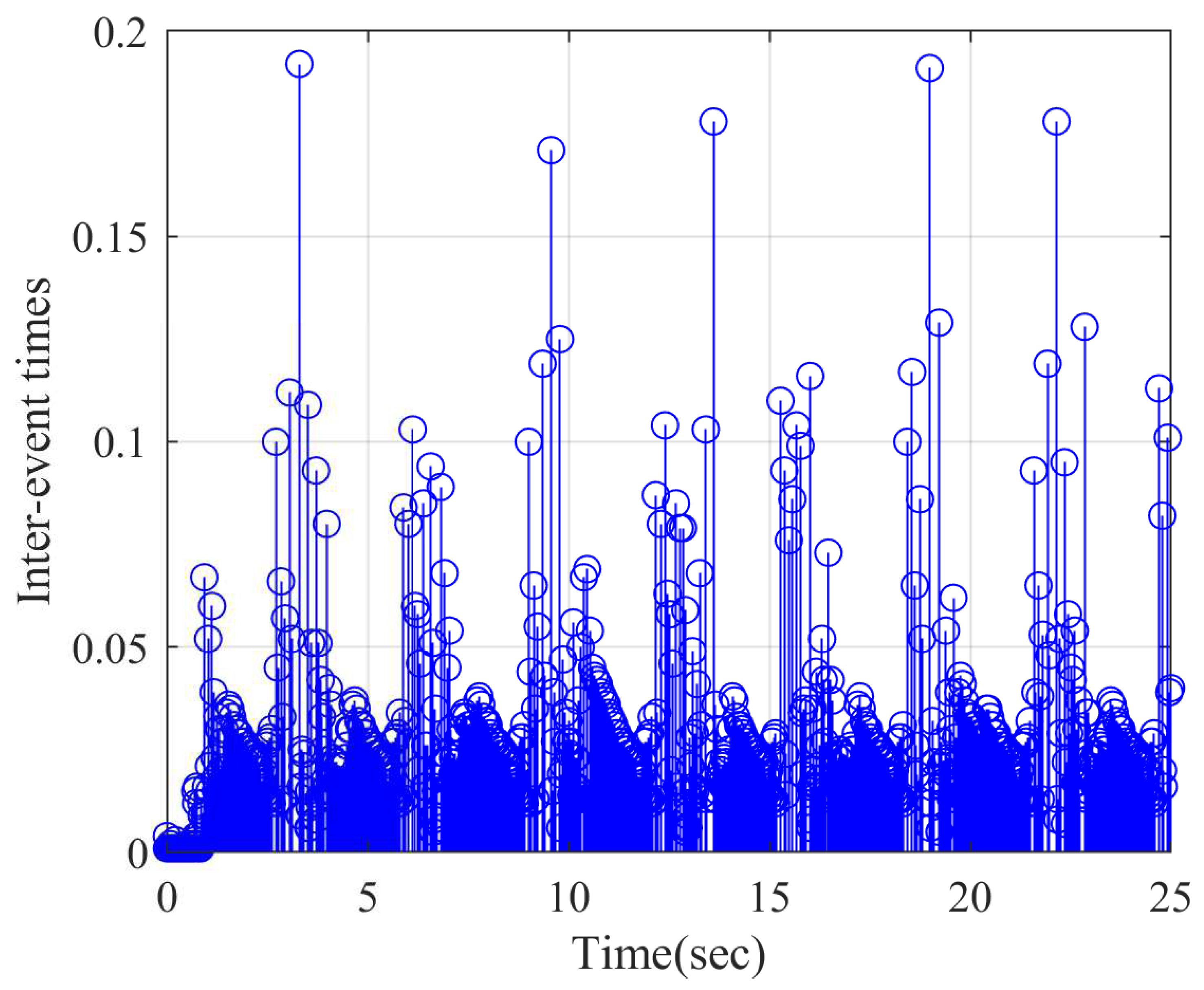
The Zeno behavior can be avoided.

5. Simulation

5.1. Example 1

A two-order pure-feedback FONS with full state constraints is described as

$$\left\{\begin{array}{c}{D}^{0.6}{x}_1=-0.5x_1^2+x_2+0.01sin\left(t\right)\hfill \\ D^{0.6}{x}_2=\frac{x_2-0.3x_1^2}{1+0.5x_1^4}-x_2+u\left(\nu \left(t-\tau \right)\right)+0.05cos\left(t\right)\hfill \end{array}\right.$$

where $f_1\left(x_1,x_2\right)=-0.5x_1^2+x_2$, $f_2\left(x_1,x_2\right)=\frac{x_2-0.3x_1^2}{1+0.5x_1^4}-x_2$, $\tau =0.01$, $d_1\left(t\right)=0.01sin\left(t\right)$ and $d_2\left(t\right)=0.05cos\left(t\right)$. $x_1$ and $x_2$ are the system states, which are confined as $\left|x_1\right|\le k_{c_1}=0.8$ and $\left|x_2\right|\le k_{c_2}=0.6$, respectively, and $y_r\left(t\right)=0.5sin\left(t\right)$. $\nu$ and $u\left(\nu \right)$ are the saturation input and output, and the saturation parameters are $u_{max}=0.8$ and $u_{min}=$$-0.5$.

Using the adaptive controller (14) and (48)–(51) with parameter-updated laws (15), (16), (46) and (47), the design parameters are chosen as $b_1=25,b_2=8,c_1=11,c_2=113,{\varphi }_1={\varphi }_2=1.01,{\gamma }_1=1.001,{\gamma }_2=1.101,{\xi }_1=11,{\xi }_2=111.1,{\delta }_1=1.1,{\phi }_1={\phi }_2={\varsigma }_1={\varsigma }_2=1.1,{\kappa }_2=0.06,{\kappa }^{*}=0.01,{\lambda }_1^{*}=0.001,{\lambda }_2^{*}=0.1$ and ${\overline{\lambda }}_2^{*}=0.2001$. Meanwhile, the initial values are selected as $x_1\left(0\right)=x_2\left(0\right)=0$, ${\theta }_1\left(0\right)={\theta }_2\left(0\right)=0$ and ${\varpi }_1\left(0\right)={\varpi }_2\left(0\right)=0$.

The simulation results are shown by Figure 2, Figure 3, Figure 4, Figure 5, Figure 6, Figure 7 and Figure 8. Figure 2 displays output tracking trajectories between the system output y and the reference signal $y_r$. Figure 3 shows the system states $x_2$. It is clear from these figures the full state constraints are not violated. The control input signals u shown in Figure 4, adaptive estimation for ${\theta }_1$ and ${\theta }_2$ shown in Figure 5, and ${\varpi }_1$ and ${\varpi }_2$ shown in Figure 6 are all bounded. Figure 7 lists the sequence of steps of event-triggered sampling to demonstrate the time interval results of the triggering events, and Figure 8 shows the number of accumulated events according to the event-triggered sampling in Figure 7, which can display that the proposed event-triggered controller can reduce the computational burden.

5.2. Example 2

In this example, the fractional-order Chua–Hartley system as a practical example is presented as follows [50]:

$$\left\{\begin{array}{c}{D}^{\alpha }{x}_1=\frac{10}{7}\left(x_1-x_1^3\right)+x_2+d_1\left(t\right)\hfill \\ D^{\alpha }{x}_2=10x_1-x_2+x_3+d_2\left(t\right)\hfill \\ D^{\alpha }{x}_3=-\frac{100}{7}{x}_2+u\left(\nu \left(t-\tau \right)\right)+d_3\left(t\right)\hfill \end{array}\right.$$

where $\alpha =0.98$, $f_1\left(x_1,x_2\right)=x_2+\frac{10}{7}\left(x_1-x_1^3\right)$, $f_2\left({\overline{x}}_2,x_3\right)=10x_1-x_2+x_3$, $f_3\left({\overline{x}}_3\right)=-\frac{100}{7}{x}_2$, and $\tau =0.005$. $d_1\left(t\right)=0.05cos\left(t\right),d_2\left(t\right)=0.1sin\left(t\right)$, and $d_3\left(t\right)=0.01\left(sin\left(t\right)+cos\left(t\right)\right)$ are the external disturbances. $x_1,x_2$, and $x_3$ are the system states, which are confined as $\left|x_1\right|\le k_{c_1}=0.9,\left|x_2\right|\le k_{c_2}=1.6$, and $\left|x_3\right|\le k_{c_3}=16$, respectively, and the desired signal is taken as $y_r\left(t\right)=0.8sin\left(t\right)$. The saturation parameters are $u_{max}=200$ and $u_{min}=$$-210$.

The design parameters are chosen as $b_1=16.1,b_2=31.1,b_3=71.1,c_1=1.1,c_2=c_3=101.8,{\varphi }_1={\varphi }_2={\varphi }_3=1.01,{\gamma }_1={\gamma }_2={\gamma }_3=0.001,{\xi }_1=11.1,{\xi }_2={\xi }_3=101.1,{\delta }_1={\delta }_2=1,{\phi }_1={\phi }_2={\phi }_3=1.1,{\varsigma }_1={\varsigma }_2={\varsigma }_3=0.01,{\kappa }_2={\kappa }_3=0.01,{\kappa }^{*}=0.01,{\lambda }_1^{*}=0.001,{\lambda }_2^{*}=1.1$, and ${\overline{\lambda }}_2^{*}=1.2011$. Meanwhile, the initial values are selected as $x_1\left(0\right)=x_2\left(0\right)=x_3\left(0\right)=0$, ${\theta }_1\left(0\right)={\theta }_2\left(0\right)={\theta }_3\left(0\right)=0$, and ${\varpi }_1\left(0\right)={\varpi }_2\left(0\right)={\varpi }_3\left(0\right)=0$.

To show the advantages of the proposed controller, a robust adaptive backstepping controller (RABC) in [52] is employed. Figure 9 shows the position relationship of y and $y_r$, in which the constraints are not violated. State $x_2$ is shown in Figure 10 and Figure 11, and $x_3$ is displayed in Figure 12 and Figure 13 by RABC and the proposed scheme, respectively. It is clear that the system states $x_2$ and $x_3$ by the proposed scheme satisfy the constraints $x_2<1.6$ and $x_3<16$. However, the system state $x_2$ and $x_3$ by the RABC violate the preset state constraints. The control input signals u shown in Figure 14, adaptive estimation for ${\theta }_1,{\theta }_2$, and ${\theta }_3$ shown in Figure 15, and ${\varpi }_1,{\varpi }_2$, and ${\varpi }_3$ shown in Figure 16 are all bounded. Figure 17 and Figure 18 show the sequence of steps of event-triggered sampling and the number of accumulated events to demonstrate the effectiveness of the computational burden reduction.

Based on the above simulation results, it can be observed by the proposed scheme that the tracking objective and the stability can be obtained, and reducing communication burden and meeting preset state limits can also be achieved.

6. Conclusions

An adaptive event-triggered controller approach for state-constrained pure-feedback FONSs with input delay, unknown actuator saturation, and external disturbances has been proposed. By employing the BLFs, backstepping technique, and auxiliary compensation system to handle input delay, the constraints are not violated. The fractional-order dynamic surface filters are used to deal with the complexity of the recursive procedure. The ETC strategy is applied to overcome the communication burden from the limited communication resources. The effectiveness can be verified by the simulation results. In the future, the controller design issue for time-delay switching FONSs will be considered, and the fractional-order circuit system will be built to verify the effectiveness of the proposed algorithm.

References

1. West, B.J.; Bologna, M.; Grigolini, P. Physics of Fractal Operators; Springer: Berlin/Heidelberg, Germany, 2003; Volume 10. [Google Scholar]
2. Bagley, R.L.; Torvik, P.J. On the fractional calculus model of viscoelastic behavior. J. Rheol. 1986, 30, 133–155. [Google Scholar] [CrossRef]
3. Li, Y.; Chen, Y.; Podlubny, I. Mittag-Leffler stability of fractional order nonlinear dynamic systems. Automatica 2009, 45, 1965–1969. [Google Scholar] [CrossRef]
4. Sun, H.; Zhang, Y.; Baleanu, D.; Chen, W.; Chen, Y. A new collection of real world applications of fractional calculus in science and engineering. Commun. Nonlinear Sci. Numer. Simul. 2018, 64, 213–231. [Google Scholar] [CrossRef]
5. Soleimanizadeh, A.; Nekoui, M.A. Optimal type-2 fuzzy synchronization of two different fractional-order chaotic systems with variable orders with an application to secure communication. Soft Comput. 2021, 25, 6415–6426. [Google Scholar] [CrossRef]
6. Li, X.; Mou, J.; Xiong, L.; Wang, Z.; Xu, J. Fractional-order double-ring erbium-doped fiber laser chaotic system and its application on image encryption. Opt. Laser Technol. 2021, 140, 107074. [Google Scholar] [CrossRef]
7. Shi, J.; He, K.; Fang, H. Chaos, Hopf bifurcation and control of a fractional-order delay financial system. Math. Comput. Simul. 2022, 194, 348–364. [Google Scholar] [CrossRef]
8. Wang, Y.L.; Jahanshahi, H.; Bekiros, S.; Bezzina, F.; Chu, Y.M.; Aly, A.A. Deep recurrent neural networks with finite-time terminal sliding mode control for a chaotic fractional-order financial system with market confidence. Chaos Solitons Fractals 2021, 146, 110881. [Google Scholar] [CrossRef]
9. Jin, T.; Xia, H.; Deng, W.; Li, Y.; Chen, H. Uncertain fractional-order multi-objective optimization based on reliability analysis and application to fractional-order circuit with caputo type. Circuits Syst. Signal Process. 2021, 40, 5955–5982. [Google Scholar] [CrossRef]
10. Mirzajani, S.; Aghababa, M.P.; Heydari, A. Adaptive T–S fuzzy control design for fractional-order systems with parametric uncertainty and input constraint. Fuzzy Sets Syst. 2018, 365, 22–39. [Google Scholar] [CrossRef]
11. Liu, H.; Li, S.; Wang, H.; Sun, Y. Adaptive fuzzy control for a class of unknown fractional-order neural networks subject to input nonlinearities and dead-zones. Inf. Sci. 2018, 454–455, 30–45. [Google Scholar] [CrossRef]
12. Song, S.; Park, J.H.; Zhang, B.; Song, X.; Zhang, Z. Adaptive Command Filtered Neuro-Fuzzy Control Design for Fractional-Order Nonlinear Systems With Unknown Control Directions and Input Quantization. IEEE Trans. Syst. Man Cybern. Syst. 2020, 51, 7238–7249. [Google Scholar] [CrossRef]
13. Hu, T.; He, Z.; Zhang, X.; Zhong, S. Event-triggered consensus strategy for uncertain topological fractional-order multiagent systems based on Takagi–Sugeno fuzzy models. Inf. Sci. 2021, 551, 304–323. [Google Scholar] [CrossRef]
14. Fei, J.; Wang, H.; Fang, Y. Novel neural network fractional-order sliding-mode control with application to active power filter. IEEE Trans. Syst. Man Cybern. Syst. 2021, 52, 3508–3518. [Google Scholar] [CrossRef]
15. Cao, B.; Nie, X. Event-triggered adaptive neural networks control for fractional-order nonstrict-feedback nonlinear systems with unmodeled dynamics and input saturation. Neural Netw. 2021, 142, 288–302. [Google Scholar] [CrossRef]
16. Liu, H.; Pan, Y.; Cao, J.; Wang, H.; Zhou, Y. Adaptive neural network backstepping control of fractional-order nonlinear systems with actuator faults. IEEE Trans. Neural Netw. Learn. Syst. 2020, 31, 5166–5177. [Google Scholar] [CrossRef] [PubMed]
17. Zhan, Y.; Tong, S. Adaptive fuzzy output-feedback decentralized control for fractional-order nonlinear large-scale systems. IEEE Trans. Cybern. 2021, 52, 12795–12804. [Google Scholar] [CrossRef]
18. Liu, Y.; Zhang, H.; Shi, Z.; Gao, Z. Neural-Network-Based Finite-Time Bipartite Containment Control for Fractional-Order Multi-Agent Systems. IEEE Trans. Neural Netw. Learn. Syst. 2022, 34, 7418–7429. [Google Scholar] [CrossRef]
19. Dhanalakshmi, P.; Senpagam, S.; Mohanapriya, R. Finite-time fuzzy reliable controller design for fractional-order tumor system under chemotherapy. Fuzzy Sets Syst. 2022, 432, 168–181. [Google Scholar] [CrossRef]
20. Wang, C.; Cui, L.; Liang, M.; Li, J.; Wang, Y. Adaptive Neural Network Control for a Class of Fractional-Order Nonstrict-Feedback Nonlinear Systems With Full-State Constraints and Input Saturation. IEEE Trans. Neural Netw. Learn. Syst. 2021, 33, 6677–6689. [Google Scholar] [CrossRef]
21. Zouari, F.; Ibeas, A.; Boulkroune, A.; Cao, J.; Arefi, M.M. Adaptive neural output-feedback control for nonstrict-feedback time-delay fractional-order systems with output constraints and actuator nonlinearities. Neural Netw. 2018, 105, 256–276. [Google Scholar] [CrossRef]
22. Shahvali, M.; Azarbahram, A.; Naghibi-Sistani, M.B.; Askari, J. Bipartite consensus control for fractional-order nonlinear multi-agent systems: An output constraint approach. Neurocomputing 2020, 397, 212–223. [Google Scholar] [CrossRef]
23. Zouari, F.; Ibeas, A.; Boulkroune, A.; Jinde, C.; Arefi, M.M. Neural network controller design for fractional-order systems with input nonlinearities and asymmetric time-varying Pseudo-state constraints. Chaos Solitons Fractals 2021, 144, 110742. [Google Scholar] [CrossRef]
24. Yu, Z.; Zhang, Y.; Jiang, B.; Su, C.Y.; Fu, J.; Jin, Y.; Chai, T. Nussbaum-based finite-time fractional-order backstepping fault-tolerant flight control of fixed-wing UAV against input saturation with hardware-in-the-loop validation. Mech. Syst. Signal Process. 2021, 153, 107406. [Google Scholar] [CrossRef]
25. Alipour, M.; Malekzadeh, M.; Ariaei, A. Active fractional-order sliding mode control of flexible spacecraft under actuators saturation. J. Sound Vib. 2022, 535, 117110. [Google Scholar] [CrossRef]
26. Ju, X.; Wei, C.; Xu, H.; Wang, F. Fractional-order sliding mode control with a predefined-time observer for VTVL reusable launch vehicles under actuator faults and saturation constraints. ISA Trans. 2022, 129, 55–72. [Google Scholar] [CrossRef] [PubMed]
27. Geng, W.T.; Lin, C.; Chen, B. Observer-based stabilizing control for fractional-order systems with input delay. ISA Trans. 2020, 100, 103–108. [Google Scholar] [CrossRef]
28. Keighobadi, J.; Pahnehkolaei, S.M.A.; Alfi, A.; Machado, J. Command-filtered compound FAT learning control of fractional-order nonlinear systems with input delay and external disturbances. Nonlinear Dyn. 2022, 108, 293–313. [Google Scholar] [CrossRef]
29. Zirkohi, M.M. Robust adaptive backstepping control of uncertain fractional-order nonlinear systems with input time delay. Math. Comput. Simul. 2022, 196, 251–272. [Google Scholar] [CrossRef]
30. Liu, S.; Wang, H.; Li, T. Adaptive composite dynamic surface neural control for nonlinear fractional-order systems subject to delayed input. ISA Trans. 2022, 134, 122–133. [Google Scholar] [CrossRef]
31. Zou, W.; Mao, J.; Xiang, Z. Adaptive Fuzzy Finite-Time Sampled-Data Control for A Class of Fractional-Order Nonlinear Systems. IEEE Trans. Fuzzy Syst. 2024, 1–14. [Google Scholar] [CrossRef]
32. Ha, S.; Chen, L.; Liu, D.; Liu, H. Command Filtered Adaptive Fuzzy Control of Fractional-Order Nonlinear Systems with Unknown Dead Zones. IEEE Trans. Syst. Man Cybern. Syst. 2024, 1–12. [Google Scholar] [CrossRef]
33. Li, D.; Dong, J. Fractional-Order Systems Optimal Control via Actor-Critic Reinforcement Learning and Its Validation for Chaotic MFET. IEEE Trans. Autom. Sci. Eng. 2024, 1–10. [Google Scholar] [CrossRef]
34. Xing, Y.; Wang, Y. Finite-Time Adaptive NN Backstepping Dynamic Surface Control for Input-Delay Fractional-Order Nonlinear Systems. IEEE Access 2023, 11, 5206–5214. [Google Scholar] [CrossRef]
35. Podlubny, I. Fractional Differential Equations; Academic Press: Cambridge, MA, USA, 1999; p. 2. [Google Scholar]
36. Das, S. Functional Fractional Calculus for System Identification and Controls; Springer: Berlin/Heidelberg, Germany, 2008. [Google Scholar]
37. Duarte-Mermoud, M.A.; Aguila-Camacho, N.; Gallegos, J.A.; Castro-Linares, R. Using general quadratic Lyapunov functions to prove Lyapunov uniform stability for fractional order systems. Commun. Nonlinear Sci. Numer. Simul. 2015, 22, 650–659. [Google Scholar] [CrossRef]
38. Aguila Camacho, N.; Duarte Mermoud, M.A.; Gallegos, J.A. Lyapunov functions for fractional order systems. Commun. Nonlinear Sci. Numer. Simul. 2014, 19, 2951–2957. [Google Scholar] [CrossRef]
39. Chen, W.; Dai, H.; Song, Y.; Zhang, Z. Convex Lyapunov functions for stability analysis of fractional order systems. IET Control Theory Appl. 2017, 11, 1070–1074. [Google Scholar] [CrossRef]
40. Gong, P. Distributed tracking of heterogeneous nonlinear fractional-order multi-agent systems with an unknown leader. J. Frankl.-Inst.-Eng. Appl. Math. 2017, 354, 2226–2244. [Google Scholar] [CrossRef]
41. Ren, B.; Ge, S.S.; Tee, K.P.; Lee, T.H. Adaptive Neural Control for Output Feedback Nonlinear Systems Using a Barrier Lyapunov Function. IEEE Trans. Neural Netw. 2010, 21, 1339–1345. [Google Scholar]
42. Tee, K.P.; Ge, S.S.; Tay, E.H. Barrier Lyapunov Functions for the control of output-constrained nonlinear systems. Automatica 2009, 45, 918–927. [Google Scholar] [CrossRef]
43. Polycarpou, M.M. Stable adaptive neural control scheme for nonlinear systems. IEEE Trans. Autom. Control 1996, 41, 447–451. [Google Scholar] [CrossRef]
44. Sanner, R.M.; Slotine, J.J. Gaussian networks for direct adaptive control. IEEE Trans. Neural Netw. 1992, 3, 837–863. [Google Scholar] [CrossRef] [PubMed]
45. Wang, H.; Chen, B.; Liu, X.; Liu, K.; Lin, C. Robust Adaptive Fuzzy Tracking Control for Pure-Feedback Stochastic Nonlinear Systems With Input Constraints. IEEE Trans. Cybern. 2013, 43, 2093–2104. [Google Scholar] [CrossRef] [PubMed]
46. Yu, J.; Shi, P.; Dong, W.; Lin, C. Command Filtering-Based Fuzzy Control for Nonlinear Systems with Saturation Input. IEEE Trans. Cybern. 2017, 47, 2472–2479. [Google Scholar] [CrossRef] [PubMed]
47. Shao, S.; Chen, M.; Chen, S.; Wu, Q. Adaptive neural control for an uncertain fractional-order rotational mechanical system using disturbance observer. IET Control Theory Appl. 2016, 10, 1972–1980. [Google Scholar] [CrossRef]
48. Xu, B.; Chen, D.; Zhang, H.; Wang, F. Modeling and stability analysis of a fractional-order Francis hydro-turbine governing system. Chaos Solitons Fractals 2015, 75, 50–61. [Google Scholar] [CrossRef]
49. Ni, J.; Liu, L.; Liu, C.; Hu, X. Fractional order fixed-time nonsingular terminal sliding mode synchronization and control of fractional order chaotic systems. Nonlinear Dyn. 2017, 89, 2065–2083. [Google Scholar] [CrossRef]
50. Petras, I. A note on the fractional-order Chua’s system. Chaos Solitons Fractals 2008, 38, 140–147. [Google Scholar] [CrossRef]
51. Wang, M.; Liu, X.; Shi, P. Adaptive Neural Control of Pure-Feedback Nonlinear Time-Delay Systems via Dynamic Surface Technique. IEEE Trans. Syst. Man Cybern. Part B 2011, 41, 1681–1692. [Google Scholar] [CrossRef]
52. Jafari, A.A.; Mohammadi, S.M.A.; Naseriyeh, M.H. Adaptive type-2 fuzzy backstepping control of uncertain fractional-order nonlinear systems with unknown dead-zone. Appl. Math. Model. 2019, 69, 506–532. [Google Scholar] [CrossRef]
Figure 1. The block diagram of the proposed controller.
Fractalfract 08 00256 g001
Figure 2. Output y and tracking signal y r t .
Fractalfract 08 00256 g002
Figure 3. State x 2 .
Fractalfract 08 00256 g003
Figure 4. Control input u.
Fractalfract 08 00256 g004
Figure 5. Parameter estimation θ 1 and θ 2 .
Fractalfract 08 00256 g005
Figure 6. Parameter estimation ϖ 1 and ϖ 2 .
Fractalfract 08 00256 g006
Figure 7. Time interval.
Fractalfract 08 00256 g007
Figure 8. Cumulative number of events.
Fractalfract 08 00256 g008
Figure 9. Output y and tracking signal y r t .
Fractalfract 08 00256 g009
Figure 10. State x 2 .
Fractalfract 08 00256 g010
Figure 11. State x 2 .
Fractalfract 08 00256 g011
Figure 12. State x 3 .
Fractalfract 08 00256 g012
Figure 13. State x 3 .
Fractalfract 08 00256 g013
Figure 14. Control input u.
Fractalfract 08 00256 g014
Figure 15. Parameter estimation θ 1 , θ 2 , and θ 3 .
Fractalfract 08 00256 g015
Figure 16. Parameter estimation ϖ 1 , ϖ 2 , and ϖ 3 .
Fractalfract 08 00256 g016
Figure 17. Time interval.
Fractalfract 08 00256 g017
Figure 18. Cumulative number of events.
Fractalfract 08 00256 g018
Disclaimer/Publisher’s Note: The statements, opinions and data contained in all publications are solely those of the individual author(s) and contributor(s) and not of MDPI and/or the editor(s). MDPI and/or the editor(s) disclaim responsibility for any injury to people or property resulting from any ideas, methods, instructions or products referred to in the content.