Numerical Simulation and Parameter Estimation of the Space-Fractional Magnetohydrodynamic Flow and Heat Transfer Coupled Model

Abstract

In this paper, a coupled model is built to research the space-fractional magnetohydrodynamic (MHD) flow and heat transfer problem. The fractional coupled model is solved numerically by combining the matrix function vector products method in the temporal direction with the spectral method in the spatial direction. A fast method based on the numerical scheme is established to reduce the computational time. With the help of the Bayesian method, the space-fractional orders of the coupled model are estimated, and the problem of multi-parameter estimation in the coupled model is solved. Finally, a numerical example is carried out to verify the stability of the numerical methods and the effectiveness of the parameter estimation method. Results show that the numerical method is stable, which converges with an accuracy of $O({\tau }^2+N^{-r})$. The fast method is efficient in reducing the computational time, and the parameter estimation method can effectively estimate parameters in the space-fractional coupled model. The numerical solutions are discussed to describe the effects of several important parameters on the velocity and the temperature. Results indicate that the Lorentz force produced by the MHD flow blocks the movement of the fluid and prolongs the time for the fluid to reach a stable state. But the Hall parameter m weakens this hindrance. The Joule heating effects play a negative role in heat transfer.

1. Introduction

In recent years, the magnetohydrodynamic (MHD) flow and heat transfer processes have garnered wide concern because of its various applications, such as nuclear reactor, physics, and ocean dynamics [1,2,3,4]. The MHD coupled model is a physical model that can describe the interaction between magnetic field and fluid motion. In the MHD model, the fluid is assumed to be an electrical conductor, which can induce a magnetic field, while the magnetic field can also exert force on the fluid. The fractional models play important roles in the study of MHD flow and heat transfer. Chen et al. [5] researched the boundary layer flow of viscoelastic MHD fluid over a stretching sheet with a double fractional Maxwell model, and indicated the influence of fractional parameters on the flow. In this work, we build a space-fractional coupled model to discuss the MHD flow and heat transfer process. The fractional MHD coupled model provides a theoretical framework for describing and explaining the interactions between complex magnetic fields and fluids, providing us with powerful tools for explaining many phenomena in nature and developing new technological applications. Previously, most studies on MHD flow had overlooked the effect of induced magnetic fields, but in practical applications, this effect should not be ignored. Therefore, we consider the influence of induced magnetic fields on the MHD flow processes.

Many researchers have paid attention to the numerical method of solving the fractional model [6,7,8]. Zeng et al. [9] proposed a corrected L1 method to discretize the Caputo fractional derivative operator approximately. Wang et al. [10] developed a FDM to study the non-Fourier bioheat transfer process. However, traditional numerical methods to solve the fractional equation need a lot of computational time and have many memory requirements, especially in solving fractional coupled equations. In recent years, many scholars have focused on the fast method for solving the fractional coupled model. Using the principle of efficient sum-of-exponentials (SOE) approximation, Jia et al. [11] solved the the 2D nonlinear time–space-fractional coupled Klein–Gordon–Zakharov (KGZ) equations, and illustrated the efficiency of the fast method. Jian et al. [12] constructed a fast and efficient numerical method to solve nonlinear space-fractional multi-delay reaction–diffusion equations.

In the meantime, the identification of the model parameters has been paid more and more attention by experts and scholars. How to estimate parameters in the fractional model has become significantly important [13,14,15]. For an uncertain differential equation, Yang et al. [16] firstly investigated the parameter estimation problem. Yang et al. [17] obtained the physical parameters of the fractional fractal diffusion model by comparing and contrasting several parameter estimating methods. Recently, with the adsorption experimental heat flux data, Chi et al. [18] proposed the cuckoo search algorithm to estimate the parameters of fractional heat conduction model. However, there is relatively little research on the problem of multi-parameter estimation in the coupled model. We propose a multi-parameter estimation method based on Bayesian technology, which can effectively solve this problem.

The two main contributions of this work can be summarized as follows. First, we introduce a numerical method for solving the space-fractional MHD coupled model and propose a fast method to reduce computational time and enhance efficiency. This is necessary because the computational cost of the existing numerical methods for fractional equations, especially for space-fractional coupled models, is very high. Second, we propose a multi-parameter estimation method based on the Bayesian technology and use this method to estimate the fractional derivative parameters of the space-fractional MHD coupled model, which can make the analysis more accurate. The correct parameters can help us analyze the MHD flow and heat transfer process more accurately. This multi-parameter estimation method can be used to solve the multi-parameter estimation problem of other space-fractional coupled models, providing a framework for studying the MHD flow and heat transfer problems of space-fractional fluid.

This study proposes the space-fractional coupled model and then builds a numerical method to solve the model. A fast method is presented to reduce the computational time. We also provide a parameter estimation method based on the Bayesian method. The rest of this paper is organized as follows: Section 2 proposes the mathematical model, and Section 3 builds the numerical scheme. Section 4 presents the numerical scheme and the fast method for solving the model. The parameter estimation technique is outlined in Section 5. Section 6 then offers a specific example to demonstrate the efficiency of the numerical scheme, the fast method, and the parameter estimation technique. Additionally, this section provides an analysis of the influence of critical parameters on fluid dynamics and heat transfer. Finally, the findings are summarized in the subsequent Section 7.

2. Mathematical Model

In this section, we will explain the space-fractional coupled model addressed in this paper. The momentum equation for MHD fluids describes the motion of a conducting fluid influenced by both magnetic and hydrodynamic forces. Assuming that the incompressible magnetic fluid follows the Boussinesq approximation, the momentum equation can be expressed as follows [19]:

$$\begin{array}{cc}\hfill & \nabla ·\mathbf{u}=0,\hfill \\ \hfill & \rho \left({\displaystyle \frac{\partial \mathbf{u}}{\partial t}}+(\mathbf{u}·\nabla )\mathbf{u}-(\mathbf{b}·\nabla )\mathbf{b}\right)=\nabla ·\mathbf{S}+\rho \mathbf{g}{\beta }_{T}T+\mathbf{J}\times \mathbf{b},\hfill \end{array}$$

(1)

where $\mathbf{u}$ (m/s) is the velocity vector, $\mathbf{b}$ is the magnetic field vector, $\mathbf{S}$ is the Cauchy stress tensor, T is the temperature, $\rho$ is the density of the fluid, ${\beta }_T$ stands for the coefficient of thermal expansion, $\mathbf{g}$ stands for the gravitational acceleration vector, $\mathbf{J}$ is the current density vector, and ∇ is the gradient operator. In the following discussion, we posit that the gravitational acceleration vector is aligned with the velocity vector, while the magnetic field vector is perpendicular to the direction of the velocity vector. For the viscoelastic dynamics of magneto-fluids, many experts and scholars have introduced fractional operators instead of integral operators in the classical fluid model to describe the constitutive equation. The space-fractional constitutive model without the pressure of the fluid is [20]

$$\mathbf{S}={\nu }_{\alpha }{\nabla }^{\alpha -1}\mathbf{u},$$

(2)

in which ${\nu }_{\alpha }$ is the fractional dynamic viscosity, $\alpha$ is the fractional-order parameter, and ${\nabla }^{\alpha -1}$ is the fractional gradient operator. The interaction between a magnetic field and a fluid results in the generation of a force known as the Lorentz force. This force is contingent upon the fluid’s conductivity, velocity, and the magnetic field’s strength. This can lead to phenomena such as fluid acceleration, deceleration, and the generation of vortices and turbulence. Considering the Hall effects and ignoring the the influence of electric field, the generalized Ohm’s law can be written as

$$\mathbf{J}+{\xi }_h(\mathbf{J}\times \mathbf{b})={\sigma }_h(\mathbf{u}\times \mathbf{b}),$$

(3)

in which ${\xi }_h$ is the parameter of the Hall effects, and ${\sigma }_h$ is the conductivity of the fluid. It is clear that when the magnetism of a magnetic fluid is high, the induced magnetic field generated during the flow process also affects the MHD flow and heat transfer. This induction is described by Faraday’s law of induction. This indicates a close coupling between the velocity of the fluid and the magnetic field. We consider the following magnetic equation with space-fractional magnetic diffusion [21]:

$${\displaystyle \frac{\partial \mathbf{b}}{\partial t}}+(\mathbf{u}·\nabla )\mathbf{b}-(\mathbf{b}·\nabla )\mathbf{u}+{\mu }_{\beta }{(-\Delta )}^{\beta /2}\mathbf{b}=0,$$

(4)

where $\beta$ is the fractional-order parameter, ${\mu }_{\beta }$ is the magnetic field viscosity coefficient, and ${(-\Delta )}^{\beta /2}$ is the fractional Laplace operator. In the process of MHD flow, the heat transfer phenomenon is often accompanied, and correspondingly, changes in fluid temperature can also affect the flow of the fluid. Among them, the Joule heating effects play an important role. Therefore, we need to consider the energy equation with the Joule heating effects to study the MHD flow and heat transfer of the fluid. The space-fractional energy equation with the Joule heating effects is given as [22]

$$\rho C_p\left({\displaystyle \frac{\partial T}{\partial t}}+(\mathbf{u}·\nabla )T\right)+{\upsilon }_{\gamma }{(-\Delta )}^{\gamma /2}T=R_j,$$

(5)

where $\gamma$ is the fractional-order parameter, $C_p$ is the heat capacity, and ${\upsilon }_{\gamma }$ is the thermal conductivity. $R_j$ is the Joule heating effects denoted by $R_j={\displaystyle \frac{1}{{\sigma }_h}}{\mathbf{J}}^2$.

For simplicity, we introduce the following dimensionless quantities:

$$x^{\ast }={\displaystyle \frac{x}{h}},y^{\ast }={\displaystyle \frac{y}{h}},z^{\ast }={\displaystyle \frac{z}{h}},t^{\ast }={\displaystyle \frac{U_{0}t}{h}},u^{\ast }={\displaystyle \frac{u}{U_0}},b^{\ast }={\displaystyle \frac{b}{B_0}},\theta ={\displaystyle \frac{T}{T_0}},\nu ={\displaystyle \frac{{\nu }_{\alpha }}{\rho h^{\alpha -1}{U}_0}},$$

$$\mu ={\displaystyle \frac{{\mu }_{\beta }}{h^{\beta -1}{U}_0}},K_{\gamma }={\displaystyle \frac{{\upsilon }_{\gamma }}{\rho C_p{h}^{\gamma -1}{U}_0}},Gr={\displaystyle \frac{g{\beta }_{T}h{T}_0}{U_0^2}},M={\displaystyle \frac{{\sigma }_h{B}_0^{2}h}{\rho U_0}},m={\xi }_h^2{B}_0^2,H_{\gamma }={\displaystyle \frac{{\sigma }_h{U}_0{B}_0^{2}h}{\rho C_p{T}_0}},$$

where h is the characteristic length, $U_0$ is the characteristic velocity, $B_0$ is the characteristic magnetic field, and $T_0$ is the characteristic temperature. $\nu$ and $\mu$ are the viscosity parameter of velocity and the magnetic field, respectively. $K_{\gamma }$ is the parameter representing the relationship between the energy and momentum transfer, $G_r$ is the Grashof number, M is the Hartmann number, m is the Hall parameter, and $H_{\gamma }$ is the Joule thermal parameter. For simplicity, we take $B_0^2/U_0^2=1$. Because in a strong magnetic field state, there is a close correlation between velocity and magnetic field at the initial moment, the tension of the magnetic field can be counteracted by the motion of the fluid. That is to say, the velocity field and magnetic field reach an equilibrium state. Considering the velocity and magnetic field in a certain direction and through variable transformation, we can obtain the following 2D dimensionless coupled equations:

$$\begin{array}{c}\hfill {\displaystyle \frac{\partial u}{\partial t}}+u{\nabla }_{d}u-b{\nabla }_{d}b+\nu {(-\Delta )}^{\alpha /2}u=G_r\theta -{\displaystyle \frac{M{b}^2}{1+m^2{b}^2}}u,\end{array}$$

(6)

$${\displaystyle \frac{\partial b}{\partial t}}+u{\nabla }_{d}b-b{\nabla }_{d}u+\mu {(-\Delta )}^{\beta /2}b=0,$$

(7)

$${\displaystyle \frac{\partial \theta }{\partial t}}+u{\nabla }_d\theta +K_{\gamma }{(-\Delta )}^{\gamma /2}\theta ={\displaystyle \frac{H_{\gamma }{b}^2}{1+m^2{b}^2}}{u}^2,$$

(8)

$$\begin{array}{c}\hfill u(x,y,t)=b(x,y,t)=\theta (x,y,t)=0,(x,y)\in \partial \Omega ,0\le t\le \tilde{T},\end{array}$$

(9)

$$\begin{array}{c}\hfill u(x,y,0)=u_0(x,y),b(x,y,0)=b_0(x,y),\theta (x,y,0)={\theta }_0(x,y),(x,y)\in \overline{\Omega },\end{array}$$

(10)

such that $(x,y)\in \Omega ,0<t\le \tilde{T}$, and $\tilde{T}$ is the final time. Here, ${\nabla }_d$ is the first-order differential operator in direction $d=\{x,y,z\}$; u and b are the velocity and magnetic field in a certain direction; $\theta$ is the temperature of fluid; and $u_0$, $b_0$, and ${\theta }_0$ are the initial condition functions of the velocity, magnetic field, and temperature. The space-fractional operators ${(-\Delta )}^{\alpha /2}$, ${(-\Delta )}^{\beta /2}$ and ${(-\Delta )}^{\gamma /2}$ are the 2D fractional Laplace operators of order $1<\alpha ,\beta ,\gamma \le 2$. And for any function $f(x,y)$ and $1<\sigma \le 2$, ${(-\Delta )}^{\sigma /2}f(x,y)$ can be defined as [23]

$${(-\Delta )}^{\sigma /2}f(x,y)=\sum _{i=1}^{\infty }\sum _{j=1}^{\infty }{\widehat{f}}_{ij}{\left({\lambda }_{ij}\right)}^{\sigma /2}{\varphi }_{ij}(x,y),$$

(11)

where ${\widehat{f}}_{ij}=(f,{\varphi }_{ij})$. $({\lambda }_{ij},{\varphi }_{ij})$$(i,j=1,2,\cdots )$ are the eigenvalues and orthogonal eigenfunctions of the standard Laplacian $(-\Delta )$ under the corresponding homogeneous boundary condition on $\Omega$, i.e., $(-\Delta ){\varphi }_{ij}={\lambda }_{ij}{\varphi }_{ij}$.

3. Preliminary

In this section, we provide the matrix function vector products method (MFVPM) to solve the space-fractional equation [24]. Let A be the approximate matrix, $\mathbf{r}$ be the vector, and $\Lambda$ and Q be the diagonal matrix and orthogonal eigenvectors matrix of A, respectively. Due to the Cauchy integral formula, an analytic function f of A multiplied by $\mathbf{r}$ can be written as

$$f\left(A\right)\mathbf{r}={\displaystyle \frac{1}{2\pi i}}{\oint }_{C}f\left(z\right){(zI-A)}^{-1}\mathbf{r}dz,$$

(12)

where C is a known closed contour, and i is the imaginary unit. Through conformal mapping $z\left(\zeta \right)=\sqrt{{\lambda }_1{\lambda }_N}\left({\displaystyle \frac{k^{-1}+\mathrm{sn}\left(\zeta \right)}{k^{-1}-\mathrm{sn}\left(\zeta \right)}}\right)$, we can rewrite Equation (12) as

$$f\left(A\right)\mathbf{r}=\mathrm{Im}{\int }_{-\mathrm{K}+{\mathrm{iK}}^{\prime }/2}^{\mathrm{K}+{\mathrm{iK}}^{\prime }/2}\omega \left(\tau \right){(\mathrm{z}\left(\zeta \right)\mathrm{I}-\mathrm{A})}^{-1}\mathbf{r}\mathrm{d}\zeta ,$$

(13)

where $\omega \left(\zeta \right)={\displaystyle \frac{-2\sqrt{{\lambda }_1{\lambda }_N}f\left(z\left(\zeta \right)\right)\mathrm{cn}\left(\zeta \right)\mathrm{dn}\left(\zeta \right)}{\pi k{(k^{-1}-\mathrm{sn}\left(\zeta \right))}^2}}$, $k={\displaystyle \frac{\sqrt{\kappa }-1}{\sqrt{\kappa }+1}}$, and $\kappa ={\displaystyle \frac{{\lambda }_N}{{\lambda }_1}}$. ${\lambda }_1$ and ${\lambda }_N$ are the smallest and largest eigenvalues of A, respectively. $\mathrm{sn}\left(\zeta \right)$, $\mathrm{cn}\left(\zeta \right)$, and $\mathrm{dn}\left(\zeta \right)$ are the Jacobi elliptic functions. K and $K^{\prime }$ are defined by full elliptic integrals with k and $k^{\prime }=\sqrt{1-k^2}$. We use the midpoint rule to approximate Equation (13) as  

$$f\left(A\right)\mathbf{r}\approx \mathrm{Im}\sum _{\mathrm{j}=1}^{\mathrm{P}}{\omega }_{\mathrm{j}}{({\mathrm{z}}_{\mathrm{j}}\mathrm{I}-\mathrm{A})}^{-1}\mathbf{r},$$

(14)

in which ${\omega }_j={\displaystyle \frac{-4K\sqrt{{\lambda }_1{\lambda }_N}f\left(z\left({\zeta }_j\right)\right)\mathrm{cn}\left({\zeta }_{\mathrm{j}}\right)\mathrm{dn}\left({\zeta }_{\mathrm{j}}\right)}{\pi Pk{(k^{-1}-\mathrm{sn}\left({\zeta }_{\mathrm{j}}\right))}^2}}$, $z_j=z\left({\zeta }_j\right)$. P is the number of quadrature points, and ${\zeta }_j$ are the summation points. Next, we use the symmetric Lanczos algorithm to solve ${(z_{j}I-A)}^{-1}\mathbf{r}$. With $A\in {\mathbb{R}}^{N\times N}$ and $\mathbf{r}\in {\mathbb{R}}^N$, we can obtain the solutions of linear systems $(z_{j}I-A)\mathbf{x}=\mathbf{r}$ as ${\mathbf{x}}_{\tilde{m}}={\parallel \mathbf{r}\parallel }_2{V}_{\tilde{m}}{(z_{j}I-T_{\tilde{m}})}^{-1}{\mathbf{e}}_1$, where $V_{\tilde{m}}$ and $T_{\tilde{m}}$ are computed by the symmetric Lanczos algorithm. $\tilde{m}$ is the dimension of the corresponding Krylov subspace $\mathcal{K}(A,\mathbf{r})$ [24], which can be calculated by the error bound of the Lanczos algorithm and tolerance $e_{tol}$.

In practical applications, the computational costs of the above method is expensive, and thus it cannot be well utilized and promoted. In order to reduce the computational costs and improve the computational efficiency, a fast method (MFVPM-l) based on the l accelerate algorithm and polynomial processing method is considered. We recompute a set of lth orthogonal eigenvectors corresponding to the smallest lth eigenvalue of A, and Equation (14) can be approximated as

$$f\left(A\right)\mathbf{r}\approx Q_{l}f\left({\Lambda }_l\right)Q_l^T\mathbf{r}+\mathrm{Im}\sum _{\mathrm{j}=1}^{\mathrm{P}}{\omega }_{\mathrm{j}}{\mathbf{x}}_{\mathrm{j}},$$

(15)

where ${\omega }_j$ are the weight of quadrature, ${\mathbf{x}}_j$ are the solutions of systems $(z_{j}I-\widehat{A}){\mathbf{x}}_j=\widehat{\mathbf{r}}$, and $\widehat{\mathbf{r}}=(I-Q_l{Q}_l^T)\mathbf{r}$. $\widehat{A}$ is the deflated matrix built by mapping the smallest l eigenvalues of A to a chosen value ${\lambda }^{\ast }$ defined as $\widehat{A}=A+Q_l({\lambda }^{\ast }I-{\Lambda }_l)Q_l^T$ [25,26], and l is a positive integer. We can recalculate the modified values of $\tilde{m}$ by using the error bound of the Lanczos algorithm and the given tolerance $e_{tol}$, and l satisfies that minimizes $l+2\tilde{m}$, where $\kappa ={\lambda }_N/{\lambda }_{l+1}$.

Suppose that there are two polynomial functions $p_{z_j}\left(x\right)$ and $p\left(x\right)$ of degree q satisfying $\mathcal{K}((z_{j}I-\widehat{A})p_{z_j}\left(\widehat{A}\right),\widehat{\mathbf{r}})=\mathcal{K}(\widehat{A}p\left(\widehat{A}\right),\widehat{\mathbf{r}})$. Let $p\left(x\right)$ be the least squares polynomial with the Jacobi weight $({\displaystyle \frac{1}{2}},{\displaystyle \frac{1}{2}})$ and $p_{z_j}\left(x\right)$ be the modified polynomial function on $z_j$. Assuming that there is a parameter ${\overline{\omega }}_{z_j}$ dependent on $z_j$ such that $(z_{j}I-\widehat{A})p_{z_j}\left(\widehat{A}\right)={\overline{\omega }}_{z_j}I-\widehat{A}p\left(\widehat{A}\right)$, we can obtain the representations of $p_{z_j}\left(x\right)$ and ${\overline{\omega }}_{z_j}$. We build the modified Lanczos decomposition

$$\widehat{A}p\left(\widehat{A}\right)V_{\tilde{m}}^0=V_{\tilde{m}}^0{T}_{\tilde{m}}^0+{\eta }_{\tilde{m}+1}^0{\mathbf{v}}_{\tilde{m}+1}^0{\mathbf{e}}_{\tilde{m}}^T.$$

(16)

Therefore, the approximate solutions can be written as

$${\mathbf{x}}_j\approx \parallel \widehat{\mathbf{r}}\parallel p_{z_j}\left(\widehat{A}\right)V_{\tilde{m}}^0{({\overline{\omega }}_{z_j}I-T_{\tilde{m}}^0)}^{-1}{\mathbf{e}}_1.$$

(17)

4. Materials and Methods

To better study the numerical method for solving the fractional coupled model mentioned above, the stability and convergence of the solving scheme are demonstrated, and the MHD flow and heat transfer under different conditions are discussed. We add a source term at the right end of Equations (6)–(8). The source term is mainly used to describe the external excitation or influence that the system is subjected to, and plays an important role in describing external forcing, as well as giving precise solutions to equilibrium equations. In this section, we examine the following 2D space-fractional coupled equations:

$$\begin{array}{c}\hfill {\displaystyle \frac{\partial u}{\partial t}}+u{\nabla }_{d}u-b{\nabla }_{d}b+\nu {(-\Delta )}^{\alpha /2}u=G_r\theta -{\displaystyle \frac{M{b}^2}{1+m^2{b}^2}}u+g_1(x,y,t),\end{array}$$

(18)

$${\displaystyle \frac{\partial b}{\partial t}}+u{\nabla }_{d}b-b{\nabla }_{d}u+\mu {(-\Delta )}^{\beta /2}b=g_2(x,y,t),$$

(19)

$$\begin{array}{c}\hfill {\displaystyle \frac{\partial \theta }{\partial t}}+u{\nabla }_d\theta +K_{\gamma }{(-\Delta )}^{\gamma /2}\theta ={\displaystyle \frac{H_{\gamma }{b}^2}{1+m^2{b}^2}}{u}^2+g_3(x,y,t),\end{array}$$

(20)

subject to the boundary conditions

$$\begin{array}{c}\hfill u(x,y,t)=b(x,y,t)=\theta (x,y,t)=0,(x,y)\in \partial \Omega ,0\le t\le \tilde{T},\end{array}$$

(21)

and the initial conditions

$$\begin{array}{c}\hfill u(x,y,0)=u_0(x,y),b(x,y,0)=b_0(x,y),\theta (x,y,0)={\theta }_0(x,y),(x,y)\in \overline{\Omega },\end{array}$$

(22)

where $(x,y)\in \Omega$, $0\le t\le \tilde{T}$. $\nu$, $\mu$, $K_{\gamma }$, $G_r$, M, m, and $H_{\gamma }$ are the positive parameters; $g_1(x,y,t)$, $g_2(x,y,t)$, $g_3(x,y,t)$, and $u_0(x,y)$, $b_0(x,y)$, ${\theta }_0(x,y)$ are the given functions. And the orders of the space-fractional operators satisfy $1<\alpha ,\beta ,\gamma \le 2$. In this section, the numerical method is built to solve Equations (18)–(22). In addition, we propose a fast method for solving the coupled model to reduce the computational cost.

Let $t\in (0,\tilde{T}]$, $t_n=n\tau$, $n=0,1,\cdots ,n_{\tilde{T}}$, where $\tau =\tilde{T}/n_{\tilde{T}}$ is the time-step and $n_{\tilde{T}}$ is a positive integer. Denote $u^n=u^n(·,·)=u(·,·,t_n)$, $b^n=b^n(·,·)=b(·,·,t_n)$ and ${\theta }^n={\theta }^n(·,·)=\theta (·,·,t_n)$. For convenience, we introduce the following notations for any smooth function v:

$$D_1{v}^1={\displaystyle \frac{v^1-v^0}{\tau }},D_2{v}^n={\displaystyle \frac{3v^n-4v^{n-1}+v^{n-2}}{2\tau }},n\ge 2.$$

(23)

Then, we can obtain the approximation ${\displaystyle \frac{\partial v}{\partial t}=\left\{\begin{array}{c}{D}_1{v}^1+O\left(\tau \right),\hfill \\ D_2{v}^n+O\left({\tau }^2\right),\hfill & n\ge 2.\hfill \end{array}\right.}$

Based on the notations, the semi-discrete scheme of Equations (18)–(20) are

$$\begin{array}{c}\hfill D_1{u}^1+u^1{\nabla }_d{u}^1-b^1{\nabla }_d{b}^1+\nu {(-\Delta )}^{\alpha /2}{u}^1=G_r{\theta }^1-{\displaystyle \frac{M{\left(b^1\right)}^2}{1+m^2{\left(b^1\right)}^2}}{u}^1+g_1^1,\end{array}$$

(24)

$$\begin{array}{c}\hfill D_1{b}^1+u^1{\nabla }_d{b}^1-b^1{\nabla }_d{u}^1+\mu {(-\Delta )}^{\beta /2}{b}^1=g_2^1,\end{array}$$

(25)

$$\begin{array}{c}\hfill D_1{\theta }^1+u^1{\nabla }_d{\theta }^0+K_{\gamma }{(-\Delta )}^{\gamma /2}{\theta }^1={\displaystyle \frac{H_{\gamma }{\left(b^1\right)}^2}{1+m^2{\left(b^1\right)}^2}}{\left(u^1\right)}^2+g_3^1,\end{array}$$

(26)

and when $n\ge 2$

$$\begin{array}{c}\hfill D_2{u}^n+u^n{\nabla }_d{u}^n-b^n{\nabla }_d{b}^n+\nu {(-\Delta )}^{\alpha /2}{u}^n=G_r{\theta }^n-{\displaystyle \frac{M{\left(b^n\right)}^2}{1+m^2{\left(b^n\right)}^2}}{u}^n+g_1^n,\end{array}$$

(27)

$$\begin{array}{c}\hfill D_2{b}^n+u^n{\nabla }_d{b}^n-b^n{\nabla }_d{u}^n+\mu {(-\Delta )}^{\beta /2}{b}^n=g_2^n,\end{array}$$

(28)

$$\begin{array}{c}\hfill D_2{\theta }^n+u^n{\nabla }_d{\theta }^n+K_{\gamma }{(-\Delta )}^{\gamma /2}{\theta }^n={\displaystyle \frac{H_{\gamma }{\left(b^n\right)}^2}{1+m^2{\left(b^n\right)}^2}}{\left(u^n\right)}^2+g_3^n,\end{array}$$

(29)

in which $g_i^n=g_i(x,y,t_n),i=1,2,3$.

Next, we will adopt the spectral collocation method for the spatial direction to deal with the fractional Laplace operators. For the homogeneous boundary conditions of Equation (21), the eigenvalues ${\lambda }_{ij}$ and eigenfunctions ${\varphi }_{ij}$ of the 2D standard Laplace $(-\Delta )$ in $\Omega =[0,L]\times [0,L]$ can be expressed as follows: for $i,j=1,2,\cdots ,$

$${\lambda }_{ij}={\left({\displaystyle \frac{i\pi }{L}}\right)}^2+{\left({\displaystyle \frac{j\pi }{L}}\right)}^2,{\varphi }_{ij}(x,y)={\displaystyle \frac{2}{L}}sin\left({\displaystyle \frac{i\pi x}{L}}\right)sin\left({\displaystyle \frac{j\pi y}{L}}\right).$$

(30)

In this paper, we choose the trigonometric basis functions as the eigenfunctions because they naturally satisfy the proposed homogeneous boundary conditions of Equation (21), which can effectively simplify the calculation process. The global properties of trigonometric functions make them very suitable for describing the global properties of the considered space-fractional operators, and the discretization of fractional derivatives become more intuitive and easy to operate. For different models, other basis functions can also be chosen for the discretization process, such as polynomial basis functions, wavelet basis functions, and radial basis functions (RBFs). However, due to the space-fractional coupled model and homogeneous boundary conditions considered in this paper, we choose the trigonometric function as the eigenfunctions for discretization. Let N be a positive integer, and the approximate space can be defined as

$$S_N=\left\{v:v=\sum _{i=1}^N\sum _{j=1}^N{\widehat{v}}_{ij}{\varphi }_{ij}{(x,y),v|}_{\partial \Omega }=0\right\},$$

(31)

in which ${\widehat{v}}_{ij}=(v,{\varphi }_{ij})$. Thus for any $1<\sigma \le 2$ and $v\in S_N$, the fractional Laplace operator is ${(-\Delta )}^{\sigma /2}v={\sum }_{i=1}^{\infty }{\sum }_{j=1}^{\infty }{\widehat{v}}_{ij}{\left({\lambda }_{ij}\right)}^{\sigma /2}{\varphi }_{ij}(x,y)$. Denote ${\left\{x_i\right\}}_{i=1}^N$, ${\left\{y_j\right\}}_{j=1}^N$ as equidistant points on $[0,L]$, satisfying $x_1=y_1=0$, $x_N=y_N=L$. Then, the fully discrete scheme is as follows: find $u_N^n,b_N^n,{\theta }_N^n\in S_N$ such that for $1\le n\le n_{\tilde{T}}$ and $2\le i,j\le N-1$,

$$\begin{array}{cc}\hfill & D_1{u}_N^1(x_i,y_j)+u_N^1(x_i,y_j){\nabla }_d{u}_N^1(x_i,y_j)-b_N^1(x_i,y_j){\nabla }_d{b}_N^1(x_i,y_j)+\nu {(-\Delta )}^{\alpha /2}{u}_N^1(x_i,y_j)\hfill \\ \hfill =& -{\displaystyle \frac{M{\left(b_N^1(x_i,y_j)\right)}^2}{1+m^2{\left(b_N^1(x_i,y_j)\right)}^2}}{u}_N^1(x_i,y_j)+G_r{\theta }_N^1(x_i,y_j)+g_{1,N}^1(x_i,y_j),\hfill \end{array}$$

(32)

$$\begin{array}{cc}\hfill & D_1{b}_N^1(x_i,y_j)+u_N^1(x_i,y_j){\nabla }_d{b}_N^1(x_i,y_j)-b_N^1(x_i,y_j){\nabla }_d{u}_N^1(x_i,y_j)+\mu {(-\Delta )}^{\beta /2}{b}_N^1(x_i,y_j)\hfill \\ \hfill =& g_{2,N}^1(x_i,y_j),\hfill \end{array}$$

(33)

$$\begin{array}{cc}\hfill & D_1{\theta }_N^1(x_i,y_j)+u_N^1(x_i,y_j){\nabla }_d{\theta }_N^1(x_i,y_j)+K_{\gamma }{(-\Delta )}^{\gamma /2}{\theta }_N^1(x_i,y_j)\hfill \\ \hfill =& {\displaystyle \frac{H_{\gamma }{\left(b_N^1(x_i,y_j)\right)}^2}{1+m^2{\left(b_N^1(x_i,y_j)\right)}^2}}{\left(u_N^1(x_i,y_j)\right)}^2+g_{3,N}^1(x_i,y_j),\hfill \end{array}$$

(34)

and when $n\ge 2$

$$\begin{array}{cc}\hfill & D_2{u}_N^n(x_i,y_j)+u_N^n(x_i,y_j){\nabla }_d{u}_N^n(x_i,y_j)-b_N^n(x_i,y_j){\nabla }_d{b}_N^n(x_i,y_j)+\nu {(-\Delta )}^{\alpha /2}{u}_N^n(x_i,y_j)\hfill \\ \hfill =& -{\displaystyle \frac{M{\left(b_N^n(x_i,y_j)\right)}^2}{1+m^2{\left(b_N^n(x_i,y_j)\right)}^2}}{u}_N^n(x_i,y_j)+G_r{\theta }_N^n(x_i,y_j)+g_{1,N}^n(x_i,y_j),\hfill \end{array}$$

(35)

$$\begin{array}{cc}\hfill & D_2{b}_N^n(x_i,y_j)+u_N^n(x_i,y_j){\nabla }_d{b}_N^n(x_i,y_j)-b_N^n(x_i,y_j){\nabla }_d{u}_N^n(x_i,y_j)+\mu {(-\Delta )}^{\beta /2}{b}_N^n(x_i,y_j)\hfill \\ \hfill =& g_{2,N}^n(x_i,y_j),\hfill \end{array}$$

(36)

$$\begin{array}{cc}\hfill & D_2{\theta }_N^n(x_i,y_j)+u_N^n(x_i,y_j){\nabla }_d{\theta }_N^n(x_i,y_j)+K_{\gamma }{(-\Delta )}^{\gamma /2}{\theta }_N^n(x_i,y_j)\hfill \\ \hfill =& {\displaystyle \frac{H_{\gamma }{\left(b_N^n(x_i,y_j)\right)}^2}{1+m^2{\left(b_N^n(x_i,y_j)\right)}^2}}{\left(u_N^n(x_i,y_j)\right)}^2+g_{3,N}^n(x_i,y_j),\hfill \end{array}$$

(37)

$$\begin{array}{c}\hfill u_N^0(x_i,y_j)=u_0(x_i,y_j),b_N^0(x_i,y_j)=b_0(x_i,y_j),{\theta }_N^0(x_i,y_j)={\theta }_0(x_i,y_j),i,j=1,2,\cdots ,N,\end{array}$$

(38)

$$\begin{array}{c}\hfill u_N^n(x_k,y_l)=0,b_N^n(x_k,y_l)=0,{\theta }_N^n(x_k,y_l)=0,k,l=1,N.\end{array}$$

(39)

Take

$$\begin{array}{cc}\hfill & u_N(x,y,t_n)=\sum _{i=1}^N\sum _{j=1}^N{u}_{ij}^n{\varphi }_{ij}(x,y),\hfill \\ \hfill & b_N(x,y,t_n)=\sum _{i=1}^N\sum _{j=1}^N{b}_{ij}^n{\varphi }_{ij}(x,y),\hfill \\ \hfill & {\theta }_N(x,y,t_n)=\sum _{i=1}^N\sum _{j=1}^N{\theta }_{ij}^n{\varphi }_{ij}(x,y),\hfill \end{array}$$

(40)

and

$$\begin{array}{cc}\hfill & {\mathbf{U}}^n={(u_{11}^n,u_{21}^n,\cdots ,u_{N1}^n,\cdots ,u_{1N}^n,\cdots ,u_{NN}^n)}^T,\hfill \\ \hfill & {\mathbf{B}}^n={(b_{11}^n,b_{21}^n,\cdots ,b_{N1}^n,\cdots ,b_{1N}^n,\cdots ,b_{NN}^n)}^T,\hfill \\ \hfill & {\Theta }^n={({\theta }_{11}^n,{\theta }_{21}^n,\cdots ,{\theta }_{N1}^n,\cdots ,{\theta }_{1N}^n,\cdots ,{\theta }_{NN}^n)}^T,\hfill \end{array}$$

(41)

in which $u_{ij}^n=u_N(x_i,y_j,t_n)$, $b_{ij}^n=b_N(x_i,y_j,t_n)$, and ${\theta }_{ij}^n={\theta }_N(x_i,y_j,t_n)$. The approximate matrix representations of the first-order differential operator and the standard Laplacian can be given as $M_{P,d}$ and $M_L$, respectively. And by the matrix transfer technique, the approximate matrix of fractional Laplace operator ${(-\Delta )}^{\sigma /2}$ is $M_L^{\sigma /2}$. Let $M_B$ be the basic function matrix defined as

$$M_B=\left(\begin{array}{ccccccc}{\varphi }_{11}^{11}& \cdots & {\varphi }_{N1}^{11}& \cdots & {\varphi }_{1N}^{11}& \cdots & {\varphi }_{NN}^{11}\\ {\varphi }_{11}^{21}& \cdots & {\varphi }_{N1}^{21}& \cdots & {\varphi }_{1N}^{21}& \cdots & {\varphi }_{NN}^{21}\\ \cdots & \cdots & \cdots & \cdots & \cdots & \cdots & \cdots \\ {\varphi }_{11}^{NN}& \cdots & {\varphi }_{N1}^{NN}& \cdots & {\varphi }_{1N}^{NN}& \cdots & {\varphi }_{NN}^{NN}\end{array}\right),$$

(42)

where ${\varphi }_{ij}^{kl}={\varphi }_{ij}(x_k,y_l)$. We can obtain the matrix representations of Equation (32)–(37).

Let $f\left(x\right)=1/x$, and due to the MFVPM and the fast method, we can obtain the formulas of ${\mathbf{U}}^n$, ${\mathbf{B}}^n$, and ${\Theta }^n$:

$$\begin{array}{cc}\hfill {\mathbf{U}}^1=& Q_{1,l}f\left({\Lambda }_{1,l}\right)Q_{1,l}^T[{\mathbf{U}}^0+\tau M_B\setminus (-M_B{\mathbf{U}}^1{M}_{P,d}{\mathbf{U}}^1+M_B{\mathbf{B}}^1{M}_{P,d}{\mathbf{B}}^1\hfill \\ \hfill & -{\displaystyle \frac{M{\left(M_B{\mathbf{B}}^1\right)}^2}{1+m^2{\left(M_B{\mathbf{B}}^1\right)}^2}}{M}_B{\mathbf{U}}^1+G_r{M}_B{\Theta }^1+{\mathbf{G}}_1^1\left)\right]+\mathrm{Im}\sum _{\mathrm{j}=1}^{\mathrm{P}}{\omega }_{1,\mathrm{j}}{\mathbf{x}}_{1,\mathrm{j}}^1,\hfill \end{array}$$

(43)

$$\begin{array}{cc}\hfill {\mathbf{B}}^1=& Q_{2,l}f\left({\Lambda }_{2,l}\right)Q_{2,l}^T\left[{\mathbf{B}}^0+\tau M_B\setminus \left(-M_B{\mathbf{U}}^1{M}_{P,d}{\mathbf{B}}^1+M_B{\mathbf{B}}^1{M}_{P,d}{\mathbf{U}}^1+{\mathbf{G}}_2^1\right)\right]+\mathrm{Im}\sum _{\mathrm{j}=1}^{\mathrm{P}}{\omega }_{2,\mathrm{j}}{\mathbf{x}}_{2,\mathrm{j}}^1,\hfill \end{array}$$

(44)

$$\begin{array}{cc}\hfill {\Theta }^1=& Q_{3,l}f\left({\Lambda }_{3,l}\right)Q_{3,l}^T\left[{\Theta }^0+\tau M_B\setminus \left({\displaystyle \frac{H_{\gamma }{\left(M_B{\mathbf{B}}^1\right)}^2}{1+m^2{\left(M_B{\mathbf{B}}^1\right)}^2}}{\left(M_B{\mathbf{U}}^1\right)}^2-M_B{\mathbf{U}}^1{M}_{P,d}{\Theta }^1+{\mathbf{G}}_3^1\right)\right]\hfill \\ \hfill & +\mathrm{Im}\sum _{\mathrm{j}=1}^{\mathrm{P}}{\omega }_{3,\mathrm{j}}{\mathbf{x}}_{3,\mathrm{j}}^1.\hfill \end{array}$$

(45)

and when $n\ge 2$

$$\begin{array}{cc}\hfill {\mathbf{U}}^n=& {\displaystyle \frac{2}{3}}{Q}_{1,l}f\left({\Lambda }_{1,l}\right)Q_{1,l}^T[2{\mathbf{U}}^{n-1}-{\displaystyle \frac{1}{2}}{\mathbf{U}}^{n-2}+\tau M_B\setminus (-M_B{\mathbf{U}}^n{M}_{P,d}{\mathbf{U}}^n+M_B{\mathbf{B}}^n{M}_{P,d}{\mathbf{B}}^n\hfill \\ \hfill & -{\displaystyle \frac{M{\left(M_B{\mathbf{B}}^n\right)}^2}{1+m^2{\left(M_B{\mathbf{B}}^n\right)}^2}}{M}_B{\mathbf{U}}^n+G_r{M}_B{\Theta }^n+{\mathbf{G}}_1^n)]+\mathrm{Im}\sum _{\mathrm{j}=1}^{\mathrm{P}}{\omega }_{1,\mathrm{j}}{\mathbf{x}}_{1,\mathrm{j}}^{\mathrm{n}},\hfill \end{array}$$

(46)

$$\begin{array}{cc}\hfill {\mathbf{B}}^n=& {\displaystyle \frac{2}{3}}{Q}_{2,l}f\left({\Lambda }_{2,l}\right)Q_{2,l}^T\left[2{\mathbf{B}}^{n-1}-{\displaystyle \frac{1}{2}}{\mathbf{B}}^{n-2}+\tau M_B\setminus \left(-M_B{\mathbf{U}}^n{M}_{P,d}{\mathbf{B}}^n+M_B{\mathbf{B}}^n{M}_{P,d}{\mathbf{U}}^n+{\mathbf{G}}_2^n\right)\right]\hfill \\ \hfill & +\mathrm{Im}\sum _{\mathrm{j}=1}^{\mathrm{P}}{\omega }_{2,\mathrm{j}}{\mathbf{x}}_{2,\mathrm{j}}^{\mathrm{n}},\hfill \end{array}$$

(47)

$$\begin{array}{cc}\hfill {\Theta }^n=& {\displaystyle \frac{2}{3}}{Q}_{3,l}f\left({\Lambda }_{3,l}\right)Q_{3,l}^T[2{\Theta }^{n-1}-{\displaystyle \frac{1}{2}}{\Theta }^{n-2}+\tau M_B\setminus {\displaystyle (\frac{H_{\gamma }{\left(M_B{\mathbf{B}}^n\right)}^2}{1+m^2{\left(M_B{\mathbf{B}}^n\right)}^2}}{\left(M_B{\mathbf{U}}^n\right)}^2-M_B{\mathbf{U}}^n{M}_{P,d}{\Theta }^n\hfill \\ \hfill & +{\mathbf{G}}_3^n\left)\right]+\mathrm{Im}\sum _{\mathrm{j}=1}^{\mathrm{P}}{\omega }_{3,\mathrm{j}}{\mathbf{x}}_{3,\mathrm{j}}^{\mathrm{n}}.\hfill \end{array}$$

(48)

Here, $(Q_{1,l},{\Lambda }_{1,l},{\omega }_{1,j})$, $(Q_{2,l},{\Lambda }_{2,l},{\omega }_{2,j})$, and $(Q_{3,l},{\Lambda }_{3,l},{\omega }_{3,j})$ are the lth orthonormal eigenvectors, lth eigenvalues, and the weights of the quadrature of $E+\tau \nu (M_B\setminus M_L^{\alpha /2})$, $E+\tau \mu (M_B\setminus M_L^{\beta /2})$, $E+\tau K_{\gamma }(M_B\setminus M_L^{\gamma /2})$, of which the deflated matrices are ${\widehat{A}}_1$, ${\widehat{A}}_2$, and ${\widehat{A}}_3$, respectively. Additionally, ${\mathbf{x}}_{1,j}^n$, ${\mathbf{x}}_{2,j}^n$, and ${\mathbf{x}}_{3,j}^n$ can be obtained according to the shifted system Equation (15).

5. Parameter Estimation

Considering the superiorities, we denote the unknown parameter vector $\chi =(\alpha ,\beta ,\gamma )$. Due to $1<\alpha ,\beta ,\gamma \le 2$, we can choose the prior probability distributions of $\alpha$, $\beta$, and $\gamma$ as uniform distributions $U(1,2)$. Therefore, the prior probability distribution density form of $\chi$ is

$$p\left(\chi \right)=p(\alpha ,\beta ,\gamma )=p\left(\alpha \right)p\left(\beta \right)p\left(\gamma \right)=1.$$

(49)

Let the likelihood function in the Bayesian method be [27]

$$\begin{array}{c}\hfill p\left({\mathbf{D}}_e\right|\chi )={\displaystyle \frac{1}{{\left(2\pi v_{\sigma }\right)}^{n_{\sigma }/2}}}exp\left(-{\displaystyle \frac{{(Q\left(\chi \right)-{\mathbf{D}}_e)}^T(Q\left(\chi \right)-{\mathbf{D}}_e)}{2v_{\sigma }}}\right),\end{array}$$

(50)

in which $Q\left(\chi \right)$ is the exact data vector, ${\mathbf{D}}_e$ is the experimental data vector, $v_{\sigma }$ is the variance of the independent identically distribution Gauss random noise contained in the experimental data, and $n_{\sigma }$ is the length of ${\mathbf{D}}_e$. Based on the Bayes theorem  [28], the posterior probability function can be written as

$$p\left(\chi \right|{\mathbf{D}}_e)\propto p\left({\mathbf{D}}_e\right|\chi )p\left(\chi \right),$$

(51)

that is

$$p\left(\chi \right|{\mathbf{D}}_e)\propto exp\left(-{\displaystyle \frac{{(Q\left(\chi \right)-{\mathbf{D}}_e)}^T(Q\left(\chi \right)-{\mathbf{D}}_e)}{2v_{\sigma }}}\right).$$

(52)

Next, we will use the Metropolis–Hasting algorithm to obtain the updated parameter vector ${\chi }^{\ast }$. Let $N_{esti}$ be the iteration times, and ${\chi }^i$$(i=1,2,\cdots ,N_{esti})$ be the former parameter vectors. Then, the algorithm is like Algorithm 1, where ${\chi }_{-j}^{i+1}=\{{\chi }_1^{i+1},\cdots ,{\chi }_{j-1}^{i+1},{\chi }_{j+1}^i,\cdots ,{\chi }_3^i\}$. In particular, for $j=1,2,3$ and $i=0,1,\cdots ,N_{esti}-1$, the acceptance probability is $ϵ=min\left\{1,{\displaystyle \frac{p\left({\chi }_j^{\ast }\right|{\chi }_{-j}^{i+1})q_j\left({\chi }_j^i\right|{\chi }_j^{\ast },{\chi }_{-j}^{i+1})}{p\left({\chi }_j^i\right|{\chi }_{-j}^{i+1})q_j\left({\chi }_j^{\ast }\right|{\chi }_j^i,{\chi }_{-j}^{i+1})}}\right\}$, $q_j\left({\chi }_j^{\ast }\right|{\chi }_j^i,{\chi }_{-j}^{i+1})\propto N({\chi }_j^i,$${\sigma }_{qj}^2)$, ${\sigma }_{qj}=5\%{\chi }_j^i$.

Algorithm 1: Parameter estimation method.

Require: Initialize ${\chi }^0=({\alpha }^0,{\beta }^0,{\gamma }^0)$.

Ensure:

for $i=0$ to $N_{esti}$-1 do

for $j=1$ to 3 do

Sample $u_{esti}\sim U(1,2)$,

Sample ${\chi }_j^{\ast }\sim q_j\left({\chi }_j^{\ast }\right|{\chi }_{-j}^{i+1},{\chi }_j^i)$.

if $u_{esti}<ϵ$, then

${\chi }_j^{i+1}={\chi }_j^{\ast }$,

else

${\chi }_j^{i+1}={\chi }_j^i$.

end if

end for

end for

6. Numerical Examples

In this section, we evaluate the performance of the numerical method and the parameter estimation technique. Additionally, we analyze the impacts of key parameters on the velocity and temperature fields. The numerical calculations are performed using MATLAB R2014a on a laptop.

6.1. Example 1

For the first problem, we consider the following 2D space-fractional coupled Equations (18)–(22), with $(x,y)\in \Omega =[0,2]\times [0,2]$, $0<t\le \tilde{T}$, and $u(x,y,0)=b(x,y,0)=\theta (x,y,0)=0$. We take $N=16$, and the exact solutions are $u(x,y,t)=tsin\left({\displaystyle \frac{\pi x}{2}}\right)sin\left({\displaystyle \frac{\pi y}{2}}\right),b(x,y,t)=tsin\left({\displaystyle \frac{\pi x}{2}}\right)sin\left(\pi y\right),\theta (x,y,t)=tsin\left(\pi x\right)sin\left(\pi y\right)$. We solve the problem at the final time $\tilde{T}=1$, where the approximate matrix is defined by the spectral collocation method. Some parameters in the model are chosen as $\nu ={10}^{-4}$, $\mu ={10}^{-4}$, $K_{\gamma }={10}^{-4}$, $G_r=0.5$, $M=0.5$, $m=0.5$, and $H_{\gamma }=0.5$. We take the degree of polynomial functions $q=2$ and the error tolerance $e_{tol}=2^{-20}$. In that case, we can obtain the number of quadrature points $P=12$, the dimension of Krylov subspace $\tilde{m}=11$, and the shifts parameter $l=9$.

Firstly, the $L^2$-error and rate of $\tau$ with different $\alpha$, $\beta$, and $\gamma$ are shown in Table 1. From these results, we can see that the numerical scheme is stable and attains second-order accuracy in time direction. Therefore, our numerical method is effective, and can solve the above space-fractional couple equations well. Considering $N=16$, we employ both the fast and direct methods to solve the problem. Table 2 illustrates the gaps between the numerical solutions obtained using the fast method and the direct method. These differences are minimal, reaching up to ${10}^{-9}$, and remain consistent across various time steps. Additionally, Figure 1 presents a comparison of the computational times needed by the fast method and the direct method. Evidently, the fast method notably reduces the computational time in contrast to the direct method and improves the computational efficiency by about 27%, showcasing its efficiency.

Table 1. $L^2$ error and rate related to $\tau$ for different $\alpha$, $\beta$ and $\gamma$.

$(\mathit{\alpha },\mathit{\beta },\mathit{\gamma })$	$\mathit{\tau }$	u			b			$\mathit{\theta }$
		Error	Rate		Error	Rate		Error	Rate
$(1.2,1.5,1.8)$	$1/20$	$8.9172\times {10}^{-4}$	-		$4.6904\times {10}^{-4}$	-		$6.0858\times {10}^{-4}$	-
	$1/40$	$2.2768\times {10}^{-4}$	1.9696		$1.2186\times {10}^{-4}$	1.9445		$1.4991\times {10}^{-4}$	2.0213
	$1/80$	$5.6888\times {10}^{-5}$	2.0008		$3.1301\times {10}^{-5}$	1.9609		$3.9352\times {10}^{-5}$	1.9296
$(1.3,1.7,1.4)$	$1/20$	$8.9162\times {10}^{-4}$	-		$4.6886\times {10}^{-4}$	-		$6.0893\times {10}^{-4}$	-
	$1/40$	$2.2766\times {10}^{-4}$	1.9696		$1.2182\times {10}^{-4}$	1.9445		$1.5000\times {10}^{-4}$	2.0213
	$1/80$	$5.6881\times {10}^{-5}$	2.0009		$3.1289\times {10}^{-5}$	1.9610		$3.9376\times {10}^{-5}$	1.9296

Table 2. The errors between the numerical solutions obtain by the fast method and the direct method for different $\tau$.

$\mathit{\tau }$
	${\mathbf{2}}^{-\mathbf{5}}$	${\mathbf{2}}^{-\mathbf{6}}$	${\mathbf{2}}^{-\mathbf{7}}$	${\mathbf{2}}^{-\mathbf{8}}$	${\mathbf{2}}^{-\mathbf{9}}$
u	$7.9810\times {10}^{-10}$	$8.3638\times {10}^{-10}$	$8.4814\times {10}^{-10}$	$8.4348\times {10}^{-10}$	$8.2128\times {10}^{-10}$
b	$2.6973\times {10}^{-9}$	$2.7314\times {10}^{-9}$	$2.7349\times {10}^{-9}$	$2.7149\times {10}^{-9}$	$2.6630\times {10}^{-9}$
$\theta$	$3.4869\times {10}^{-9}$	$3.0316\times {10}^{-9}$	$2.8042\times {10}^{-9}$	$2.6712\times {10}^{-9}$	$2.5609\times {10}^{-9}$

Figure 1. Computational times required by the fast method and the direct method.

6.2. Example 2

In this subsection, we illustrate the efficiency of the parameter estimation method by taking the coupled model and the solutions in Example 1. The variance of the Gauss random noise is chosen as $v_{\sigma }=0.001$, and the real value is $(\alpha ,\beta ,\gamma )=(1.3,1.7,1.4)$. We add the random measurement error ${\delta }_{err}$ into the exact value to obtain the measurement value

$$D_{measure}=D_{exact}(1+{\delta }_{err}).$$

First, Figure 2 shows the iterations of $\alpha$, $\beta$, and $\gamma$ when ${\delta }_{err}=0$, $N_{esti}=2000$, and the initial value of fractional orders $({\alpha }_0,{\beta }_0,{\gamma }_0)=(1.5,1.4,1.6)$. These figures can explain that the parameters are convergent in the total iteration process. The estimated values of $\alpha$, $\beta$, and $\gamma$ are 1.2962, 1.7083, and 1.3812, respectively, which fit well with the real value of the parameters 1.3, 1.7, and 1.4. This fact shows that the parameter estimation method based on the Bayesian method is efficient.

Figure 2. Iterations of parameters $(\alpha ,\beta ,\gamma )$.

Choosing the variance of Gauss random noise $v_{\sigma }=0.001$, we can obtain the identifications of ($\alpha$, $\beta$, $\gamma$) in Table 3. We take the initial guess as $({\alpha }_0,{\beta }_0,{\gamma }_0)=(1.5,1.4,1.6),(1.2,1.8,1.1)$, the iteration times $N_{esti}=1000,2000$ and the random measurement error ${\delta }_{err}=0,2,5\%$. From Table 3, we can obviously see that the random measurement error ${\delta }_{err}$ will not influence the estimate values. In other words, the accuracy of parameter estimation will not be affected by the measurement value. At the same time, when the iteration times $N_{esti}$ is big enough, there is no impact on the final result. That is to say, the parameter estimation method based on the Bayesian technology is stable and efficient. The estimate values are consistent when the initial value changes. In the actual calculation, we usually cannot obtain an accurate initial value of parameters. From Table 3, it can be seen that no matter what the initial guess is, the accurate estimation value can be obtained as well. This result can illustrate that the parameter estimation method is stable for the initial guess of the parameters. Compared to Refs. [29,30], we can clearly see that regardless of how the measurement error, iteration times, and initial guess change, the estimate values of the fractional derivative parameters are not significantly different from the true values, which means that the multi-parameter estimation method of the coupled model is stable and effective.

Table 3. Numerical identification of the parameter $(\alpha ,\beta ,\gamma )$.

Exact Value	Measurement Error	Initial Guess	Iteration Times	Estimate Value
$(\mathbf{\alpha },\mathbf{\beta },\mathbf{\gamma })$	${\mathbf{\delta }}_{\mathbf{err}}$		${\mathbf{N}}_{\mathbf{esti}}$
(1.3,1.7,1.4)	0%	(1.5,1.4,1.6)	1000	(1.3098,1.7075,1.3990)
		(1.5,1.4,1.6)	2000	(1.2962,1.7083,1.3812)
		(1.2,1.8,1.1)	1000	(1.2894,1.7023,1.4071)
	2%	(1.5,1.4,1.6)	1000	(1.2988,1.6914,1.3971)
		(1.5,1.4,1.6)	2000	(1.2980,1.6921,1.4080)
		(1.2,1.8,1.1)	1000	(1.3033,1.7113,1.4057)
	5%	(1.5,1.4,1.6)	1000	(1.3201,1.6952,1.3940)
		(1.5,1.4,1.6)	2000	(1.3022,1.7073,1.4053)
		(1.2,1.8,1.1)	1000	(1.2936,1.7006,1.3914)

6.3. Example 3

For this example, we explore the following coupled model:

$$\begin{array}{cc}& {\displaystyle \frac{\partial u}{\partial t}}+\nu {(-\Delta )}^{\alpha /2}u=G_r\theta -{\displaystyle \frac{M{(b+1)}^2}{1+m^2{(b+1)}^2}}u,\hfill \\ & {\displaystyle \frac{\partial b}{\partial t}}+\mu {(-\Delta )}^{\beta /2}b=-\mu {(-\Delta )}^{\beta /2}1,\hfill \\ & {\displaystyle \frac{\partial \theta }{\partial t}}+K_{\gamma }{(-\Delta )}^{\gamma /2}\theta ={\displaystyle \frac{H_{\gamma }{(b+1)}^2}{1+m^2{(b+1)}^2}}{u}^2,\hfill \end{array}$$

with the initial and boundary conditions

$$\begin{array}{c}\hfill u(x,y,0)=\left\{\begin{array}{cc}1,\hfill & {(x-1)}^2+{(y-1)}^2\le 1/10000,\hfill \\ 0,\hfill & \mathrm{elsewhere},\hfill \end{array}\right.b(x,y,0)=0,\theta (x,y,0)=0,\end{array}$$

$${u(x,y,t)|}_{\partial \Omega }=0,b(x,y,t){{|}_{\partial \Omega }=0,\theta (x,y,t)|}_{\partial \Omega }=0,$$

where $(x,y)\in \Omega =[0,2]\times [0,2]$, $0<t\le \tilde{T}$. We solve the problem at the final time $\tilde{T}=1$ to discuss the effects of several important parameters M, m, $Gr$, $H_{\gamma }$, $\alpha$, $\beta$, and $\gamma$ when $\nu ={10}^{-2}$, $\mu ={10}^{-2}$, $K_{\gamma }={10}^{-2}$ and $N=40$, $\tau =2^{-9}$, $e_{tol}=2^{-30}$. In order to reflect the differences of velocity and temperature better, we plot the profiles of the velocity u and the temperature $\theta$ along the center line $x=1$ in Figure 3, Figure 4, Figure 5, Figure 6, Figure 7, Figure 8, Figure 9 and Figure 10.

Figure 3. Effects of M on velocity u and temperature $\theta$ when $m=1$.

Figure 4. Effects of M on velocity u and temperature $\theta$ when $m=0$.

Figure 5. Effects of $Gr$ on velocity u and temperature $\theta$.

Figure 6. Effects of $H_{\gamma }$ on velocity u and temperature $\theta$.

Figure 7. Effects of $\alpha$, $\beta$ and $\gamma$ on velocity u and temperature $\theta$.

Figure 8. Effects of $\alpha$ on velocity u and temperature $\theta$.

Figure 9. Effects of $\beta$ on velocity u and temperature $\theta$.

Figure 10. Effects of $\gamma$ on velocity u and temperature $\theta$.

First, the profiles of the velocity and the temperature are given in Figure 3 under different M. With the Hartmann number M increases, the magnitudes of the velocity and the temperature decrease. The Hartmann number represents the relative significance of the electromagnetic force to the viscous force in a flow. As far as we know, there is a reverse force produced by the magnetic field during the process of the MHD flow, i.e., Lorentz force. It can block the flow and effectively reduce the velocity of fluid, and increasing M will increase the Lorentz force. As the flow slows, it has less kinetic energy and the temperature also decreases. Therefore, a bigger Hartmann number M will promote the fluid to reach its steady state at a faster rate.

In order to illustrate the influence of the Hall effects, we plot the profiles of velocity and temperature under different M when the Hall parameter $m=0$ in Figure 4. As shown in these figures, when $m=0$, the velocity of the flow decreases, and the temperature changes accordingly with the increase in M. While compared with Figure 3 ($m=1$), we can clearly see that the magnitude of the velocity has a little decrease and the temperature increases slightly for the same M. The Hall effect refers to the effect of a magnetic field on a moving electric charge. It can be obtained that in this case, the Hall effect weakens the Lorentz force on the fluid.

We present velocity and temperature profiles in Figure 5 to examine the influence of the Grashof number $G_r$. As the value of $G_r$ increases, the magnitude of the velocity enhances, and the flow becomes more intense. At the same time, the peak value of temperature becomes higher. The Grashof number represents the relative significance of the buoyancy force to the viscous force in a fluid. An increase in $G_r$ indicates stronger buoyancy effects, leading to higher flow velocity and temperature as the fluid motion intensifies. That is to say, a bigger Grashof number $G_r$ can inhibit the diffusion of the temperature.

Figure 6 shows the effect of the Joule thermal parameter $H_{\gamma }$ on the distributions of velocity field and temperature field. We can clearly see that the fluid has a bigger velocity when the Joule thermal parameter $H_{\gamma }$ is bigger. In addition, with $H_{\gamma }$ increasing, the temperature $\theta$ rises and the difference becomes larger. The Joule thermal parameter signifies the influence of Joule heating. An increased $H_{\gamma }$ means more Joule heating, leading to greater fluid velocity as the heat expands the fluid, and a higher local temperature. Due to the influence of the Joule heating effect, a bigger $H_{\gamma }$ can restrain the convective heat transfer of the fluid effectively and increase the local temperature of fluid, and then the magnitude of the velocity will have a small increase.

Next, we examine the influence of the fractional derivative parameters on the system. $\alpha$, $\beta$, and $\gamma$ on the velocity field and temperature field. Figure 7 shows the profiles of velocity and temperature when $\alpha$, $\beta$, and $\gamma$ change at the same time. We can see that the peak value of the velocity decreases gradually, while the width of the motion expands with the increase in the fractional derivative parameters $\alpha$, $\beta$, and $\gamma$. At the same time, the temperature of the fluid and the difference decrease gradually. That is to say, increasing the fractional derivative parameters can improve the heat transfer efficiency and make the flow become gentle in a short time.

When varying $\alpha$, $\beta$, and $\gamma$ individually, we can see different effects. Next, we will elucidate in detail the impacts of the fractional derivative parameters $\alpha$, $\beta$, and $\gamma$ on both flow and heat transfer. The profiles of velocity and temperature are exhibited in Figure 8 when $\alpha$ changes. It can be obtained that the change in $\alpha$ has a greater impact on the velocity, while a smaller impact on the temperature. And at the same time, the range of motion expands, compared with Figure 7. This indicates that the velocity field is more sensitive to $\alpha$, and explains the impact of memory and non-locality. Meanwhile as $\beta$ changes, we can obtain the profiles of velocity and temperature in Figure 9. With the increase in $\beta$, the magnitudes of the velocity and the temperature increase slightly. It is worth noting that the impact of $\beta$ is very small and negligible. Additionally, from Figure 10, it can be clearly seen that with $\gamma$ increasing, the velocity has a little decrease, while the temperature changes obviously. This phenomenon shows that $\gamma$ notably impacts the heat transfer, thereby affecting the temperature and the flow of fluid.

7. Conclusions

This paper investigates a numerical study of MHD flow and the heat transfer model with space-fractional operators. Taking into account Hall effects and Joule heating effects, we develop a space-fractional coupled model for MHD flow and heat transfer. Based on the spectral approximate method, a matrix function vector product method is considered to compute the couple model. We employ a fast method to minimize computational time and obtain numerical solutions for the coupled model. A parameter estimation method based on the Bayesian method is built. Ultimately, we validate the stability and efficacy of the numerical method via a numerical example. The velocity and temperature profiles of the MHD flow are obtained numerically, and the effects of several important parameters, M, m, $G_r$, and $H_{\gamma }$, and fractional derivative parameters on the MHD flow and heat transfer are elaborated graphically. The results indicate the following:

• The numerical method is stable and convergent with an accuracy of $O({\tau }^2+N^{-r})$.
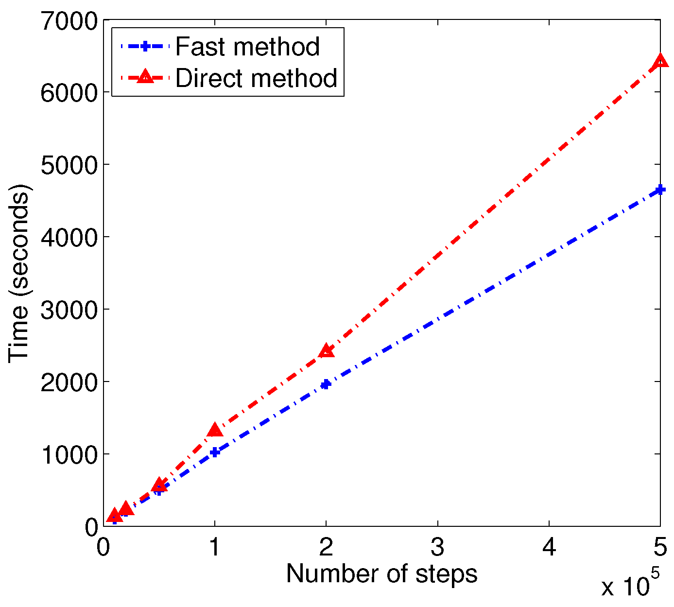
• The fast method is effective in reducing the computational time.
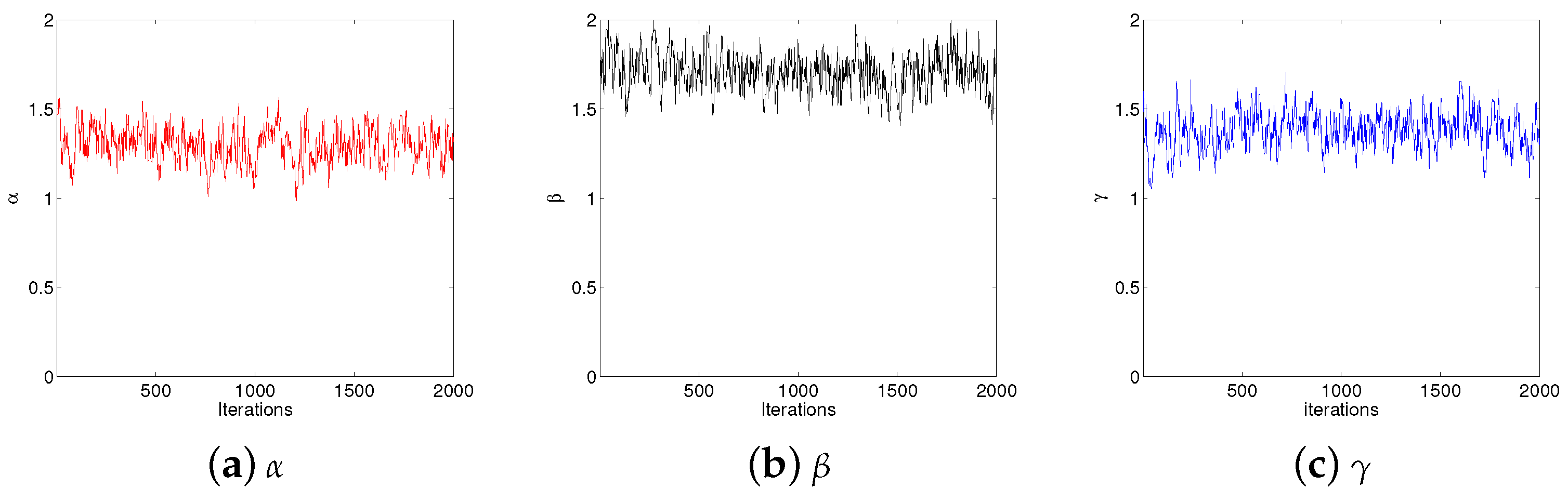
• Under different conditions, the parameter estimation method we propose can effectively estimate fractional derivative parameters and solve the problem of multi-parameter estimation in the coupled model.
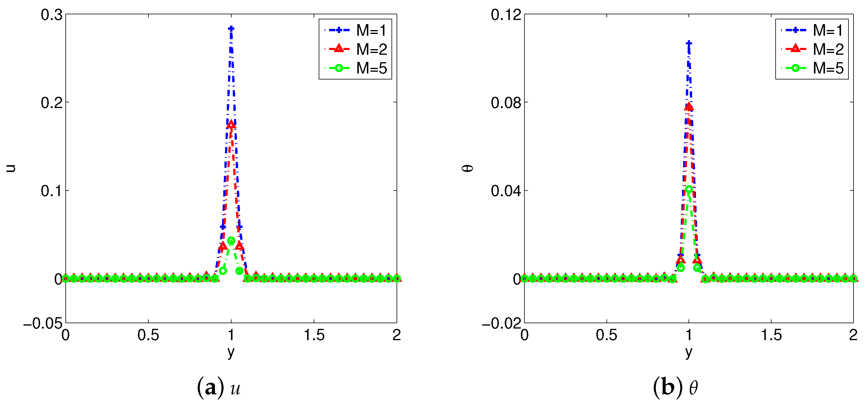
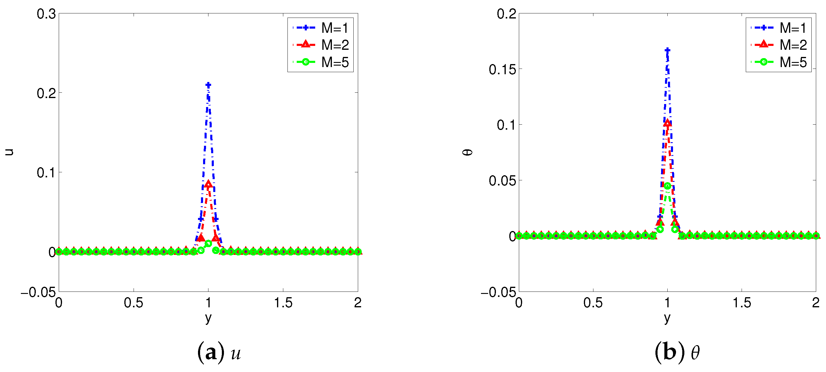
• The Lorentz force produced by the MHD flow will block the movement of the fluid and prolong the time for the fluid to reach a stable state. But the Hall parameter m will weaken this hindrance.
• The Joule heating effects play a negative role in heat transfer.
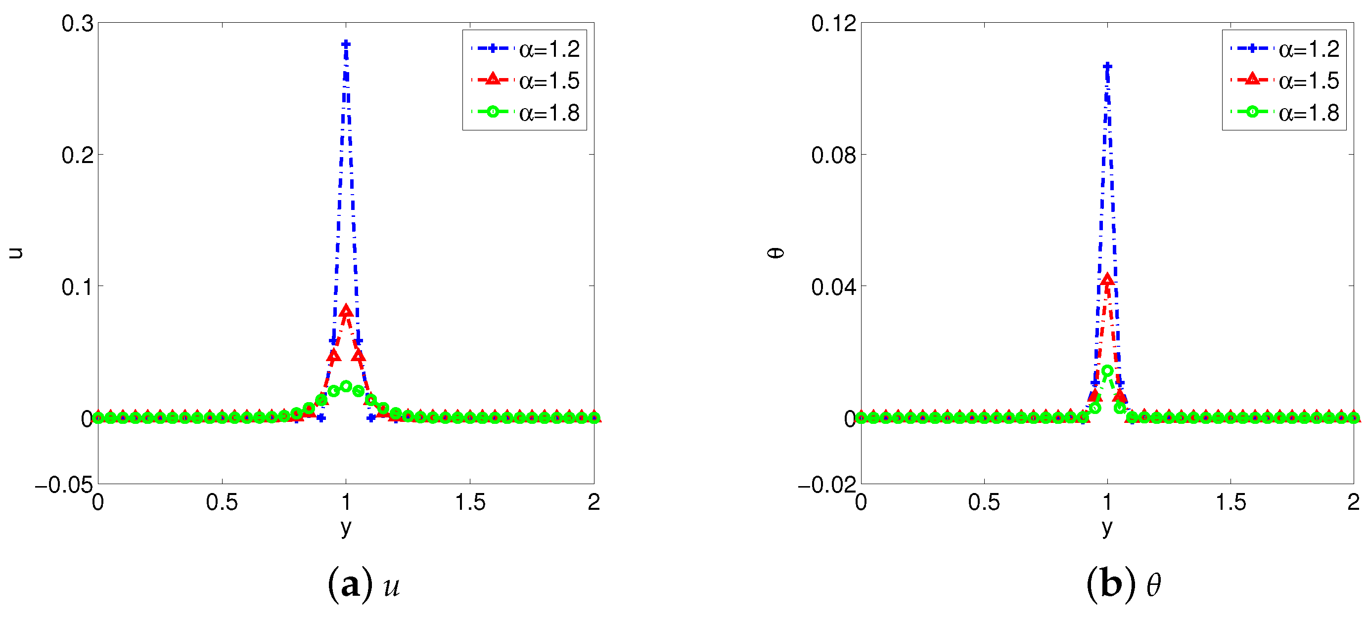
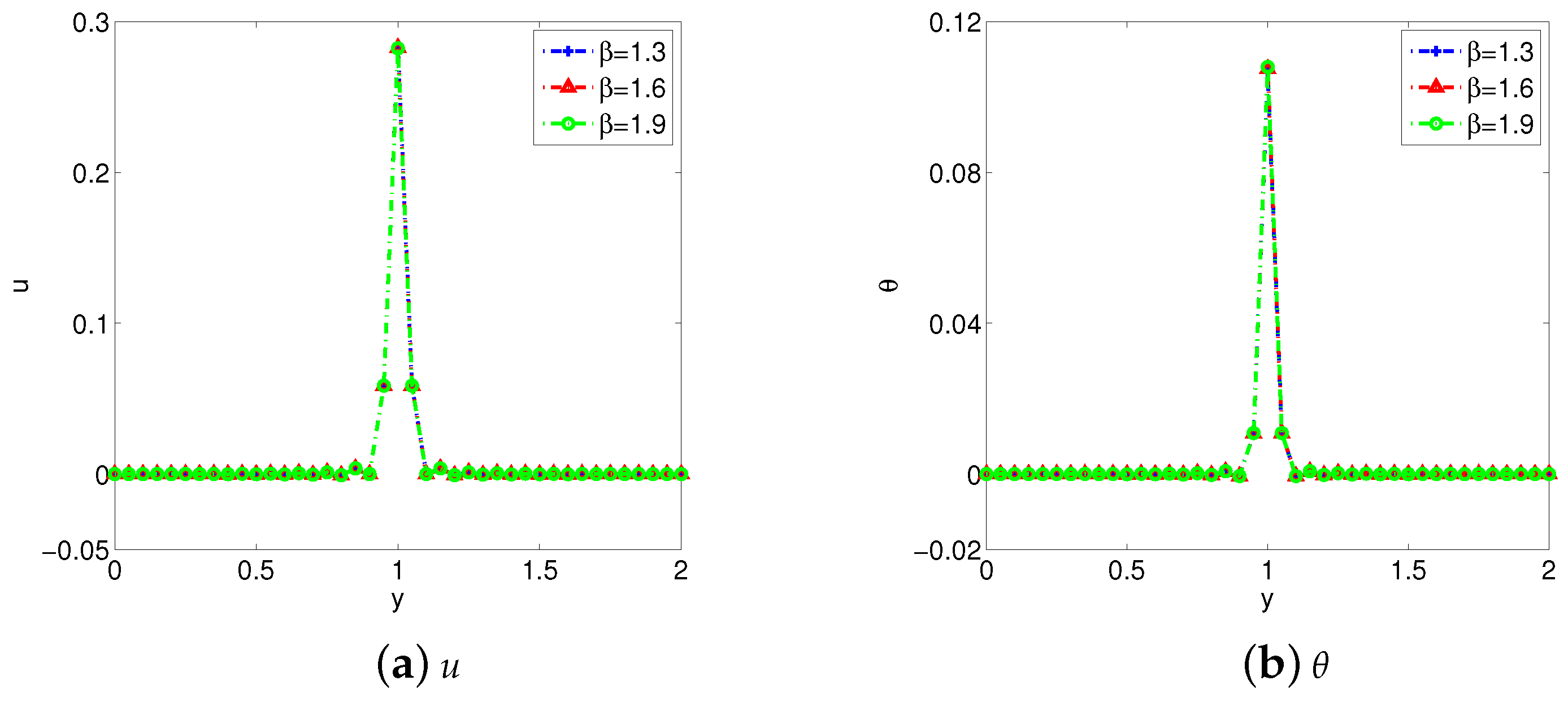
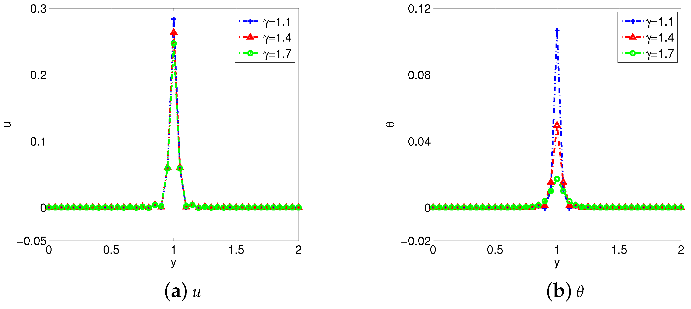
• Increasing the fractional derivative parameters $\alpha$, $\beta$, and $\gamma$ can promote the heat transfer, and make the flow become gentle in a short time.

Through the above results, the Lorentz force should be reduced by adjusting the magnitude of the magnetic field, simultaneously reducing the Joule heating effects, improving the fluid heat transfer speed and efficiency, and extending the service life of equipment. The numerical scheme and fast method in this paper make it possible to efficiently calculate the spatial fractional coupled model, and this work provides a method to estimate parameters, which makes the research on MHD flow and heat transfer more accurate. In further work, we shall investigate these methods in other high-dimensional fractional coupled problems to study more complex MHD flow and heat transfer processes, providing possibilities for improving production efficiency and reducing energy consumption.

References

- Zheng, R.; Guo, B. Global solutions to the ideal MHD system with a strong magnetic background. Nonlinear Anal. Real World Appl. 2021, 61, 103334. [Google Scholar] [CrossRef]
- Iftikhar, N.; Riaz, M.B.; Awrejcewicz, J.; Akgül, A. Effect of magnetic field with parabolic motion on fractional second grade fluid. Fractal Fract. 2021, 5, 163. [Google Scholar] [CrossRef]
- Madhura, K.; Atiwali, B.; Iyengar, S. Influence of nanoparticle shapes on natural convection flow with heat and mass transfer rates of nanofluids with fractional derivative. Math. Methods Appl. Sci. 2021, 46, 8089–8105. [Google Scholar] [CrossRef]
- Rehman, A.U.; Jarad, F.; Riaz, M.B.; Shah, Z.H. Generalized Mittag-Leffler Kernel form solutions of free convection heat and mass transfer flow of Maxwell fluid with Newtonian heating: Prabhakar fractional derivative approach. Fractal Fract. 2022, 6, 98. [Google Scholar] [CrossRef]
- Chen, X.; Yang, W.; Zhang, X.; Liu, F. Unsteady boundary layer flow of viscoelastic MHD fluid with a double fractional Maxwell model. Appl. Math. Lett. 2019, 95, 143–149. [Google Scholar] [CrossRef]
- Jiang, X.; Zhang, H.; Wang, S. Unsteady magnetohydrodynamic flow of generalized second grade fluid through porous medium with Hall effects on heat and mass transfer. Phys. Fluids 2020, 32, 113105. [Google Scholar] [CrossRef]
- Huang, Y.Y.; Gu, X.M.; Gong, Y.; Li, H.; Zhao, Y.L.; Carpentieri, B. A fast preconditioned semi-implicit difference scheme for strongly nonlinear space-fractional diffusion equations. Fractal Fract. 2021, 5, 230. [Google Scholar] [CrossRef]
- Kumar, D.; Nama, H.; Singh, J.; Kumar, J. An Efficient Numerical Scheme for Fractional Order Mathematical Model of Cytosolic Calcium Ion in Astrocytes. Fractal Fract. 2024, 8, 184. [Google Scholar] [CrossRef]
- Yang, Z.; Zeng, F. A corrected L1 method for a time-fractional subdiffusion equation. J. Sci. Comput. 2023, 95, 85. [Google Scholar] [CrossRef]
- Wang, X.; Qi, H.; Yang, X.; Xu, H. Analysis of the time-space fractional bioheat transfer equation for biological tissues during laser irradiation. Int. J. Heat Mass Transf. 2021, 177, 121555. [Google Scholar] [CrossRef]
- Jia, J.; Xu, H.; Jiang, X. Fast evaluation for the two-dimensional nonlinear coupled time–space fractional Klein-Gordon-Zakharov equations. Appl. Math. Lett. 2021, 118, 107148. [Google Scholar] [CrossRef]
- Jian, H.Y.; Huang, T.Z.; Ostermann, A.; Gu, X.M.; Zhao, Y.L. Fast numerical schemes for nonlinear space-fractional multidelay reaction-diffusion equations by implicit integration factor methods. Appl. Math. Comput. 2021, 408, 126360. [Google Scholar] [CrossRef]
- Koleva, M.N.; Vulkov, L.G. Parameters Estimation in a Time-Fractiona Parabolic System of Porous Media. Fractal Fract. 2023, 7, 443. [Google Scholar] [CrossRef]
- Zhang, H.; Jiang, X. Spectral method and Bayesian parameter estimation for the space fractional coupled nonlinear Schrödinger equations. Nonlinear Dyn. 2019, 95, 1599–1614. [Google Scholar] [CrossRef]
- Qin, H.; Li, L.; Li, Y.; Chen, X. Time-Stepping Error Estimates of Linearized Grünwald–Letnikov Difference Schemes for Strongly Nonlinear Time-Fractional Parabolic Problems. Fractal Fract. 2024, 8, 390. [Google Scholar] [CrossRef]
- Yang, X.; Liu, Y.; Park, G.K. Parameter estimation of uncertain differential equation with application to financial market. Chaos Solitons Fractals 2020, 139, 110026. [Google Scholar] [CrossRef]
- Yang, X.; Jiang, X.; Kang, J. Parameter identification for fractional fractal diffusion model based on experimental data. Chaos Interdiscip. J. Nonlinear Sci. 2019, 29, 083134. [Google Scholar] [CrossRef]
- Chi, X.; Yu, B.; Jiang, X. Parameter estimation for the time fractional heat conduction model based on experimental heat flux data. Appl. Math. Lett. 2020, 102, 106094. [Google Scholar] [CrossRef]
- Waini, I.; Ishak, A.; Pop, I. MHD flow and heat transfer of a hybrid nanofluid past a permeable stretching/shrinking wedge. Appl. Math. Mech. 2020, 41, 507–520. [Google Scholar] [CrossRef]
- Chi, X.; Zhang, H. Numerical study for the unsteady space fractional magnetohydrodynamic free convective flow and heat transfer with Hall effects. Appl. Math. Lett. 2021, 120, 107312. [Google Scholar] [CrossRef]
- Dai, M. Local well-posedness of the Hall-MHD system in Hs(n) with s > . Math. Nachrichten 2020, 293, 67–78. [Google Scholar] [CrossRef]
- Ghani, M. Local well-posedness of Boussinesq equations for MHD convection with fractional thermal diffusion in sobolev space Hs(n) × Hs+1−ϵ(n) × Hs+α−ϵ(n). Nonlinear Anal. Real World Appl. 2021, 62, 103355. [Google Scholar] [CrossRef]
- Xu, T.; Liu, F.; Lü, S.; Anh, V.V. Numerical approximation of 2D multi-term time and space fractional Bloch–Torrey equations involving the fractional Laplacian. J. Comput. Appl. Math. 2021, 393, 113519. [Google Scholar] [CrossRef]
- Farquhar, M.E.; Moroney, T.J.; Yang, Q.; Turner, I.W. GPU accelerated algorithms for computing matrix function vector products with applications to exponential integrators and fractional diffusion. SIAM J. Sci. Comput. 2016, 38, C127–C149. [Google Scholar] [CrossRef]
- Urschel, J.C. Uniform error estimates for the Lanczos method. SIAM J. Matrix Anal. Appl. 2021, 42, 1423–1450. [Google Scholar] [CrossRef]
- Jia, X.; Liang, X.; Shen, C.; Zhang, L.H. Solving the cubic regularization model by a nested restarting Lanczos method. SIAM J. Matrix Anal. Appl. 2022, 43, 812–839. [Google Scholar] [CrossRef]
- Zheng, R.; Jiang, X.; Zhang, H. Efficient and accurate spectral method for the time-fractional dual-phase-lag heat transfer model and its parameter estimation. Math. Methods Appl. Sci. 2020, 43, 2216–2232. [Google Scholar] [CrossRef]
- Li, Y.; Cao, G.; Wang, T.; Cui, Q.; Wang, B. A novel local region-based active contour model for image segmentation using Bayes theorem. Inform. Sci. 2020, 506, 443–456. [Google Scholar] [CrossRef]
- Demkowicz-Dobrzański, R.; Górecki, W.; Guţă, M. Multi-parameter estimation beyond quantum Fisher information. J. Phys. A Math. Theor. 2020, 53, 363001. [Google Scholar] [CrossRef]
- van de Schoot, R.; Depaoli, S.; King, R.; Kramer, B.; Märtens, K.; Tadesse, M.G.; Vannucci, M.; Gelman, A.; Veen, D.; Willemsen, J.; et al. Bayesian statistics and modelling. Nat. Rev. Methods Prim. 2021, 1, 1. [Google Scholar] [CrossRef]
Disclaimer/Publisher’s Note: The statements, opinions and data contained in all publications are solely those of the individual author(s) and contributor(s) and not of MDPI and/or the editor(s). MDPI and/or the editor(s) disclaim responsibility for any injury to people or property resulting from any ideas, methods, instructions or products referred to in the content. |
© 2024 by the authors. Licensee MDPI, Basel, Switzerland. This article is an open access article distributed under the terms and conditions of the Creative Commons Attribution (CC BY) license (https://creativecommons.org/licenses/by/4.0/).