Abstract
Considering that the degradation of ball screw grease involves fractal characteristics, which exhibit long-term dependency and autocorrelation, a multivariate accelerated degradation modeling and reliability assessment method based on the fractional Brownian motion process model is proposed in this paper. Firstly, a nonlinear accelerated degradation model of grease is established using fractional Brownian motion, considering the heterogeneity of samples as well as the memory effect and long-term dependence in the deterioration process, and realizing parameter estimation. Secondly, a multivariate reliability evaluation model is established by considering multivariate performance indicators in combination with the Frank copula function. Finally, the effectiveness and potential engineering application value of this method are verified through actual degradation data of the grease.
1. Introduction
Grease is known for its advantages of long life and high reliability, and grease stored for over 10 years will experience a reduction in life by 15% to 30% [1]. Grease has a long storage life, thus very little life data are available. However, product degradation data contain significant reliability information. Using degradation data to predict life has become an effective method for evaluating the lifespan of high-reliability products. Traditional methods of obtaining storage environment degradation data through on-site storage and laboratory simulation are resource-intensive and costly, making it difficult to collect sufficient data in a short time to evaluate grease storage reliability. Accelerated degradation test technology addresses this by applying stress levels higher than actual working conditions to the product, ensuring the consistency of the failure mechanism while significantly shortening the test cycle. By using accelerated degradation data and establishing a reliability evaluation model, the product life under actual working conditions can be extrapolated in a short period.
There are relatively few studies on assessing the storage life of grease. Most studies focus solely on exploring the aging behavior of grease under mechanical or thermal oxidative conditions. These studies typically examine a range of microscopic and macroscopic indicators such as micromorphology [2], rheological properties [3,4,5], friction properties [6,7], and oxidation properties [8,9]. However, the grease life is often not explicitly predicted. Moreover, due to the complex composition of grease and the varying lubrication requirements across different scenarios, multiple performance parameters are essential for characterization. These performance characterization parameters often exhibit interdependencies. Therefore, establishing a multivariate accelerated degradation reliability model for grease and accurately describing the relationships between performance parameters are crucial steps to ensure the precision of reliability modeling and evaluation.
Currently, reliability models based on performance degradation information are categorized into four types of assessment methods: failure physics models, degradation distribution models, degradation trajectory models, and random process models [10]. Among these, random process models describe the randomness of product degradation information, considering factors such as sample variations, time-varying uncertainty, and measurement uncertainties. Research on their application in degradation modeling continues to advance and undergo refinement. For instance, Hao et al. [11] introduced skew normal random effects to handle the non-normal behavior of degraded data. They proposed an extended inverse Gaussian process model, which overcame the limitations of the traditional inverse Gaussian model in perturbation measurements and improved the accuracy of fitting degraded data. Yu et al. [12] developed a generalized Wiener process model to address the randomness in real-time degradation data from online monitoring systems. They derived a closed-form approximate analytical solution for remaining life and evaluated model parameters using a recursive Bayesian filtering algorithm. Wang et al. [13] suggested a degradation model based on the generalized inverse Gaussian distribution to manage the heterogeneity observed in product performance within degradation data. They employed the Expectation–Maximization (EM) algorithm for parameter estimation and confirmed the efficacy of the proposed model in heterogeneous degradation modeling.
Considering that the degradation process of ball screw grease exhibits fractal characteristics such as long-term dependence and autocorrelations, fractional Brownian motion (FBM) is a type of random function exhibiting Gaussian random properties, initially proposed by Benoit B. Mandelbrot in 1968 [14]. FBM can effectively handle the fractal characteristics of grease degradation. Currently, FBM has performed well in the life prediction results of electromechanical and material fields such as roller bearings [15,16], Lithium-ion batteries [17,18], and composite materials [16,19].
From the standpoint of product degradation information, reliability models based on performance degradation can be categorized into univariate and multivariate coupled reliability models. The copula function is extensively applied in multivariate coupled degradation modeling, such as in complex electromechanical systems [20], metal materials [21,22], and composite materials [23]. The accelerated storage process test involves randomness, coupling, and uncertainty [24]. By integrating the copula function with the random Wiener process, the dependence structure among multiple performance characteristics can be effectively captured [25].
Therefore, this paper proposes a multivariate accelerated degradation modeling and reliability assessment method based on the FBM. The accelerated degradation model is constructed by using the FBM process model and the Arrhenius accelerated model. Taking into account multiple performance indicators, oil separation and cone penetration, the copula function is used to couple the cumulative failure marginal distribution density function of the degradation data from the two performance parameters into a joint distribution density function. Finally, the multivariate reliability evaluation model is established and extrapolated to determine the reliability level of the grease under natural storage conditions.
The remainder of the paper is organized as follows: Section 2 provides accelerated degradation modeling and parameter estimation method. Section 3 provides a copula function and reliability evaluation model. In Section 4, a set of actual accelerated storage tests of ball screws grease data is used to verify the effectiveness of the proposed method. Section 5 provides an overview of the content presented in this paper.
2. Accelerated Degradation Modeling Based on FBM
2.1. Fractional Brownian Motion
Fractional Brownian motion (FBM) is defined as a generalization of standard Brownian motion, which includes long-range dependence and self-similarity. The stochastic process BH(t) is constructed by convolving standard Brownian motion B(t) with a kernel function dependent on the Hurst exponent [14]. The integral form of FBM is as follows:
where BH(t) represents fractional Brownian motion, Γ(·) denotes the gamma function, and H is known as the Hurst exponent. The first integral represents the influence of the past on the process, and the second integral represents the accumulation of the current variations.
The autocorrelation function of the standard FBM is expressed as [26]:
Among them, t and s are two different moments in the FBM; H is an indicator used to determine whether the time series data follow a random walk or a partial random walk process. Different values of H exhibit distinct characteristics of the random process:
If 0 < H < 0.50, the increments of the process are negatively correlated.
If H = 0.5, the process follows a random walk, i.e., Brownian motion.
If 0.5 < H < 1, the increments of the process are positively correlated, indicating long-term dependence.
The R/S analysis method is used to calculate the Hurst exponent of a time series. This paper employs this method to calculate the value of H based on the grease degradation data. The specific steps are as follows:
- Divide the time series of length N into A subsets, each of length n = N/A, and calculate the mean value of each subset Ma, where a = 1, 2, …, A.
- In each subset, calculate the cumulative deviation of the first k points to the mean Ma and the range and standard deviation Sa of each subset, where Ni,a represent the i-th data point in the a-th subset.
- Calculate the re-standardized range .
- Increase the value of A and repeat the above steps to calculate (R/S)n over different time spans.
- Plot versus and calculate the value of H.
2.2. Degradation Model
The degradation data of cone penetration and oil separation indicate that the degradation process is nonlinear. Obtaining a closed expression for the probability density of life in a nonlinear diffusion process is challenging. Therefore, this paper converts nonlinear data into linear data using a time scale conversion function. The fractional Brownian motion with a time conversion function is expressed as [27]:
where X(t) is the degradation state of the model at time t, X(0) is the initial value, let X(0) = 0.
λ is the drift coefficient, representing the degradation rate of the model, and it follows a normal distribution λ~N(μλ, σλ); μλ is the mean value of the drift coefficient, representing the overall trend of the drift coefficient; σλ is the standard deviation of the drift coefficient, representing the fluctuation and uncertainty of the drift coefficient; Λ(t; θ) is a nonlinear function with θ as parameter, which represents the nonlinear characteristics of the model, let Λ(t; θ) = tθ; σH is the diffusion coefficient, which indicates the fluctuation degree of model degradation.
2.3. Acceleration Model
Accelerated stress has an impact on the drift coefficient mean μλ, drift coefficient standard deviation σλ. Therefore, in order to be closer to engineering practice and improve the accuracy of product reliability prediction, the above parameters need to be treated as functions of stress Sp. In accelerated degradation testing, temperature Sp was selected as the stress factor due to its accelerating effect on material degradation. As the temperature rises, the physical and chemical properties of lubricating grease, such as oxidation, thickener decomposition, and volatilization, change significantly, thereby speeding up the degradation process. Therefore, temperature stress is a key factor influencing the degradation rate of lubricating grease. According to the physical mechanism of grease failure under temperature stress, the Arrhenius model is selected [28]. Combined with the Arrhenius model, the functional expression of the relationship between each parameter and stress is given. To facilitate the solution of parameters, the logarithm of both sides of the Arrhenius model is taken, and the expression is as follows:
where
, A being a constant related to the intrinsic properties of the product;
, E being the activation energy of the lubricating grease; k is the thermodynamic Boltzmann constant; and
, T being the temperature in Kelvin.
The unknown parameters in the nonlinear Wiener accelerated degradation model of lubricating grease are expressed as a function of the temperature stress Sp:
where the parameters aλ, bλ, cλ and dλ represent the sensitivity of the drift coefficient and its variability to changes in temperature stress. These parameters are fitted through empirical models, reflecting the degradation behavior of lubricating grease under different temperature stresses.
2.4. Parameter Estimation
Assume that the parameter
is to be estimated in the FBM model. The historical observation value is
, where m is the number of historical data. Since Equation (3) describes the degradation over time, the degraded observation value at the k-th instance can be expressed as follows:
where X(0) = 0.
Among them,
is a set of degradation observations. Combining
forms observation vector Y. Y satisfies the multidimensional distribution,
; the FBM model vector is
, and its covariance matrix can be expressed as:
Let
, then the mean and covariance matrix of Y can be obtained as:
The joint probability density distribution function of Y is then as follows:
To ensure the optimal solution, a log-likelihood function of the joint probability density distribution function based on Elastic Net Regularization [29] is proposed as follows:
where
,
,
, κ is the regularization parameter,
is the weight controlling the two regularization terms,
is the L1 norm of the parameter
, and
is the L2 norm of the parameter
.
To calculate the maximum likelihood estimates for μλ and σλ, let
Substituting Equations (13) and (14) into the log-likelihood function Equation (11), the conditional log-likelihood function is obtained:
To efficiently solve model parameters and obtain an accurate global optimal solution, this study introduces the manta ray foraging optimization algorithm to estimate parameter
. The algorithm uses Tent chaotic mapping to optimize the diversity of the initial population. Based on the characteristic of the Sigmoid function, where the function value increases as the x-coordinate moves away from the origin, the Sigmoid function is introduced into chain search and spiral foraging to accelerate the convergence speed of inferior solutions toward the optimal solution. Additionally, the differential evolution algorithm is employed to optimize the individual position update strategy during the somersault foraging phase, significantly reducing the probability of getting trapped in local optima.
3. Multivariate Reliability Assessment Model
3.1. Copula Function
The copula function can determine the joint probability distribution from the marginal probability distributions of random variables, thereby describing the degree of correlation between two random variables. In this paper, the degradation data of two characteristic indicators, cone penetration and oil separation of grease, are fitted to determine their marginal distributions. The distribution density image features are then compared with those of commonly used binary copula functions to preliminarily select the closest copula functions. Finally, the degree of fit is tested using the rank correlation coefficient and information criteria to select the optimal copula function.
The rank correlation coefficient and information equation are presented in Table 1. The square Euclidean distance represents the degree of fit between each copula function and the empirical copula function; a smaller value indicates a better fit. The Akaike Information Criterion (AIC), based on the entropy maximization principle in information theory, measures model complexity and goodness of fit. It is suitable for models that evaluate unknown parameters using the Maximum Likelihood Estimation (MLE). A smaller AIC value indicates a better predictive fit.

Table 1.
Rank correlation coefficient and information equation.
Where
; * represents various types of copula functions;
is the overall log-likelihood function; and
is the number of unknown parameters. In each copula model, ρ represents the dependency parameter, which is used to control the strength and direction of the association between variables. In Clayton and Gumbel copula, ρ takes positive values, and the larger the value, the stronger the tail dependence. For Gaussian copula, ρ ranges from −1 to 1, indicating a linear correlation between variables. For Frank copula, ρ can take any real value, and the larger the value, the stronger the dependence.
3.2. Reliability Assessment Model
For non-monotonic random degradation process models, the product life is usually defined as the first hitting time (FHT) when the random degradation process attenuation curve reaches the failure threshold. So the pre-failure time Lk at time tk is expressed as follows:
where lk is the length after tk time, and w is the failure threshold.
Based on FHT and weak convergence theory, the FBM model can be approximated by the dynamic diffusion coefficient as follows:
where
,
is the Gamma function, and
in the expression of the Brownian motion
and
in the fractional Brownian motion process have the same distribution at time t.
Let
, then Equation (6) can be written as:
Based on the uncertainty of the drift coefficient λ in parameter estimation, the probability density function (PDF) is expressed as follows:
where
,
,
,
.
This paper studies the case with two performance degradation quantities. Each performance degradation quantity is described by a Wiener random process with time scale transformation.
represents the degradation quantity of the ith performance parameter under accelerated stress
. Then, the binary nonlinear FBM can be expressed as follows:
where i = 1, 2, i = 1 represents the cone penetration change rate (CPCR), i = 2 represents the oil permeability change rate (OPCR), and p = 1, 2, 3, 4 represents the stress level number.
According to Equation (20), the distribution function of the natural storage reliability life of grease considering sample differences is obtained:
where
,
,
,
, and Φ(x) represents the cumulative distribution function (CDF) of the standard normal distribution.
The reliability function of the coupling of the two performance parameters is obtained by combining the copula distribution function
where
represents the copula linear correlation coefficient under conventional storage stress (25 °C).
is the corresponding copula distribution function.
If the Frank copula is chosen as the link function, the corresponding
is
If the Gaussian copula is chosen as the link function, the corresponding
is
4. Case Study
This case uses OPCR and CPCR data as the degradation data of grease to build a multivariate accelerated degradation model and conduct a reliability assessment. In this section, copula function selection, parameter estimation of the multivariate accelerated degradation model, and comparative reliability assessments of multiple models will be sequentially carried out.
4.1. Experiment Method
The research focuses on a specific brand of wide-temperature-range grease designed for long-term storage and heavy-load ball screw pairs. All test greases were manufactured by the same producer on the same date and passed factory inspection, meeting quality standards. The study examines the long-term storage environment of heavy-duty ball screw pairs with a 3.5 mm ball diameter. A grease storage test fixture was developed to increase grease storage capacity and reduce sampling costs while maintaining consistent storage conditions. The specific structure is depicted in Figure 1. To simulate high-temperature conditions, the study employs the grease reliability storage test platform, which is the existing environmental stress accelerated aging test device(THV-600-A, Suzhou Sushi Testing Instrument Co., Ltd., Suzhou, China), as shown in Figure 2. This platform allows accelerated reliability testing of various lubricants under different temperature and humidity conditions. The combination of the storage test platform and fixture enables assessment of aging performance and prediction of grease lifespan.
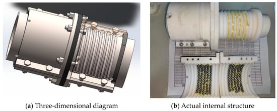
Figure 1.
Grease test fixture.
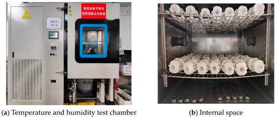
Figure 2.
Grease aging test system.
An intelligent optimization algorithm is employed to solve the optimal solution for the optimization design model of the grease storage accelerated degradation test scheme. This paper specifies a total of six samples at each stress level, with each sample being tested 15 times at equal intervals throughout the test cycle. The test scheme and sampling cycle are detailed in Table 2.

Table 2.
Experimental protocol.
4.1.1. Performance Indicators and Measurement Methods
The oil penetration ability of grease is crucial during normal operation. Grease can be likened to a porous sponge structure [30], where a thickener forms the sponge-like structure to retain base oil and release it under shear or extreme pressure, ensuring effective lubrication for frictional contact [31,32]. The oil penetration process of the base oil usually takes place in a form of micro-flow that conforms to Darcy’s law [33]. During prolonged storage aging, the internal structure of grease may deteriorate, leading to a decrease in oil penetration rate that renders the grease unusable.
The SKF MaPro test method (TKGT1, SKF, Sweden), which uses blotting paper to observe the oil area, offers higher accuracy and is suitable for small quantities of grease [34]. In this method, a specified volume of grease is placed within a defined circle S0, and after uniform heating at a prescribed temperature and time, the grease is heated through oil penetration to area S1, as shown in Figure 3. The grease penetration rate is quantified by the size of area S1; a larger S1 represents a greater penetration rate.
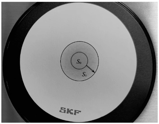
Figure 3.
SKF MaPro test method.
Cone penetration measurement can reflect grease consistency and has the advantage of being detected simply and at low cost. Grease with a smaller cone entry value will exhibit greater consistency and, accordingly, can withstand larger loads. Grease with a larger cone entry has a reduced load-carrying capacity but benefits from easier addition and less resistance to movement. The cone entry degree of grease should fall within a specific interval; if it is too large or too small, it will have a negative effect on grease performance. Influenced by mechanical aging or high-temperature aging, the thickener breaks down, leading to an increase in the cone penetration value of the grease [35,36]. Most of the current grease cone penetration measurements are performed using cone penetration instruments, and these measurements are primarily based on the ASTM standards D217 and D1403 [37]. In this paper, a 1/4 cone penetration measurement(HSY-269D, Shanghai Qigao Instrument Co., Ltd., Shanghai, China) was selected for measurement based on the actual grease storage capacity of the tooling.
4.1.2. Data Preprocessing
To maintain consistency in the degradation order of magnitude, dimensions, and degradation trends of oil separation and cone penetration, normalization processing is conducted. The OPCR of the grease is chosen as the indicator of oil permeability, as shown in the following formula:
where S1 is the oil separation area of fresh grease, Si is the oil separation area of grease after aging, and S0 is the area of the grease itself. The degradation state of the test samples is continuously monitored, and the grease test is stopped when the degradation state exceeds the failure threshold three consecutive times.
The CPCR is selected as the cone penetration index, as shown in the following formula:
where
represents the original 1/4 cone penetration of the grease,
represents the 1/4 cone penetration of the grease after degradation, and
represents the normalized 1/4 cone penetration of the grease after degradation. An increase in
indicates a decrease in the 1/4 cone penetration of the degraded grease
, implying that the penetration has decreased and the grease has become thicker.
Based on the test results of cone penetration and oil separation degree of the lubricating grease subjected to accelerated degradation tests, the original scatter plot of degradation data is shown in Figure 4. It can be observed that as the stress level increases and degradation time progresses, the cone penetration of the grease decreases, while the area of diffusion speckles increases, indicating a reduction in oil separation degree. There is a positive correlation between oil separation degree and cone penetration.
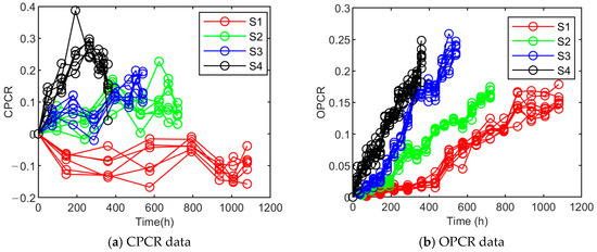
Figure 4.
Grease degradation data.
The R/S method is used to verify the Hurst index of the grease accelerated storage degradation data, as shown in Table 3. The Hurst index of both sets of data is
. Therefore, the data sets used are all consistent with the FBM model with long-term dependence.

Table 3.
Hurst index of the grease accelerated storage degradation data.
4.2. Copula Function Selection
The frequency distribution histogram of cone penetration and oil separation is plotted based on the degradation data, as shown in Figure 5. Through the normality test, it is observed that the cone penetration degradation data generally follow a normal distribution, while the overall distribution type of the oil separation degradation data is difficult to determine. Therefore, the non-parametric method of kernel density is used to determine the overall distribution, with the respective empirical distribution functions and kernel distributions shown in Figure 6. Figure 7 presents the bivariate frequency distribution histogram of cone penetration and oil separation degree, where variable U represents CPCR and variable V represents OPCR. Figure 7a shows the frequency count, which indicates the actual number of observations of the combination of bivariate U and V. In contrast, Figure 7b shows the normalized frequency, which indicates the relative frequency of these combinations. It is observed that both characteristic parameters exhibit sharp peaks and thick tails, and the tails are roughly symmetrical. Thus, the binary Gaussian copula function and the binary Frank copula function are selected to describe the correlation characteristics of the performance index parameters.
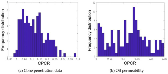
Figure 5.
Frequency distribution histogram of degradation data.
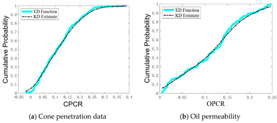
Figure 6.
Empirical distribution function and kernel density.
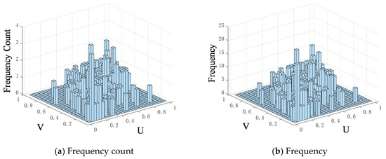
Figure 7.
Bivariate distribution histogram.
Based on the equations in Table 1, The linear correlation coefficients of the binary Gaussian copula and binary Frank copula functions were estimated, and both coefficients were positive, indicating a positive correlation in the data. The probability density function and distribution function images of the binary Gaussian copula and binary Frank copula were plotted, as shown in Figure 8 and Figure 9. Compared to the binary Gaussian copula function, the binary Frank copula function has a thicker tail, which aligns more closely with the binary frequency distribution histogram shown in Figure 7b and better reflects the tail correlation between the variables. Consequently, the binary Frank copula function was initially selected to describe the characteristics of the two variables. As shown in Table 4, the Pearson linear correlation coefficient, Kendall rank correlation coefficient, and Spearman rank correlation coefficient were calculated. The analysis indicates that, compared to the binary Gaussian copula function, the Kendall and Spearman rank correlation coefficients of the binary Frank copula function are closer to those directly derived from the original observation data of the two performance parameters. Additionally, the square Euclidean distance is smaller, and the AIC information criterion is lower. Therefore, under the dual criteria of square Euclidean distance and Akaike information criterion, the binary Frank copula function, with a linear correlation parameter of 5.9517, provides a better fit for the observed data of cone penetration and oil separation. Thus, from a fitting prediction perspective, the binary Frank copula function is selected to describe the characteristics of the two variables. The empirical copula distribution function is drawn as shown in Figure 10, closely matching the results fitted by these two copula functions.
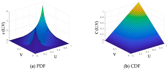
Figure 8.
Bivariate normal copula function.
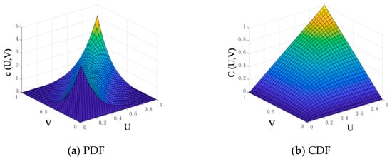
Figure 9.
Bivariate Frank copula function.

Table 4.
Rank correlation coefficient and information content.
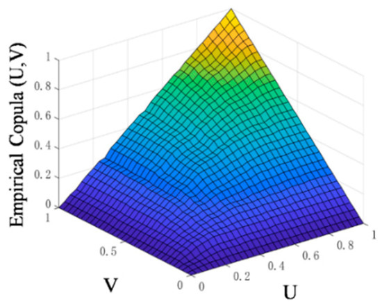
Figure 10.
Empirical copula distribution function.
4.3. Natural Storage Equivalent Life Assessment
Based on Equations (5)–(14) in parameter estimation, the estimated values of model parameters under the CPCR and OPCR degradation data are shown in Table 5. The regularization coefficients were determined as κ = 0.07 and α = 0.15 by adjusting the AIC value.

Table 5.
Degradation model parameter regression estimates.
The failure thresholds of CPCR and OPCR are 0.52 and 0.5, respectively. When the values are exceeded, the grease is considered to be failed [38]. Substituting the grease temperature (fixed at 25 °C) under natural storage conditions in the warehouse into Equation (4), and substituting the relevant parameters and performance failure thresholds into Equations (21)–(24), the reliability under each normal temperature storage stress state is obtained. The median life of the grease during natural storage, when
, is predicted as shown in Table 6.

Table 6.
Natural storage reliability median life and AIC.
4.4. Comparision with Other Models
The estimated model parameters and the performance failure thresholds were substituted into the reliability calculation formula to obtain the following reliability functions: the reliability function considering only the single performance parameter of cone penetration, the reliability function considering only the single performance parameter of oil permeability, the reliability function considering the independent dual performance parameters of cone penetration and oil permeability, the reliability function not considering sample differences, and the reliability function considering the Frank correlation of dual performance parameters of cone penetration and oil separation degree with sample differences, as shown in Figure 11a. The corresponding life probability density function curves are shown in Figure 11b.
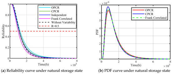
Figure 11.
Reliability assessment under natural storage state.
Based on the estimated results of lubricating grease at room temperature storage, various scenarios show different median life predictions: considering only cone penetration yields approximately 13.88 years, while focusing solely on oil permeability gives about 13 years. When considering both cone penetration and oil permeability independently, the median life is around 12.63 years. Without accounting for sample differences, the median life estimate is approximately 13.04 years. Incorporating the Frank correlation between cone penetration and oil permeability, with sample differences considered, results in a median life prediction of approximately 11.31 years.
This analysis reveals varying reliability under different performance indicators. The reliability life predicted using cone penetration is longer than that using oil permeability, suggesting a slower degradation rate for cone penetration. However, relying solely on cone penetration to assess grease life may miss failures when oil permeability exceeds its threshold. Predicting reliability using dual performance parameters results in a shorter life expectancy compared to single parameters, indicating reduced prediction risk. The median life considering the Frank correlation of cone penetration and oil permeability with sample differences in this section is more conservative than when considering independent dual parameters. This approach ensures that grease failure is not overlooked when either parameter reaches its failure threshold first.
5. Conclusions
In view of the limited storage reliability and life data of ball screw grease, and the fractal characteristics of the degradation process, such as long-term correlation and autocorrelation, this paper proposes a multivariate accelerated degradation modeling and reliability assessment based on the fractional Brownian motion process model. First, the nonlinear accelerated degradation model of grease is established by using the FBM process model, considering the heterogeneity of samples, memory effect and long-term correlation in the degradation process, and realizing parameter estimation. Secondly, the multivariate performance index is considered in combination with the Frank copula function. Then, a multivariate reliability function model is established to realize reliability assessment. Finally, the case analysis data are obtained from the accelerated storage test of ball screw grease, and the oil separation and cone penetration of the grease are selected as performance indicators for reliability assessment. The median reliability life of the grease under actual storage conditions is calculated by the proposed model to be about 11.31 years. By comparing with the single performance index model or other copula function models, the proposed multivariate degradation reliability model has lower prediction risk and more accurate results. This method is expected to be applied to the storage life assessment of various types of grease products in the future, and has important theoretical and engineering value.
Author Contributions
Conceptualization, C.C.; Methodology, C.C., Z.L. and J.Z.; Formal analysis, C.W.; Investigation, C.W. and P.C.; Data curation, C.W.; Writing—original draft, C.C. and C.W.; Writing—review & editing, C.C., Z.L. and J.G.; Supervision, J.G. and P.C.; Funding acquisition, C.C., Z.L. and J.G. All authors have read and agreed to the published version of the manuscript.
Funding
This research was funded by National Natural Science Foundation of China (Grant number 52305537, U23B20104, and U22B2087), Key Scientific and Technological Research Project of Jilin Province (Grant number 20230201104GX), Natural Science Foundation of Chongqing Municipality (Grant No. cstc2021jcyj-msxmX0935 and No. CSTB2022NSCQ-MSX0902), Jilin Provincial Department of Education Scientific Research Project (Grant number JJKH20231155KJ).
Data Availability Statement
Data are contained within the article.
Conflicts of Interest
The authors declare that they have no known competing financial interests or personal relationships that could have appeared to influence the work reported in this paper.
References
- Krakhmalev, S.I.; Shkol’nikov, V.M.; Platonova, R.G. Effect of a change in the properties of plastic grease in storage in a container and in an article on the reliability of operation of friction units. Chem. Technol. Fuels Oils 2010, 46, 319–327. [Google Scholar] [CrossRef]
- Lin, C.-L.; Meehan, P.A. Microstructure Characterization of Degraded Grease in Axle Roller Bearings. Tribol. Trans. 2019, 62, 667–687. [Google Scholar] [CrossRef]
- Zheng, J.; Li, Y.; Wang, J.; Shiju, E.; Li, X. Accelerated thermal aging of grease-based magnetorheological fluids and their lifetime prediction. Mater. Res. Express 2018, 5, 085702. [Google Scholar] [CrossRef]
- Zakani, B.; Ansari, M.; Grecov, D. Dynamic rheological properties of a fumed silica grease. Rheol. Acta 2018, 57, 83–94. [Google Scholar] [CrossRef]
- Gonçalves, D.; Graça, B.; Campos, A.V.; Seabra, J.; Leckner, J.; Westbroek, R. Formulation, rheology and thermal ageing of polymer greases—Part I: Influence of the thickener content. Tribol. Int. 2015, 87, 160–170. [Google Scholar] [CrossRef]
- Pan, J.; Cheng, Y.; Yang, J. Effect of heat treatment on the lubricating properties of lithium lubricating grease. RSC Adv. 2015, 5, 58686–58693. [Google Scholar] [CrossRef]
- Wu, C.; Xiong, R.; Ni, J.; Yao, L.; Chen, L.; Li, X. Effects of CuO nanoparticles on friction and vibration behaviors of grease on rolling bearing. Tribol. Int. 2020, 152, 106552. [Google Scholar] [CrossRef]
- Li, L.; Liu, J.J.; Tian, Z.Y.; Zhang, G.Z.; Fu, Z.Y.; Li, T. Ageing Evaluation of No.2 Lithium Lubricating Grease. Adv. Mater. Res. 2013, 763, 121–124. [Google Scholar] [CrossRef]
- Huang, L.; Guo, D.; Cann, P.M.; Wan, G.T.Y.; Wen, S. Thermal Oxidation Mechanism of Polyalphaolefin Greases with Lithium Soap and Diurea Thickeners: Effects of the Thickener. Tribol. Trans. 2016, 59, 801–809. [Google Scholar] [CrossRef]
- Wang, F.; Xiao, Y.; Cui, P.; Lin, J.; Li, M.; Chen, Z. Correlation of asphalt performance indicators and aging Degrees: A review. Constr. Build. Mater. 2020, 250, 118824. [Google Scholar] [CrossRef]
- Hao, S.; Yang, J.; Berenguer, C. Degradation analysis based on an extended inverse Gaussian process model with skew-normal random effects and measurement errors. Reliab. Eng. Syst. Saf. 2019, 189, 261–270. [Google Scholar] [CrossRef]
- Yu, W.; Shao, Y.; Xu, J.; Mechefske, C. An adaptive and generalized Wiener process model with a recursive filtering algorithm for remaining useful life estimation. Reliab. Eng. Syst. Saf. 2022, 217, 108099. [Google Scholar] [CrossRef]
- Wang, Z.; Zhai, Q.; Chen, P. Degradation modeling considering unit-to-unit heterogeneity-A general model and comparative study. Reliab. Eng. Syst. Saf. 2021, 216, 107897. [Google Scholar] [CrossRef]
- Mandelbrot, B.B.; Van Ness, J.W. Fractional Brownian Motions, Fractional Noises and Applications. SIAM Rev. 1968, 10, 422–437. [Google Scholar] [CrossRef]
- Song, W.; Zhong, M.; Yang, M.; Qi, D.; Spadini, S.; Cattani, P.; Villecco, F. Remaining Useful Life Prediction of Roller Bearings Based on Fractional Brownian Motion. Fractal Fract. 2024, 8, 183. [Google Scholar] [CrossRef]
- Zhang, H.; Zhou, D.; Chen, M.; Xi, X. Predicting remaining useful life based on a generalized degradation with fractional Brownian motion. Mech. Syst. Signal Process. 2019, 115, 736–752. [Google Scholar] [CrossRef]
- Wang, H.; Song, W.; Zio, E.; Kudreyko, A.; Zhang, Y. Remaining useful life prediction for Lithium-ion batteries using fractional Brownian motion and Fruit-fly Optimization Algorithm. Measurement 2020, 161, 107904. [Google Scholar] [CrossRef]
- Zhang, H.; Mo, Z.; Wang, J.; Miao, Q. Nonlinear-Drifted Fractional Brownian Motion With Multiple Hidden State Variables for Remaining Useful Life Prediction of Lithium-Ion Batteries. IEEE Trans. Reliab. 2020, 69, 768–780. [Google Scholar] [CrossRef]
- Yan, S.; Liang, Y. A fractal model for characterizing multi-scaling particle diffusion behaviors in alkali-activated materials system. Cem. Concr. Res. 2024, 175, 107386. [Google Scholar] [CrossRef]
- Zhou, H.; Parlikad, A.K.; Brintrup, A.; Harrison, A. A copula-based quantified airworthiness modelling for civil aircraft engines. Probabilistic Eng. Mech. 2023, 73, 103481. [Google Scholar] [CrossRef]
- Xiao, R.; Zayed, T.; Meguid, M.; Sushama, L. Time varying reliability analysis of corroded gas pipelines using copula and importance sampling. Ocean Eng. 2024, 306, 118086. [Google Scholar] [CrossRef]
- Barros, B.; Conde, B.; Riveiro, B.; Morales-Nápoles, O. Gaussian Copula-based Bayesian network approach for characterizing spatial variability in aging steel bridges. Struct. Saf. 2024, 106, 102403. [Google Scholar] [CrossRef]
- Van Bavel, B.; Vandepitte, D.; Moens, D. Vine copulas for accelerated prediction of composite strength variability. Comput. Struct. 2024, 301, 107440. [Google Scholar] [CrossRef]
- Chen, R.; Zhang, C.; Wang, S.; Zio, E.; Dui, H.; Zhang, Y. Importance measures for critical components in complex system based on Copula Hierarchical Bayesian Network. Reliab. Eng. Syst. Saf. 2023, 230, 108883. [Google Scholar] [CrossRef]
- Sun, F.; Fu, F.; Liao, H.; Xu, D. Analysis of multivariate dependent accelerated degradation data using a random-effect general Wiener process and D-vine Copula. Reliab. Eng. Syst. Saf. 2020, 204, 107168. [Google Scholar] [CrossRef]
- Sottinen, T. Fractional Brownian motion, random walks and binary market models. Financ. Stoch. 2001, 5, 343–355. [Google Scholar] [CrossRef]
- Asgari, A.; Si, W.; Yuan, L.; Krishnan, K.; Wei, W. Multivariable degradation modeling and life prediction using multivariate fractional Brownian motion. Reliab. Eng. Syst. Saf. 2024, 248, 110146. [Google Scholar] [CrossRef]
- Lugt, P.M. On the use of the Arrhenius equation to describe the impact of temperature on grease life. Tribol. Int. 2023, 179, 108142. [Google Scholar] [CrossRef]
- Wang, X.; Wang, P.; Song, Y.; Xiang, Q.; Li, J. Recognition of high-resolution range profile sequence based on TCN with sequence length-adaptive algorithm and elastic net regularization. Expert Syst. Appl. 2024, 248, 123417. [Google Scholar] [CrossRef]
- Zhang, Q.; Mugele, F.; Lugt, P.M.; van den Ende, D. Characterizing the fluid–matrix affinity in an organogel from the growth dynamics of oil stains on blotting paper. Soft Matter 2020, 16, 4200–4209. [Google Scholar] [CrossRef] [PubMed]
- Saatchi, A.; Shiller, P.J.; Eghtesadi, S.A.; Liu, T.; Doll, G.L. A fundamental study of oil release mechanism in soap and non-soap thickened greases. Tribol. Int. 2017, 110, 333–340. [Google Scholar] [CrossRef]
- Salomonsson, L.; Stang, G.; Zhmud, B. Oil/thickener interactions and rheology of lubricating greases. Tribol. Trans. 2007, 50, 302–309. [Google Scholar] [CrossRef]
- Akchurun, A.; Ende, D.V.D.; Lugt, P.M. Modeling impact of grease mechanical ageing on bleed and permeability in rolling bearings. Tribol. Int. 2022, 170, 107507. [Google Scholar] [CrossRef]
- Noordover, A.; David, S.; Fiddelaers, F.; Van Den Kommer, A. Grease Test Kit and Methods of Testing Grease. Google Patents US9341611B2, 17 May 2016. [Google Scholar]
- Lee, C.-H.; Choi, J.Y.; Jeon, I.S.; Cho, W.; Yun, H. Grease Degradation in Constant Velocity (CV) Joints. Tribol. Trans. 2011, 54, 825–831. [Google Scholar] [CrossRef]
- Rezasoltani, A.; Khonsari, M. On the correlation between mechanical degradation of lubricating grease and entropy. Tribol. Lett. 2014, 56, 197–204. [Google Scholar] [CrossRef]
- ASTMD217-19b; Standard Test Methods for Cone Penetration of Lubricating Grease. ASTM International: West Conshohocken, PA, USA, 2019.
- Lugt, P.M. Grease Lubrication in Rolling Bearings; John Wiley & Sons: Hoboken, NJ, USA, 2012. [Google Scholar]
Disclaimer/Publisher’s Note: The statements, opinions and data contained in all publications are solely those of the individual author(s) and contributor(s) and not of MDPI and/or the editor(s). MDPI and/or the editor(s) disclaim responsibility for any injury to people or property resulting from any ideas, methods, instructions or products referred to in the content. |
© 2024 by the authors. Licensee MDPI, Basel, Switzerland. This article is an open access article distributed under the terms and conditions of the Creative Commons Attribution (CC BY) license (https://creativecommons.org/licenses/by/4.0/).