Parameters Estimation in a Time-Fractiona Parabolic System of Porous Media

Abstract

The simultaneous estimation of coefficients and the initial conditions for model fractional parabolic systems of porous media is reduced to the minimization of a least-squares cost functional. This inverse problem uses information about the pressures at a finite number of space time points. The Frechet gradient of the cost functional is derived. The application of the conjugate gradient method for numerical parameter estimation is also discussed. Computational results with noise-free and noisy data illustrate the efficiency and accuracy of the proposed algorithm.

1. Introduction

Many industrial, environmental, and biological processes, related to solute transport in porous media and groundwater, see, e.g., [1,2,3], are modeled using a dispersion-reaction system of equations. The solving of such parabolic systems of equations of heterogeneous porous media usually requires the application of numerical methods.

Recently, there has been a sharp increase in research activities on modeling the flow of fluids in porous media with complex pore networks.

Complex processes in the fractional porous media require some type of model reduction, see, e.g., [4,5,6,7,8].

Many time-fractional diffusion equations and diffusion wave equations appear when the integer time derivatives are replaced by the fractional derivatives, and this technology is also used in porous media modeling. However, apart from such formal action, similar equations describe large classes of physical and chemical processes, such as anomalous diffusion, turbulent flow, chaotic dynamics, etc. A remarkable consequence of turbulence is the emergence of anomalous diffusion, see, e.g., [9].

We wrote the system of equations for flow in the triple continuum approach (4) in [8]. The first continuum describes a flow in the matrix of the porous media, the second continuum belongs to the network of a small highly connected fractured network, and the third continuum is related to the flow in a low-dimensional fractured network. We have the following system of equations for $\mathbf{p}=(p_1,p_2,p_f)$:

$$C_1\frac{{\partial }^{{\alpha }_1}{p}_1}{\partial t^{{\alpha }_1}}-\nabla .(k_1\nabla p_1)={\eta }_{12}(p_2-p_1)+{\eta }_{1f}(p_f-p_1),\mathsf{\Omega }\times (0,T),$$

(1)

$$C_2\frac{{\partial }^{{\alpha }_2}{p}_2}{\partial t^{{\alpha }_2}}-\nabla .(k_2\nabla p_2)={\eta }_{21}(p_1-p_2)+{\eta }_{2f}(p_f-p_2),\mathsf{\Omega }\times (0,T),$$

(2)

$$C_f\frac{{\partial }^{{\alpha }_f}{p}_f}{\partial t^{{\alpha }_f}}-\nabla .(k_f\nabla p_f)={\eta }_{f1}(p_1-p_f)+{\eta }_{f2}(p_2-p_f),\mathsf{\Gamma }\times (0,T),$$

(3)

where $\mathsf{\Omega }\subset R^d$, $\mathsf{\Gamma }\in R^{d-1}$ and for the continuum index $i=1,2,f$, $\mathbf{p}$ denotes the pressure, $k_i$ is the permeability, $k_i\ge k_{i0}>0$, $i=1,2$, $k_f\ge 0$, and ${\eta }_{is}$ is the mass transfer term, which are proportional to the continuum permeabilities. The left time Caputo derivative [10,11,12,13] is used:

$$\frac{d^{\alpha }u\left(t\right)}{d{t}^{\alpha }}=\frac{1}{\mathsf{\Gamma }(1-\alpha )}{\int }_0^t{(t-\lambda )}^{-\alpha }\frac{du\left(\lambda \right)}{d\lambda }d\lambda ,0<\alpha <1,\alpha ={\alpha }_1,{\alpha }_2,{\alpha }_f.$$

for the function $p_i(x,t)$, $i=1,2,f$.

All further results can easily be extended to the model for multi-continuum media:

$$C_i\frac{{\partial }^{{\alpha }_i}{p}_i}{\partial t^{{\alpha }_i}}-\nabla .(k_i\nabla p_i)=\sum _{s\ne i}^I{\eta }_{is}(p_s-p_i)+{\eta }_{if}(p_f-p_i),\mathsf{\Omega }\times (0,T),$$

(4)

where $i=1,\dots ,I$ and I is the number of contaminants.

The numerical method, based on the implicit finite difference approximation for the time approximation and the generalized multiscale finite element method for the spatial discretization is developed in [8] for solving the systems (1)–(4), $k_f=0$.

The one-dimensional case of the same model is studied in [14,15]. A priori estimates for the solutions of the first and third boundary value problems of the system (1)–(3), using energy inequalities, are obtained in [14]. In [15] is the constructed and analyzed positivity preserving numerical method for solving the second and third boundary value problems of the system (1)–(3). For the temporal discretization, the $L1$ formula on the non-uniform mesh is utilized while, for the discretization in space, a second-order monotone discretization on half-integer grid nodes is used.

The inverse problems, where it is required to determine some of the coefficients in the differential equations, initial values, boundary values, and some of the fractional orders ${\alpha }_1,\dots ,{\alpha }_I,{\alpha }_f$ by the observation data of solution $\mathbf{p}=(p_1,\dots ,p_I,p_f)$, are important.

The inverse problem is indispensable for the precise and accurate modeling for analyzing many phenomena, such as heat-mass transfer, atmospheric pollution, and porous media, see, e.g., [5,9,10,16,17]. After relevant investigations of inverse problems, we can identify coefficients, boundary conditions, etc., to determine the equations themselves and can step into solving initial boundary value problems and initial value problems. Therefore, the inverse problem is the premise for studying the corresponding forward problem.

In the last decades, many research works indicated that the fractional differential equations are more relevant than those of classical models to describe non-Darcian flow or anomalous diffusion in some especial environment, in particular porous media, see, e.g., [18,19,20].

Actually, the aim of the current work is not only to establish a theory for direct problems related to time-fractional differential equations, but, first of all, to apply the theory to inverse problems. The inverse problems are highly various and, in this paper, we consider one inverse problem to illustrate how our framework for fractional derivative models operates. However, for inverse problems for the time-fractional diffusion equations, and especially for the systems of such equations, for example, to recover the initial data, source function, or diffusion coefficient, and so on, with some additional information, there are not so many works, see, e.g., [9,21,22,23,24,25] and references therein. Even fewer are the results for simultaneously identifying more parameters in fractional order systems.

The rest of this paper is structured as follows. In the next section, we introduce some preliminaries concerning the fractional order calculus. We discuss the well-posedness of the direct (forward) problem in the one-dimensional case in Section 3. We also present some a priori estimates for the solution. Inverse problems are formulated in Section 4, while the quasi-solution of one of these problems is discussed in Section 5. The gradient of the cost functional is derived in the next section. The conjugate gradient method (CGM) is described in Section 7. The finite difference method (FDM) for the numerical solution of the inverse problem is presented in Section 8. The results from the numerical experiments are proposed and discussed in Section 9. The paper is finalized with some conclusions.

2. Preliminaries

In this section, we introduce useful notation and some formulas from fractional calculus without the precision of the smoothness of the functions, see, e.g., [12,13,26] for more details.

We consider another classical fractional derivative called the left Riemann–Liouville derivative:

$$D_0^{\alpha }u\left(t\right)=\frac{1}{\mathsf{\Gamma }(1-\alpha )}\frac{d}{dt}{\int }_0^t{(t-\lambda )}^{-\alpha }u\left(\lambda \right)d\lambda ,0<t<T,$$

while

$$\left(I^{\alpha }u\right)\left(t\right)=D_t^{-\alpha }u\left(t\right)=\frac{1}{\mathsf{\Gamma }\left(\alpha \right)}{\int }_0^t{(t-\lambda )}^{\alpha -1}u\left(\lambda \right)d\lambda$$

is the left Riemann–Liouville integral of order $\alpha$. Next, the right Riemann–Liouville integral and derivative are defined:

$$\left(I_{\alpha }u\right)\left(t\right)=D_T^{-\alpha }u\left(t\right)=\frac{1}{\mathsf{\Gamma }\left(\alpha \right)}{\int }_t^T{(\lambda -t)}^{\alpha -1}u\left(\lambda \right)d\lambda ,$$

$$D_T^{\alpha }u\left(t\right)=\frac{-1}{\mathsf{\Gamma }(1-\alpha )}\frac{d}{dt}{\int }_t^T{(\lambda -t)}^{-\alpha }u\left(\lambda \right)d\lambda ,$$

We also use the integration-by-parts formula:

$${\int }_0^T\frac{{\partial }^{\alpha }u}{\partial t^{\alpha }}v\left(t\right)dt-{\int }_0^{T}u\left(t\right)D_T^{\alpha }v\left(t\right)dt=u\left(T\right)D_T^{-\alpha }v\left(T\right)-u\left(0\right)D_T^{-\alpha }v\left(0\right).$$

(5)

The relationship between the Caputo and Rieamann–Liouville derivatives is given as follows:

$$\frac{d_0^{\alpha }u\left(t\right)}{d{t}^{\alpha }}=D_0^{\alpha }u\left(t\right)-\frac{u\left(0\right)}{\mathsf{\Gamma }(1-\alpha )}{t}^{-\alpha },t\in (0,T],$$

(6)

$$\frac{d_T^{\alpha }u\left(t\right)}{d{t}^{\alpha }}=D_T^{\alpha }u\left(t\right)-\frac{u\left(T\right)}{\mathsf{\Gamma }(1-\alpha )}{(T-t)}^{-\alpha },t\in [0,T),$$

where

$$\frac{d_T^{\alpha }u\left(t\right)}{d{t}^{\alpha }}=-\frac{1}{\mathsf{\Gamma }(1-\alpha )}{\int }_t^T{(\lambda -t)}^{-\alpha }\frac{du\left(\lambda \right)}{d\lambda }d\lambda ,$$

is the right Caputo derivative.

Further, we will use one- and two-parameter Mittag-Leffler functions [12,13]:

$$\begin{array}{c}\hfill E_{{\beta }_1,{\beta }_2}\left(z\right)=\sum _{s=0}^{\infty }\frac{z^s}{\mathsf{\Gamma }({\beta }_{1}s+{\beta }_2)},E_{\beta }\left(z\right)=E_{\beta ,1}\left(z\right)=\sum _{s=0}^{\infty }\frac{z^s}{\mathsf{\Gamma }(\beta s+1)}.\end{array}$$

(7)

3. The Direct Problem

In this section, we introduce a model parabolic system (direct problem) with first or third boundary conditions and present two theorems that are useful for the following investigations.

Without the loss of generality, and for simplicity, in this paper, we develop our approach for the particular case of system (1)–(4), the triple continuum model in [27], in 1D geometry, as well as the models in [18,19,20]. Namely, in the rectangle ${\overline{Q}}_T=\{(x,t):0\le x\le 1,$ $0\le t\le T\}$, we consider the first boundary value problem:

$$\begin{array}{c}{C}_1\frac{{\partial }^{{\alpha }_1}{p}_1}{\partial t^{{\alpha }_1}}=\frac{\partial }{\partial x}\left(k_1(x,t)\frac{\partial p_1}{\partial x}\right)-{\eta }_{12}(x,t)(p_1-p_2)-{\eta }_{1f}(x,t)(p_1-p_f)+g_1(x,t),\hfill \end{array}$$

(8)

$$\begin{array}{c}{C}_2\frac{{\partial }^{{\alpha }_2}{p}_2}{\partial t^{{\alpha }_2}}=\frac{\partial }{\partial x}\left(k_2(x,t)\frac{\partial p_2}{\partial x}\right)-{\eta }_{21}(x,t)(p_2-p_1)-{\eta }_{2f}(x,t)(p_2-p_f)+g_2(x,t),\hfill \end{array}$$

(9)

$$\begin{array}{c}{C}_f\frac{{\partial }^{{\alpha }_f}{p}_f}{\partial t^{{\alpha }_f}}=\frac{\partial }{\partial x}\left(k_f(x,t)\frac{\partial p_f}{\partial x}\right)-{\eta }_{f1}(x,t)(p_f-p_1)-{\eta }_{f2}(x,t)(p_f-p_2)+g_f(x,t),\hfill \end{array}$$

(10)

$$\begin{array}{c}{p}_i(0,t)=0,p_i(1,t)=0,0<t\le T,i=1,2,f,\hfill \end{array}$$

(11)

$$\begin{array}{c}{p}_i(x,0)={\phi }_i\left(x\right),x\in \mathsf{\Omega }=(0,1),i=1,2,f.\hfill \end{array}$$

(12)

The existence and uniqueness of a weak solution to the initial boundary value problem (8)–(12) could be investigated following the scheme developed in [4]. Then, the stronger regularity of the weak solution of the direct problem (8)–(11) for more smooth input data can be established as well. Throughout the following, we assume that there exists a solution:

$$\mathbf{p}(x,t)\equiv (p_1(x,t),p_2(x,t),p_f(x,t))\in C^{2,1}({\overline{Q}}_T,)$$

of the problem (3), (4), and (8)–(11), where $C^{m,n}\left({\overline{Q}}_T\right)$ is the class of the functions that, together with their partial derivatives of order m with respect to x and order n with respect to t, are continuous in ${\overline{Q}}_T=\overline{\mathsf{\Omega }}\times [0,T]$. Therefore, throughout this paper we are interested in the classical solutions of (8)–(12), i.e., functions $\mathbf{p}=(p_1,p_2,p_3)$ whose derivatives $\frac{{\partial }^{{\alpha }_i}{p}_i}{\partial t^{{\alpha }_i}}$, $i=1,2,f$, and $\frac{{\partial }^2{p}_i}{\partial x^2},$ exist at all points in Q and satisfy (8)–(12) pointwise.

The following results, obtained in [14], will be used in the quasi-solution and the analysis of the sensitivity problem in Section 5 and Section 6.

Theorem 1.

If $k_i(x,t)\in C^{1,0}\left({\overline{Q}}_T\right)$, $i=1,2,f$, ${\eta }_{is}\in C\left({\overline{Q}}_T\right)$, $i,s=1,2,f$, $g_i(x,t)\in C\left({\overline{Q}}_T\right),k_i(x,t)\ge k_{i0}>0$, $i=1,2$, $k_f\ge 0$, and ${\mu }_{is}\ge {\eta }_{is}(x,t)\ge 0,s=1,2,f$ everywhere in ${\overline{Q}}_T$. Then, the initial-value problem (8)–(12) has a unique classical solution that satisfies the a priori estimate:

$$\begin{array}{ccc}& & E\left(t\right)\le E\left(0\right)E_{\beta }(\rho ,t^{\beta })+\mathsf{\Gamma }\left(\beta \right)E_{\beta ,\beta }\left({\rho }_1{t}^{\beta }\right)D_{0t}^{-\beta }{\rho }_2\left(t\right),\beta =min({\alpha }_1,{\alpha }_2,{\alpha }_f),\hfill \\ & & E\left(t\right)=\sum _{i=1}^2{\int }_{\mathsf{\Omega }}{C}_i^2{p}_i^2\left(x\right)dx+{\int }_{\mathsf{\Omega }}{C}_f{p}_f^2(x,t)dx,\hfill \\ & & {\rho }_2\left(t\right)=\sum _{i=1}^2{\int }_{\mathsf{\Omega }}{g}_i^2(x,t)dx+{\int }_{\mathsf{\Omega }}{g}_f^2(x,t)dx,\hfill \end{array}$$

(13)

where ${\rho }_1$ is a constant and $E_{\beta },E_{\beta ,\beta }$ are Mittag-Leffler functions (7).

For the proof, see the conference paper (Theorem 1 in [14]) and Appendix A.

In the problem (8)–(12), we replace the boundary conditions (11) in the following way:

$$\begin{array}{c}\hfill \begin{array}{cc}\hfill & k_i(0,t)\frac{\partial p_i(0,t)}{\partial x}={\beta }_{1i}\left(t\right)p_i(0,t)-{\mu }_{1i}\left(t\right),i=1,2,0<t\le T,\hfill \\ \hfill -& k_i(1,t)\frac{\partial p_i(1,t)}{\partial x}={\beta }_{2i}\left(t\right)p_i(1,t)-{\mu }_{2i}\left(t\right),i=1,2,0<t\le T.\hfill \end{array}\end{array}$$

(14)

In the rectangle ${\overline{Q}}_T$, we consider the third boundary value problem (8), (10), (12), and (14).

Theorem 2.

If, in addition to the assumptions of Theorem 1,

$${\beta }_{1i}\left(t\right),{\beta }_{2i}\left(t\right),{\mu }_{1i}\left(t\right),{\mu }_{2i}\left(t\right)\in C[0,T],\parallel {\beta }_{1i}\left(t\right)\parallel \le b_1,\parallel {\beta }_{2i}\left(t\right)\parallel \le b_2,b_i,i=1,2,$$

are constants, for all $t\in [0,T]$ values, then the solution $\mathbf{p}(x,t)\equiv (p_1(x,t),p_2(x,t),p_f(x,t))$ of the problems (8), (10), (12), and (14) satisfies the a priori estimate:

$$\begin{array}{c}\hfill \begin{array}{cc}\hfill & \sum _{i=1}^2\parallel C_i^{1/2}{p}_i{\parallel }_0^2+{\parallel C_f^{1/2}{p}_f\parallel }_0^2+D_{0t}^{-\beta }\left(\sum _{i=1}^2{∥C_i^{1/2}\frac{\partial p_i}{\partial x}∥}_0^2+{∥C_f^{1/2}\frac{\partial p_f}{\partial x}∥}_0^2\right)\hfill \\ & \le M(D_{0t}^{-\beta }\left(\sum _{i=1}^2\parallel g_i^2{\parallel }_0^2+\parallel g_f^2{\parallel }_0+\sum _{i,s=1}^2{D}_{0t}^{-\beta }{\mu }_{is}^2\left(t\right)+\sum _{i=1}^2\parallel {\phi }_i{\parallel }_0^2+{\parallel {\phi }_f\parallel }_0^2\right)\hfill \end{array}\end{array}$$

For the proof, see the conference paper (Theorem 2 in [14]) and Appendix A.

The proofs of Theorems 1 and 2 are based on the ideas in paper [28].

4. The Inverse Problems

In the fractional models, there are parameters, e.g., diffusion and convection, reaction coefficients, or boundary conditions, as well as initial conditions, and source terms that are difficult for observation purposes and have to be inferred indirectly from measurements. This gives rise to many different fractional differential equation inverse problems.

More precisely, we study the inverse problem (IP) of the identification of the permeability-fluid viscosity constant coefficients $k\equiv \{k_1,\dots ,k_I,k_f\}$, the mass transfer coefficients $\eta \equiv \{{\eta }_{is}(x,t),{\eta }_{if}(x,t),i,s=1,\dots ,I,f\}$, and the initial conditions $\phi \left(x\right)\equiv \{{\phi }_1\left(x\right)=p_1(x,0),\dots ,{\phi }_I\left(x\right)=p_I(x,0),{\phi }_f\left(x\right)=p_f(x,0)\},$ if additional information can be measured:

$${\mathit{p}}_i(x_l,t_m;a)=G_{lm}^i,l=1,\dots ,L,m=1,\dots ,M$$

(15)

and $i\in \widehat{I}\le \{1,\dots ,I,f\},a=\{\eta ,k,\phi \}\in A$, where A is the admissible set.

It can be rewritten in the operator form $\mathcal{A}\left(a\right)=g$, where $\mathcal{A}:A\to G$ is an injective operator and $a\in A,g\in G$ is an Euclidean space of data $g=\{G_{11}^i,\dots ,G_{LM}^i\}$. The inverse problem $\mathcal{A}\left(a\right)=g$ is ill-posed, i.e., its solution may not exist and/or its solution is non-unique and/or unstable to errors in measurements (15), see, e.g., [9,12,16,26,29].

Since the unknowns may not be uniquely identified due to the limited amount of inversion output, the inverse problem is often reformulated as an optimization problem with the minimizers considered as the approximate solution in some general sense. Here, the inverse problem is reduced to the minimization problem:

$$a=argminJ\left(a\right),J\left(a\right)=\frac{1}{2}〈\mathcal{A}\left(a\right)-g,\mathcal{A}\left(a\right)-g〉,$$

where the functional $J\left(a\right)$ characterizes the quadratic deviation of the model data from the experimental data, and we take it as follows:

$$J\left(a\right)=\sum _{i\in \widehat{I}}\sum _{l=1}^L\sum _{m=1}^M{(p_i(x_l,t_m;a)-G_{lm}^i)}^2.$$

(16)

Of course, there are many other problems, which may be formulated for the determination of the coefficients, the right-hand side of the differential equations, or the initial conditions, for example:

IP1 the reconstruction of the coefficients $k_1(x,t),\dots ,k_I(x,t)$ and $k_f(x,t)$ from the pressure measurements at several time moments $0<t_1<\cdots <t_m\le T$;

IP2 the reconstruction of the initial pressure ${\phi }_i\left(x\right)$ from the final time observation $p_i(x,T)$;

IP3 the simultaneous reconstruction of the mass transfer coefficients ${\eta }_{is}(x,t)$ and the initial pressure ${\phi }_i\left(x\right)$ at the above measurements;

IP4 the simultaneous reconstruction of the permeability $k_1(x,t),\dots ,k_I(x,t)$ and $k_f(x,t)$ with the transfer coefficients ${\eta }_{is}(x,t)$.

5. Quasi-Solution of the Inverse Problem IP

This section is devoted to the formulation and existence of a quasi-solution to the IP.

Further, we concentrate on the IP and, for more clarity, we will consider the triple continuum model (8)–(12), where $d=1$, $I=2$, $k_1$, $k_2$ are positive constants, and $k_f$ is a non-negative constant, as well as ${\eta }_{12}={\eta }_{21}=e\left(t\right)$, ${\eta }_{1f}={\eta }_{f1}=b\left(t\right)$, ${\eta }_{2f}={\eta }_{f2}=c\left(t\right)$, i.e., we have three mass transfer coefficients. Additionally, we will take $C_1=C_2=C_f=1$.

Let us precise the admissible set:

$$A=\{a:0<k_1,k_2<K,0\le k_f<K_f,0\le e\left(t\right),b\left(t\right),c\left(t\right)\in L^2(0,T),\phi \in {\left(L^2\left(\mathsf{\Omega }\right)\right)}^3\}.$$

We rewrite the functional $J\left(a\right)$ as follows:

$$J\left(a\right)=\sum _{i\in \widehat{I}}\sum _{l=1}^L\sum _{m=1}^M{\int }_0^T{\int }_{\mathsf{\Omega }}{(p_i(x,t;a)-G_{lm}^i)}^2\delta (x-x_l)\delta (t-t_m)dxdt,$$

(17)

where $\delta (·)$ is the Dirac-delta function, reformulating the inverse problem as a minimization problem for the functional $J\left(a\right)$, namely:

$$J\left(\overline{a}\right)=\underset{a\in A}{min}J\left(a\right).$$

If $\hat{a}\in A$, such that $J\left(\hat{a}\right)=0$, then the solution of the minimization problem (15) is called the exact solution of the inverse coefficient problem IP. Otherwise, the solution of the minimization problem is called the quasi-solution, see, e.g., [24,27,28,29].

Theorem 3.

A minimizer $a^{*}=arg{min}_{a\in A}J\left(a\right),$ exists.

The proof follows the arguments as in (Chapter 6 in [24]), so we omit them.

6. The Gradient of the Cost Functional $\mathit{J}\mathbf{\left(}\mathit{a}\mathbf{\right)}$

In this section, we analyze the sensitivity problem and then derive the Frechet derivative of the functional (16).

Now, we can introduce the matrices with the vector $\eta =(e,b,c)$ and the following matrices:

$$B=\left(b_{i\nu }\right)=\left(\begin{array}{ccc}-e-b& e& b\hfill \\ e& -e-c& c\hfill \\ b& c& -b-c\hfill \end{array}\right),$$

$$Q=\left(q_{i\nu }\right)=\left(\begin{array}{ccc}-p_1+p_2& -p_1+p_f& 0\\ -p_2+p_1& 0& -p_2+p_f\\ 0& -p_f+p_1& -p_f+p_2\end{array}\right).$$

Next, if $\delta a$ is an increment, we denote the deviation of solution $\mathbf{p}(p_1,p_2,p_f)$ by $\delta \mathbf{p}(x,t;\delta a)=\mathbf{p}(x,t;a+\delta a)-\mathbf{p}(x,t;a)$. Then, if it satisfies the following initial boundary value problem with accuracy up to terms of order $o\left(\right|\delta a{|}^2)$, the sensitivity problem is as follows:

$$\begin{array}{c}\hfill \begin{array}{cc}\hfill & L_1\delta p_1=\frac{{\partial }^{{\alpha }_1}\delta p_1}{\partial t^{{\alpha }_1}}-k_1\frac{{\partial }^2\delta p_1}{\partial x^2}-\sum _{\nu =1}^{\mathcal{V}}{b}_{1\nu }\delta p_{\nu }-\sum _{s=1}^S{q}_{1s}\delta {\eta }_s-\delta k_1\frac{{\partial }^2{p}_1}{\partial x^2}=0,\hfill \\ & L_2\delta p_2=\frac{{\partial }^{{\alpha }_2}\delta p_2}{\partial t^{{\alpha }_2}}-k_2\frac{{\partial }^2\delta p_2}{\partial x^2}-\sum _{\nu =1}^{\mathcal{V}}{b}_{2\nu }\delta p_{\nu }-\sum _{s=1}^S{q}_{2s}\delta {\eta }_s-\delta k_2\frac{{\partial }^2{p}_2}{\partial x^2}=0,\hfill \\ & L_3\delta p_3=\frac{{\partial }^{{\alpha }_f}\delta p_f}{\partial t^{{\alpha }_f}}-k_f\frac{{\partial }^2\delta p_f}{\partial x^2}-\sum _{\nu =1}^{\mathcal{V}}{b}_{3\nu }\delta p_{\nu }-\sum _{s=1}^S{q}_{3s}\delta {\eta }_s-\delta k_f\frac{{\partial }^2{p}_f}{\partial x^2}=0,\hfill \\ & \mathcal{V}=I+1=2+1=3,S=3,p_3=p_f.\hfill \\ & {\left.\delta p_i\right|}_{x=0}={\left.\delta p_i\right|}_{x=1}=0,i=1,2,f,\hfill \\ & \delta p_i(x,0)=\delta {\phi }_i\left(x\right),x\in \mathsf{\Omega }=(0,1),i=1,2,f,t\in (0,T).\hfill \end{array}\end{array}$$

(18)

Lemma 1.

The mapping $a\mapsto p\left(a\right)$ is Lipschitz continuous from A to $H^{1,0}\left(Q_T\right)$, i.e., for any $a+\delta a\in A$, the solution $\mathbf{p}\in H^{1,0}\left(Q_T\right)$ to the problem (8)–(12) satisfies:

$$\parallel \delta \mathbf{p}\left(a\right)\parallel ={\parallel \mathbf{p}(a+\delta a)-\mathbf{p}\left(a\right)\parallel }_{H^{1,0}\left(Q_T\right)}\le c{\parallel \delta a\parallel }_{L^{\infty }\left(\mathsf{\Omega }\right)}.$$

(19)

Proof. 

The increment $\delta p$ is a solution of the sensitivity problem (16). Next, we follow similar arguments as in Theorem 1 to obtain the estimate (18). □

We have considered the first boundary value problem (8)–(12). In a similar way, we can derive the sensitivity problem when third boundary conditions (14) are posed. Then, the corresponding boundary conditions take the form:

$$\begin{array}{ccc}\hfill & & k_i\frac{\partial \delta p_i}{\partial x}+\delta k_i\frac{\partial p_i}{\partial x}={\beta }_{1i}\left(t\right)\delta p_i\mathrm{for}x=0,\hfill \\ \hfill & & -\left(k_i\frac{\partial p_i}{\partial x}+\delta k_i{p}_i\right)={\beta }_{2i}\left(t\right)\delta p_i\mathrm{for}x=1.\hfill \end{array}$$

On the basis of Theorem 2, one can obtain an estimate analogously to (19). □

Now, we are in a position to formulate our main result.

Theorem 4.

The gradient of the cost functional $J\left(a\right)$ is given by the following:

$$J^{\prime }\left(a\right)={\left({\int }_{\mathsf{\Omega }}{Q}^{T_r}R(x,t)dx,{\int }_{\mathsf{\Omega }}{\int }_0^T\frac{{\partial }^2{\mathbf{p}}^{T_r}}{\partial x^2}(x,t)\circ R(x,t)dtdx,R(x,0)\right)}^{T_r},$$

(20)

where ∘ is the Hadamard product and the vector function $R(x,t)$ is the solution of the adjoint problem ($\mathcal{V}=3$):

$$\begin{array}{c}\hfill \begin{array}{cc}\hfill & D_T^{{\alpha }_1}{r}_1=k_1\frac{{\partial }^2{r}_1}{\partial x^2}-\sum _{\nu =1}^{\mathcal{V}}{b}_{\nu 1}{r}_{\nu }+S_1,\hfill \\ & D_T^{{\alpha }_2}{r}_2=k_2\frac{{\partial }^2{r}_2}{\partial x^2}-\sum _{\nu =1}^{\mathcal{V}}{b}_{\nu 2}{r}_{\nu }+S_2,\hfill \\ & D_T^{{\alpha }_f}{r}_f=k_f\frac{{\partial }^2{r}_f}{\partial x^2}-\sum _{\nu =1}^{\mathcal{V}}{b}_{\nu 3}{r}_{\nu }+S_3,\mathcal{V}=I+1=3,r_3=r_f,\hfill \\ & r_i(x,T)=0,x\in \mathsf{\Omega },{\left.r_i\right|}_{x=0}={\left.r_i\right|}_{x=1}=0,i=1,2,f,\hfill \\ & S_i=\sum _{m=1}^M\sum _{l=1}^L{\int }_0^T{\int }_{\mathsf{\Omega }}{(p_i(x,t;a)-G_{lm}^i)}^2\delta (t-t_m)\delta (x-x_l)dxdt,\hfill \end{array}\end{array}$$

(21)

for $i=1,2,f$, $p_3=p_f$, and $\delta (t-t_m)$ is the Dirac-delta function.

Proof. 

The proof is performed in two parts:

Part 1. For the increment of the cost functional (17), we have:

$$\begin{array}{c}\hfill \begin{array}{cc}\hfill \delta J& =J(a+\delta a)-J\left(a\right)=\sum _{l=1}^L\sum _{m=1}^M{\left(\delta p(x_l,t_m;\delta a)\right)}^2\hfill \\ & +\sum _{l=1}^L\sum _{m=1}^M{\int }_0^l(p(x,t;a)-G_{lm})\delta p(x,t;a)\delta (x-x_l)\delta (t-t_k).\hfill \end{array}\end{array}$$

(22)

Part 2. We write the variational formulation of the sensitivity problem (18) using $R(x,t)$ as a test function.

We organize the scalar product $\langle ·,·\rangle$ in $Q_T$ of the system (18) with the vector $R(x,t)\equiv (r_1(x,t),r_2(x,t),r_f(x,t))$ and by its components, meaning we have:

$$\begin{array}{c}\hfill \begin{array}{cc}\hfill 〈L_i\delta p_i,{\mathsf{\Psi }}_i〉=& {\int }_0^T{\int }_0^l\frac{{\partial }^{{\alpha }_i}\delta p_i}{\partial t^{{\alpha }_i}}{\mathsf{\Psi }}_{i}dxdt-k_1{\int }_0^T{\int }_0^l\frac{{\partial }^2\delta p_i}{\partial x^2}{\mathsf{\Psi }}_{i}dxdt\hfill \\ & -\sum _{i=1}^{\mathcal{V}}{\int }_0^T{\int }_0^l{b}_{i\nu }\delta p_{\nu }{\mathsf{\Psi }}_{i}dxdt-\sum _{s=1}^S{\int }_0^T{\int }_0^L{q}_{1s}\partial {\eta }_s{\mathsf{\Psi }}_{i}dxdt\hfill \\ & -\delta k_i{\int }_0^T{\int }_0^l\frac{{\partial }^2{p}_i}{\partial x^2}{\mathsf{\Psi }}_{i}dxdt,i=1,2,f,\delta k_f=0.\hfill \end{array}\end{array}$$

Now, we perform integration by parts (5), using the boundary and initial conditions in (18) and (21). For example, with respect to the first equation of (18), we have:

$$\begin{array}{ccc}& & 〈\frac{{\partial }^{{\alpha }_1}\delta p_1}{\partial t^{{\alpha }_1}},r_1〉={\int }_0^l{\int }_0^T\frac{{\partial }^{{\alpha }_1}\delta p_1}{\partial t^{{\alpha }_1}}{r}_{1}dtdx=〈\delta p_1,D_T^{{\alpha }_1}{r}_1〉,\hfill \\ & & k_1〈\frac{{\partial }^2\delta p_1}{\partial x^2},r_1〉=k_1{\int }_0^T{\int }_0^l\frac{{\partial }^2{p}_{\nu }}{\partial x^2}{r}_{1}dxdt=〈\delta p_1,k_1\frac{{\partial }^2{r}_1}{\partial x^2}〉.\hfill \end{array}$$

Using the linearity of the scalar product, the product of the rest terms of (18) is written as follows:

$$\begin{array}{ccc}& & 〈\sum _{\nu =1}^{\mathcal{V}}{b}_{i\nu }\delta p_{\nu },r_1〉+〈\sum _{\nu =1}^{\mathcal{V}}{q}_{1\nu }\delta {\eta }_{\nu },r_1〉+〈\delta k_1\frac{{\partial }^2{p}_1}{\partial x^2},r_1〉\hfill \\ & & =〈\delta p_1,\sum _{\nu =1}^{\mathcal{V}}{b}_{\nu 1}{r}_{\nu }〉+〈\delta {\eta }_1,\sum _{\nu =1}^{\mathcal{V}}{q}_{\nu 1}{r}_{\nu }〉+\delta k_1〈\frac{{\partial }^2{p}_1}{\partial x^2},r_1〉.\hfill \end{array}$$

Collecting these expressions and using the adjoint problem (18), we obtain three equalities:

$$\begin{array}{ccc}\hfill S_i\delta p_i(x,t;a)& =& {\int }_0^l\delta r_i\left(x\right)r_i(x,0)dx+\delta k_i{\int }_0^T{\int }_0^l\frac{{\partial }^2{p}_i}{\partial x^2}{r}_{i}dxdt\hfill \\ & & +{\int }_0^T\delta {\eta }_i{\int }_0^l\sum _{\nu =1}^{\mathcal{V}}{q}_{\nu i}{r}_{\nu }dxdt,i=1,2,f,p_3=p_f,\delta k_f=0,\mathcal{V}=3.\hfill \end{array}$$

Using (22), we find:

$$\sum _{i=1}^{\mathcal{V}}{S}_i\delta p_i(x,t;a)=\delta J-\sum _{l=1}^L\sum _{m=1}^M{\left(\delta p(x_l,t_m;a)\right)}^2.$$

Applying Lemma 1, we conclude that ${\sum }_{l=1}^L{\sum }_{m=1}^M{\left(\delta p(x_l,t_m;\delta a)\right)}^2={o(\parallel \delta a\parallel }^2).$ Remembering the Frechet derivative formula for the cost functional $\delta J=〈J^{\prime },\delta a〉+{o(\parallel \delta a\parallel }^2),$ see, e.g., [24,27,28,29] we obtain (20). □

We have studied the IP at first boundary conditions (11). Similar results are valid for the IP when the boundary conditions (11) are replaced by the third boundary conditions (14).

7. Conjugate Gradient Method (CGM)

In this section, the CGM [4,24,29,30] will be described for the numerical identification of permeability-fluid viscosity coefficients $k\equiv \{k_1,\dots ,k_I,k_f\}$, the mass transfer coefficients $\eta \equiv \{{\eta }_{is},{\eta }_{if},i,s=1,\dots ,I\}$, and the initial conditions:

$$\phi \left(x\right)\equiv \{{\phi }_1\left(x\right)=p_1(x,0),\dots ,{\phi }_I\left(x\right)=p_I(x,0),{\phi }_f\left(x\right)=p_f(x,0)\}$$

to the inverse problem IP. The following iterative process is used for the estimation of the triplet of vector functions $a=(\eta ,k,\phi )$.

Step 1. Set an initial approximation vector $a_0$ and stopping parameter $\epsilon >0$. Suppose that we have $a_n$ . Next, we explain how to obtain the next approximation $a_{n+1}$.

Step 2. Check the stop condition : if $|J\left(a_n\right)-J\left(a_{n-1}\right)|<\epsilon$ and $J\left(a_n\right)<J\left(a_{n-1}\right)$, then $a_n$ is an approximate solution of the inverse problem IP . Otherwise, go to step 3.

Step 3. Solve the direct problem (8)–(12) for a given set of parameters $a_n$ with the finite difference method (FDM) (or the finite element method (FEM)) and obtain $p_i(x_l,t_m;a_n)$, $l=1,\dots ,L,m=1,\dots ,M,i=1,2,\dots ,I,f.$

Step 4. Solve the adjoint problem (21) with FDM (or FEM) and obtain the solution $R(x,t)$.

Step 5. Determine the gradient of the cost functional $J^{\prime }\left(a_n\right)$ with Formula (20).

Step 6. Calculate the descent parameter ${\alpha }_n=\frac{2J\left(a_n\right)}{\parallel J^{\prime }\left(a_n\right)\parallel }$ for the minimum errors gradient method.

Step 7. Calculate the next approximation:

$$a_{n+1}=a_n-{\alpha }_n{J}^{\prime }\left(a_n\right)$$

and go to Step 2.

8. FDM Realization

In this section, we utilize the FDM in order to solve numerically the IP in the case of $I=2$. We define a uniform partition of $\overline{\mathsf{\Omega }}={\overline{\omega }}_h\times {\overline{\omega }}_{\tau }$:

$${\overline{\omega }}_h=\{x_j=jh,j=0,1,\dots ,N_x,h{N}_x=1\}$$

and the time interval $[0,T]$:

$${\overline{\omega }}_{\tau }=\{t_n=n\tau ,n=0,1,\dots ,N_t,\tau N_t=T\}.$$

The value of the pressure $p_i$ at the grid nodes is denoted by $y_{i,j}^n$, namely $y_{i,j}^n=p_i(x_j,t_n)$, $j=0,1,\dots ,N_x$, $n=0,1,\dots ,N_t$, $i=1,2,f$. Similar notations are used for other functions $e^n={\eta }_{12}\left(t_n\right)={\eta }_{21}\left(t_n\right)$, $b^n={\eta }_{1f}\left(t_n\right)={\eta }_{f1}\left(t_n\right)$, $c^n={\eta }_{f2}\left(t_n\right)={\eta }_{2f}\left(t_n\right)$, and $g_{i,j}^n=g_i(x_j,t_n)$.

For the approximation of the Caputo fractional derivative of the function $v^{n+1}$, we apply the $L1$ formula [31,32,33] with accuracy $O\left({\tau }^{2-{\alpha }_i}\right)$:

$$\frac{{\partial }^{{\alpha }_i}{v}^{n+1}}{\partial t^{{\alpha }_i}}\approx \frac{1}{\mathsf{\Gamma }(1-{\alpha }_i)}\sum _{s=0}^n\frac{v^{s+1}-v^s}{\tau }\underset{t_s}{\overset{t_{s+1}}{\int }}{(t_{n+1}-\eta )}^{-{\alpha }_i}d\eta =\sum _{s=0}^n(v^{s+1}-v^s){\rho }_{n,s}^i,$$

(23)

where

$${\rho }_{n,s}^i=\frac{{\tau }^{-{\alpha }_i}}{\mathsf{\Gamma }(2-{\alpha }_i)}\left({(n+1-s)}^{1-{\alpha }_i}-{(n-s)}^{1-{\alpha }_i}\right)\mathrm{and}{\rho }_{n,n}^i=\frac{{\tau }^{-{\alpha }_i}}{\mathsf{\Gamma }(2-{\alpha }_i)}.$$

The FDM approximation of the direct problem (8)–(12), with constant diffusion coefficients and time dependent functions $\eta$, regarding the assumptions in Section 5, is as follows:

$$\begin{array}{c}{\rho }_{n,n}^1{y}_{1,j}^{n+1}-k_1{\left(y_1\right)}_{\overline{x}x,j}^n+e^{n+1}(y_{1,j}^{n+1}-y_{2,j}^{n+1})+b^{n+1}(y_{1,j}^{n+1}-y_{f,j}^{n+1})=G_n^1{y}_{1,j}^n+g_{1,j}^{n+1},\hfill \\ {\rho }_{n,n}^2{y}_{2,j}^{n+1}-k_2{\left(y_2\right)}_{\overline{x}x,j}^{n+1}+e^{n+1}(y_{2,j}^{n+1}-y_{1,j}^{n+1})+c^{n+1}(y_{2,j}^{n+1}-y_{f,j}^{n+1})=G_n^2{y}_{2,j}^n+g_{2,j}^{n+1},\hfill \\ {\rho }_{n,n}^f{y}_{f,j}^{n+1}-k_3{\left(y_f\right)}_{\overline{x}x,j}^{n+1}+b^{n+1}(y_{f,j}^{n+1}-y_{1,j}^{n+1})+c^{n+1}(y_{f,j}^{n+1}-y_{2,j}^{n+1})=G_n^f{y}_{f,j}^n+g_{f,j}^{n+1},\hfill \\ j=1,\dots ,N_x-1,\hfill \\ y_{i,0}^{n+1}=y_{i,N_x}^{n+1}=0,n=0,1,\dots ,N_t-1,y_{i,j}^0={\phi }_{i,j},j=0,1,\dots ,N_x,i=1,2,f.\hfill \end{array}$$

(24)

where

$$\begin{array}{ccc}& & G_n^i{y}_{i,j}^n:=\sum _{s=1}^n\left({\rho }_{n,s}^i-{\rho }_{n,s-1}^i\right)y_{i,j}^s+{\rho }_{n,0}^i{y}_{i,j}^0,n=0,1,\dots ,N_t-1,\hfill \\ & & {\left(y_i\right)}_{\overline{x}x,j}^n=\frac{{\left(y_i\right)}_{j+1}^n-2{\left(y_i\right)}_j^n+{\left(y_i\right)}_{j-1}^n}{h}.\hfill \end{array}$$

Next, we approximate the adjoint problem (21). First, we apply the time inversion $t=T-\tilde{t}$ and $r_i(x,t)={\tilde{r}}_i(x,T-\tilde{t})={\tilde{r}}_i(x,\tilde{t})$. Similarly, $\tilde{e}\left(\tilde{t}\right)=e(T-\tilde{t})$, $\tilde{b}\left(\tilde{t}\right)=b(T-\tilde{t})$, $\tilde{c}\left(\tilde{t}\right)=c(T-\tilde{t})$, and the terminal condition become the initial condition. For the fractional derivative, applying also the change of the variable $\tilde{\lambda }=T-\lambda$ in the integral, we have:

$$\begin{array}{ccc}\hfill D_T^{{\alpha }_i}{r}_i(x,t)& =& \frac{-1}{\mathsf{\Gamma }(1-{\alpha }_i)}\frac{d}{dt}\underset{t}{\overset{T}{\int }}\frac{r_i(x,\lambda )}{{(\lambda -t)}^{{\alpha }_i}}d\lambda =\frac{1}{\mathsf{\Gamma }(1-{\alpha }_i)}\frac{d}{d\tilde{t}}\underset{T-\tilde{t}}{\overset{T}{\int }}\frac{r_i(x,\lambda )}{{(\lambda -(T-\tilde{t}))}^{{\alpha }_i}}d\lambda \hfill \\ & =& \frac{-1}{\mathsf{\Gamma }(1-{\alpha }_i)}\frac{d}{d\tilde{t}}\underset{\tilde{t}}{\overset{0}{\int }}\frac{{\tilde{r}}_i(x,\tilde{\lambda })}{{(T-\tilde{\lambda }-(T-\tilde{t}))}^{{\alpha }_i}}d\tilde{\lambda }=\frac{1}{\mathsf{\Gamma }(1-{\alpha }_i)}\frac{d}{d\tilde{t}}\underset{0}{\overset{\tilde{t}}{\int }}\frac{{\tilde{r}}_i(x,\tilde{\lambda })}{{(\tilde{t}-\tilde{\lambda })}^{{\alpha }_i}}d\tilde{\lambda }\hfill \\ & =& D_0^{{\alpha }_i}{\tilde{r}}_i(x,\tilde{t}).\hfill \end{array}$$

Further, from (6), taking into account that $r_i(x,T)={\tilde{r}}_i(x,0)=0$, we obtain:

$$D_T^{{\alpha }_i}{r}_i(x,t)=\frac{1}{\mathsf{\Gamma }(1-{\alpha }_i)}\underset{0}{\overset{\tilde{t}}{\int }}\frac{\partial {\tilde{r}}_i(x,\tilde{\lambda })}{\partial \tilde{\lambda }}\frac{1}{{(\tilde{t}-\tilde{\lambda })}^{{\alpha }_i}}d\tilde{\lambda }=\frac{{\partial }^{{\alpha }_i}{r}_i(x,\tilde{t})}{\partial {\tilde{t}}^{{\alpha }_i}}.$$

Therefore, applying the $L1$ Formula (23) for the approximation of the fractional derivative in the time-inverted adjoint problem, we obtain:

$$\begin{array}{ccc}& & {\rho }_{n,n}^1{\tilde{r}}_{1,j}^{n+1}-k_1{\left({\tilde{r}}_1\right)}_{\overline{x}x,j}^{n+1}\sum _{\nu =1}^{\mathcal{V}}{\tilde{b}}_{\nu 1}^{n+1}{\tilde{r}}_{\nu ,j}^{n+1}=G_n^1{\tilde{r}}_{1,j}^n+S_{1,j}^{n+1},\mathcal{V}=3,j=1,\dots ,N_x-1,\hfill \\ & & {\rho }_{n,n}^2{\tilde{r}}_{2,j}^{n+1}-k_2{\left({\tilde{r}}_2\right)}_{\overline{x}x,j}^{n+1}+\sum _{\nu =1}^{\mathcal{V}}{\tilde{b}}_{\nu 2}^{n+1}{\tilde{r}}_{\nu ,j}^{n+1}=G_n^2{\tilde{r}}_{2,j}^n+S_{2,j}^{n+1},\mathcal{V}=3,j=1,\dots ,N_x-1,\hfill \\ & & {\rho }_{n,n}^f{\tilde{r}}_{f,j}^{n+1}-k_3{\left({\tilde{r}}_f\right)}_{\overline{x}x,j}^{n+1}+\sum _{\nu =1}^{\mathcal{V}}{\tilde{b}}_{\nu 3}^{n+1}{\tilde{r}}_{\nu ,j}^{n+1}=G_n^f{\tilde{r}}_{f,j}+S_{3,j}^{n+1},\mathcal{V}=3,j=1,\dots ,N_x-1,\hfill \\ & & r_{i,0}^{n+1}=r_{i,N_x}^{n+1}=0,n=0,1,\dots ,N_t-1,r_{i,j}^0=0,j=0,1,\dots ,N_x,i=1,2,f.\hfill \\ & & {\tilde{S}}_{i,j}^{n+1}=\sum _{m=1}^M\sum _{l=1}^L{\int }_0^T{\int }_{\mathsf{\Omega }}{(p_{i,j}(x_l,{\tilde{t}}_m;a)-{\tilde{G}}_{lm}^i)}^2\delta ({\tilde{t}}^{n+1}-{\tilde{t}}_m)(x_j-x_l)dxd\tilde{t}.\hfill \end{array}$$

Note that, for the values of ${\tilde{b}}_{i\nu }^{n+1}$, we use the known values of $b_{i\nu }^{n+1}$ at the current iteration, namely the vector $\tilde{\mathbf{b}}=[{\tilde{b}}_{i\nu }^1,{\tilde{b}}_{i\nu }^2,\dots ,{\tilde{b}}_{i\nu }^{N_t}]=[b_{i,1}^{N_t},b_{i,1}^{N_t-1},\dots ,b_{i,1}^1]$ or ${\tilde{b}}_{i\nu }^n=b_{i\nu }^{N_t-n+1}$. Similarly, the contribution ${\tilde{S}}_{i,j}^{n+1}$ is applied to the same measurement points $(x_l,t_m)$, $l=1,2,\dots ,L$, $m=1,2,\dots ,M$ as in (15), where only the order is inverted in time. Finally, the numerical solution of (21) is obtained from $r_i^n={\tilde{r}}_i^{N_t-n}$, $n=0,2,\dots ,N_t$.

The integrals in (20) are approximated by the second-order trapezoidal quadrature [34]:

$$\begin{array}{c}\hfill \begin{array}{cc}\hfill {\int }_{\mathsf{\Omega }}v(x,t)dx\approx & \frac{h}{2}\left(v(0,t)+2\sum _{j=1}^{N_z-1}v(x_j,t)+v(1,t)\right),\hfill \\ \hfill {\int }_{\mathsf{\Omega }}{\int }_0^{T}v(x,t)dtdx\approx & \frac{h\tau }{4}\sum _{n=0}^{N_t-1}\sum _{j=0}^{N_x-1}(v(x_j,t_n)+v(x_{j+1},t_n)\hfill \\ \hfill & +v(x_j,t_{n+1})+v(x_{j+1},t_{n+1})).\hfill \end{array}\end{array}$$

9. Numerical Experiments

In this section, we verify the efficiency of the proposed numerical method. The numerical tests are performed as follows.

First, we choose functions $\eta$, $\phi$, the values of k (called exact parameters), and the right-hand side g. Thus, the direct problem (8)–(12) is fully determined and we solve this problem numerically by (24) to find the solution y, which we refer to as the exact solution.

Then, we solve numerically the inverse problem with the initial guess $a_0$, which is obtained from the exact parameters, adding perturbation with amplitude ${\rho }_0$. Considering the observations, we take the points of measurements at $ML$ number of inner grid nodes, and the values of the measurements are determined from the exact solution (discrete data) or by perturbing the exact solution with the perturbation amplitude ${\rho }_a$ (perturbed data).

The error of the pressure is estimated, comparing the solution $p_1$, $p_2$, $p_f$, obtained by solving the inverse problem (for discrete or perturbed data) with the corresponding numerical solutions of the direct problem (24), computed for the exact a. The parameters—$k_1$, $k_2$, $k_f$, ${\eta }_{12}$, ${\eta }_{1f}$, and ${\eta }_{2f}$, identified by the inverse problem, are compared with their exact values. We give the absolute (${\mathcal{E}}_a$), relative (${\mathcal{E}}_r$), and root mean square error ($RMSE$) errors, defined by the following:

$$\begin{array}{ccc}& & {\mathcal{E}}^n\left(\eta \right)=\eta \left(t_n\right)-{\eta }^n,{\mathcal{E}}_a\left(\eta \right)=\underset{1\le n\le N_t}{max}\left|{\mathcal{E}}^n\left(\eta \right)\right|,{\mathcal{E}}_r\left(\eta \right)=\frac{\underset{1\le n\le N_t}{max}\left|{\mathcal{E}}^n\left(\eta \right)\right|}{\underset{1\le n\le N_t}{max}\left|\eta \left(t_n\right)\right|},\hfill \\ & & {\mathcal{E}}^j\left(\phi \right)={\phi }_{(}{x}_j)-{\phi }_j,{\mathcal{E}}_a\left(\phi \right)=\underset{1\le j\le N_x}{max}\left|{\mathcal{E}}^j\left(\phi \right)\right|,{\mathcal{E}}_r\left(\phi \right)=\frac{\underset{1\le j\le N_x}{max}\left|{\mathcal{E}}^j\left(\phi \right)\right|}{\underset{1\le j\le N_x}{max}\left|\phi \left(x_j\right)\right|},\hfill \\ & & {\mathcal{E}}^{n,j}\left(p_i\right)=p_i(x_j,t_n)-y_{i,j}^n,{\mathcal{E}}_a\left(p_i\right)=\underset{1\le n\le N_t}{max}\underset{0\le j\le N_x}{max}\left|{\mathcal{E}}^{n,j}\left(p_i\right)\right|,\hfill \\ & & {\mathcal{E}}_r\left(p_i\right)=\frac{\underset{1\le n\le N_t}{max}\underset{0\le j\le N_x}{max}\left|{\mathcal{E}}^{n,j}\left(p_i\right)\right|}{\underset{1\le n\le N_t}{max}\underset{0\le j\le N_x}{max}\left|p_i(x_j,t_n)\right|},RMSE\left(p_i\right)=\sqrt{\frac{1}{LM}\sum _{m=0}^M\sum _{l=0}^L{|y_{l,m}^n-p_i(x_l,t_m)|}^2},\hfill \\ & & {\mathcal{E}}_a\left(k_i\right)=|{\tilde{k}}_i-k_i|,{\mathcal{E}}_r\left(k_i\right)=\frac{|{\tilde{k}}_i-k_i|}{{\tilde{k}}_i},i=1,2,f,\hfill \end{array}$$

where ${\tilde{k}}_i$ is the exact value.

Example 1

(Discrete data). We set the following model parameters and functions:

$$\begin{array}{cc}& {\displaystyle k_1=3,k_2=2,k_f=4,{\eta }_{12}=2t^3,{\eta }_{1f}=2+t^2,{\eta }_{2f}=3+2t,}\\ & {\displaystyle g_1=tsin\left(\pi x\right),g_2=g_3=0,{\phi }_1=sin\left(2\pi x\right)+1,{\phi }_2=3sin\left(\pi x\right);{\phi }_f=sin\left(\pi x\right).}\end{array}$$

The experiments are performed for 36 points of measurements ($M=L=6$), namely $t_m=(0.05,0.2,0.5,0.6,0.7,0.825)$, $x_l=(0.05,0.2,0.5,0.6,0.7,0.825)$, $N_x=N_t=80$, $T=1$, $\epsilon ={10}^{-4}$, ${\rho }_a=0$, and the initial guess $a_0$ is generated by [35]:

$$a_0=a+2{\rho }_0(\varrho \left(t_n\right)-0.5),$$

(25)

where $\varrho \left(t\right)$ is a random function, uniformly distributed in the interval $[0,1]$ and a is the vector of exact parameters η, k, and φ. Then, we smooth the functions ${\eta }_{12}$, ${\eta }_{1f}$, ${\eta }_{2f}$, and ${\phi }_i$, $i=1,2,f$ (i.e., the elements of $a_0$), using the polynomial curve fitting of degree 5.

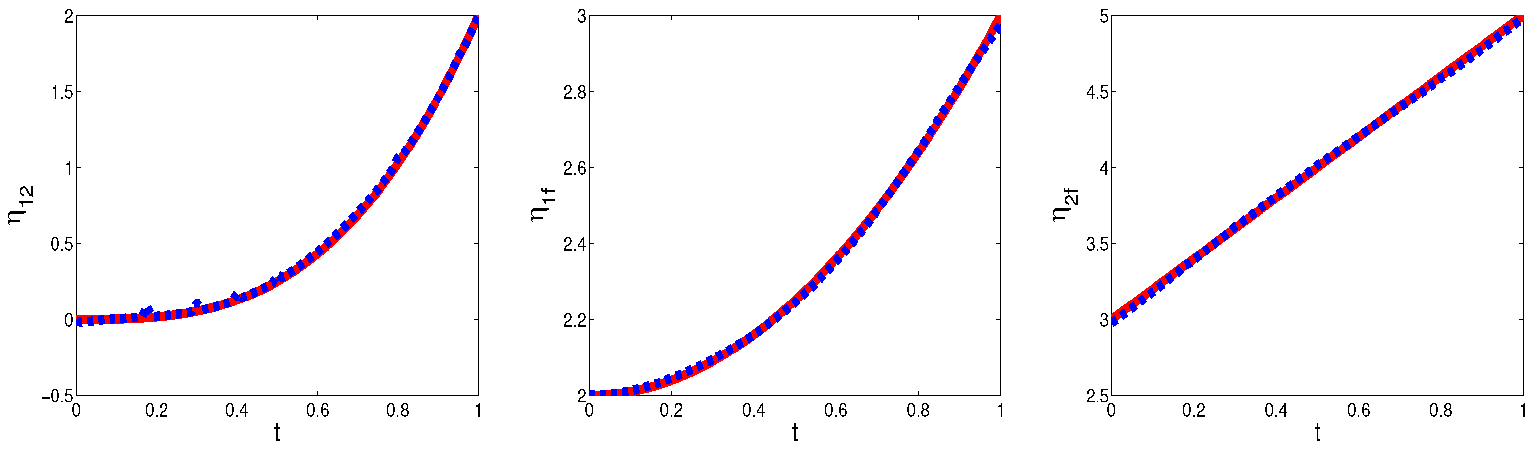
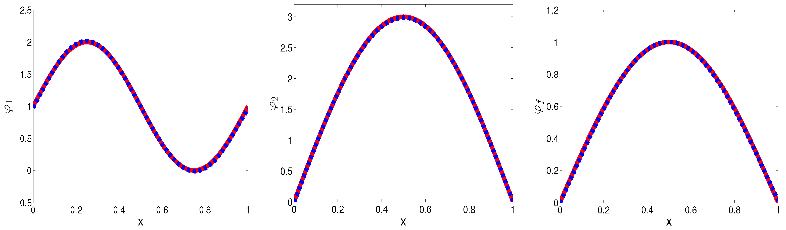
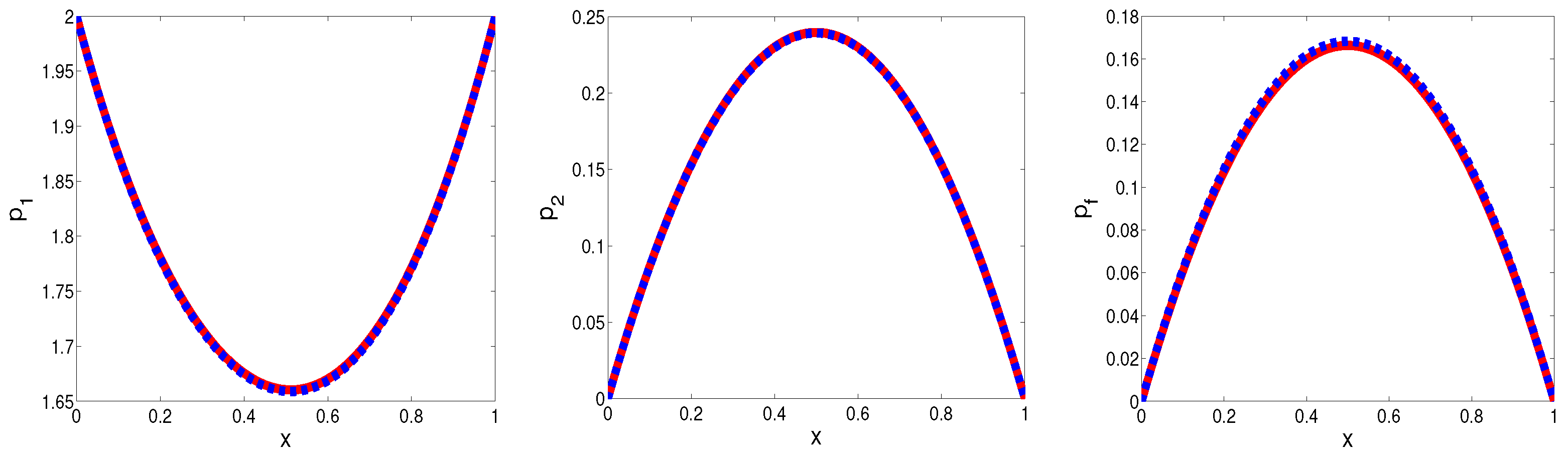
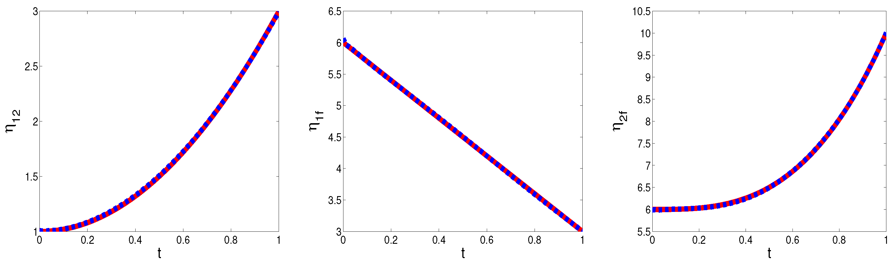
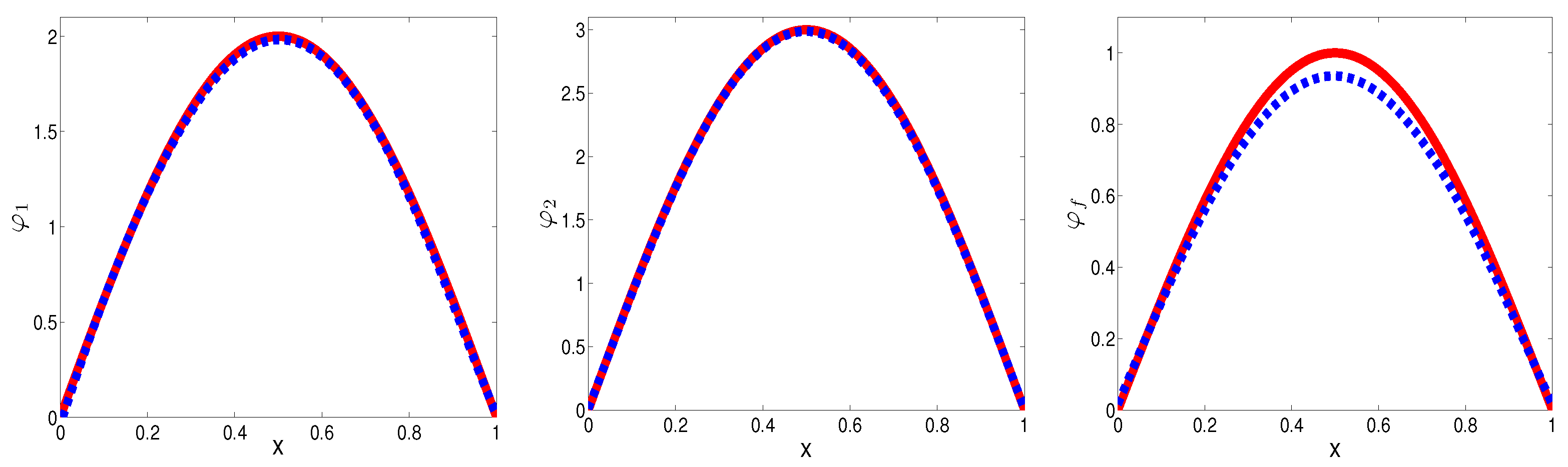
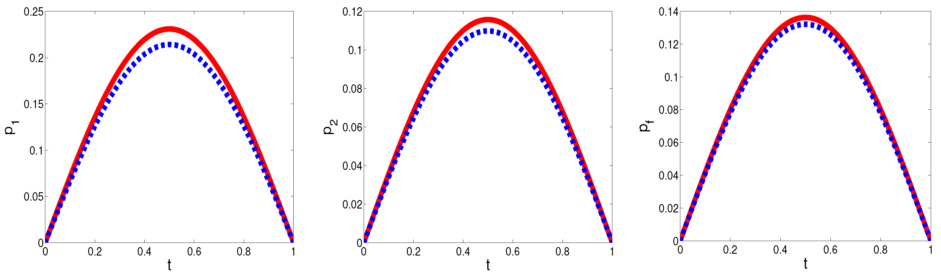
On Figure 1, Figure 2 and Figure 3, we plot the recovered and exact functions $\eta$, $\phi$ and the solution p at the last time level for ${\alpha }_1={\alpha }_2={\alpha }_f=0.5$. We observe a good fitting of the identified to the exact one.

In

Table 1. $RMSE$ errors of the identified solution $p_1$, $p_2$, $p_f$, Example 1.

$({\mathit{\alpha }}_1,{\mathit{\alpha }}_2,{\mathit{\alpha }}_3)$	${\mathit{\rho }}_0$	$\mathit{RMSE}\mathbf{\left(}{\mathit{p}}_{\mathbf{1}}\mathbf{\right)}$	$\mathit{RMSE}\mathbf{\left(}{\mathit{p}}_{\mathbf{2}}\mathbf{\right)}$	$\mathit{RMSE}\mathbf{\left(}{\mathit{p}}_{\mathit{f}}\mathbf{\right)}$
$(0.5,0.5,0.5)$	0.05	6.72434 × 10−4	1.45711 × 10−3	6.92054 × 10−5
$(0.5,0.5,0.5)$	0.01	7.88331 × 10−4	2.81139 × 10−4	8.49064 × 10−4
$(0.5,0.5,0.5)$	0.10	1.18239 × 10−3	5.98905 × 10−3	8.73955 × 10−4
$(0.3,0.6,0.8)$	0.05	1.32682 × 10−3	2.14994 × 10−3	1.70400 × 10−4
$(0.3,0.6,0.8)$	0.01	1.60764 × 10−3	2.89852 × 10−3	4.83800 × 10−4
$(0.3,0.6,0.8)$	0.10	3.69160 × 10−3	1.38909 × 10−3	9.28963 × 10−4

, we give the $RMSE$ error for different values of the deviation ${\rho }_0$ and fractional order. As can be expected, more precise results are obtained for ${\alpha }_1={\alpha }_2={\alpha }_3=0.5$ and a smaller deviation, but the influence of the value of ${\rho }_0$ is not so significant.

Example 2

(Perturbed data). Now, we consider another set of model parameters and functions:

$$\begin{array}{cc}& {\displaystyle k_1=2,k_2=2.5,k_f=0.5,{\eta }_{12}=1+2t^2,{\eta }_{1f}=6-3t,{\eta }_{2f}=6+4t^3,}\\ & {\displaystyle g_1=\left(\mathsf{\Gamma }(1+{\alpha }_1)+\frac{\mathsf{\Gamma }(1+2{\alpha }_1)}{\mathsf{\Gamma }(1+{\alpha }_1)}{t}^{{\alpha }_1}+\frac{\mathsf{\Gamma }(1+3{\alpha }_1)}{\mathsf{\Gamma }(1+2{\alpha }_1)}{t}^{2{\alpha }_1}\right)sin\left(\pi x\right),g_2=tsin\left(\pi x\right),g_3=0,}\\ & {\displaystyle {\phi }_1=2sin\left(\pi x\right),{\phi }_2=3sin\left(\pi x\right),{\phi }_f=sin\left(\pi x\right).}\end{array}$$

Numerical tests are performed for 36 points of measurements $M=L=6$, the same as in Example 1, where $N_x=N_t=80$, $T=1$, $\epsilon ={10}^{-3}$, ${\rho }_0=0.15$ in (25), ${\rho }_a=({\rho }_{a,1},{\rho }_{a,2},{\rho }_{a,f})$, and the following measurements:

$$\begin{array}{c}\hfill G_{l,m}^i=y_{i,l}^m+2{\rho }_{a,i}(\varrho (t^m,x_l)-0.5),i=1,2,f.\end{array}$$

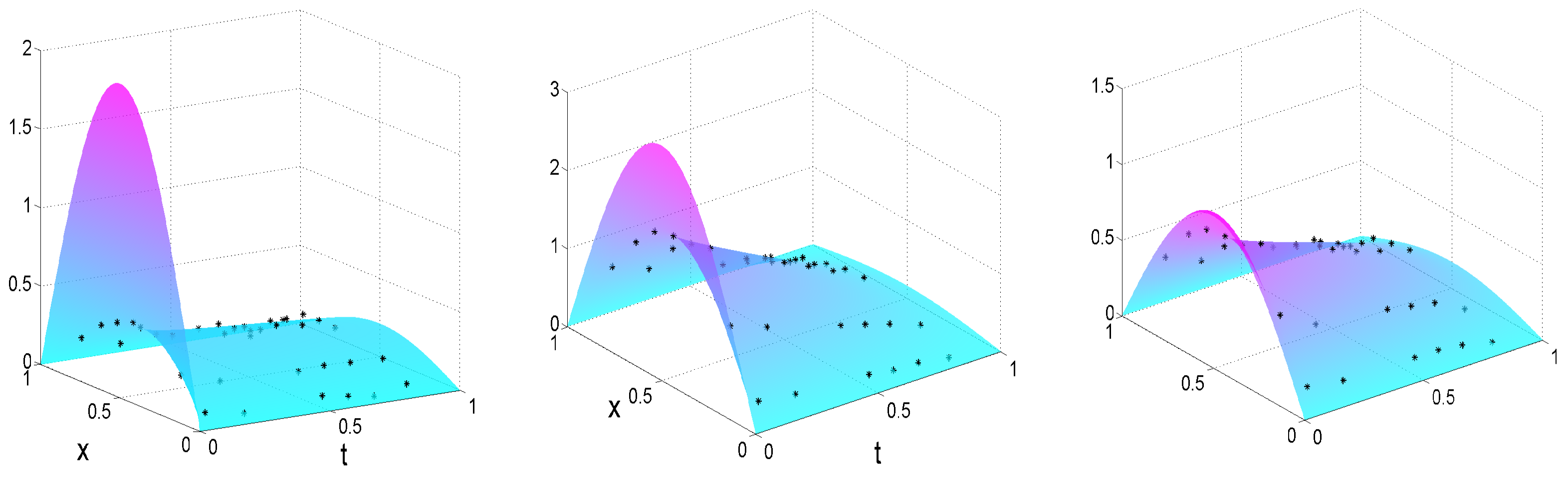
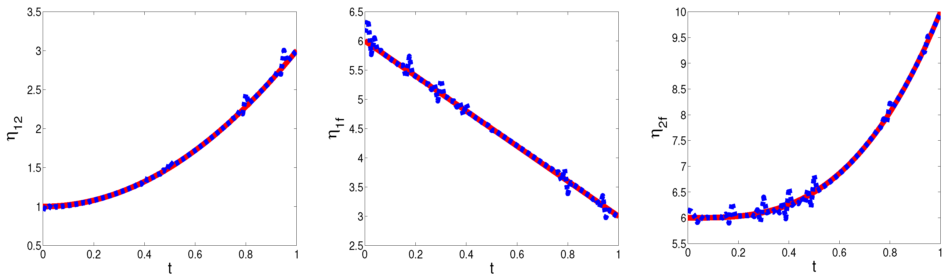
In Figure 4, we plot the exact solution and generated measurements for ${\rho }_{a,1}=0.035$, ${\rho }_{a,2}=0.03$, ${\rho }_{a,f}=0.04$, ${\alpha }_1={\alpha }_2={\alpha }_f=0.5$.

In

Table 2. Errors of the identified functions ${\eta }_{12}$, ${\eta }_{1f}$, ${\eta }_{2f}$, Example 2.

$({\mathit{\alpha }}_1,{\mathit{\alpha }}_2,{\mathit{\alpha }}_3)$	${\mathcal{E}}_{\mathit{a}}\left({\mathit{\eta }}_{12}\right)$	${\mathcal{E}}_{\mathit{a}}\left({\mathit{\eta }}_{1\mathit{f}}\right)$	${\mathcal{E}}_{\mathit{a}}\left({\mathit{\eta }}_{2\mathit{f}}\right)$	${\mathcal{E}}_{\mathit{r}}\left({\mathit{\eta }}_{12}\right)$	${\mathcal{E}}_{\mathit{r}}\left({\mathit{\eta }}_{1\mathit{f}}\right)$	${\mathcal{E}}_{\mathit{r}}\left({\mathit{\eta }}_{2\mathit{f}}\right)$
$(0.5,0.5,0.5)$	7.954 × 10−3	6.261 × 10−2	1.460 × 10−2	2.651 × 10−3	1.044 × 10−2	1.460 × 10−3
$(0.9,0.6,0.4)$	1.970 × 10−1	4.011 × 10−1	3.217 × 10−1	6.566 × 10−2	6.685 × 10−2	3.217 × 10−2

,

Table 3. Errors of the identified coefficients $k_1$, $k_2$, $k_f$, Example 2.

$({\mathit{\alpha }}_1,{\mathit{\alpha }}_2,{\mathit{\alpha }}_3)$	${\mathcal{E}}_{\mathit{a}}\left({\mathit{k}}_1\right)$	${\mathcal{E}}_{\mathit{a}}\left({\mathit{k}}_2\right)$	${\mathcal{E}}_{\mathit{a}}\left({\mathit{k}}_{\mathit{f}}\right)$	${\mathcal{E}}_{\mathit{r}}\left({\mathit{k}}_1\right)$	${\mathcal{E}}_{\mathit{r}}\left({\mathit{k}}_2\right)$	${\mathcal{E}}_{\mathit{r}}\left({\mathit{k}}_{\mathit{f}}\right)$
$(0.5,0.5,0.5)$	4.251 × 10−2	3.325 × 10−2	9.864 × 10−3	2.125 × 10−2	1.330 × 10−2	1.973 × 10−2
$(0.9,0.6,0.4)$	1.947 × 10−1	8.218 × 10−2	1.597 × 10−1	9.738 × 10−2	3.287 × 10−2	3.194 × 10−1

,

Table 4. Errors of the identified functions ${\phi }_1$, ${\phi }_2$, ${\phi }_f$, Example 2.

$({\mathit{\alpha }}_1,{\mathit{\alpha }}_2,{\mathit{\alpha }}_3)$	${\mathcal{E}}_{\mathit{a}}\left({\mathit{\phi }}_1\right)$	${\mathcal{E}}_{\mathit{a}}\left({\mathit{\phi }}_2\right)$	${\mathcal{E}}_{\mathit{a}}\left({\mathit{\phi }}_{\mathit{f}}\right)$	${\mathcal{E}}_{\mathit{r}}\left({\mathit{\phi }}_1\right)$	${\mathcal{E}}_{\mathit{r}}\left({\mathit{\phi }}_2\right)$	${\mathcal{E}}_{\mathit{r}}\left({\mathit{\phi }}_{\mathit{f}}\right)$
$(0.5,0.5,0.5)$	1.536 × 10−2	1.593 × 10−2	4.388 × 10−2	7.678 × 10−3	5.311 × 10−3	4.388 × 10−3
$(0.9,0.6,0.4)$	4.158 × 10−2	1.584 × 10−2	6.512 × 10−2	2.079 × 10−2	5.280 × 10−3	6.512 × 10−2

,

Table 5. Errors of the identified solution $p_1$, $p_2$, $p_f$, Example 2.

$({\mathit{\alpha }}_1,{\mathit{\alpha }}_2,{\mathit{\alpha }}_3)$	${\mathcal{E}}_{\mathit{a}}\left({\mathit{p}}_1\right)$	${\mathcal{E}}_{\mathit{a}}\left({\mathit{p}}_2\right)$	${\mathcal{E}}_{\mathit{a}}\left({\mathit{p}}_{\mathit{f}}\right)$	${\mathcal{E}}_{\mathit{r}}\left({\mathit{p}}_1\right)$	${\mathcal{E}}_{\mathit{r}}\left({\mathit{p}}_2\right)$	${\mathcal{E}}_{\mathit{r}}\left({\mathit{p}}_{\mathit{f}}\right)$
$(0.5,0.5,0.5)$	6.855 × 10−2	5.099 × 10−2	2.517 × 10−1	3.428 × 10−2	1.699 × 10−2	2.516 × 10−1
$(0.9,0.6,0.4)$	7.128 × 10−2	8.940 × 10−2	3.470 × 10−1	3.564 × 10−2	2.980 × 10−2	3.470 × 10−1

and

Table 6. $RMSE$ errors of the identified solution $p_1$, $p_2$, $p_f$, Example 2.

$({\mathit{\alpha }}_1,{\mathit{\alpha }}_2,{\mathit{\alpha }}_3)$	$\mathit{RMSE}\left({\mathit{p}}_1\right)$	$\mathit{RMSE}\left({\mathit{p}}_2\right)$	$\mathit{RMSE}\left({\mathit{p}}_{\mathit{f}}\right)$
$(0.5,0.5,0.5)$	3.519 × 10−3	3.282 × 10−3	1.826 × 10−2
$(0.9,0.6,0.4)$	1.984 × 10−2	8.395 × 10−3	6.160 × 10−3

, we give errors of the numerical solution obtained by the inverse problem for different values of the fractional order. In Figure 5, Figure 6, Figure 7, Figure 8, Figure 9 and Figure 10, we depict the corresponding exact and restored functions. In general, the numerical approach is efficient for recovering the diffusion coefficients, reaction term, initial functions, and solution p. We observe that more precise results are obtained for the moderate and equal values of the fractional orders ${\alpha }_i$, $i=1,2,f$. We may conclude that, for noisy data, the nonequal orders of the fractional derivatives affect the accuracy of the solution.

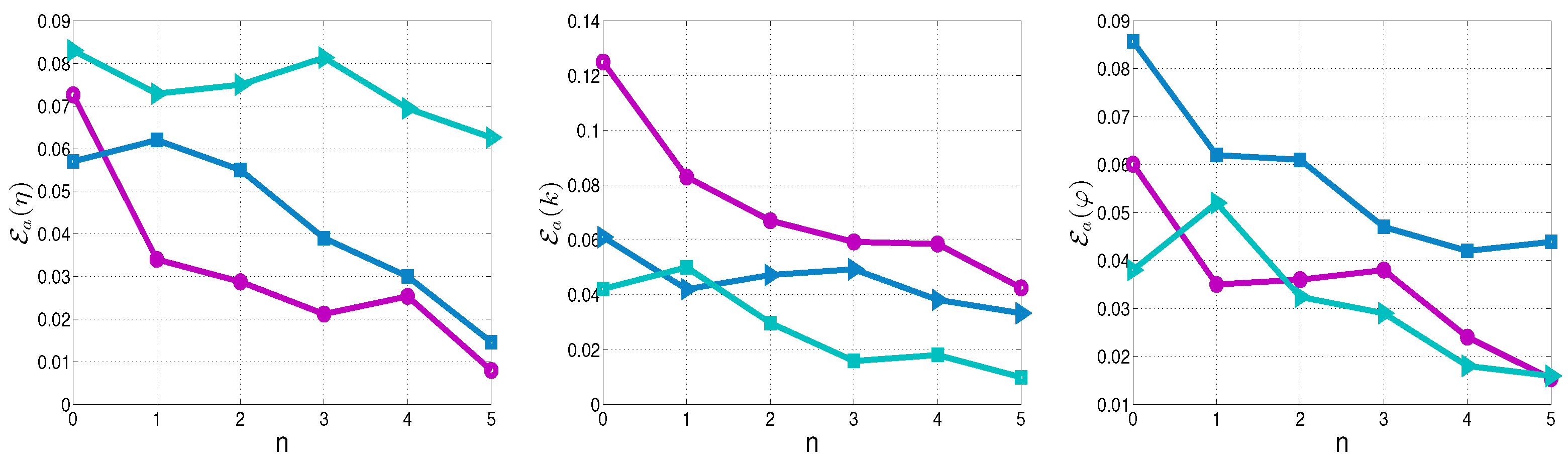
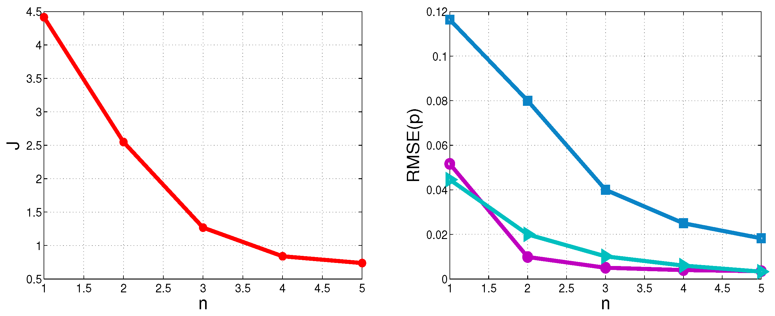
In Figure 11 and Figure 12, we illustrate the changes of the errors in the maximal norm of the restored parameters and the functional and $RMSE$ error at each iteration for ${\alpha }_1={\alpha }_2={\alpha }_f=0.5$.

For the considered set of measurements and deviations, the iterative process performs five iterations and stops since $J_6>J_5$.

10. Summary and Future Work

In this paper, an inverse problem for the estimation of the coefficients and initial condition of a model time-fractional parabolic system in porous media was studied. The inverse problem uses information about the pressures at a finite number of points in the space-time domain.

This paper is devoted to the theoretical analysis and numerical implementation of the 1D inverse problem, which is reduced to the minimization of a least-squares cost functional. The Frechet gradient of the functional was derived. Based on the explicit gradient formula, we described a CGM algorithm.

The numerical realization of the identification algorithm was proposed. The computational tests showed a good efficiency of the developed approach for simultaneously recovering the unknown diffusion coefficients, reaction terms, initial conditions, and the solution (pressure), even for noisy data. The different order of the fractional derivatives has a significant influence on the accuracy of the restored functions and solution. For ${\alpha }_i<0.25$ or ${\alpha }_i>0.9$, the algorithm fails to recover some of the parameters.

This present approach can be extended for multidimensional problems, but this will be undertaken in future work. Moreover, we plan to further improve the algorithm, applying the iterative regularization procedure of the CGM, such that it enhances the accuracy.

References

Alen, M.B. The Mathemaics of Fluid Flow through Porous Media, 1st ed.; Wiley: Hoboken, NJ, USA, 2021; p. 224. [Google Scholar]
Goltz, M.; Huang, J. Analytical Modeling of Solute Transport in Groundwater: Using Models to Understand the Effect of Natural Processes on Contaminant Fate and Transport; John Wiley & Sons, Inc.: Hoboken, NJ, USA, 2017; 155p. [Google Scholar]
Park, E.; Zhan, H. One-dimensional solute transport in a permeable reactive barrier–aquifer system. Water Resour. Res.2009, 45, W07502. [Google Scholar] [CrossRef]
Alaimo, G.; Piccolo, V.; Cutolo, A.; Deseri, L.; Fraldi, M.; Zingales, M. A fractional order theory of poroelasticity. Mech. Res. Commun.2019, 100, 103395. [Google Scholar] [CrossRef]
Goulart, A.G.; Lazo, M.J.; Suarez, J.M.S. A new parameterization for the concentration flux using the fractional calculus to model the dispersion of contaminants in the planetary boundary layer. Phys. A Stat. Mech. Its Appl.2019, 518, 38–49. [Google Scholar] [CrossRef]
Liu, F.J.; Li, Z.B.; Zhang, S.; Liu, H.Y. He’s fractional derivative for heat conduction in a fractal medium arising in silkworm cocoon hierarchy. Therm. Sci.2015, 19, 1155–1159. [Google Scholar] [CrossRef]
Mahiuddin, M.; Godhani, D.; Feng, L.; Liu, F.; Langrish, T.; Karim, M. Application of caputo fractional rheological model to determine the viscoelastic and mechanical properties of fruit and vegetables. Postharvest Biol. Technol.2020, 163, 111147. [Google Scholar] [CrossRef]
Tyrylgin, A.; Vasilyeva, M.; Alikhanov, A.; Sheen, D. A computational macroscale model for the time fractional poroelasticity problem in fractured and heterogeneous media. J. Comput. Appl. Math.2022, 418, 114670. [Google Scholar] [CrossRef]
Kandilarov, J.; Vulkov, L. Determination of concentration source in a fractional derivative model of atmospheric pollution. AIP Conf. Proc.2021, 2333, 090014. [Google Scholar]
Caputo, M. Vibrations of an infinite viscoelastic layer with a dissipative memory. J. Acoust. Soc. Am.1974, 56, 897–904. [Google Scholar] [CrossRef]
Jovanović, B.S.; Vulkov, L.G.; Delić, A. Boundary value problems for fractional PDE and their numerical approximation. In Numerical Analysis and Its Applications; Lecture Notes in Computer Science; Dimov, I., Faragó, I., Vulkov, L., Eds.; Springer: Berlin/Heidelberg, Germany, 2013; Volume 8236, pp. 38–49. [Google Scholar]
Kilbas, A.A.; Srivastava, H.M.; Trujillo, J.J. Theory and Applications of Fractional Differential Equations. In North-Holland Mathematics Studies, 1st ed.; North-Holland: Amsterdam, The Netherlands, 2006; Volume 204. [Google Scholar]
Podlubny, I. Fractional Differential Equations; Mathematics in Science and Engineering; Elsevier: Amsterdam, The Netherlands, 1998; Volume 198. [Google Scholar]
Gyulov, T.B.; Vulkov, L.G. A priory estimates for solutions of bounary value problems for a time fractional parabolic system of fractured porous media. AIP Conf. Proc.2023, 2953. accepted. [Google Scholar]
Koleva, M.N.; Vulkov, L.G. Numerical solution of a time fractional parabolic system in fractured porous media. AIP Conf. Proc.2023, 2953. accepted. [Google Scholar]
Gyulov, T.B.; Vulkov, L.G. Reconstruction of the lumped water-to-air mass transfer coefficient from final time or time-averaged concentration measurement in a model porous media. In Studies in Computational Intelligence; Springer: Berlin/Heidelberg, Germany, 2023; accepted. [Google Scholar]
Vabishchevich, P.N.; Denisenko, A.Y. Numerical methods for solving the coefficient inverse problem. Comput. Math. Model.1992, 3, 261–267. [Google Scholar] [CrossRef]
Liu, W.; Li, G.; Jia, X. Numerical simulation for a fractal MIM model for solute transport in porous media. J. Math. Res.2021, 13, 31–44. [Google Scholar] [CrossRef]
Raghavan, R. Fractional derivatives: Application to transient flow. J. Pet. Sci. Eng.2011, 80, 7–13. [Google Scholar] [CrossRef]
Zhou, H.W.; Yang, S.; Zhang, S.Q. Modeling non-Darcian flow and solute transport in porous media with the Caputo–Fabrizio derivative. Appl. Math. Model.2019, 68, 603–615. [Google Scholar] [CrossRef]
Asl, N.A.; Rostamy, D. Identifying an unknown time-dependent boundary source in time-fractional diffusion equation with a non-local boundary condition. J. Comput. Appl. Math.2019, 355, 36–50. [Google Scholar] [CrossRef]
Erfanian, M.; Hamed, Z.; Baghani, O. Solving an inverse problem for a time-fractional advection-diffusion equation with variable coefficients by rationalized Haar wavelet method. J. Comput. Sci.2022, 64, 101869. [Google Scholar] [CrossRef]
El Hamidi, A.; Kirane, M.; Tfayli, A. An Inverse Problem for a Non-Homogeneous Time-Space Fractional Equation. Mathematics2022, 10, 2586. [Google Scholar] [CrossRef]
Hasanov, A.H.; Romanov, V.G. Introduction to Inverse Problems for Differential Equations; Springer: Cham, Switzerland, 2017. [Google Scholar]
Li, G.; Jia, X.; Liu, W.; Li, Z. An inverse problem of determining fractional orders in a fractal solute transport model. arXiv2021, arXiv:2111.13013. [Google Scholar]
Wei, T.; Xian, J. Variational method for a backward problem for a time-fractional diffusion equation. ESAIM M2AN2019, 53, 1223–1244. [Google Scholar] [CrossRef]
Tikhonov, A.; Arsenin, V. Solutions of Ill-Posed Problems; Winston: Washington, DC, USA, 1977. [Google Scholar]
Alikhanov, A.A. A priori estimates for solutions of boundary value problems for fractional-order equations. Differ. Equ.2010, 46, 660–666. [Google Scholar] [CrossRef]
Chavent, G. Nonlinear Least Squares for Inverse Problems: Theoretical Foundations and Step-by-Step Guide for Applications; Scientific Computation; Springer: Dordrecht, The Netherlands, 2010. [Google Scholar]
Lesnic, D. Inverse Problems with Applications in Science and Engineering, 1st ed.; Chapman and Hall/CRC: New York, NY, USA, 2021. [Google Scholar]
Cai, M.; Li, C. Numerical Approaches to Fractional Integrals and Derivatives: A Review. Mathematics2020, 8, 43. [Google Scholar] [CrossRef]
Oldham, K.B.; Spanier, J. The Fractional Calculus; Academic Press: New York, NY, USA, 1974. [Google Scholar]
Zhang, Y.; Sun, Z.; Liao, H. Finite difference methods for the time fractional diffusion equationo non-uniform meshes. J. Comput. Phys.2014, 265, 195–210. [Google Scholar] [CrossRef]
Bakhvalov, N.S. Numerical Methods; Mir Publishers: Moscow, Russia, 1977; 663p, (Translated from Russian to English). [Google Scholar]
Samarskii, A.A.; Vabishchevich, P.N. Numerical Methods for Solving Inverse Problems in Mathematical Physics; de Gruyter: Berlin, Germany, 2007; 438p. [Google Scholar]
Figure 1.
Exact (solid line) and recovered (dashed line) functions , , , Example 1.
Figure 2.
Figure 3.
Exact (solid line) and recovered (dashed line) solutions , , at , Example 1.
Figure 4.
Exact solutions , , and generated measurements, Example 2.
Figure 5.
Exact (solid line) and recovered (dashed line) functions , , , , Example 2.
Figure 6.
Figure 7.
Exact (solid line) and recovered (dashed line) solutions , , at , , Example 2.
Figure 8.
Exact (solid line) and recovered (dashed line) functions , , , , , , Example 2.
Figure 9.
Figure 10.
Exact (solid line) and recovered (dashed line) solutions , , at , , , , Example 2.
Figure 11.
Errors in maximal norm at each iteration of the restored parameters , for (line with circles), (line with triangles), (line with squares), , Example 2.
Figure 12.
Changes of the functional and error at each iteration for (line with circles), (line with triangles), (line with squares), , Example 2.