
A Cotangent Fractional Derivative with the Application


Abstract
1. Introduction
- 1.
- The kernel operator is the exponential of the cotangent function,
- 2.
- The , and achieve a semi-group property,
- 3.
- If order , we obtain the RL-FD, C-FD, and RL-FI.
2. Preliminaries of FC
- 1.
- The left RL-FI of x of order is:
- 2.
- The right RL-FI of x of order is:
- 3.
- The left RL-FD of x of order is:
- 4.
- The right RL-FD of x of order is:
- 5.
- The left C-FD of x of order is:
- 6.
- The right C-FD of x of order is:
3. The Riemann–Liouville Cotangent Fractional Derivatives
- 1.
- .
- 2.
- .
- 3.
- .
- 4.
- .
- 2.
- Similar to 1.
- 3.
- Let , using the Lemma 1 and we have
- 4.
- Similar to 3.
- .
- Using Lemma 3 we obtain
- Lemma 3 is valid for any real σ.
4. The Laplace Transforms for Cotangent Fractional Integrals
5. The Caputo Cotangent Fractional Derivative
- 1.
- .
- 2.
- .
- Let then .
- implies that .
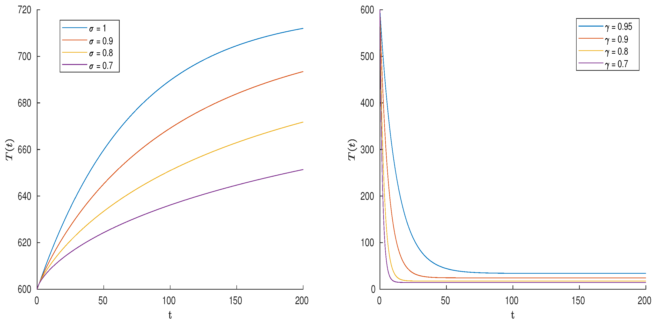
6. Application
7. Conclusions
Funding
Data Availability Statement
Acknowledgments
Conflicts of Interest
References
- Hilfer, R. (Ed.) Applications of Fractional Calculus in Physics; World Scientific: Singapore, 2000. [Google Scholar]
- Debnath, L. Recent applications of fractional calculus to science and engineering. Int. J. Math. Math. Sci. 2003, 2003, 3413–3442. [Google Scholar] [CrossRef]
- Kilbas, A.A.; Srivastava, H.M.; Trujillo, J.J. Theory and Applications of Fractional Differential Equations; Elsevier: Amsterdam, The Netherlands, 2006; Volume 204. [Google Scholar]
- Magin, R.L. Fractional Calculus in Bioengineering; Begell House Publishers: Danbury, CT, USA, 2006. [Google Scholar]
- Shah, K.; Jarad, F.; Abdeljawad, T. On a nonlinear fractional order model of dengue fever disease under Caputo-Fabrizio derivative. Alex. Eng. J. 2020, 59, 2305–2313. [Google Scholar] [CrossRef]
- Shah, K.; Alqudah, M.A.; Jarad, F.; Abdeljawad, T. Semi-analytical study of Pine Wilt Disease model with convex rate under Caputo-Febrizio fractional order derivative. Chaos Solitons Fractals 2020, 135, 109754. [Google Scholar] [CrossRef]
- Jarad, F.; Ugurlu, E.; Abdeljawad, T.; Baleanu, D. On a new class of fractional operators. Adv. Differ. Equ. 2017, 2017, 247. [Google Scholar] [CrossRef]
- Jarad, F.; Abdeljawad, T. Generalized fractional derivatives and Laplace transform. Discret. Contin. Dyn. S 2020, 13, 709–722. [Google Scholar] [CrossRef]
- Jarad, F.; Abdeljawad, T.; Alzabut, J. Generalized fractional derivatives generated by a class of local proportional derivatives. Eur. Phys. J. Spec. Top. 2017, 226, 3457–3471. [Google Scholar] [CrossRef]
- Jarad, F.; Alqudah, M.A.; Abdeljawad, T. On more general forms of proportional fractional operators. Open Math. 2020, 18, 167–176. [Google Scholar] [CrossRef]
- Rashid, S.; Jarad, F.; Noor, M.A.; Kalsoom, H.; Chu, Y.M. Inequalities by means of generalized proportional fractional integral operators with respect to another function. Mathematics 2019, 7, 1225. [Google Scholar] [CrossRef]
- Rahman, G.; Abdeljawad, T.; Jarad, F.; Nisar, K.S. Bounds of generalized proportional fractional integrals in general form via convex functions and their applications. Mathematics 2020, 8, 113. [Google Scholar] [CrossRef]
- Rahman, G.; Abdeljawad, T.; Jarad, F.; Khan, A.; Nisar, K.S. Certain inequalities via generalized proportional Hadamard fractional integral operators. Adv. Differ. Equ. 2019, 2019, 454. [Google Scholar] [CrossRef]
- Gambo, Y.Y.; Jarad, F.; Baleanu, D.; Abdeljawad, T. On Caputo modification of the Hadamard fractional derivatives. Adv. Differ. Equations 2014, 2014, 10. [Google Scholar] [CrossRef]
- Jarad, F.; Abdeljawad, T.; Baleanu, D. Caputo-type modification of the Hadamard fractional derivatives. Adv. Differ. Equ. 2012, 2012, 142. [Google Scholar] [CrossRef]
- Adjabi, Y.; Jarad, F.; Baleanu, D.; Abdeljawad, T. On Cauchy problems with Caputo Hadamard fractional derivatives. J. Comput. Anal. Appl. 2016, 21, 661–681. [Google Scholar]
- Khalil, R.; Al Horani, M.; Yousef, A.; Sababheh, M. A new definition of fractional derivative. J. Comput. Appl. Math. 2014, 264, 65–70. [Google Scholar] [CrossRef]
- Abdeljawad, T. On conformable fractional calculus. J. Comput. Appl. Math. 2015, 279, 57–66. [Google Scholar] [CrossRef]
- Katugampola, U.N. New approach to a generalized fractional integral. Appl. Math. Comput. 2011, 218, 860–865. [Google Scholar] [CrossRef]
- Katugampola, U.N. A new approach to generalized fractional derivatives. arXiv 2011, arXiv:1106.0965. [Google Scholar]
- Anderson, D.R.; Ulness, D.J. Newly defined conformable derivatives. Adv. Dyn. Syst. Appl. 2015, 10, 109–137. [Google Scholar]
- Anderson, D.R. Second–order self-adjoint differential equations using a proportional–derivative controller. Comm. Appl. Nonlinear Anal. 2017, 24, 17–48. [Google Scholar]
- Caputo, M.; Fabrizio, M. A new definition of fractional derivative without singular kernel. Progr. Fract. Differ. Appl. 2015, 1, 73–85. [Google Scholar]
- Losada, J.; Nieto, J.J. Properties of a new fractional derivative without singular kernel. Progr. Fract. Differ. Appl. 2015, 1, 87–92. [Google Scholar]
- Abdeljawad, T.; Baleanu, D. Monotonicity results for fractional difference operators with discrete exponential kernels. Adv. Differ. Equ. 2017, 2017, 78. [Google Scholar] [CrossRef]
- Abdeljawad, T.; Baleanu, D. On fractional derivatives with exponential kernel and their discrete versions. Rep. Math. Phys. 2017, 80, 11–27. [Google Scholar] [CrossRef]
- Atangana, A.; Baleanu, D. New fractional derivative with non-local and non–singular kernel. Thermal Sci. 2016, 20, 757. [Google Scholar] [CrossRef]
- Kochubei, A.N. General fractional calculus, evolution equations, and renewal processes. Integral Equ. Oper. Theory 2011, 71, 583–600. [Google Scholar] [CrossRef]
- Kilbas, A.A.; Saigo, M.; Saxena, R.K. Generalized Mittag-Leffler function and generalized fractional calculus operator. Integral Transform. Spec. Funct. 2004, 15, 31–49. [Google Scholar] [CrossRef]
- Jarad, F.; Abdeljawad, T.; Baleanu, D. On the generalized fractional derivatives and their Caputo modification. J. Nonlinear Sci. Appl. 2017, 10, 2607–2619. [Google Scholar] [CrossRef]
- Podlubny, I. Fractional Differential Equations; Academic Press: San Diego, CA, USA, 1999. [Google Scholar]
- Samko, S.G.; Kilbas, A.A.; Marichev, O.I. Fractional Integrals and Derivatives: Theory and Applications; Gordon and Breach: Yverdon, Switzerland, 1993. [Google Scholar]
- Habibi, F.; Birgani, O.; Koppelaar, H.; Radenović, S. Using fuzzy logic to improve the project time and cost estimation based on Project Evaluation and Review Technique (PERT). J. Proj. Manag. 2018, 3, 183–196. [Google Scholar] [CrossRef]
- Chandok, S.; Sharma, R.K.; Radenović, S. Multivalued problems via orthogonal contraction mappings with application to fractional differential equation. J. Fixed Point Theory Appl. 2021, 23, 14. [Google Scholar] [CrossRef]
- Stojiljković, V.; Ramaswamy, R.; Ashour Abdelnaby, O.A.; Radenović, S. Riemann-Liouville Fractional Inclusions for Convex Functions Using Interval Valued Setting. Mathematics 2022, 10, 3491. [Google Scholar] [CrossRef]
- Sadek, L. Controllability and observability for fractal linear dynamical systems. J. Vib. Control 2022, 10775463221123354. [Google Scholar] [CrossRef]
- Sadek, L.; Bataineh, A.S.; Talibi Alaoui, H.; Hashim, I. The Novel Mittag-Leffler–Galerkin Method: Application to a Riccati Differential Equation of Fractional Order. Fractal Fract. 2023, 7, 302. [Google Scholar] [CrossRef]
- Sadek, L. Stability of conformable linear infinite-dimensional systems. Int. J. Dyn. Control 2022, 11, 1276–1284. [Google Scholar] [CrossRef]
- Alipour, M.; Soradi Zeid, S. Optimal control of Volterra integro-differential equations based on interpolation polynomials and collocation method. Comput. Methods Differ. Equ. 2023, 11, 52–64. [Google Scholar]
- Zhao, W.; Gunzburger, M. Stochastic Collocation Method for Stochastic Optimal Boundary Control of the Navier–Stokes Equations. Appl. Math. Optim. 2023, 87, 6. [Google Scholar] [CrossRef]
- Oqielat, M.A.N.; Eriqat, T.; Al-Zhour, Z.; Ogilat, O.; El-Ajou, A.; Hashim, I. Construction of fractional series solutions to nonlinear fractional reaction–diffusion for bacteria growth model via Laplace residual power series method. Int. J. Dyn. Control 2023, 11, 520–527. [Google Scholar] [CrossRef]
- Kermack, W.O.; McKendrick, A.G. A contribution to the mathematical theory of epidemics. Proc. R. Soc. Lond. Ser. A Contain. Pap. Math. Phys. Character 1927, 115, 700–721. [Google Scholar]
- Sene, N. SIR epidemic model with Mittag-Leffler fractional derivative. Chaos Solitons Fractals 2020, 137, 109833. [Google Scholar] [CrossRef]
- Khan, M.A.; Ismail, M.; Ullah, S.; Farhan, M. Fractional order SIR model with generalized incidence rate. AIMS Math. 2020, 5, 1856–1880. [Google Scholar] [CrossRef]
- Naik, P.A. Global dynamics of a fractional-order SIR epidemic model with memory. Int. J. Biomath. 2020, 13, 2050071. [Google Scholar] [CrossRef]
- Taghvaei, A.; Georgiou, T.T.; Norton, L.; Tannenbaum, A. Fractional SIR epidemiological models. Sci. Rep. 2020, 10, 20882. [Google Scholar] [CrossRef] [PubMed]
- Dasbasi, B. Stability analysis of an incommensurate fractional-order SIR model. Math. Model. Numer. Simul. Appl. 2021, 1, 44–55. [Google Scholar]
- Kilicman, A. A fractional order SIR epidemic model for dengue transmission. Chaos Solitons Fractals 2018, 114, 55–62. [Google Scholar]
- Karaji, P.T.; Nyamoradi, N. Analysis of a fractional SIR model with general incidence function. Appl. Math. Lett. 2020, 108, 106499. [Google Scholar] [CrossRef]
- Jena, R.M.; Chakraverty, S.; Baleanu, D. SIR epidemic model of childhood diseases through fractional operators with Mittag-Leffler and exponential kernels. Math. Comput. Simul. 2021, 182, 514–534. [Google Scholar] [CrossRef]

Disclaimer/Publisher’s Note: The statements, opinions and data contained in all publications are solely those of the individual author(s) and contributor(s) and not of MDPI and/or the editor(s). MDPI and/or the editor(s) disclaim responsibility for any injury to people or property resulting from any ideas, methods, instructions or products referred to in the content. |
© 2023 by the author. Licensee MDPI, Basel, Switzerland. This article is an open access article distributed under the terms and conditions of the Creative Commons Attribution (CC BY) license (https://creativecommons.org/licenses/by/4.0/).
Share and Cite
Sadek, L. A Cotangent Fractional Derivative with the Application. Fractal Fract. 2023, 7, 444. https://doi.org/10.3390/fractalfract7060444
Sadek L. A Cotangent Fractional Derivative with the Application. Fractal and Fractional. 2023; 7(6):444. https://doi.org/10.3390/fractalfract7060444
Chicago/Turabian StyleSadek, Lakhlifa. 2023. "A Cotangent Fractional Derivative with the Application" Fractal and Fractional 7, no. 6: 444. https://doi.org/10.3390/fractalfract7060444
APA StyleSadek, L. (2023). A Cotangent Fractional Derivative with the Application. Fractal and Fractional, 7(6), 444. https://doi.org/10.3390/fractalfract7060444