1. Introduction
The study of effective numerical calculation methods for FBSDEs has become a hot topic in recent years due to their continuous development in both theory and practical applications. Because the solutions of FBSDEs are rarely found in real problems, numerical methods are a good choice. In 1990, Pardoux and Peng [
1] proved the existence and uniqueness of the nonlinear BSDE solution under standard conditions. After that, the study of FBSDEs became more and more popular. In contrast, the research results of coupled FBSDEs are lower than those of decoupled FBSDEs.
Currently, because of the computational complexity in the field of numerical experiments, coupled FBSDEs develop more slowly than decoupled FBSDEs. Because the analytic solutions of FBSDEs are rarely found in real problems, numerical solutions have become a good choice. Many researchers have tried to solve this problem. Generally, it can be divided into the following three main types of strategies.
The first strategy is to use fixed point theory (one can refer to the literature [
2,
3]). The second strategy utilizes the parabolic PDE to solve the FBSDE based on the general stochastic parabolic PDE discretization (for details, see [
4,
5,
6]). The third strategy is based on Fourier transform (such as [
7,
8,
9,
10]). Among these numerical methods, some are higher-order numerical methods that have high convergence rates, such as [
11,
12,
13,
14,
15].
However, coupled FBSDEs are a concept that has a wider range (e.g., coupled FBSDEs were used to simulate large investors who influence the stock price of financial markets). There are also some methods to solve this problem. Bender and Zhang [
16], who proved the convergence of time discretization and Markov iteration, laid the foundation for the numerical algorithm simulation of multidimensional coupled FBSDEs. In addition, based on FBSDE theory, Zhao, Fu, and Zhou [
17] investigated a new type of high-order multi-step scheme for coupled FBSDEs. Recently, Huijskens, Ruijter, and Oosterlee [
18] expanded the Fourier cos method to coupled FBSDEs with three numerical methods (i.e., explicit method, local method and global method), which had expected convergence and efficiency. Nam and Xu [
19] proved the solution of coupled FBSDEs is existential by using purely probabilistic methods to obtain semilinear parabolic PDEs. Inspired by these papers, we expand the idea that multidimensional coupled FBSDEs can be solved using the fractional Fourier transform to obtain the numerical solution of Equation (1). In addition, in recent years, deep learning methods have also been introduced in the numerical field [
20,
21,
22]. These algorithms are highly accurate, but at the same time, they are expensive to run. Therefore, this paper differs from other papers in the following aspects:
- (1)
Proving the theorem in different ways to ensure that the algorithm of fractional fast Fourier transform can be retained during numerical experiments.
- (2)
The numerical experiments were verified with coupled FBSDEs in different situations.
The organization of this paper is as follows:
Section 2 will provide some assumptions about coupled FBSDEs. We use the classical Euler scheme for the forward process of FBSDE, which was applied to decoupled FBSDEs by Zhao et al. [
23], to obtain the flexibility of the proposed calculation methods. For the backward process, the theta scheme will be used. In
Section 3, by incorporating the Fourier variations, we expand a discretization of general coupled FBSDEs. In
Section 4, three different approaches for dealing with the part of the coupling are described. In
Section 5, six numerical experiments are discussed to verify the numerical methods. Finally, we summarize some conclusions in
Section 6.
2. Assumptions and Discretization of the Coupled FBSDEs
Now, from this section, we studied the numerical calculation method of coupled FBSDEs (1) investigated by the following:
where
is an
-dimensional forward stochastic differential equation (FSDE), and
is a one-dimensional backward stochastic differential equation(BSDE).
and
are the initial condition of the FSDE and the end condition of the BSDE, respectively.
is a control process.
are the drift terms of the FSDE,
are diffusion terms of the FSDE, and
is defined on the probability space
with
the natural
-algebra generated by
, which is a standard
-dimensional normal Brownian motion process and satisfies the usual conditions. Here,
is called the generator function. The symbol
denotes the transpose of a vector.
We first introduce some definitions and assumptions that underpin the proposed algorithm. Then, we elaborate the discretization of the normal coupled FBSDEs, which is the foundation for the following content.
2.1. Definitions and Assumptions
Following the survey papers [
18,
24,
25], we provide the following standard definitions and assumptions. We define
as the set of
-adapted processes
that are square integrable, i.e.,
where
is the standard Euclidean norm in the Euclidean space. Denote
as the set of absolutely integrable processes. A triple set of processes (
X,
Y,
Z) is an adapted solution of Equation (1) if it satisfies (1) almost surely and belongs to
. In order to ensure the existence of the solution to Equation (1) and the validity of the numerical algorithm, we provide some assumptions [
5] as follows:
- (1)
The functions
and
are uniformly Lipschitz in
, for
. For example,
should satisfy
where
and
is the Lipschitz constant.
- (2)
The functions
,
and
satisfy the linear growth conditions as follows:
where
are constants.
- (3)
The diffusion has bounded second derivatives with positive lower and upper bounds.
- (4)
and , where is a function of and is the weak derivative symbol for .
Assumptions (1)–(4) can ensure that the solution
to the coupled FBSDE (1) is existential and unique. If the function
or
does not satisfy assumption (4), we can truncate in bounds (for details, see [
7]).
In the next subsection, we will discretize the FSDE in Equation (1) by using the Euler scheme and the BSDE in Equation (1) by -scheme.
2.2. Discretization of the General Coupled FBSDEs
It is classical to approximate the real solution of the FSDE by using the scheme of the Euler discretization. Consider a partition
of time grid
with time steps
, for
. For illustrative convenience, we denote
and
. We rewrite the local evolution of the FSDE in the time interval [
to the following form:
The discretization of the FSDE is:
The Equation (3) can also be explained as a left point approximation of Equation (2).
is an
-adapted process, so for both sides of Equation (4), we should adopt conditional expectations and use the
-scheme method to approximate the integral:
where
and
denotes
. We first multiply both sides of Equation (4) by
. Then, also taking conditional expectations, similar to Equation (5), we get:
The terminal values
and
can be obtained by using
because of a result of the Nonlinear Feynman-Kac Theorem [
25,
26]. Then we have:
with
as a gradient operator. The above equations are the basis of the following numerical methods. Since
in Equation (3) is a Markov process, we use a discrete-time approximation
for
in the BSDE. Then we have:
where
and
. In Equation (8), when setting
, we will get an explicit scheme for
. Based on observations of Equations (8) and (9), the numerical iteration of the BSDE lies in conditional expectations. In the next section, we will introduce the fractional fast Fourier transform (FrFFT) method to transfer the iteration to the Fourier space so that Equations (8) and (9) iterate smoothly.
3. Fractional Fast Fourier Transform Method
In this section, we derive a Fourier transform for Equations (7)–(9) to transfer the iteration to the Fourier space. Because the three existing algorithms differ from this scheme in the next section, the final FrFFT method used in the three algorithms is different in this section.
The conditional expectations are formed like the two equations below:
Since the evolution of
from Equation (3) is known, let
and
). Then, we have:
where
is the
row vector of
.
For convenience and clarity, we consider the following substitutions:
We rewrite Equations (7)–(9):
We consider the Fourier transform of a function
as:
and the Fourier inverse transform in the same way:
where
and
. We then need to numerically calculate the above two equations, truncating the integral with a sufficiently large region
and
with:
We get the approximation of integrals by the midpoint rule:
where
, and
We compute
by Equation (14) on
-grid and
by Equation (15) on
-grid. For efficiency, Equations (14) and (15) are computed by the FrFFT, which can be reviewed in [
7,
27]. We first introduce a one-dimensional situation and then generalize to a multidimensional one with the help of the one-dimensional situation.
Let
then
and
where
, and
. The appendix in [
7] has been demonstrated by the ι-multidimensional case of Equation (14). We will generalize Equation (15) to a
-multidimensional situation. Consider the
-dimensional integral,
where
To review this
-dimensional sum, we can carry out the caculation as follows.
where
Each problem is able to be calculated by the one-dimensional FrFFT [
28].
The Fourier transform is performed on both sides of Equations (11)–(13). In addition, we can get that
is represented by
for some function
.
To approximate the two equations, we introduce Lemma 1 and Theorem 1.
Lemma 1 ([29]). If , thenwhereis the characteristic function ofandcan be denoted by Theorem 1. If , then Proof. For the first equation, since
then we have
Let
. Then we get
. Since
we have
□
We now have the approximation of
.
where
However, it still does not provide an implementable solution for the decoupling case. In the next section, we will provide the detailed numerical algorithms to implement the above theory.
4. Numerical Algorithms of Coupled FBSDE Combined with FrFFT
In this section, to verify the effectiveness of Theorem 1, we refer to three algorithms in [
18]. In order to iterate, three algorithms need to be transformed.
4.1. Explicit Algorithm
We apply the technique from [
30]. Suppose the time step
to be small enough. For the processes
, there is an approximation of the positive process:
Equation (23) differs from Equation (3), where the right-point approximation is applied.
Because of the approximation of the different forward process
, the characteristic functions of
are also different. However, the differences are minimal because we just need to replace
in Equation (18) with
:
Furthermore, we have to replace
with
in Equations (10)–(13) and Equations (19)–(22).
where
and
where
Based on the above analysis, we give the following detailed Algorithm 1 to implement the numerical solution to Equation (1):
| Algorithm 1. Explicit algorithm |
| Initialization: |
| 1: Calculate and applying Equation (14) by FrFFT on the -grid. |
| Main loop: |
| 2: for to 1 do |
| 3: Calculate and via Equations (31) and (32). |
| 4: Calculate and applying Equation (15) by FrFFT on the -grid. |
| 5: Do Picard iteration times for Equation (26) to get y(tm, x) on the -grid. |
| 6: Get on the -grid. |
| 7: if then |
| 8: Calculate and applying Equation (14) by FrFFT on the -grid. |
| 9: end if |
| 10: end for |
| 11: if is not on the -grid then |
| 12: The cubic spline is interpolated on the -grid to get the value at . |
| 13: end if |
The following calculations are done when calculating the approximate values of the time :
Calculation of the function on the -grid in operations.
Computation of , and on the -grid in operations.
Computation of and on the -grid in operations.
Computation of on the -grid in operations.
Computation of the cubic spline on the -grid in operations.
The overall complexity of the explicit algorithm is , where is the number of components for .
Different: Each iteration is made on the -grid. Finally, at , the cubic spline is used to get the value at point .
4.2. Local Algorithm
We consider the iteration of each time interval
for
. Then one obtains an iteration that is similar to the method of [
17].
Unlike in the literature [
18], since the algorithm in this paper is performed on the grid for each iteration, each iteration needs to use the cubic spline to get the value of the corresponding point
at
. This allows the next iteration to proceed smoothly.
We denote by
the number of local iterations per time interval and
the current local iteration. Furthermore, we denote by
, and
respectively, the value of
and
in iteration
. Finally, we denote the values by
and
at
on the
-grid using the cubic spline. The cubic spline is interpolated on the
-grid to get the value of
and
in local iteration. Then, Equation (18) will be rewritten by:
However, we do not have functions with
and
at the iteration
and time point
, so we apply the previous iteration for approximating Equation (33), i.e.,
Furthermore, their derivations do not change.
where
and
where
Based on the above analysis, we give the following detailed Algorithm 2 to implement the numerical solution to Equation (1):
| Algorithm 2. Local algorithm |
| Initialization: |
| 1: Calculate and applying Equation (14) by FrFFT on the -grid. |
| 2: Calculate and by terminal conditions. |
| Main loop: |
| 3: for to 1 do |
| 4: |
| 5: |
| 6: for to do |
| 7: Calculate and via Equations (41) and (42). |
| 8: Calculate and applying Equation (15) by FrFFT on the -grid. |
| 9: Do Picard iteration times for Equation (36) to get on the -grid. |
| 10: Get on the -grid. |
| 11: if is not on the -grid then |
| 12: The cubic spline is interpolated on the x-grid to get the value of and at . |
| 13: end if |
| 14: if then |
| 15: Break. |
| 16: end if |
| 17: if then |
| 18: Calculate and applying Equation (14) by FrFFT on the -grid. |
| 19: end if |
| 20: end for |
| 21: end for |
The total complexity of the local algorithm is .
Different: Each iteration uses the cubic spline to get the desired value (i.e.,).
4.3. Global Algorithm
Finally, we can use one of the techniques proposed in [
16] that uses an iterative process over the entire time domain. We denote by
the number of global iterations, with
as the current global iteration. Furthermore, we denote by
and
respectively the value of
and
in iteration
. Finally, denote by the values of
and
at
on the
-grid using the cubic spline in the
iteration. Then the Equation (18) will be rewritten by:
However, we do not have functions with
and
at iteration
and time point
, so we also apply the previous iteration:
Using same logic as in
Section 4.2, we have:
where
and
where
Then the process of Algorithm 3 is as follows:
| Algorithm 3. Global algorithm |
| Initialization: |
| 1: Calculate and applying Equation (14) by FrFFT on the -grid. |
| Main loop: |
| 2: for to 1 do |
| 3: |
| 4: |
| 5: end for |
| 6: for to do |
| 7: for to 1 do |
| 8: Calculate and via Equations (51) and (52). |
| 9: Calculate and applying Equation (15) by FrFFT on the -grid. |
| 10: Do Picard iteration times for Equation (36) to get on the -grid. |
| 11: Get on the -grid. |
| 12: if is not on the -grid then |
| 13: The cubic spline is interpolated on the x-grid to get the value of and at . |
| 14: end if |
| 15: if then |
| 16: Calculate and applying Equation (14) by FrFFT on the -grid. |
| 17: end if |
| 18: end for |
| 19: if then |
| 20: Break. |
| 21: end if |
| 21: end for |
The overall complexity of the global algorithm is .
Different: Like the local algorithm, each iteration uses the cubic spline to get the desired value (i.e., ).
5. Numerical Experiments
In this section, we analyze several examples using the numerical methods developed above (Algorithm 1, Algorithm 2 and Algorithm 3) and analyze their results. In principle, the method can be applied to any dimension. However, due to the curse of dimensionality, it can compute intuitively in low dimensions. So, in order to display the experimental results, we only consider one-dimensional components; that is, has one component. MATLAB 9.12.0.1884302 was used for the computations, with an Intel(R) Pentium(R) CPU 4415U @ 2.30GHz and 4.00 GB of RAM.
For the local algorithm and the global algorithm, we use stopping criteria to determine when iterations should be stopped. and are set to . Here we apply the same type of stopping criterion for Picard iterations. The errors in all experiments in this section are absolute errors, which are defined as for and for .
Due to the Fourier method used in this paper, the integration interval
is referenced by [
10,
31] and the integration interval
is referenced by [
7].
For each method, we tested the following
schemes:
5.1. Example 1: A Decoupled Example
We consider the following decoupled FBSDE:
where
The solution of Equation (53) is given by:
In this experiment, we use
and
and set
and
. It is known that the exact solution is
. Since
and
are constants, the result of this example can be obtained directly using ordinary numerical methods without three algorithms mentioned in
Section 4. First, we analyze the error in the approximations of
and
of different values of
. The error is listed in
Table 1, where the approximations are obtained by the scheme A. Furthermore, the error in the approximation of
and
can be found in
Figure 1.
In
Table 1 and
Figure 1, we find that the error is accepted. What is more, with the increase of
and
, the error gradually becomes smaller. The method is stable and the calculation time is fast.
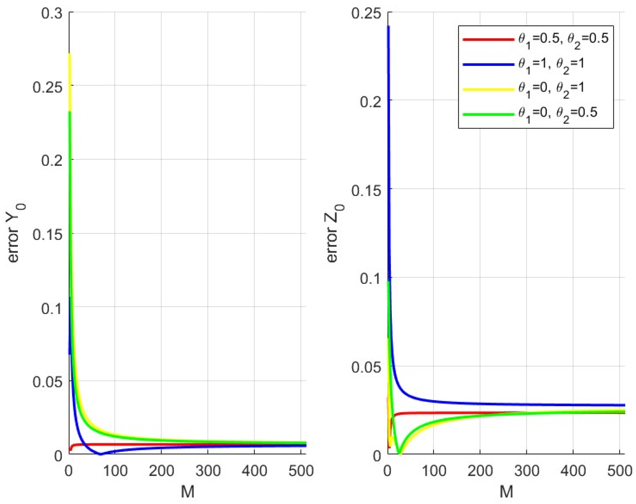
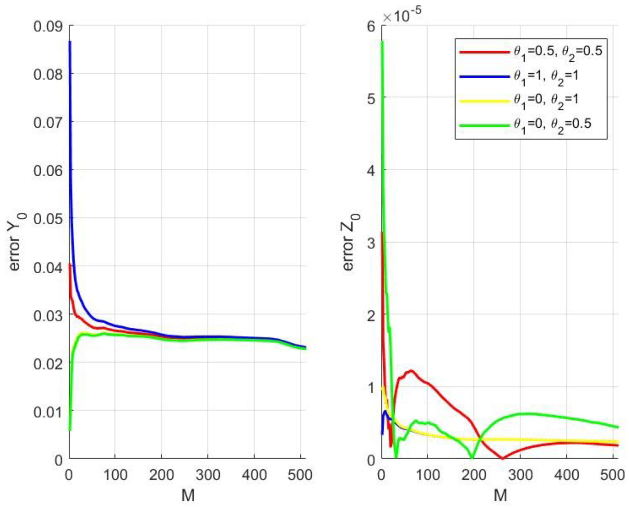
5.2. Example 2: Forward Process Depending on Xt
We consider the following coupled FBSDE:
where
The solution of Equation (54) is given by:
For the experiment, we use and and set and . It is known that the exact solution is .
Because in the case of this example, the effect of the local algorithm and the global algorithm is the same, we only show the result of one of them as follows:
Table 2 shows the error for the approximations of
and
for different values of
and
. In addition, we observe that the error in the approximation is mainly determined by the number of time points
; as the value of
increases, the error stops decreasing at a certain point. Therefore, we pay more attention to the error behavior when the number of time points changes. For all the next numerical tests, we will use
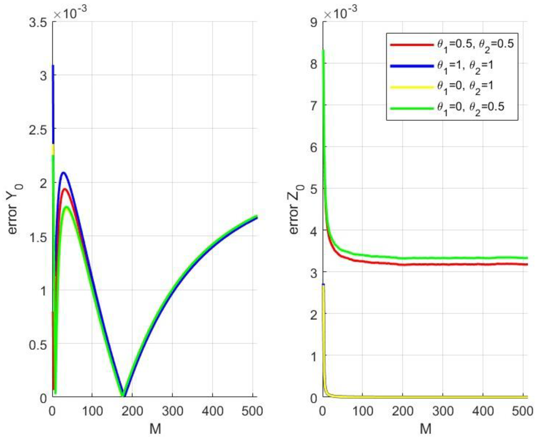
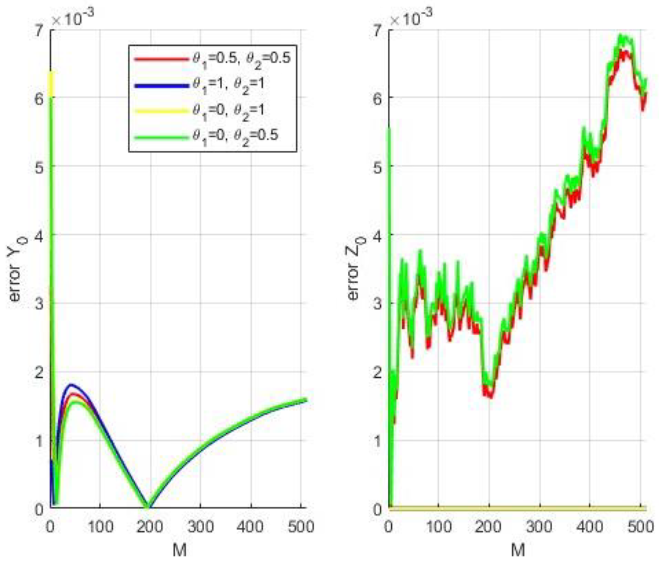
to ensure sufficient accuracy. In
Figure 2 and
Figure 3, the errors of
achieve convergence as
becomes larger in all schemes. The errors of
also achieve convergence in schemes B and C. However, the error of the explicit algorithm is significantly larger than that of the local algorithm. In short, although the processes of schemes A and D of the error of
are oscillating, they eventually converge at a very small number.
5.3. Example 3: Diffusion Depending on Yt
We consider the following coupled FBSDE [
5]:
where
and
The solution of Equation (55) is given by:
For the experiment, we use and and set and . The correct solution is .
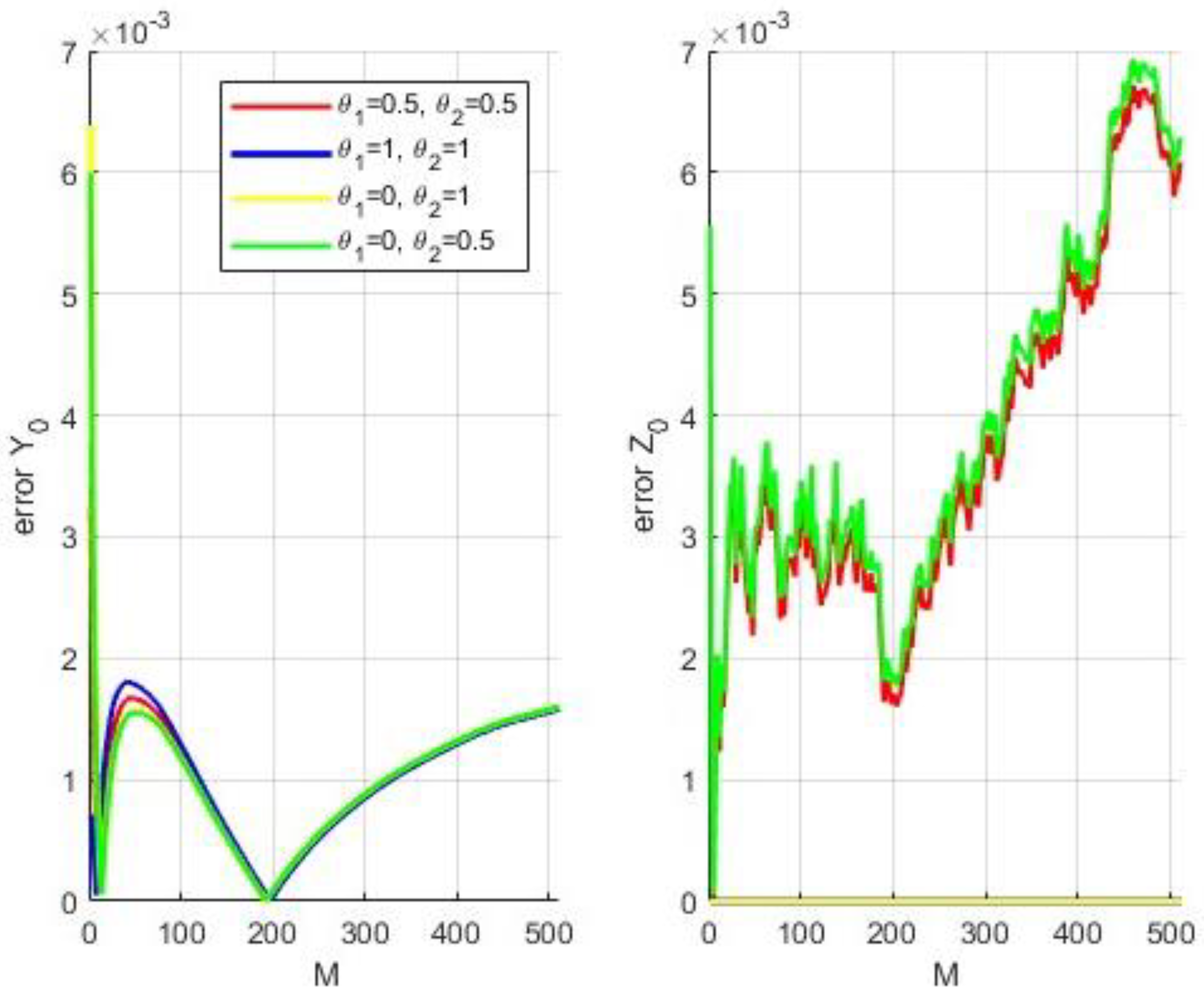
The results of the explicit algorithm, the local algorithm, and the global algorithm can be found separately in
Figure 4,
Figure 5 and
Figure 6. The error of
does not differ significantly in the three algorithms and actually converges as the value of
becomes larger. For the error of
in all schemes, we observe that the explicit method converges. For the local algorithm and global algorithm, scheme B and scheme C are smoother than other schemes. However, they are still convergent.
Table 3 shows the CPU times for the three algorithms. Since the time of each scheme (B, C, and D) in the same algorithm is approaching, these will not be shown here. Here, we note that the explicit algorithm is remarkably faster than others. The CPU speeds of the local algorithm and the global algorithm are close.
5.4. Example 4: Drift Depending on Zt
We consider the following coupled FBSDE [
17]:
where
The solution of Equation (56) is given by:
For the experiment, we use and and set and . It is known that the exact solution is .
The results for the three algorithms can be found in
Figure 7,
Figure 8 and
Figure 9. For
, we observe that the three algorithms obviously converge. For
, scheme B and scheme C in the three algorithms are smoother than other schemes. Scheme A and scheme D have local oscillations, but overall, their errors are still small.
Table 4 shows the CPU times for the explicit, local, and global algorithms. Here, only the case of scheme A is shown. We noticed that the explicit algorithm is remarkably faster than the others. The CPU speeds of the local algorithm and the global algorithm are similar.
5.5. Example 5: Drift Depending on Zt
We consider the following coupled FBSDE [
17]:
where
The solution of Equation (57) is given by:
In the experiment, we use and and set , and . It is known that the exact solution is .
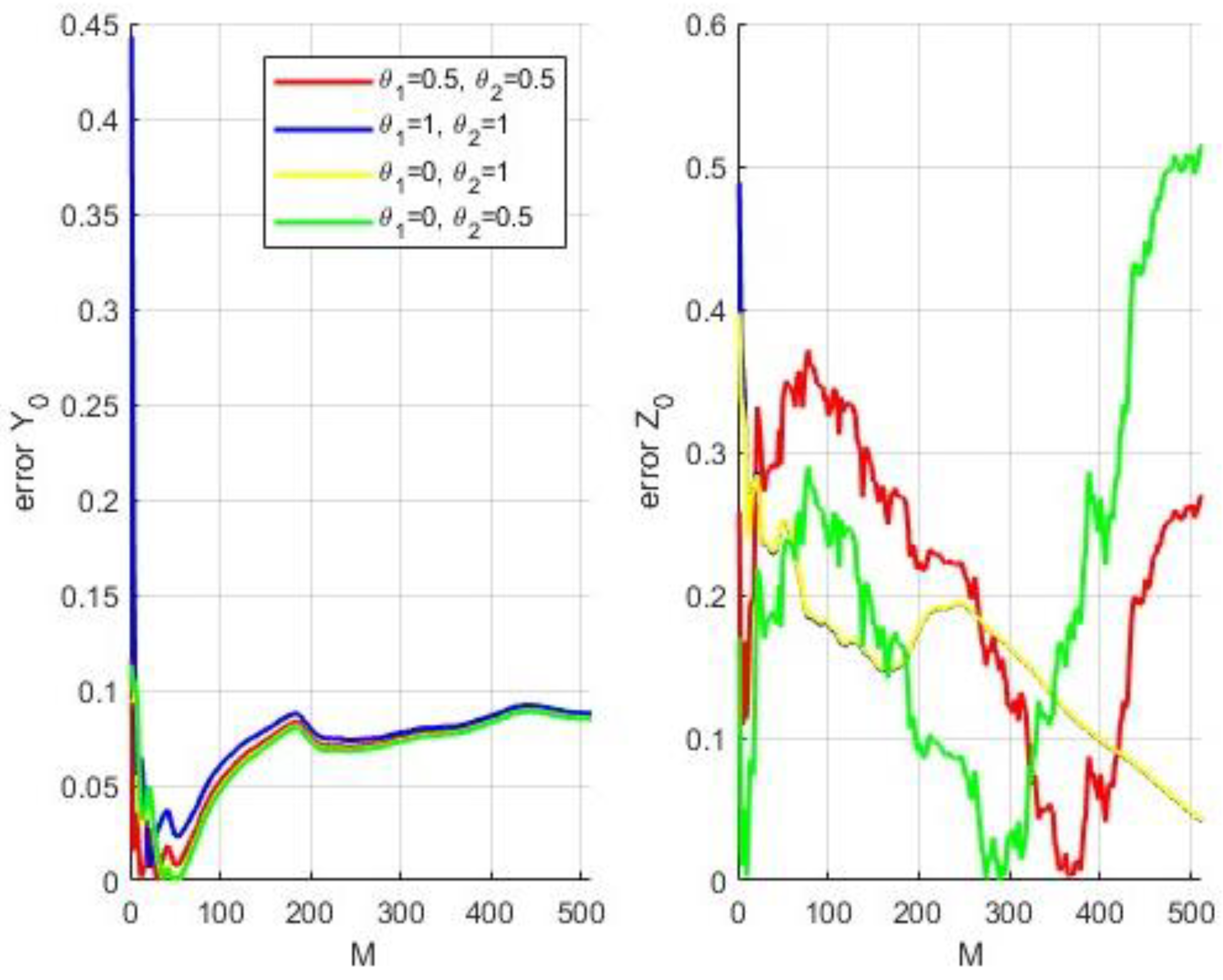
The results for the explicit algorithm, the local algorithm, and the global algorithm can be found separately in
Figure 10,
Figure 11 and
Figure 12. For
, we observe that the effects of the three algorithms do not differ significantly. Although the error from the figures increases when
, they converge at a certain number. For
, scheme B and scheme C are obviously smoother than other schemes. Interestingly, all schemes are smooth, and the error converges to a number for the explicit algorithm. For the local and global algorithms, the error has local oscillations, and their results are not as accurate as those of scheme B and scheme C.
Table 5 shows the CPU times for the explicit, local, and global algorithms. Since the time of each scheme (B, C, and D) in the same algorithm is approaching, only the case of scheme A is shown. Here, we also observe that the explicit algorithm is obviously faster than others. The CPU speeds of the local algorithm and the global algorithm are close.
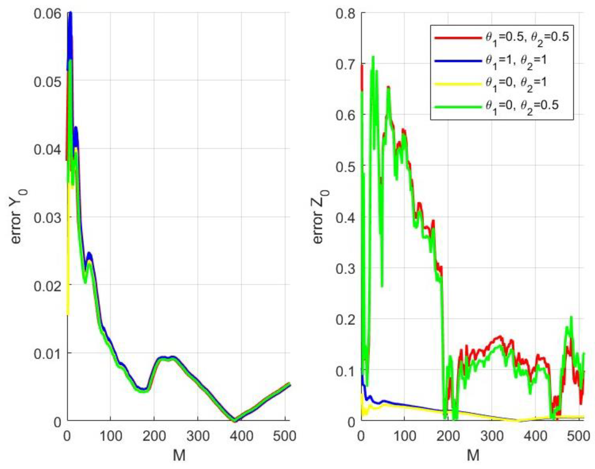
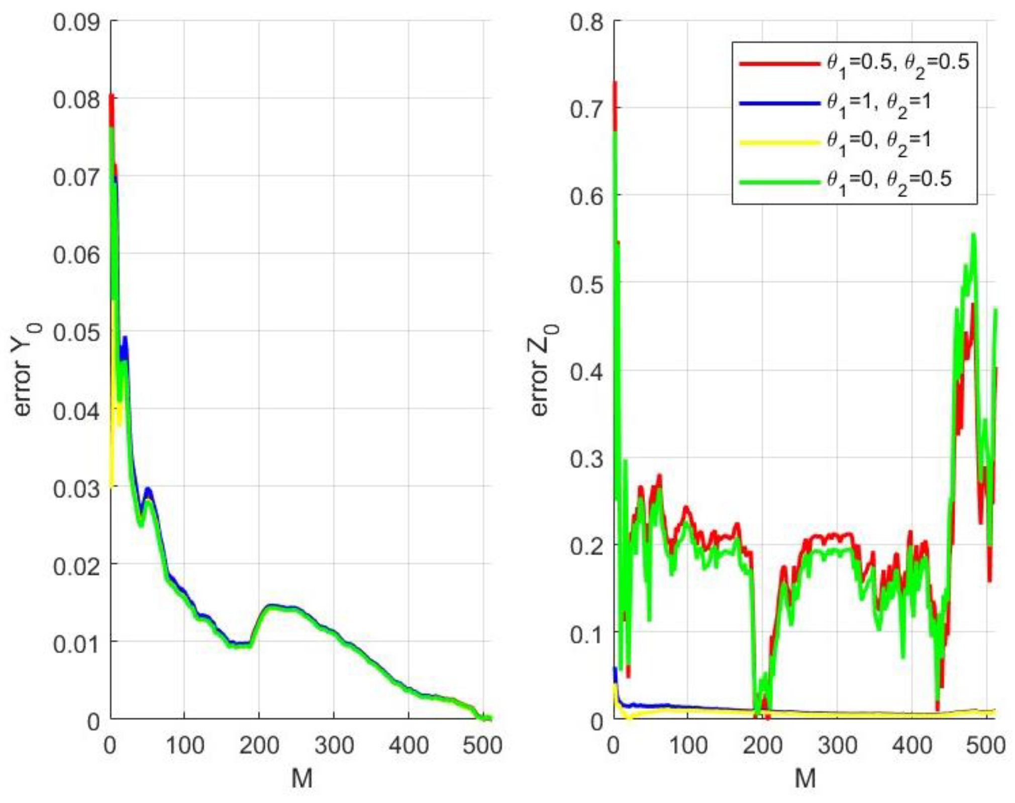
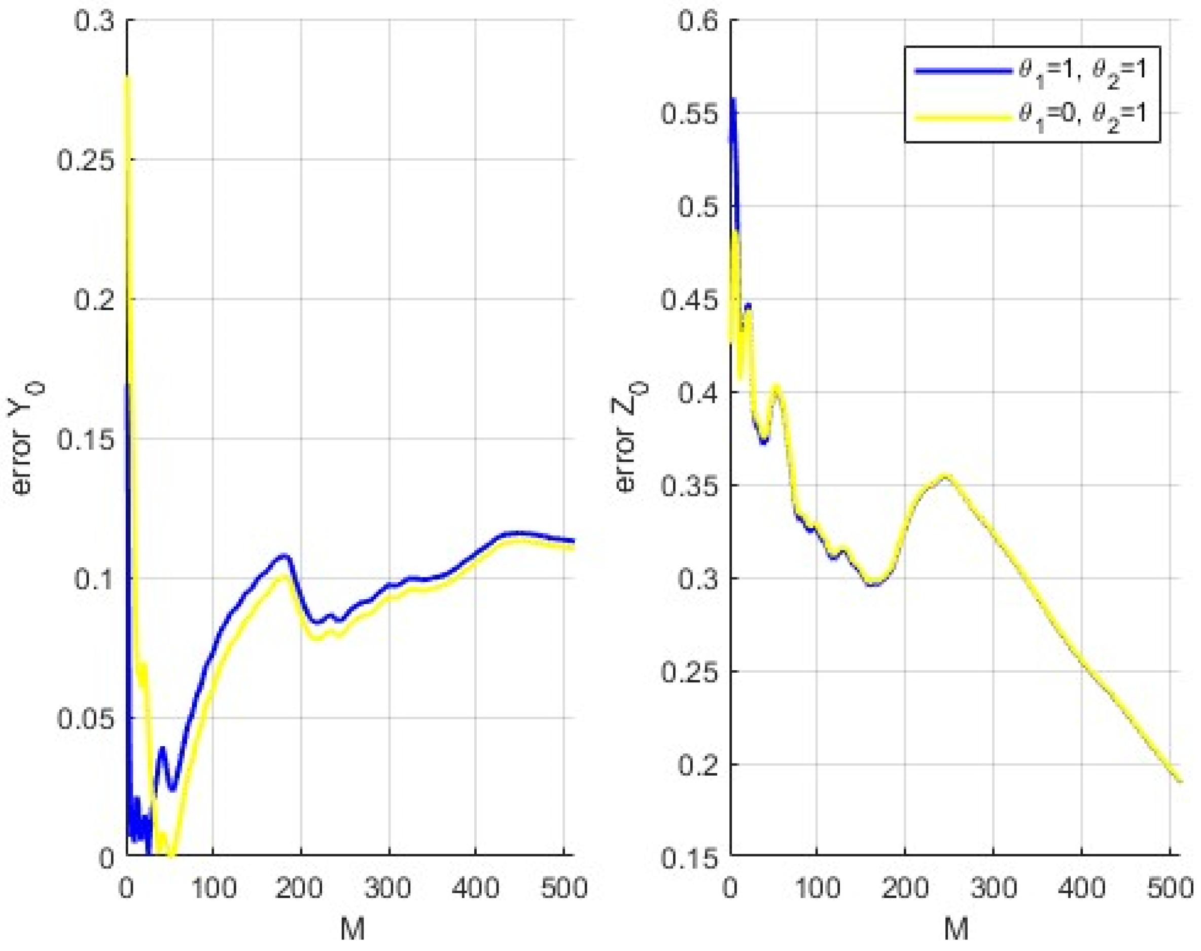
5.6. Example 6: Diffusion Depending on Zt
We consider the following coupled FBSDE:
where
This FBSDE satisfies assumptions (1)~(4). The solution of Equation (58) is given by:
For the experiment, we use and and set and . It is known that the exact solution is .
As the diffusion coefficient now depends on the process
, the nonlinear Feynman-Kac theorem is not applied. Therefore, we take scheme B and C in the first time step for the local algorithm and the global algorithm. The results for the three algorithms can be found separately in
Figure 13,
Figure 14 and
Figure 15. For
in the explicit algorithm, we observe that all schemes converge and that the effect of the local algorithm is better than those of the explicit and global methods. For
, scheme B and scheme C are smoother than other schemes in the explicit algorithm. Scheme A and scheme D are undulant. However, the approximations of
using the local and global methods have a divergent tendency. Their precision needs to be improved.
Table 6 shows the CPU times for the explicit, local, and global algorithms. The speed of all algorithms is still relatively great.
6. Conclusions
In this paper, based on three different numerical algorithms, we extend the fractional Fourier fast transform to propose methods for the numerical solution of multi-dimensional coupled FBSDEs. In this method, we prove a theorem in which the complicated conditional expectation containing Brown motion can be switched to expectation with time points and simple information. In order to verify the validity, we give three algorithms: the explicit algorithm, the local algorithm, and the global algorithm. Some examples show that the explicit algorithm performs best over the local and global algorithms because it is the fastest and most accurate. The calculated cost of this paper is cheaper than that of the case without FrFFT. The cost of the algorithms for the local algorithm and the global algorithm is more expensive than that of the explicit algorithm. However, the results of the local algorithm and the global algorithm are better than those of the explicit algorithm, especially in the case of example 2 (i.e., forward process depending on ). In a word, in the case of diffusion depending on , the accuracy of the numerical simulation of value of must be improved.
In future research, the case of diffusion depending on should be considered to improve accuracy, e.g., using Richardson extrapolation to accelerate the speed of convergence. In addition, FBSDEs with jumps can also be considered by applying the Fourier transform.
Author Contributions
Conceptualization, X.Z. and W.F.; formal analysis, J.D. and W.F.; funding acquisition, X.L.; methodology, X.L., X.Z. and K.F.; supervision, X.L.; writing original draft, X.Z.; writing—review and editing, J.D. All authors have read and agreed to the published version of the manuscript.
Funding
The authors were financially supported by the National Natural Science Foundation of China (62076039), Natural Science Foundation of Hubei Province (2022CFB023), Education Science Planning Project of Hubei Province (2022GA031), and college student innovation & entrepreneurship project from Yangtze University (Yz2022293).
Institutional Review Board Statement
Not applicable.
Informed Consent Statement
Not applicable.
Data Availability Statement
Not applicable.
Acknowledgments
We would like to express our thanks to the editors and the reviewers for their help.
Conflicts of Interest
The authors declare no conflict of interest.
References
- Pardoux, E.; Peng, S. Adapted solution of a backward stochastic differential equation. Syst. Control Lett. 1990, 14, 55–61. [Google Scholar] [CrossRef]
- Nam, K.; Xu, Y. Forward-backward stochastic equations: A functional fixed point approach. Stoch. Anal. Appl. 2023, 41, 16–44. [Google Scholar] [CrossRef]
- Yu, Z. On Forward-Backward Stochastic Differential Equations in a Domination-Monotonicity Framework. Appl. Math. Optim. 2022, 85, 1–46. [Google Scholar] [CrossRef]
- Douglas, J., Jr.; Ma, J.; Protter, P. Numerical methods for forward-backward stochastic differential equations. Ann. Appl. Probab. 1996, 6, 940–968. [Google Scholar] [CrossRef]
- Ma, J.; Shen, J.; Zhao, Y. On numerical approximations of forward-backward stochastic differential equations. SIAM J. Numer. Anal. 2008, 46, 2636–2661. [Google Scholar] [CrossRef]
- Millet, A.; Morien, P.L. On implicit and explicit discretization schemes for parabolic SPDEs in any dimension. Stoch. Process. Appl. 2005, 115, 1073–1106. [Google Scholar] [CrossRef]
- Ge, Y.; Li, L.; Zhang, G. A Fourier Transform Method for Solving Backward Stochastic Differential Equations. Methodol. Comput. Appl. Probab. 2022, 24, 385–412. [Google Scholar] [CrossRef]
- Li, X.; Wu, Y.; Zhu, Q.; Hu, S.; Qin, C. A regression-based Monte Carlo method to solve two-dimensional forward backward stochastic differential equations. Adv. Differ. Equ. 2021, 2021, 1–13. [Google Scholar] [CrossRef]
- Meng, Q.J.; Ding, D. An efficient pricing method for rainbow options based on two-dimensional modified sine-sine series expansions. Int. J. Comput. Math. 2013, 90, 1096–1113. [Google Scholar] [CrossRef]
- Ruijter, M.J.; Oosterlee, C.W.; Aalbers, R.F.T. On the Fourier cosine series expansion method for stochastic control problems. Numer. Linear Algebra Appl. 2013, 20, 598–625. [Google Scholar] [CrossRef]
- Crisan, D.; Manolarakis, K. Second order discretization of backward SDEs and simulation with the cubature method. Ann. Appl. Probab. 2014, 24, 652–678. [Google Scholar] [CrossRef]
- Li, H.; Xu, J.; Zhang, H. Solution to forward-backward stochastic differential equations with random coefficients and application to deterministic optimal control. IEEE Trans. Autom. Control 2022, 67, 6888–6895. [Google Scholar] [CrossRef]
- Zhao, W.; Wang, J.; Peng, S. Error estimates of the θ-scheme for backward stochastic differential equations. Discret. Contin. Dyn. Syst.-B 2009, 12, 905. [Google Scholar] [CrossRef]
- Zhao, W.; Li, Y.; Zhang, G. A generalized θ-scheme for solving backward stochastic differential equations. Discret. Contin. Dyn. Syst.-B 2012, 17, 1585. [Google Scholar] [CrossRef]
- Zhao, W.; Zhang, W.; Ju, L. A numerical method and its error estimates for the decoupled forward-backward stochastic differential equations. Commun. Comput. Phys. 2014, 15, 618–646. [Google Scholar] [CrossRef]
- Bender, C.; Zhang, J. Time discretization and Markovian iteration for coupled FBSDEs. Ann. Appl. Probab. 2008, 18, 143–177. [Google Scholar] [CrossRef]
- Zhao, W.; Fu, Y.; Zhou, T. New kinds of high-order multistep schemes for coupled forward backward stochastic differential equations. SIAM J. Sci. Comput. 2014, 36, A1731–A1751. [Google Scholar] [CrossRef]
- Huijskens, T.P.; Ruijter, M.J.; Oosterlee, C.W. Efficient numerical Fourier methods for coupled forwardbackward SDEs. J. Comput. Appl. Math. 2016, 296, 593–612. [Google Scholar] [CrossRef]
- Nam, K.; Xu, Y. Coupled FBSDEs with measurable coefficients and its application to parabolic PDEs. J. Math. Anal. Appl. 2022, 151, 126403. [Google Scholar] [CrossRef]
- Han, J.; Jentzen, A. Deep learning-based numerical methods for high-dimensional parabolic partial differential equations and backward stochastic differential equations. Commun. Math. Stat. 2017, 5, 349–380. [Google Scholar]
- Han, J.; Long, J. Convergence of the deep BSDE method for coupled FBSDEs. Probab. Uncertain. Quant. Risk 2020, 5, 1–33. [Google Scholar] [CrossRef]
- Ji, S.; Peng, S.; Peng, Y.; Zhang, X. Three algorithms for solving high-dimensional fully coupled FBSDEs through deep learning. IEEE Intell. Syst. 2020, 35, 71–84. [Google Scholar] [CrossRef]
- Zhao, W.; Chen, L.; Peng, S. A new kind of accurate numerical method for backward stochastic differential equations. SIAM J. Sci. Comput. 2006, 28, 1563–1581. [Google Scholar] [CrossRef]
- El Karoui, N.; Peng, S.; Quenez, M.C. Backward stochastic differential equations in finance. Math. Finance 1997, 7, 1–71. [Google Scholar] [CrossRef]
- Pham, H. Continuous-Time Stochastic Control and Optimization with Financial Applications; Springer Science & Business Media: Berlin/Heidelberg, Germany, 2009. [Google Scholar]
- Pardoux, E.; Tang, S. Forward-backward stochastic differential equations and quasilinear parabolic PDEs. Probab. Theory Relat. Fields 1999, 114, 123–150. [Google Scholar] [CrossRef]
- Bailey, D.H.; Swarztrauber, P.N. The fractional Fourier transform and applications. SIAM Rev. 1991, 33, 389–404. [Google Scholar] [CrossRef]
- Bayraktar, E.; Xing, H. Pricing American options for jump diffusions by iterating optimal stopping problems for diffusions. Math. Methods Oper. Res. 2009, 70, 505–525. [Google Scholar] [CrossRef]
- Chen, J.; Fan, L.; Li, L.; Zhang, G. Sinc Approximation of Multidimensional Hilbert Transform and Its Applications. SSRN 3091664. 2021. Available online: https://papers.ssrn.com/sol3/papers.cfm?abstract_id=3091664 (accessed on 24 May 2023).
- Delarue, F.; Menozzi, S. A forward-backward stochastic algorithm for quasi-linear PDEs. Ann. Appl. Probab. 2006, 16, 140–184. [Google Scholar] [CrossRef]
- Hyndman, C.B.; Ngou, P.O. Global convergence and stability of a convolution method for numerical solution of BSDEs. arXiv 2014, arXiv:1410.8595. [Google Scholar]
Figure 1.
Plot of the error of the example 1.
Figure 1.
Plot of the error of the example 1.
Figure 2.
Plot of the error of the explicit algorithm for example 2.
Figure 2.
Plot of the error of the explicit algorithm for example 2.
Figure 3.
Plot of the error of the local algorithm for example 2.
Figure 3.
Plot of the error of the local algorithm for example 2.
Figure 4.
Plot of the error of the explicit algorithm for example 3.
Figure 4.
Plot of the error of the explicit algorithm for example 3.
Figure 5.
Plot of the error of the local algorithm for example 3.
Figure 5.
Plot of the error of the local algorithm for example 3.
Figure 6.
Plot of the error of the global algorithm for example 3.
Figure 6.
Plot of the error of the global algorithm for example 3.
Figure 7.
Plot of the error of the explicit algorithm for example 4.
Figure 7.
Plot of the error of the explicit algorithm for example 4.
Figure 8.
Plot of the error of the local algorithm for example 4.
Figure 8.
Plot of the error of the local algorithm for example 4.
Figure 9.
Plot of the error of the global algorithm for example 4.
Figure 9.
Plot of the error of the global algorithm for example 4.
Figure 10.
Plot of the error of the explicit algorithm for example 5.
Figure 10.
Plot of the error of the explicit algorithm for example 5.
Figure 11.
Plot of the error of the local algorithm for example 5.
Figure 11.
Plot of the error of the local algorithm for example 5.
Figure 12.
Plot of the error of the global algorithm for example 5.
Figure 12.
Plot of the error of the global algorithm for example 5.
Figure 13.
Plot of the error of the explicit algorithm for example 6.
Figure 13.
Plot of the error of the explicit algorithm for example 6.
Figure 14.
Plot of the error of the local algorithm for example 6.
Figure 14.
Plot of the error of the local algorithm for example 6.
Figure 15.
Plot of the error of the global algorithm for example 6.
Figure 15.
Plot of the error of the global algorithm for example 6.
Table 1.
Error of results (, ) for example 1 by scheme A.
Table 1.
Error of results (, ) for example 1 by scheme A.
| Error | | Time (s) | | Time (s) | | Time (s) |
|---|
| 4 | | | 0.010592 | | 0.02287 | | 0.024719 |
| 3 | | | | | |
| 8 | | 5 | 0.019609 | | 0.034164 | | 0.041977 |
| | | | | | |
| 16 | | | 0.03041 | | 0.062138 | | 0.065344 |
| | | | | | |
| 32 | | | 0.060005 | | 0.100117 | | 0.128925 |
| | | | | | |
| 64 | | | 0.099635 | | 0.218806 | | 0.266788 |
| | | | | | |
| 128 | | | 0.243116 | | 0.447437 | | 0.584943 |
| | | | | | |
| 256 | | | 0.530708 | | 1.006999 | | 1.499762 |
| | | | | | |
| 512 | | | 1.455568 | | 2.657796 | | 3.964449 |
| | | | | | |
Table 2.
Error of results (, ) for example 2 by scheme C.
Table 2.
Error of results (, ) for example 2 by scheme C.
| Error | | Time (s) | | Time (s) | | Time (s) |
|---|
| 4 | | | 0.005422 | | 0.008908 | | 0.019683 |
| | | | | | |
| 8 | | | 0.009573 | | 0.016703 | | 0.032749 |
| | | | | | |
| 16 | | | 0.025286 | | 0.028508 | | 0.052708 |
| | | | | | |
| 32 | | | 0.04016 | | 0.05021 | | 0.097333 |
| | | | | | |
| 64 | | | 0.077589 | | 0.099154 | | 0.207257 |
| | | | | | |
| 128 | | | 0.159869 | | 0.20815 | | 0.432267 |
| | | | | | |
| 256 | | | 0.325549 | | 0.463633 | | 0.982044 |
| | | | | | |
| 512 | | | 0.759207 | | 1.156449 | | 2.491836 |
| | | | | | |
Table 3.
CPU times of scheme A for example 3(s).
Table 3.
CPU times of scheme A for example 3(s).
| 4 | 8 | 16 | 32 | 64 | 128 | 256 | 512 |
|---|
| Explicit | 0.012533 | 0.025716 | 0.035425 | 0.066304 | 0.155958 | 0.283224 | 0.613946 | 1.558809 |
| Local | 0.043708 | 0.070042 | 0.104299 | 0.227083 | 0.442085 | 0.909928 | 2.054779 | 4.157252 |
| Global | 0.052723 | 0.090697 | 0.182892 | 0.326598 | 0.623499 | 1.280217 | 2.141616 | 4.563165 |
Table 4.
CPU times of scheme A for example 4 (s).
Table 4.
CPU times of scheme A for example 4 (s).
| 4 | 8 | 16 | 32 | 64 | 128 | 256 | 512 |
|---|
| Explicit | 0.009843 | 0.021973 | 0.035312 | 0.061192 | 0.125936 | 0.271638 | 0.629419 | 1.451987 |
| Local | 0.065195 | 0.105617 | 0.202525 | 0.326405 | 0.538356 | 1.148581 | 2.342291 | 6.382512 |
| Global | 0.080436 | 0.170601 | 0.310428 | 0.518835 | 0.794979 | 1.540419 | 3.223398 | 8.397285 |
Table 5.
CPU times of scheme A for the example 5 (s).
Table 5.
CPU times of scheme A for the example 5 (s).
| 4 | 8 | 16 | 32 | 64 | 128 | 256 | 512 |
|---|
| Explicit | 0.009185 | 0.016861 | 0.028855 | 0.051736 | 0.097597 | 0.209269 | 0.503181 | 1.276852 |
| Local | 0.037164 | 0.054169 | 0.090534 | 0.175027 | 0.339829 | 0.720882 | 1.554783 | 4.157505 |
| Global | 0.049146 | 0.079958 | 0.160758 | 0.280679 | 0.526248 | 1.199261 | 2.558428 | 5.285499 |
Table 6.
CPU times of scheme B for example 6 (s).
Table 6.
CPU times of scheme B for example 6 (s).
| 4 | 8 | 16 | 32 | 64 | 128 | 256 | 512 |
|---|
| Explicit | 0.007739 | 0.012715 | 0.024707 | 0.039612 | 0.077765 | 0.187745 | 0.405907 | 1.122424 |
| Local | 0.066662 | 0.106036 | 0.210299 | 0.403093 | 0.815283 | 1.855567 | 4.125572 | 11.050587 |
| Global | 0.089035 | 0.201116 | 0.334744 | 0.673482 | 1.176203 | 2.425878 | 4.909738 | 10.333279 |
| Disclaimer/Publisher’s Note: The statements, opinions and data contained in all publications are solely those of the individual author(s) and contributor(s) and not of MDPI and/or the editor(s). MDPI and/or the editor(s) disclaim responsibility for any injury to people or property resulting from any ideas, methods, instructions or products referred to in the content. |
© 2023 by the authors. Licensee MDPI, Basel, Switzerland. This article is an open access article distributed under the terms and conditions of the Creative Commons Attribution (CC BY) license (https://creativecommons.org/licenses/by/4.0/).


