Stability and Bifurcation Analysis of Fifth-Order Nonlinear Fractional Difference Equation

Abstract

In this paper, a rational difference equation with positive parameters and non-negative conditions is used to determine the presence and direction of the Neimark–Sacker bifurcation. The neimark–Sacker bifurcation of the system is first studied using the characteristic equation. In addition, we study bifurcation invariant curves from the perspective of normal form theory. A computer simulation is used to illustrate the analytical results.

1. Introduction

1.1. Motivation and Literature Review

In many fields, including economics, biology, and physics, difference equations are essential. Therefore, this field of research is attracting an increasing number of researchers. Since rational difference equations are closed forms of nonlinear difference equations, there is a lot of research on their qualitative behavior. Camouzis et al. [1] present an analysis of the local stability of the rational difference equation at its positive equilibrium point.

$$c_{n+1}=\frac{\varsigma c_{n-2}+c_{n-3}}{p+c_{n-3}}$$

(1)

$\varsigma$ and p have positive values and the initial conditions are non-negative. In addition, the authors proved that the positive equilibrium point is locally stable if ${\varsigma }^3+{\varsigma }^2-(2p^2+4p+2)\varsigma p^3+p^2-p-1<0$ and unstable if ${\varsigma }^3+{\varsigma }^2-(2p^2+4p+2)\varsigma +p^3+p^2-p-1>0$, additionally, if $p-1<\varsigma \le p+1$, then every positive solution of Equation (1) converges to the positive fixed point.

Zhang and Ding [2] studied the existence and direction of Neimark–Sacker bifurcation of Equation (1). The authors proved that if $\varsigma >p-1$ and if $\varsigma$ satisfies ${\varsigma }^3+{\varsigma }^2-(2p^2+4p+2)\varsigma +p^3+p^2-p-1=0$ then Neimark–Sacker bifurcation occurs.

Camouzis [3] examined the global nature of the third order rational difference equation

$$c_{n+1}=\frac{\varsigma c_n+\partial c_{n-2}}{p+Q{c}_n+R{c}_{n-1}}$$

(2)

where the parameters $\varsigma ,\partial ,p$ are non-negative $\varsigma +\partial >0,Q,R>0$ and the initial values $c_{-2},c_{-1},c_0$ are non-negative real numbers. Using a suitable modification in the variables,

$$c_{n+1}=\frac{\varsigma c_n+c_{n-2}}{p+Q{x}_n+c_{n-1}}$$

(3)

where $p\ge 0,\varsigma >0,Q>0$. The author focused on examining the boundness of solutions of Equation (3). Along the same lines of research, authors in [4] examined whether the third order difference equation has a Neimark–Sacker bifurcation.

$$c_{n+1}=\frac{\varsigma c_n+\alpha c_{n-2}}{1+c_{n-1}}$$

(4)

With parameters $\alpha$, $\varsigma$$ϵ$(0, ∞) and initial conditions $c_{-2},c_{-1},c_0$ that are non-negative. It has been shown in Camouzis and Ladas [5] that the unique positive equilibrium $c^{*}=\alpha +\varsigma -1$, $\alpha +\varsigma$$>1$ is locally asymptotically stable when $\varsigma >{\varsigma }^{*}$ and unstable when $\varsigma <{\varsigma }^{*}$ where ${\varsigma }^{*}=({\alpha }^2-\alpha )/(\alpha +1)$. The authors in [4] proved the existence of Neimark–Sacker bifurcation for Equation (4) as $\varsigma$ passes through the critical value ${\varsigma }^{*}$.

In [6] Shareef and Aloqeili studied Neimark–Sacker bifurcation of the following rational difference equation

$$c_{n+1}=\frac{\varsigma c_n+c_{n-3}}{p+c_{n-1}}$$

(5)

where the parameters and the initial conditions are non-negative.

In [7], the authors studied the global dynamics and bifurcations of the following two quadratic fractional second-order difference equations:

$$c_{n+1}=\frac{\varsigma c_n+c_{n-1}+\gamma c_{n-1}}{p{c}_n^2+Q{c}_n{c}_{n-1}}$$

(6)

In [8], rusticet et al. investigated the global dynamics and bifurcations of certain second-order rational difference equation with quadratic terms of the following form

$$c_{n+1}=\frac{c_{n-1}}{p{x}_n^2+q{c}_{n-1}+r}$$

(7)

Recently, in [9], Kulenovic et al. studied the Neimark–Sacker bifurcation of the following second-order rational difference equation with quadratic terms

$$c_{n+1}=\frac{R}{p{c}_n{c}_{n-1}+q{c}_{n-1}^2+r}$$

(8)

Considering the rational difference equation of the fifth order is motivated by the above work

$$c_{n+1}=\frac{\varsigma c_n+c_{n-4}}{p+c_{n-1}}$$

(9)

with positive parameters $\varsigma$ and p and non-negative initial conditions $c_{-4},c_{-3},c_{-2},c_{-1},c_0$.

Camouzis and Ladas in [1] have conjectured that the difference equation

$$c_{n+1}=\frac{\varsigma c_n+\gamma c_{n-3}}{p+Q{c}_{n-1}}$$

(10)

for some parameters and initial conditions, it has unbounded solutions. This paper will not prove this conjecture. Equation (9) is a special case of $\gamma =Q=1$ in the previous equation. Numerical simulations showed that for the range of parameter $p<p*$ in Figure 1, the solution of Equation (9) is unbounded. As a result, there is no parabolic shape near the bifurcation value. As you can see in Equation (1), $c_{n+1}$ is based solely on $c_{n-2}$ and $c_{n-3}$, but in Equation (9), $c_{n+1}$ is dependent on $c_n$, $c_{n-1}$, and $c_{n-4}$. To prove the existence of the Neimark–Sacker bifurcation, the same steps are used, including demonstrating that a complex conjugate pair of modulus one eigenvalues exists as well as studying the direction of the bifurcation. However, the calculations differ. Similar equations can be studied using the details of the calculations. A positive equilibrium $c^{*}=\alpha +\varsigma -1$, is formed when $\varsigma +1>p$ for Equation (9). The next section examines the local stability of this equilibrium. We then demonstrate that this equation undergoes Neimark–Sacker bifurcation when p crosses a certain critical value $p*$. Next, we study the direction of the bifurcation. Finally, we present some numerical simulations that support our theoretical analysis. As a discrete time population model, difference equations have a long history [10]. In most cases, these equations describe autonomous, discrete-time dynamics and assume that the only temporal change in vital rates is due to population density (thereby leading to nonlinear difference equations). Vital rates, however, are affected by a variety of other mechanisms and circumstances. In addition, the population’s physical and biological environment can fluctuate, either systematically (such as daily, monthly, or seasonal changes) or randomly (such as stochastic weather fluctuations, resource availability, etc.). For more results, we refer to [11,12,13,14,15,16,17,18,19,20,21].

1.2. Structure of the Paper

The structure of this paper will be as follows: In the following section, we will examine the fixed points along with a linearized form of Equation (11) and apply the jury conditions to evaluate the stability of the system. In Theorem 3, we examined the periodic solution of the model (11). In Section 3 we studied the existence and direction of the Neimark–Sacker bifurcation. The theoretical results are numerically verified in Section 4, whereas the conclusion of the paper is given in Section 5.

2. Main Results

Dynamics of $c_{n+1}=\frac{\varsigma c_n+c_{n-4}}{p+c_{n-1}}$

In this section, we study stability and bifurcation analysis rational difference equation of fifth order

$$c_{n+1}=\frac{\varsigma c_n+c_{n-4}}{p+c_{n-1}}$$

(11)

with positive $\varsigma$ and p parameters and non-negative initial condition $c_0,c_{-1},c_{-2},$ $c_{-3},c_{-4}$, finding equilibrium points of (11)

$$g(\overline{c},\overline{c},\overline{c},\overline{c})=\overline{c}$$

so

$$c^{*}=\frac{(\varsigma +1)c^{*}}{p+c^{*}}$$

$$c^{*}(p+c^{*})=(\varsigma +1)c^{*}$$

$$c^{*}(p+c^{*})-(\varsigma +1)c^{*}=0$$

So, it contain two fixed points,

$$\begin{array}{c}{c}^{*}(0,0,0,0,0)and{c}^{*}=(\varsigma -p+1,\varsigma -p+1,\varsigma -p+1,\varsigma -p+1)\hfill \end{array}$$

When $\varsigma +1>p$ having a unique positive fixed points, let $\varsigma +1>p$.

Suppose

$$\left(\begin{array}{c}{u}_n\hfill \\ v_n\hfill \\ w_n\hfill \\ z_n\hfill \\ t_n\hfill \end{array}\right)=\left(\begin{array}{c}{c}_n\hfill \\ c_{n-1}\hfill \\ c_{n-2}\hfill \\ c_{n-3}\hfill \\ c_{n-4}\hfill \end{array}\right)$$

So its change into

$$\left(\begin{array}{c}{u}_{n+1}\hfill \\ v_{n+1}\hfill \\ w_{n+1}\hfill \\ z_{n+1}\hfill \\ t_{n+1}\hfill \end{array}\right)=\left(\begin{array}{c}\frac{\varsigma u_n+t_n}{p+u_n}\hfill \\ u_n\hfill \\ v_n\hfill \\ w_n\hfill \\ z_n\hfill \end{array}\right)$$

(12)

Theorem 1.

Positive fixed point is stable at $\varsigma >{\varsigma }^{*}$, and unstable at $\varsigma <{\varsigma }^{*}$, where

$${\varsigma }^{*}=\frac{5p^2+13p+6}{p+1}$$

Proof. 

(12) has a Jacobian matrix

$$S\left(\eta \right)=\left|\begin{array}{ccccc}\frac{\varsigma }{\varsigma +1}\hfill & -\left(\frac{\varsigma -p+1}{\varsigma +1}\right)& 0\hfill & 0& \frac{1}{\varsigma +1}\\ 1\hfill & 0& 0\hfill & 0& 0\\ 0\hfill & 1& 0\hfill & 0& 0\\ 0\hfill & 0& 1\hfill & 0& 0\\ 0\hfill & 0& 0\hfill & 1& 0\end{array}\right|$$

The characteristic equation’s Jacobean matrix is

$S\left(\eta \right)=\left|\mathrm{J}-\eta I\right|$

$$S\left(\eta \right)=\left|\begin{array}{ccccc}\frac{\varsigma }{\varsigma +1}-\eta \hfill & \frac{-(\varsigma -p+1)}{\varsigma +1}& 0\hfill & 0& \frac{1}{\varsigma +1}\\ 1\hfill & -\eta & 0\hfill & 0& 0\\ 0\hfill & 1& -\eta \hfill & 0& 0\\ 0\hfill & 0& 1\hfill & -\eta & 0\\ 0\hfill & 0& 0\hfill & 1& -\eta \end{array}\right|$$

$$S\left(\eta \right)=(\frac{\varsigma }{\varsigma +1}-\eta ){(-\eta )}^4+\left(\frac{\varsigma -p+1}{\varsigma +1}\right){(-\eta )}^3+\frac{1}{\varsigma +1}$$

$$S\left(\eta \right)=(\frac{\varsigma }{\varsigma +1}-\eta ){\eta }^4+\left(\frac{\varsigma -p+1}{\varsigma +1}\right){(-\eta )}^3+\frac{1}{\varsigma +1}$$

$$S\left(\eta \right)=-{\eta }^5+\frac{\varsigma }{\varsigma +1}{\eta }^4-\frac{\varsigma -p+1}{\varsigma +1}{\eta }^3+\frac{1}{\varsigma +1}$$

Let

$$S\left(\eta \right)=-S\left(\eta \right)$$

$$S\left(\eta \right)={\eta }^5-\frac{\varsigma }{\varsigma +1}{\eta }^4+\frac{\varsigma -p+1}{\varsigma +1}\eta -\frac{1}{\varsigma +1}$$

(13)

The jury conditions are used to investigate the stability of $c^{*}$.

(1)

necessary condition.

(2)

sufficient condition.

□

Theorem 2.

Polynomial which is in the form of

$$S\left(t\right)=j_n{t}^n+j_{n-1}{t}^{n-1}+............+j_{1}t+j_0$$

For stability necessary conditions are:

$$S\left(1\right)>0and{(-1)}^{n}S(-1)>0$$

By forming table sufficient condition for stability is obtained by

$$\begin{array}{ccccccccc}\mathrm{rows}\hfill & t^0& t^1\hfill & t^2& \dots & t^{n-k}& \dots & t^{n-1}& t^n\\ 1\hfill & j_0& j_1\hfill & j_2& \dots & j_{n-k}& \dots & j_{n-1}& j_n\\ 2\hfill & j_n& j_{n-1}\hfill & j_{n-2}& \dots & j_k& \dots & j_1& j_0\\ 3\hfill & k_0& k_1\hfill & k_2& \dots & k_{n-k}& \dots & k_{n-1}\\ 4\hfill & k_{n-1}& k_{n-2}\hfill & k_{n-3}& \dots & k_k& \dots & k_0& \\ 6\hfill & l_{n-2}& l_{n-3}\hfill & \dots & \dots & & l_0& & \\ & ⋮& ⋮\hfill & ⋮& ⋮& ⋮& ⋮& \cdots & ⋮\\ 2n-5\hfill & m_0& m_1\hfill & m_2& m_3& & & \\ 2n-4\hfill & m_3& m_2\hfill & m_1& m_0& & \\ 2n-3\hfill & n_0& n_1\hfill & n_2& & \end{array}$$

Now general form of sufficient condition is, where

$$j_k=\left|\begin{array}{cc}{j}_0& j_{n-k}\\ j_n& j_k\end{array}\right|,l_k=\left|\begin{array}{cc}{k}_0& k_{n-1-k}\\ k_{n-1}& k_k\end{array}\right|,d_k=\left|\begin{array}{cc}{l}_0& l_{n-2-k}\\ l_{n-2}& l_k\end{array}\right|$$

For stability the sufficient conditions are given by

$$\left|j_0\right|>j_n,\left|k_0\right|>\left|k_{n-1}\right|,\left|l_0\right|>\left|l_{n-2}\right|.....\left|n_0\right|>\left|n_2\right|$$

Apply the necessary condition

(i)

$$\begin{array}{ccc}S\left(1\right)\hfill & =& {\left(1\right)}^5-\frac{\varsigma }{\varsigma +1}{\left(1\right)}^4+\frac{\varsigma -p+1}{\varsigma +1}-\frac{1}{\varsigma +1}\hfill \\ S\left(1\right)\hfill & =& 1-\frac{\varsigma }{\varsigma +1}+\frac{\varsigma -p+1}{\varsigma +1}-\frac{1}{\varsigma +1}\hfill \\ S\left(1\right)\hfill & =& \frac{\varsigma -p+1}{\varsigma +1}>0.\hfill \end{array}$$

(ii)

$${(-1)}^{5}S(-1)=(-1)\left[{(-1)}^5-\frac{\varsigma }{\varsigma +1}{(-1)}^4+\frac{\varsigma -p+1}{\varsigma +1}{(-1)}^3-\frac{1}{\varsigma +1}\right]$$

$$=-1-1-\frac{\varsigma -p+1}{\varsigma +1}$$

$$=2+\frac{\varsigma -p+1}{\varsigma +1}>0$$

Now the necessary conditions are satisfied, we now apply sufficient condition

$$S\left(\eta \right)={\eta }^5-\frac{\varsigma }{\varsigma +1}{\eta }^4+\frac{\varsigma -p+1}{\varsigma +1}\eta -\frac{1}{\varsigma +1}$$

$$j_0=-\frac{1}{\varsigma +1},j_1=\frac{\varsigma -p+1}{\varsigma +1},j_2=0,j_3=0,j_4=-\frac{\varsigma }{\varsigma +1},j_5=1$$

$$\left|j_5\right|>\left|j_0\right|,\left|k_0\right|>\left|k_4\right|,\left|l_0\right|>\left|l_3\right|,\left|d_0\right|>\left|d_2\right|$$

$$k_0=\left|\begin{array}{cc}{j}_0& j_5\\ j_5& j_0\end{array}\right|=\left|\begin{array}{cc}-\frac{1}{\varsigma +1}& 1\\ 1& -\frac{1}{\varsigma +1}\end{array}\right|=\frac{1}{{(\varsigma +1)}^2}-1=\frac{-{\varsigma }^2-2\varsigma }{{(\varsigma +1)}^2}$$

$$k_1=\left|\begin{array}{cc}{j}_0& j_4\\ j_5& j_1\end{array}\right|=\left|\begin{array}{cc}-\frac{1}{\varsigma +1}& -\frac{\varsigma }{\varsigma +1}\\ 1& \frac{\varsigma -p+1}{\varsigma +1}\end{array}\right|=\frac{-{\varsigma }^2+p-1}{{(\varsigma +1)}^2}$$

$$k_2=\left|\begin{array}{cc}{j}_0& j_3\\ j_5& j_2\end{array}\right|=\left|\begin{array}{cc}-\frac{1}{\varsigma +1}& 0\\ 1& 0\end{array}\right|=0$$

$$k_3=\left|\begin{array}{cc}{j}_0& j_2\\ j_5& j_3\end{array}\right|=\left|\begin{array}{cc}-\frac{1}{\varsigma +1}& 0\\ 1& 0\end{array}\right|=0$$

$$k_4=\left|\begin{array}{cc}{j}_0& j_1\\ j_5& j_4\end{array}\right|=\left|\begin{array}{cc}-\frac{1}{\varsigma +1}& \frac{\varsigma -p+1}{\varsigma +1}\\ 1& -\frac{\varsigma }{\varsigma +1}\end{array}\right|=-\frac{{\varsigma }^2+\varsigma p+\varsigma -p+1}{{(\varsigma +1)}^2}$$

$$l_0=\left|\begin{array}{cc}{k}_0\hfill & k_4\\ k_4\hfill & k_0\end{array}\right|$$

$$=\left|\begin{array}{cc}-\frac{{\varsigma }^2+2\varsigma }{{(\varsigma +1)}^2}\hfill & \frac{-({\varsigma }^2+\varsigma p+\varsigma -p+1)}{{(\varsigma +1)}^2}\\ -\frac{{\varsigma }^2+\varsigma p+\varsigma -p+1}{{(\varsigma +1)}^2}\hfill & -\frac{{\varsigma }^2+2\varsigma }{{(\varsigma +1)}^2}\end{array}\right|={\left[\frac{{\varsigma }^2+2\varsigma }{{(1+\varsigma )}^2}\right]}^2-{\left[\frac{{\varsigma }^2+\varsigma p+\varsigma -p+1}{{(\varsigma +1)}^2}\right]}^2$$

$$\begin{array}{c}{l}_0=\frac{2{\varsigma }^3+{\varsigma }^2-{\varsigma }^{3}p-{\varsigma }^2{p}^2-2\varsigma +p^2+2p-1}{{(\varsigma +1)}^4}\hfill \end{array}$$

$$l_1=\left|\begin{array}{cc}{k}_0\hfill & k_3\\ k_4\hfill & k_1\end{array}\right|=\left|\begin{array}{cc}-\frac{{\varsigma }^2+2\varsigma }{{(1+\varsigma )}^2}\hfill & 0\\ \frac{-({\varsigma }^2+\varsigma p+\varsigma -p+1)}{{(\varsigma +1)}^2}\hfill & -\frac{{\varsigma }^2-p+1}{{(\varsigma +1)}^2}\end{array}\right|$$

$$\begin{array}{c}{l}_1=\frac{{\varsigma }^4+2{\varsigma }^3+{\varsigma }^2-{\varsigma }^{2}p-2\varsigma p+2\varsigma }{{(1+\varsigma )}^4}\hfill \end{array}$$

$$l_2=\left|\begin{array}{cc}{k}_0\hfill & k_2\\ k_4\hfill & k_2\end{array}\right|=\left|\begin{array}{cc}-\frac{{\varsigma }^2+2\varsigma }{{(1+\varsigma )}^2}\hfill & 0\\ -\frac{{\varsigma }^2+\varsigma p+\varsigma -p+1}{{(\varsigma +1)}^2}\hfill & 0\end{array}\right|$$

$$\begin{array}{c}{l}_2=0\hfill \end{array}$$

$$l_{3=}\left|\begin{array}{cc}{k}_0\hfill & k_1\\ k_4\hfill & k_3\end{array}\right|=\left|\begin{array}{cc}-\frac{{\varsigma }^2+2\varsigma }{{(1+\varsigma )}^2}\hfill & -\frac{{\varsigma }^2-p+1}{{(1+\varsigma )}^2}\\ -\frac{{\varsigma }^2+\varsigma p+\varsigma -p+1}{{(\varsigma +1)}^2}\hfill & 0\end{array}\right|$$

$$l_3==-\frac{{\varsigma }^4+{\varsigma }^{3}p+{\varsigma }^3-2{\varsigma }^{2}p+\varsigma +2{\varsigma }^2-\varsigma p^2-p+1}{{(1+\varsigma )}^4}$$

Now check for sufficient condition

(i)

$$\left|j_5\right|>\left|j_0\right|$$

$$\left|1\right|>|-\frac{1}{\varsigma +1}|$$

$$1>\frac{1}{\varsigma +1}$$

(ii)

$$\left|k_0\right|>\left|k_4\right|$$

$$|-\frac{{\varsigma }^2+2\varsigma }{{(\varsigma +1)}^2}|>|-\frac{{\varsigma }^2+\varsigma p+\varsigma -p+1}{{(\varsigma +1)}^2}|$$

$$\frac{3\varsigma +\varsigma p+p-1}{{(1+\varsigma )}^2}>0$$

(iii)

$$\left|l_0\right|>\left|l_3\right|$$

$$\left|\frac{2{\varsigma }^3+{\varsigma }^2-{\varsigma }^{3}p-{\varsigma }^2{p}^2-2\varsigma +p^2+2p-1}{{(\varsigma +1)}^4}\right|>\left|-\frac{{\varsigma }^4+{\varsigma }^{3}p+{\varsigma }^3-2{\varsigma }^{2}p+\varsigma +2{\varsigma }^2-\varsigma p^2-p+1}{{(1+\varsigma )}^4}\right|$$

$$\frac{{\varsigma }^4-{\varsigma }^3-{\varsigma }^2+{\varsigma }^{3}p+{\varsigma }^2{p}^2+3\varsigma -3p-2{\varsigma }^{2}p-\varsigma p^2-p^2+2}{{(1+\varsigma )}^4}>0$$

Theorem 3.

The difference equation $c_{n+1}=\frac{\varsigma c_n+c_{n-4}}{p+c_{n-1}}$ has no solution of period 2.

Proof. 

Proof on contrary suppose it is period 2 solution i.e., ……$e,r,e,r$,……where $e\ne r$ then $e=\frac{\varsigma r+r}{p+e}$.

We have

$$r(\varsigma +1)=ep+e^2$$

(14)

and $r=\frac{\varsigma e+e}{p+q}$ so we have,

$$e(\varsigma +1)=rp+r^2$$

(15)

solving (14) and (15) these equation we get

$$(e-r)(p+e+r+\varsigma +1)=0.$$

But

$$(p+e+r+\varsigma +1)>0,$$

so, $(e-r)=0$ which implies $e=r$. Which completes the proof. □

3. Existence of Neimark-Sacker Bifurcation of ${\mathit{c}}_{\mathit{n}+\mathit{1}}=\frac{\mathit{\varsigma }{\mathit{c}}_{\mathit{n}}+{\mathit{c}}_{\mathit{n}-\mathit{4}}}{\mathit{p}+{\mathit{c}}_{\mathit{n}-\mathit{1}}}$

In this section, we will look at the Neimark–Sacker bifurcation of (11) which occurs at $p=p^{*}$ as p is bifurcation parameter. Note that Equation (11) has no positive prime period two solution. Hence, we focus our attention on Neimark–Sacker bifurcaton

Theorem 4

([13] (Viete formula)). For any general degree n

$$f\left(t\right)=j_n{t}^n+j_{n-1}{t}^{n-1}+...+j_{1}t+j_0$$

The polynomial coefficient $a_k$ is related to the signed sum by the Viete formula. The following are the products of its roots  $t_{i,i=1,2,\dots }$

$$t_1+t_2+\dots t_{n-1}+t_n=\frac{-j_n-1}{j_n}$$

$$(t_1{t}_2+t_1{t}_3+\dots +t_1{t}_n)+(t_2{t}_2+t_2{t}_3+\dots +t_2{t}_n)+\dots t_{n-1}{t}_n=\frac{j_{n-2}}{j_n}$$

$$t_1{t}_2\dots t_n={(-1)}^n\frac{j_0}{j_n}$$

Proof. 

Proof suppose that ${\eta }_1,{\eta }_2,{\eta }_3,{\eta }_4,{\eta }_5$ are the roots of (4.1.1) where ${\eta }_1={\eta }_2$ and ${\eta }_3=\varsigma$ by viete theorem by polynomial

$$S\left(\eta \right)={\eta }^5-\frac{\varsigma }{\varsigma +1}{\eta }^4+\frac{\varsigma -p+1}{\varsigma +1}{\eta }^3-\frac{1}{\varsigma +1}$$

where $j_0=-\frac{1}{\varsigma +1},j_2=0,j_3=\frac{\varsigma -p+1}{\varsigma +1},j_4=-\frac{\varsigma }{\varsigma +1},j_5=1$ if $\left|{\eta }_1\right|=\left|{\eta }_2\right|=\left|{\eta }_3\right|=\left|{\eta }_4\right|=1$ and ${\eta }_5=\varsigma$, we obtain

$${\eta }_1+{\eta }_2+{\eta }_3+{\eta }_4+{\eta }_5=-\frac{j_4}{j_5}$$

(16)

$${\eta }_1{\eta }_2+{\eta }_1{\eta }_3+{\eta }_1{\eta }_4+{\eta }_1{\eta }_5+{\eta }_2{\eta }_3+{\eta }_2{\eta }_4+{\eta }_2{\eta }_5+{\eta }_3{\eta }_4+{\eta }_3{\eta }_5+{\eta }_4{\eta }_5=\frac{j_3}{j_5}$$

(17)

$${\eta }_1{\eta }_2{\eta }_3+{\eta }_1{\eta }_2{\eta }_4+{\eta }_1{\eta }_2{\eta }_5+{\eta }_1{\eta }_3{\eta }_4+{\eta }_1{\eta }_3{\eta }_5+{\eta }_1{\eta }_4{\eta }_5+{\eta }_2{\eta }_3{\eta }_4+{\eta }_2{\eta }_3{\eta }_5$$

$$+{\eta }_2{\eta }_4{\eta }_5+{\eta }_3{\eta }_4{\eta }_5=-\frac{j_2}{j_5}$$

(18)

$${\eta }_1{\eta }_2{\eta }_3{\eta }_4+{\eta }_{1‘}{\eta }_2{\eta }_3{\eta }_5+{\eta }_1{\eta }_3{\eta }_4{\eta }_5+{\eta }_2{\eta }_3{\eta }_4{\eta }_5=\frac{j_1}{j_5}$$

(19)

$${\eta }_1{\eta }_2{\eta }_3{\eta }_4{\eta }_5=-\frac{j_0}{j_5}$$

(20)

$${\eta }_1+{\eta }_2+{\eta }_3+{\eta }_4+{\eta }_5=-\frac{\varsigma }{\varsigma +1}$$

(21)

$${\eta }_1{\eta }_2+{\eta }_1{\eta }_3+{\eta }_1{\eta }_4+{\eta }_1{\eta }_5+{\eta }_2{\eta }_3$$

$$+{\eta }_2{\eta }_4+{\eta }_2{\eta }_5+{\eta }_3{\eta }_4+{\eta }_3{\eta }_5+{\eta }_4{\eta }_5=\frac{\varsigma -p+1}{\varsigma +1}$$

(22)

$${\eta }_1{\eta }_2{\eta }_3+{\eta }_1{\eta }_2{\eta }_4+{\eta }_1{\eta }_2{\eta }_5+{\eta }_1{\eta }_3{\eta }_4+{\eta }_1{\eta }_3{\eta }_5+{\eta }_1{\eta }_4{\eta }_5+{\eta }_2{\eta }_3{\eta }_4$$

$$+{\eta }_2{\eta }_3{\eta }_5+{\eta }_2{\eta }_4{\eta }_5+{\eta }_3{\eta }_4{\eta }_5=0$$

(23)

$${\eta }_1{\eta }_2{\eta }_3{\eta }_4+{\eta }_{1‘}{\eta }_2{\eta }_3{\eta }_5+{\eta }_1{\eta }_3{\eta }_4{\eta }_5+{\eta }_2{\eta }_3{\eta }_4{\eta }_5=0$$

(24)

$${\eta }_1{\eta }_2{\eta }_3{\eta }_4{\eta }_5=-\frac{1}{\varsigma +1}$$

(25)

$$\left|{\eta }_1\right|=\left|{\eta }_2\right|=\left|{\eta }_3\right|=\left|{\eta }_4\right|=1$$

$${\eta }_5=-\frac{1}{\varsigma +1}$$

(26)

$$1+1+1+1+1+1+({\eta }_1+{\eta }_2+{\eta }_3+{\eta }_4){\eta }_5=\frac{\varsigma -p+1}{\varsigma +1}$$

$${\eta }_1+{\eta }_2+{\eta }_3+{\eta }_4=7+5\varsigma -p$$

(27)

$$7+5\varsigma -p+(-\frac{1}{\varsigma +1})=-\frac{\varsigma }{\varsigma +1}$$

$$p^{*}=\frac{5{\varsigma }^2+13\varsigma +6}{\varsigma +1}$$

$${\varsigma }^{*}=\frac{5p^2+13p+6}{p+1}$$

Because roots are formed in a unique way, the above change indicates the presence of a complex conjugate pair in the unit circle. Consider $e^{i\theta }$ and $e^{-i\theta }$ are roots $S\left(\eta \right)$ on ${\varsigma }^{*}$ so

$$e^{5i\theta }-\frac{\varsigma }{\varsigma +1}{e}^{4i\theta }+\frac{\varsigma -p+1}{\varsigma +1}{e}^{3i\theta }-\frac{\varsigma }{\varsigma +1}=0$$

$$cos5\theta +isin5\theta -\frac{\varsigma }{\varsigma +1}(cos4\theta +isin4\theta )+\frac{\varsigma -p+1}{\varsigma +1}(cos3\theta +isin3\theta )-\frac{\varsigma }{\varsigma +1}=0$$

Make a distinction between the real and imaginary portions.

$$cos5\theta -\frac{\varsigma }{\varsigma +1}cos4\theta +\frac{\varsigma -p+1}{\varsigma +1}cos3\theta -\frac{\varsigma }{\varsigma +1}=0$$

(28)

$$sin5\theta -\frac{\varsigma }{\varsigma +1}sin4\theta +\frac{\varsigma -p+1}{\varsigma +1}sin3\theta =0$$

(29)

Rewrite the following two equation in the form of

$$cos5\theta -\frac{\varsigma }{\varsigma +1}cos4\theta =-\frac{\varsigma -p+1}{\varsigma +1}cos3\theta +\frac{\varsigma }{\varsigma +1}$$

(30)

$$sin5\theta -\frac{\varsigma }{\varsigma +1}sin4\theta =-\frac{\varsigma -p+1}{\varsigma +1}sin3\theta$$

(31)

square (30)

$${\left(cos5\theta -\frac{\varsigma }{\varsigma +1}cos4\theta \right)}^2={\left(-\frac{\varsigma -p+1}{\varsigma +1}cos3\theta +\frac{\varsigma }{\varsigma +1}\right)}^2$$

$${cos}^{2}5\theta +\frac{\varsigma }{\varsigma +1}{cos}^{2}4\theta -2\frac{\varsigma }{\varsigma +1}cos5\theta cos4\theta$$

(32)

$$={\left(-\frac{\varsigma -p+1}{\varsigma +1}cos3\theta \right)}^2+{\left(\frac{\varsigma }{\varsigma +1}\right)}^2-2\left(\frac{\varsigma -p+1}{\varsigma +1}\right)\left(\frac{\varsigma }{\varsigma +1}\right)cos3\theta$$

square (31)

$${\left(sin5\theta -\frac{\varsigma }{\varsigma +1}sin4\theta \right)}^2={\left(-\frac{\varsigma -p+1}{\varsigma +1}sin3\theta \right)}^2$$

$${sin}^{2}5\theta -{\left(\frac{\varsigma }{\varsigma +1}\right)}^2{sin}^{2}4\theta -2\frac{\varsigma }{\varsigma +1}sin5\theta sin4\theta =\frac{\varsigma -p+1}{\varsigma +1}{sin}^{2}3\theta$$

(33)

add (32) and (33) solve

$${cos}^{2}5\theta +\frac{\varsigma }{\varsigma +1}{cos}^{2}4\theta -2\frac{\varsigma }{\varsigma +1}cos5\theta cos4\theta +{sin}^{2}5\theta -{\left(\frac{\varsigma }{\varsigma +1}\right)}^2{sin}^{2}4\theta -2\frac{\varsigma }{\varsigma +1}sin5\theta sin4\theta$$

$$={\left(-\frac{\varsigma -p+1}{\varsigma +1}cos3\theta \right)}^2+{\left(\frac{\varsigma }{\varsigma +1}\right)}^2-2\left(\frac{\varsigma -p+1}{\varsigma +1}\right)\left(\frac{\varsigma }{\varsigma +1}\right)cos3\theta +\frac{\varsigma -p+1}{\varsigma +1}{sin}^{2}3\theta$$

$$1+{\left(\frac{\varsigma }{\varsigma +1}\right)}^2-2\frac{\varsigma }{\varsigma +1}\left(cos5\theta cos4\theta +sin5\theta sin4\theta \right)$$

$$={\left(\frac{1}{\varsigma +1}\right)}^2+{\left(\frac{\varsigma -p+1}{\varsigma +1}\right)}^2{cos}^{2}3\theta -2\frac{\varsigma -p+1}{{(\varsigma +1)}^2}cos3\theta +{\left(\frac{\varsigma -p+1}{\varsigma +1}\right)}^2{sin}^{2}3\theta$$

$$1+{\left(\frac{\varsigma }{\varsigma +1}\right)}^2-2\frac{\varsigma }{\varsigma +1}cos\theta ={\left(\frac{1}{\varsigma +1}\right)}^2+{\left(\frac{\varsigma -p+1}{\varsigma +1}\right)}^2\left({cos}^{2}3\theta +{sin}^{2}3\theta \right)-2\frac{\varsigma -p+1}{{(\varsigma +1)}^2}cos3\theta$$

$$1+{\left(\frac{\varsigma }{\varsigma +1}\right)}^2-{\left(\frac{1}{\varsigma +1}\right)}^2-{\left(\frac{\varsigma -p+1}{\varsigma +1}\right)}^2=2\frac{\varsigma }{\varsigma +1}cos\theta -2\frac{\varsigma -p+1}{{(\varsigma +1)}^2}cos3\theta$$

$$1+{\left(\frac{\varsigma }{\varsigma +1}\right)}^2-{\left(\frac{1}{\varsigma +1}\right)}^2-{\left(\frac{\varsigma -p+1}{\varsigma +1}\right)}^2=2\frac{\varsigma }{\varsigma +1}cos\theta -2\frac{\varsigma -p+1}{{(\varsigma +1)}^2}\left[4{cos}^3\theta -3cos\theta \right]$$

$$=cos\theta \left[2\frac{\varsigma }{\varsigma +1}cos\theta -8\frac{\varsigma -p+1}{{(\varsigma +1)}^2}{cos}^2\theta +6\frac{\varsigma -p+1}{{(\varsigma +1)}^2}\right]$$

$$=cos\theta \left[\frac{2{\varsigma }^2+8\varsigma -6p+6}{\varsigma +1}-8\frac{\varsigma -p+1}{{(\varsigma +1)}^2}{cos}^2\theta \right]$$

Now consider

$$cos\theta \left[\frac{2{\varsigma }^2+8\varsigma -6p+6}{\varsigma +1}-8\frac{\varsigma -p+1}{{(\varsigma +1)}^2}{cos}^2\theta \right]=0$$

$$\begin{array}{c}cos\theta =0,\theta ={cos}^{-1}\left(0\right),\theta =\left(\frac{\pi }{2},\frac{3\pi }{2}\right)\hfill \end{array}$$

$$\frac{2{\varsigma }^2+8\varsigma -6p+6}{\varsigma +1}-8\frac{\varsigma -p+1}{{(\varsigma +1)}^2}{cos}^2\theta =0$$

$$\begin{array}{ccc}\hfill {cos}^2\theta & =& \frac{2{\varsigma }^2+8\varsigma -6p+6}{8(\varsigma -p+1)}\hfill \\ \hfill 2{cos}^2\theta & =& \frac{{\varsigma }^2+4\varsigma -3p+3}{2(\varsigma -p+1)}\hfill \\ \hfill 1+cos2\theta & =& \frac{{\varsigma }^2+4\varsigma -3p+3}{2(\varsigma -p+1)}\hfill \\ \hfill cos2\theta & =& \frac{{\varsigma }^2+4\varsigma -3p+3}{2(\varsigma -p+1)}-1\hfill \\ \hfill cos2\theta & =& \frac{{\varsigma }^2+4\varsigma -3p+3-2\varsigma +2p-2}{2(\varsigma -p+1)}\hfill \\ \hfill \theta & =& \frac{1}{2}{cos}^{-1}\left[\frac{{(\varsigma +1)}^2-p}{2(\varsigma -p+1)}\right]\hfill \\ \hfill \theta & =& \frac{\pi }{2},\frac{3\pi }{2}\hfill \end{array}$$

Note $e^{ik\theta }\ne 1$ for $pϵ(0,1)$ where $k=1,2,3,4$. Next we show that

$$\frac{d{\left|\eta \right|}^2}{dp}{|}_{{\theta }_{*}}{p}^{*}\ne 0$$

$$\begin{array}{ccc}S\left(\eta \right)\hfill & =& {\eta }^5-\frac{\varsigma }{\varsigma +1}{\eta }^4+\frac{\varsigma -p+1}{\varsigma +1}\eta -\frac{1}{\varsigma +1}\hfill \\ \frac{d{\left|\eta \right|}^2}{dp}\hfill & =& \frac{d\left|\eta {\eta }^{*}\right|}{d\varsigma }=\eta \frac{\delta {\eta }^{*}}{\delta \varsigma }+{\eta }^{*}\frac{\delta \eta }{\delta \varsigma }\hfill \\ \frac{d{\left|\eta \right|}^2}{dp}\hfill & =& \eta (\frac{{\delta }_p\left({\eta }^{*}\right)}{\delta p}.\frac{\delta {\eta }^{*}}{{\delta }_p\left({\eta }^{*}\right)})+{\eta }^{*}(\frac{{\delta }_p\left(\eta \right)}{\delta p}.\frac{\delta \eta }{{\delta }_p\left(\eta \right)})\hfill \end{array}$$

$$=\eta \left[\frac{-{\eta }^{*3}}{\varsigma +1}.\frac{1}{(5{\eta }^{*4}-\frac{4\varsigma {\eta }^{*3}}{\varsigma +1}+\frac{3(\varsigma -p+1){\eta }^{*2}}{\varsigma +1})}\right]+{\eta }^{*}\left[\frac{-{\eta }^3}{\varsigma +1}.\frac{1}{5{\eta }^4-\frac{4\varsigma {\eta }^3}{\varsigma +1}+\frac{3(\varsigma -p+1){\eta }^2}{\varsigma +1}}\right]$$

$$=\frac{-{\eta }^{*2}}{(\varsigma +1)(5{\eta }^{*4}-\frac{4\varsigma {\eta }^{*3}}{\varsigma +1}+\frac{3(\varsigma -p+1){\eta }^{*2}}{\varsigma +1})}+\frac{-{\eta }^2}{(\varsigma +1)(5{\eta }^4-\frac{4\varsigma {\eta }^3}{\varsigma +1}+\frac{3(\varsigma -p+1){\eta }^2}{\varsigma +1})}$$

$$=\frac{-{\eta }^{*2}(5{\eta }^4-\frac{4\varsigma {\eta }^3}{\varsigma +1}+\frac{3(\varsigma -p+1){\eta }^2}{\varsigma +1})-{\eta }^2(5{\eta }^{*4}-\frac{4\varsigma {\eta }^{*3}}{\varsigma +1}+\frac{3(\varsigma -p+1){\eta }^{*2}}{\varsigma +1})}{(\varsigma +1)(5{\eta }^{*4}-\frac{4\varsigma {\eta }^{*3}}{\varsigma +1}+\frac{3(\varsigma -p+1){\eta }^{*2}}{\varsigma +1})(5{\eta }^4-\frac{4\varsigma {\eta }^3}{\varsigma +1}+\frac{3(\varsigma -p+1){\eta }^2}{\varsigma +1})}$$

$$=\frac{-5(\varsigma +1){\eta }^2+4\varsigma \eta -3(\varsigma -p+1)-5(\varsigma +1){\eta }^{*2}+4\varsigma {\eta }^{*}-3(\varsigma -p+1)}{\left(5(\varsigma +1){\eta }^{*4}-4\varsigma {\eta }^{*3}+3(\varsigma -p+1){\eta }^{*2}\right)\left(5(\varsigma +1){\eta }^4-4\varsigma {\eta }^3+3(\varsigma -p+1){\eta }^2\right)}$$

$$\frac{-5(\varsigma +1){\eta }^2+4\varsigma \eta -3(\varsigma -p+1)-5(\varsigma +1){\eta }^{*2}+4\varsigma {\eta }^{*}-3(\varsigma -p+1)}{M}$$

where

$$M=\left(5(\varsigma +1){\eta }^{*4}-4\varsigma {\eta }^{*3}+3(\varsigma -p+1){\eta }^{*2}\right)\left(5(\varsigma +1){\eta }^4-4\varsigma {\eta }^3+3(\varsigma -p+1){\eta }^2\right)$$

$$\begin{array}{ccc}M\hfill & =& 25{(\varsigma +1)}^2-20(1+\varsigma ){\eta }^{*}+15(1+\varsigma )(\varsigma -p+1){\eta }^{*2}-20\varsigma (1+\varsigma ){\eta }^{*}+16{\varsigma }^2\hfill \\ & & -12\varsigma (\varsigma -p+1\eta ){\eta }^{*}+15(1+\varsigma )(\varsigma -p+1){\eta }^2-20\varsigma (1+\varsigma )\eta +9{(\varsigma -p+1)}^2\hfill \end{array}$$

$$M=25{(\varsigma +1)}^2+16{\varsigma }^2+9{(\varsigma -p+1)}^2+15(1+\varsigma )(\varsigma -p+1)[{\eta }^{*2}+{\eta }^2]$$

$$-20\varsigma (1+\varsigma )(\eta +{\eta }^{*})-12\varsigma (\varsigma -p+1)[\eta +{\eta }^{*}]$$

$${\eta }^{*2}+{\eta }^2={(cos\theta -isin\theta )}^2+{(cos\theta +isin\theta )}^2$$

$${\eta }^{*2}+{\eta }^2=2(2{cos}^2\theta -1)$$

$$\eta +{\eta }^{*}=cos\theta -isin\theta +cos\theta +isin\theta$$

$$\eta +{\eta }^{*}=2cos\theta$$

$$M=25{(\varsigma +1)}^2+16{\varsigma }^2+9{(\varsigma -p+1)}^2+15(1+\varsigma )(\varsigma -p+1)\left[2(2{cos}^2{\theta }_0-1)\right]$$

$$-20\varsigma (1+\varsigma )(2cos{\theta }_0)-12\varsigma (\varsigma -p+1)[2cos{\theta }_0]$$

$$M=25{(\varsigma +1)}^2+16{\varsigma }^2+9{(\varsigma -p+1)}^2+30(1+\varsigma )(\varsigma -p+1)[2{cos}^2{\theta }_0-1)$$

$$-40\varsigma (1+\varsigma )cos{\theta }_0-24\varsigma (\varsigma -p+1)cos{\theta }_0$$

$$\frac{d{\left|\eta \right|}^2}{dp}{|}_{{\theta }_{*}}{p}^{*}=\frac{-20(1+\varsigma ){cos}^2{\theta }_0+8\varsigma cos{\theta }_0+2(2\varsigma +3p^{*}+2)}{M}$$

Suppose that $\frac{d{\left|\eta \right|}^2}{dp}{|}_{{\theta }_{*}}{p}^{*}=0$ and suitable substitution.

Consider

$$2\varsigma +3p^{*}+2=2\varsigma +2+\frac{3(5{\varsigma }^2+13\varsigma +6)}{\varsigma +1}$$

$$=\frac{(2\varsigma +2)(\varsigma +1)+3(\varsigma +2)(5\varsigma +3)}{\varsigma +1}$$

$$-20(1+\varsigma ){cos}^2{\theta }_0+8\varsigma cos{\theta }_0+\frac{4{(\varsigma +1)}^2+3(\varsigma +2)(5\varsigma +3)}{\varsigma +1}=0$$

$$-20(1+\varsigma )\frac{{\varsigma }^2+4\varsigma -3p^{*}+3}{4(\varsigma -p+1)}+8\varsigma \left(0\right)+\frac{4{(\varsigma +1)}^2+3(\varsigma +2)(5\varsigma +3)}{\varsigma +1}=0$$

$$-20(1+\varsigma )\frac{{\varsigma }^2+4\varsigma -3p^{*}+3}{4(\varsigma -p+1)}+\frac{4{(\varsigma +1)}^2+3(\varsigma +2)(5\varsigma +3)}{\varsigma +1}=0$$

Now

$$p^{*}=\frac{5{\varsigma }^2+13\varsigma +6}{\varsigma +1}$$

Put and find

$$\frac{20{\varsigma }^4+45{\varsigma }^3+134{\varsigma }^2+125\varsigma +66}{16{\varsigma }^2+44\varsigma +20}+\frac{4{(\varsigma +1)}^2+3(\varsigma +2)(5\varsigma +3)}{\varsigma +1}=0$$

$$\frac{(\varsigma +1)(20{\varsigma }^4+95{\varsigma }^3+134{\varsigma }^2+66)+(16{\varsigma }^2+44\varsigma +20)4{(\varsigma +1)}^2+3(\varsigma +2)(5\varsigma +3)}{(\varsigma +1)(16{\varsigma }^2+44\varsigma +20)}>0$$

$$\frac{20{\varsigma }^5+553{\varsigma }^4+1912{\varsigma }^3+3294{\varsigma }^2+2209\varsigma +506}{16{\varsigma }^3+960{\varsigma }^2+64\varsigma +20}>0$$

Here $p^{*}$ contradicts, so

$$\frac{d{\left|\eta \right|}^2}{dp}{|}_{{\theta }_{*}}{p}^{*}\ne 0$$

We have demonstrated that the system goes through a Neimark–sacker bifurcation. □

Direction of Neimark–Sacker Bifurcation

In this part, we will look at the Neimark–Sacker bifurcation of (11) and we use normal form theory to find it. In [13], the stability of invariant closed curve of bifurcation from positive fix points is investigated. Now we shift fixed point to the origin take

$$\left[\begin{array}{c}{x}_n\hfill \\ y_n\hfill \\ z_n\hfill \\ w_n\hfill \\ T_n\hfill \end{array}\right]=\left[\begin{array}{c}{U}_n-U^{*}\hfill \\ V_n-V^{*}\hfill \\ W_n-W^{*}\hfill \\ Z_n-Z^{*}\hfill \\ T_n-T^{*}\hfill \end{array}\right]$$

(34)

$$\left[\begin{array}{c}{x}_{n+1}\hfill \\ y_{n+1}\hfill \\ z_{n+1}\hfill \\ w_{n+1}\hfill \\ T_{n+1}\hfill \end{array}\right]=\left[\begin{array}{c}\frac{\varsigma (x_n+X^{*})+t_n+X^{*}}{p+y_n+X^{*}}-X^{*}\hfill \\ x_n\hfill \\ y_n\hfill \\ z_n\hfill \\ w_n\hfill \end{array}\right]$$

(35)

Can be written which as

$$U_{n+1}=S{U}_n+Q\left(U_n\right)$$

(36)

So

$$Q\left(y\right)=\frac{1}{2}L(U,U)+\frac{1}{6}M(U,U,U)+{O\left(\right|\left|U\right||}^5)$$

$$\begin{array}{c}{U}_n\hfill \end{array}=\left[\begin{array}{c}\frac{\varsigma u_n+T_n}{p+U_N}\hfill \\ x_n\hfill \\ y_n\hfill \\ z_n\hfill \\ w_n\hfill \end{array}\right]$$

$$\begin{array}{c}L(U,U)\hfill \end{array}=\left[\begin{array}{c}{L}_1(U,U)\hfill \\ 0\hfill \\ 0\hfill \\ 0\hfill \\ 0\hfill \end{array}\right]$$

$$\begin{array}{c}M(U,U,U)\hfill \end{array}=\left[\begin{array}{c}{M}_1(U,U,U)\hfill \\ 0\hfill \\ 0\hfill \\ 0\hfill \\ 0\hfill \end{array}\right]$$

where

$$L_i(r,s)=\sum \frac{{\partial }^2{U}_i\varsigma }{\partial {\varsigma }_j\partial {\varsigma }_k}{|}_{\varsigma =0}\left(r_j{s}_k\right)$$

and

$$M_i(r,s,t)=\sum \frac{{\partial }^3{U}_i\varsigma }{\partial {\varsigma }_j\partial {\varsigma }_k\partial {\varsigma }_l}{|}_{\varsigma =0}\left(r_j{s}_k{t}_l\right)$$

$$L_1(\mu ,\nu )=\frac{-\varsigma }{{(\varsigma +1)}^3}({\mu }_2{\nu }_1+{\nu }_1{\mu }_2)+2\frac{\varsigma -p+1}{{(\varsigma +1)}^3}{\mu }_2{\nu }_2+\frac{-1}{{(\varsigma +1)}^3}({\mu }_3{\nu }_5+{\mu }_5{\nu }_3)$$

$$\begin{array}{ccc}{M}_1(\mu ,\nu ,\tau )\hfill & =& \frac{-6(\varsigma -p+1)}{{(\varsigma +1)}^4}\left({\mu }_2{\nu }_2{\tau }_2\right)+\frac{2\varsigma }{{(\varsigma +1)}^4}({\mu }_3{\nu }_3{\tau }_2+{\mu }_2{\nu }_3{\tau }_3+{\mu }_3{\nu }_2{\tau }_3)\hfill \\ & & +\frac{2}{{(\varsigma +1)}^4}({\mu }_3{\nu }_3{\tau }_5+{\mu }_5{\nu }_3{\tau }_3+{\mu }_3{\nu }_5{\tau }_3)\hfill \end{array}$$

Let $S{h}^{*}=e^{i{\theta }_0}{h}^{*}$, $S^{T}g=e^{-i\theta }g$ where $h^{*}$ and g are eigenvectors to eigenvalues corresponding $e^{i{\theta }_0}$ and $e^{-i{\theta }_0}$ solve $(S-\eta I)h^{*}=(S-e^{i{\theta }_0}I)h^{*}=0$

$$\left[\begin{array}{ccccc}\frac{\varsigma }{\varsigma +1}-e^{i{\theta }_0}\hfill & -\left(\frac{\varsigma -p+1}{\varsigma +1}\right)\hfill & 0\hfill & 0\hfill & \frac{1}{\varsigma +1}\hfill \\ 1\hfill & -e^{i{\theta }_0}\hfill & 0\hfill & 0& 0\\ 0\hfill & 1& -e^{i{\theta }_0}\hfill & 0& 0\\ 0\hfill & 0& -e^{i{\theta }_0}\hfill & 0& 0\\ 0\hfill & 0& 0\hfill & 1& -e^{i{\theta }_0}\end{array}\right]\left[\begin{array}{c}{h}_1^{*}\hfill \\ h_2^{*}\hfill \\ h_3^{*}\hfill \\ h_4^{*}\hfill \\ h_5^{*}\hfill \end{array}\right]=0$$

taking equations by multiplying the second and third row to the first column

$$h_1^{*}-e^{i{\theta }_0}{h}_2^{*}=0$$

(37)

$$h_2^{*}-e^{i{\theta }_0}{h}_3^{*}=0$$

(38)

Consider $h_1^{*}=1$,

now from Equation (37)

$$1-e^{i{\theta }_0}{h}_2^{*}=0h_2^{*}=e^{-i{\theta }_0}$$

now from Equation (38)

$$h_2^{*}-e^{i{\theta }_0}{h}_3^{*}=0h_3^{*}=e^{-2i{\theta }_0}$$

similarly

$$\begin{array}{c}{h}_4^{*}=e^{-3i{\theta }_0}\hfill \\ h_5^{*}=e^{-4i{\theta }_0}\hfill \end{array}$$

we obtain

$$h^{*}\sim \left[\begin{array}{c}1\hfill \\ e^{-i{\theta }_0}\hfill \\ e^{-2i{\theta }_0}\hfill \\ e^{-3i{\theta }_0}\hfill \\ e^{-4i{\theta }_0}\hfill \end{array}\right].$$

Note the choice of $h^{*}$ amuse the first equation has a non-zero solution of $(K-\eta I)h^{*}=0$. The $(K-\eta I)$ matrix must be singular so $(K-\eta I)=0$

$$|K-\eta I|=(\frac{\varsigma }{\varsigma +1}-e^{i{\theta }_0})\left(e^{4i{\theta }_0}\right)+\frac{\varsigma -p+1}{1+\varsigma }{e}^{2i{\theta }_0}-\frac{1}{\varsigma +1}h$$

Now the first equation becomes

$$e^{4i{\theta }_0}\left[\frac{\varsigma }{\varsigma +1}-e^{i{\theta }_0}-\frac{\varsigma -p+1}{1+\varsigma }{e}^{-2i{\theta }_0}+\frac{1}{\varsigma +1}{e}^{-4i\theta }\right]=0$$

Also solving

$${(K-\eta I)}^{T}p=(K-e^{-i{\theta }_{0}I})$$

$$\left[\begin{array}{ccccc}\frac{\varsigma }{\varsigma +1}-e^{-i{\theta }_0}\hfill & 1& 0\hfill & 0& 0\\ -\frac{\varsigma -p+1}{\varsigma +1}\hfill & -e^{-i{\theta }_0}& 0\hfill & 0& 0\\ 0\hfill & 1& -e^{-i{\theta }_0}\hfill & 0& 0\\ 0\hfill & 0& 0\hfill & -e^{-i{\theta }_0}& 1\\ \frac{1}{\varsigma +1}\hfill & 0& 0\hfill & 0& -e^{-i{\theta }_0}s\end{array}\right]\left[\begin{array}{c}{g}_1\hfill \\ g_2\hfill \\ g_3\hfill \\ g_4\hfill \\ g_5\hfill \end{array}\right]$$

taking equation by multiplying first row to first column

$$\frac{\varsigma }{\varsigma +1}-e^{-i{\theta }_0}{g}_1+g_2=0$$

(39)

taking equation by multiplying third row to first column

$$-e^{-i{\theta }_0}{g}_3+g_4=0$$

(40)

taking equation by multiplying fourth row to first column

$$-e^{-i{\theta }_0}{g}_4+g_5=0$$

(41)

taking equation by multiplying fifth row to first column

$$\frac{1}{\varsigma +1}{g}_1-e^{-i{\theta }_0}{g}_5=0$$

(42)

let $g_1=1$ from (39) equation

$$\frac{\varsigma }{\varsigma +1}-e^{-i{\theta }_0}+g_2=0,g_2=\frac{-\varsigma }{1+\varsigma }+e^{-i{\theta }_0}$$

from (42) equation

$$g_5=\frac{e^{i{\theta }_0}}{\varsigma +1}$$

put in (41) and get

$$g_4=\frac{e^{2i{\theta }_0}}{\varsigma +1}$$

put in (40) and get

$$g_3=\frac{e^{3i{\theta }_0}}{\varsigma +1}$$

Choice of this g satisfy the equation

$$g\sim \left[\begin{array}{c}1\hfill \\ \frac{-\varsigma }{\varsigma +1}+e^{-i{\theta }_0}\hfill \\ \frac{e^{3i{\theta }_0}}{\varsigma +1}\hfill \\ \frac{e^{2i{\theta }_0}}{\varsigma +1}\hfill \\ \frac{e^{i{\theta }_0}}{\varsigma +1}\hfill \end{array}\right]$$

To normalize of g ana $h^{*}$ we must $<g,h>=1$, where $<.>$ represents scalar product in $C^3$

$$\begin{array}{ccc}\kappa \hfill & =& <g,h^{*}>\hfill \\ & =& \left(1\frac{-\varsigma }{\varsigma +1}+e^{-i{\theta }_0}\frac{e^{3i{\theta }_0}}{\varsigma +1}\frac{e^{2i{\theta }_0}}{\varsigma +1}\frac{e^{i{\theta }_0}}{\varsigma +1}\right)\left[\begin{array}{c}1\hfill \\ e^{-i{\theta }_0}\hfill \\ e^{-2i{\theta }_0}\hfill \\ e^{-3i{\theta }_0}\hfill \\ e^{-4i{\theta }_0}\hfill \end{array}\right]\hfill \end{array}$$

$$\kappa =2-\frac{\varsigma }{\varsigma +1}{e}^{-i{\theta }_0}+2\frac{1}{\varsigma +1}{e}^{4i{\theta }_0}+\frac{-3i{\theta }_0}{\varsigma +1}$$

Now consider $h={\kappa }^{-1}{h}^{*}$, where ${\kappa }^{-1}=1/\kappa$:

The critical $T^c$ corresponding ${\eta }_{1,2}$ is two-dimensional. Any vector $uϵp^4$ may be decomposed as

$$u=th+\overline{t}\overline{h}+l$$

where $tϵC^1$ and $\overline{t}\overline{h}ϵT^c,lϵT^s$. We have

$$\left\{\begin{array}{ccc}t\hfill & =& <g,u>\hfill \\ l\hfill & =& t-<g,u>h-<\overline{g},t>\overline{h}\hfill \end{array}\right.$$

In these coordinates, the map (4.26) given from

$$\left\{\begin{array}{ccc}\overline{t}\hfill & =& e^{i{\theta }_0}t+<g,H(th+\overline{t}\overline{h}+l)>\hfill \\ \overline{l}\hfill & =& Sl+H(th+\overline{t}\overline{h}+l)-<g,H(th+\overline{t}\overline{h}+l)>h-<\overline{g},H(th+\overline{t}\overline{h}+l)>\overline{h}\hfill \end{array}\right.$$

Previous system which can be written in the form off

$$\left\{\begin{array}{ccc}\overline{t}\hfill & =& e^{i{\theta }_0}t+\frac{1}{2}{H}_{20}{t}^2+H_{11}t\overline{t}+\frac{1}{2}{H}_{02}{\overline{t}}^2+\frac{1}{2}{H}_{21}{t}^2\overline{t}+<H_{10},l>t+<H_{01},l>\overline{t}\hfill \\ \overline{l}\hfill & =& Sl+\frac{1}{2}{S}_{20}{t}^2+S_{11}t\overline{t}+\frac{1}{2}{S}_{02}{\overline{t}}^2+\frac{1}{2}{S}_{21}{t}^2\overline{t}\hfill \end{array}\right.$$

where

$$\left\{\begin{array}{ccc}{H}_{20}\hfill & =& <g,L(h,h)>,H_{11}=<g,L(h,\overline{h})>,\hfill \\ H_{02}\hfill & =& <g,L(\overline{h},\overline{h})>,H_{21}=<g,M(h,h,\overline{h})>\hfill \end{array}\right.$$

$$\left\{\begin{array}{ccc}{S}_{20}\hfill & =& L(h,h)-<g,L(h,h)>h-<\overline{g},L(h,h)>\overline{h}\hfill \\ S_{11}\hfill & =& L(h,\overline{h})-<g,L(h,\overline{h})>h-<\overline{g},L(h,h)>\overline{h}\hfill \end{array}\right.$$

$$\left\{\begin{array}{ccc}<H_{10},v>\hfill & =& <g,L(h,l)>,<H_{01},l>=<g,L(\overline{h},l)>\hfill \end{array}\right.$$

And scalar multiple in $C^3$ is used. $W^c$ can be almost as by center manifold theorem

$$U=V(t,\overline{t})=\frac{1}{2}{w}_{20}{t}^2+w_{11}t\overline{t}+\frac{1}{2}{w}_{02}{\overline{t}}^2$$

so, $<h,w_{ij}>0$. The vectors $w_{ij}ϵC^3$ find linear equation

$$\left\{\begin{array}{ccc}{w}_{20}\hfill & =& {(e^{2i{\theta }_0}{I}_3-k)}^{-1}{S}_{20}\hfill \\ w_{11}\hfill & =& {(I_3-S)}^{-1}{S}_{11}\hfill \\ w_{02}\hfill & =& {(e^{-2i{\theta }_0}{I}_3-k)}^{-1}{S}_{02}\hfill \end{array}\right.$$

Now t can be show as

$$\overline{t}=e^{i\theta }\overline{t}+\frac{1}{2}{H}_{20}{t}^2+h_{11}t\overline{t}+\frac{1}{2}{H}_{02}{\overline{t}}^2$$

$$+\frac{1}{2}(H_{21}+2<g,L(h,{(I-S)}^{-1}{S}_{11})>+<g,L(\overline{h},\left(e^{2i{\theta }_0{I-K)}^{-1}{S}_{20}}\right)>)t^2\overline{t}$$

peceived into identities

$${(I-S)}^{-1}h=\frac{1}{1-e^{i{\theta }_0}}h,{(e^{2i{\theta }_0}I-S)}^{-1}h=\frac{e^{-i{\theta }_0}}{e^{i{\theta }_0}-1}h$$

and

$${(I-S)}^{-1}\overline{h}=\frac{1}{1-e^{i{\theta }_0}}\overline{h},{(e^{2i{\theta }_0}I-S)}^{-1}\overline{h}=\frac{e^{-i{\theta }_0}}{e^{i{\theta }_0}-1}\overline{h}$$

We show t using map

$$\overline{t}=e^{i{\theta }_0}t+\sum _{k+l\ge 2}\frac{1}{kj}{g}_{kj}{t}^k{\overline{t}}^j$$

Direction of closed curve can be commuted via

$$\varsigma \left(p^{*}\right)=pe\left(\frac{e^{-i{\theta }_0}{g}_{21}}{2}\right)-pe\left(\frac{(1-2e^{i{\theta }_0})}{2(1-e^{i{\theta }_0})}{g}_{20}{g}_{11}\right)-\frac{1}{2}|g_{11}{|}^2-\frac{1}{4}{\left|g_{02}\right|}^2$$

Theorem 5.

If $\varsigma \left(p^{*}\right)<0$ , Neimark-Sacker bifurcation at $p=p^{*}$ is supercritical and sub-critical and exist a exclusive closed curve that bifurcation is asymptotically stable from fixed points (respectively unstable).

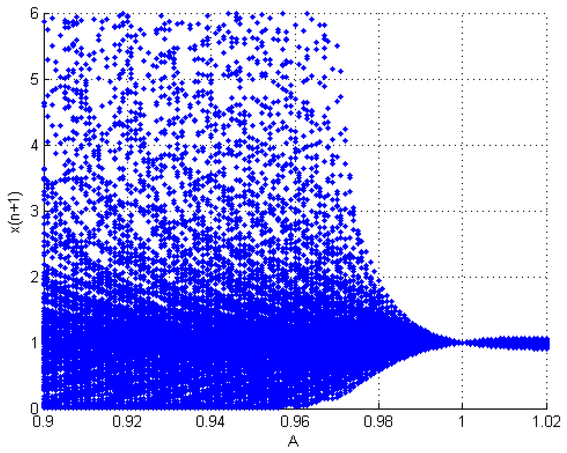
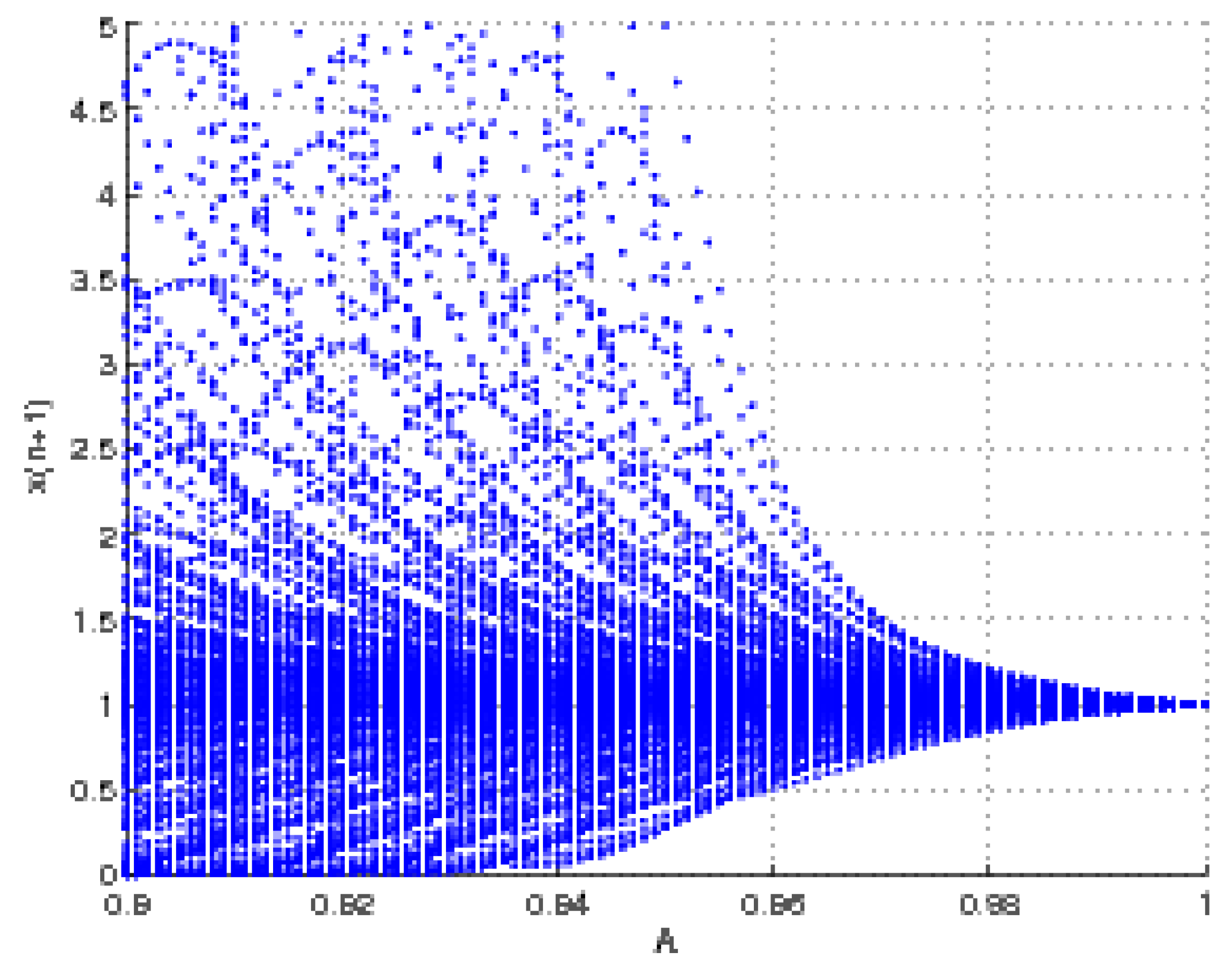
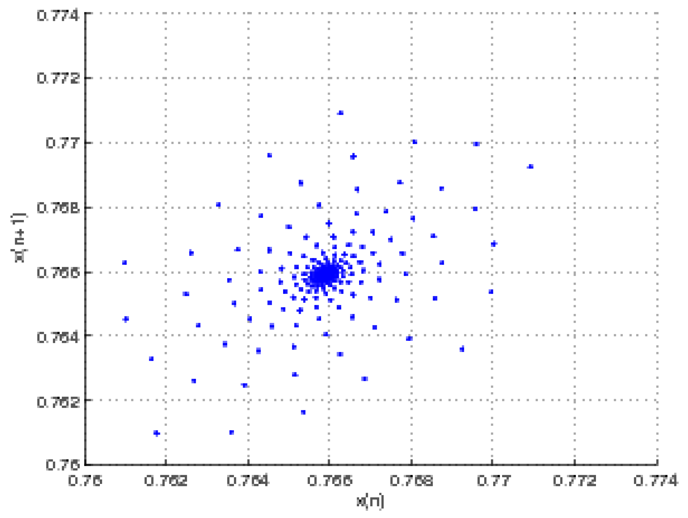
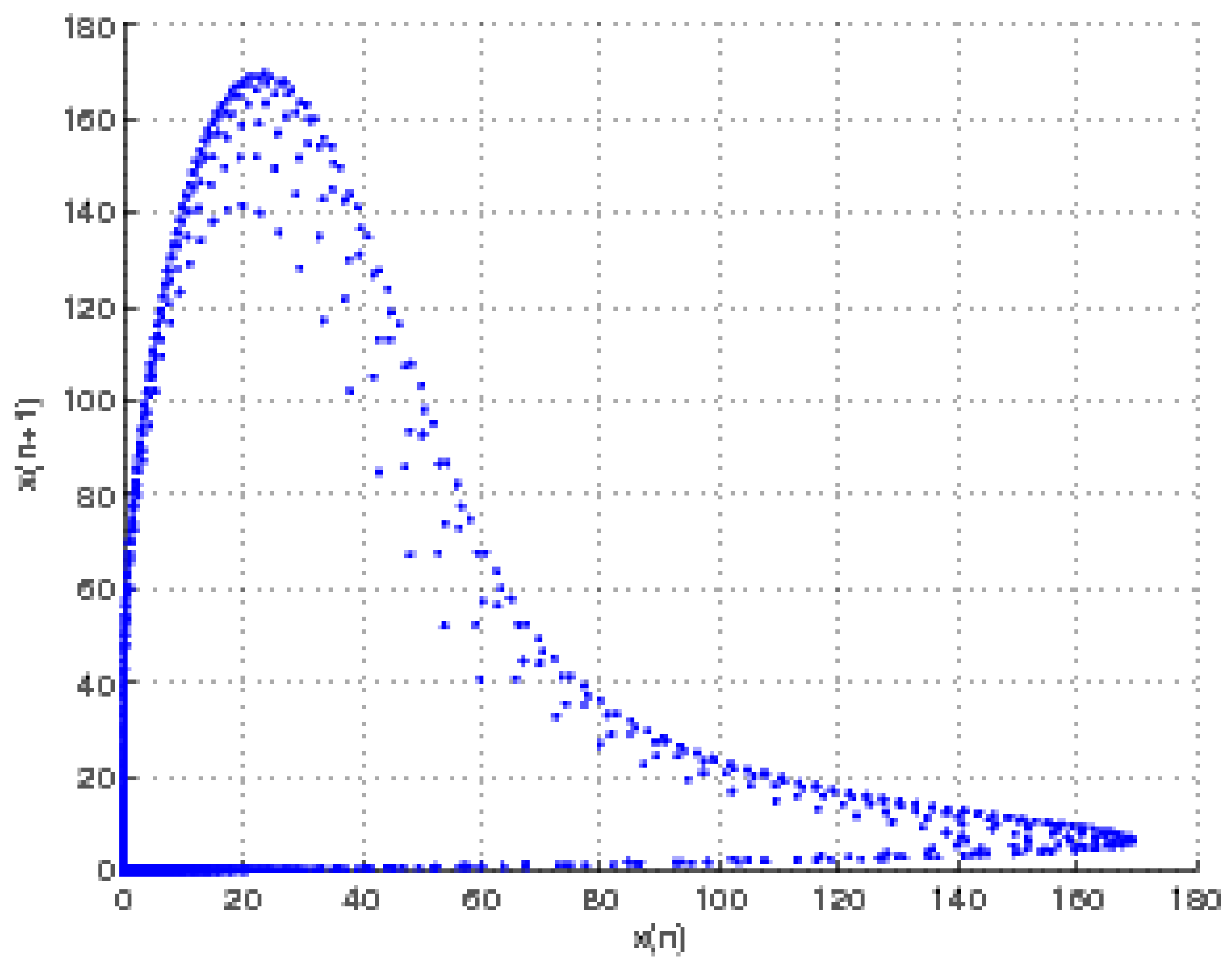
4. Numerical Simulation

In this section, we give numerical examples which support our result in previous section. For sake of simplicity, we take $c_n=x_n$, $\varsigma =B$, ${\varsigma }^{*}=B^{*}$ and $p=A$.

Example 1.

Let $B=1$ and $0.9<A<2$, then

$$x_{n+1}=\frac{x_n+x_{n-4}}{A+x_{n-1}}$$

(43)

with the initial conditions $x_0=x_{-1}=x_{-2}=x_{-3}=x_{-4}=1.$ (see Figure 2)

Example 2.

Let $B=0.9$ and $A=1.234$, then

$$x_{n+1}=\frac{0.9x_n+x_{n-4}}{\mathrm{1.234}+x_{n-1}}$$

(44)

with the initial condition $x_0=x_{-1}=x_{-3}=x_{-4}=x_{-5}=50$. (see Figure 3)

Example 3.

Let $B=0.889$ and $0.9<A<2$, then

$$x_{n+1}=\frac{0.889x_n+x_{n-4}}{1.1103+x_{n-1}}$$

(45)

with the initial condition $x_0=x_{-1}=x_{-3}=x_{-4}=x_{-5}=50$. (see Figure 2)

Example 4.

Let $B=1$ and $A=0.889$, then

$$x_{n+1}=\frac{x_n+x_{n-4}}{0.899+x_{n-1}}$$

(46)

with the initial conditions $x_0=x_{-1}=x_{-3}=x_{-4}=x_{-5}=1.7$. (see Figure 4)

5. Conclusions and Findings

We present some numerical simulations that support our theoretical results about the Neimark–Sacker bifurcation of model (11). We see a bifurcation diagram in Figure 1 in the (A, $x_{n+1}$) plane. In this figure, $B=1$, so the critical value of A at which Neimark–Sacker Bifurcation occurs is $A*$ = $0.9$, and the initial conditions are $c_{-4}=c_{-3}=c_{-2}=c_{-1}=c_0=1$. $A>0.9$ ensures the asymptotic stability of the positive fixed point. In Figure 3, we plot phase portrait by assigning the values $A=1.234$, $B=0.9$, $c_{-4}=c_{-3}=c_{-2}=c_{-1}=c_0$ = 50. Note that, for this value of A, the positive equilibrium point is asymptotically stable. Figure 4 and Figure 5 illustrate phase portraits by assigning values of A near the bifurcation point. In Figure 4, $A=1.1103$, $B=0.889$, $c_{-4}=c_{-3}=c_{-2}=c_{-1}=c_0$ = 50 while in Figure 5, $A=0.889$, $B=1$, $c_{-4}=c_{-3}=c_{-2}=c_{-1}=c_0$ = $1.7$. It is noticeable that we move away from the fixed point that the closed invariant curve disappears, which means the curve is subcritical (unstable). By virtue of Theorem 1, supported by Figure 1, the unique positive equilibrium $(1.1,1.1,1.1,1.1)$ in Figure 3 is unstable whereas in Figure 4, it is stable.

References

1. Camouzis, E.; Chatterjee, E.; Ladas, G. On the dynamics of xn+1 = ∂xn−2 + xn−3/A + xn−3. J. Math. Anal. Appl. 2007, 331, 230–239. [Google Scholar] [CrossRef] [Green Version]
2. Zhang, R.; Ding, X. The Neimark-Sacker bifurcation of xn+1 = ∂xn−2 + xn−3/A + xn−3. J. Differ. Equ. Appl. 2009, 15, 775–784. [Google Scholar]
3. Camouzis, E. Global analysis of solutions of xn+1 = ∂xn + xn−2/A + Bxn + Cxn−1. J. Math. Anal. Appl. 2005, 316, 616–627. [Google Scholar]
4. He, Z.; Qiu, J. Neimark-Sacker bifurcation of a third order rational difference equation. J. Differ. Equ. Appl. 2013, 19, 1513–1522. [Google Scholar] [CrossRef]
5. Camouzis, E.; Ladas, G. Dynamics of Third-order Rational Difference Equations with Open Problems and Conjectures. J. Differ. Equ. Appl. 2013, 19, 1513–1522. [Google Scholar]
6. Shareef, A.; Aloqeili, M. Neimark-Sacker bifurcation of a fourth order difference equation. Math. Meth. Appl. Sci. 2018, 19, 1–13. [Google Scholar] [CrossRef]
7. Kalabušic, S.; Kulenovic, M.R.S.; Mehuljic, M. Global dynamics and bifurcations of two quadratic fractional second-order difference equations. Comput. Anal. Appl. 2016, 21, 132–143. [Google Scholar]
8. Hrustic, S.J.; Kulenovic, M.R.S.; Nurkanovic, M. Global dynamics and bifurcations of certain second order rational difference equation with quadratic terms. Qual. Theory Dyn. 2016, 15, 283–307. [Google Scholar]
9. Kulenovic, M.R.S.; Moranjkic, S.; Nurkanovic, Z. Naimark-Sacker bifurcation of second order rational difference equation with quadratic terms. J. Nonlinear Sci. Appl. 2017, 10, 3377–3489. [Google Scholar] [CrossRef] [Green Version]
10. Valderde, J.C. Simplest normal forms of Hopf Neimark-Sacker Bifurcations. Int. J. Bifurc. Chaos 2003, 13, 1831–1839. [Google Scholar] [CrossRef]
11. Cushing, J.M. Difference equations as models of evolutionary population dynamics. J. Bio Dyn. 2019, 13, 103–127. [Google Scholar] [CrossRef] [Green Version]
12. Connor, M.K.; Pilav, E. The Neimark-Sacker bifurcation and global stability of perturbation of sigmoid beverton-holt difference equation. Dis. Dyn. Nat. Soc. 2021, 14, 2092709. [Google Scholar]
13. Kalabuši, S.; Kulenovi, M.P.S.; Mehulji, M. Global Period-Doubling Bifurcation of Quadratic Fractional Second Order Difference Equation. Dis. Dyn. Nat. Soc. 2014, 13, 10–53. [Google Scholar] [CrossRef]
14. Khaliq, A.; Alayachi, H.S.; Zubair, M.; Rohail, M.; Khan, A.Q. On stability analysis of a class of three-dimensional system of exponential difference equations. AIMS Math. 2023, 8, 5016–5035. [Google Scholar] [CrossRef]
15. Kuznetsov, Y.A.; Kuznetsov, I.A.; Kuznetsov, Y. Elements of Applied Bifurcation Theory, 3rd ed.; Springer Applied Mathematical Science: New York, NY, USA, 2013; p. 632. [Google Scholar]
16. Kocic, V.L.; Ladas, G. Global behaviour on non-linear difference equations of higher order with applications. Klu. Aca. Pub. 1993, 13, 10–53. [Google Scholar]
17. Khyat, T.; Kulenovic, M.; Pilav, E. The Naimark-Sacker bifurcation and asymptotic approximation of the invariant curve of a certain difference equation. J. Comp. Anal. Appl. 2017, 19, 15–22. [Google Scholar]
18. Hou, C.; Han, L.; Cheng, S. Complete Asymptotic and Bifurcation Analysis for a Difference Equation with Piece-wise Constant Control. Adv. Differ. Equ. 2010, 13, 542073. [Google Scholar]
19. Gari-Demirovi, M.; Moranjki, S. Neimark–Sacker Bifurcation and Approximation of the Invariant Curve of Certain Homogeneous Second-Order Fractional Difference Equation. Dis. Dyn. Nat. Soc. 2020, 12, 625–4013. [Google Scholar] [CrossRef]
20. Ibrahim, T.F. Bifurcation and periodically semi-cycles for fractional difference equation of fifth order. J. Nonlinear Sci. Appl. 2018, 11, 375–382. [Google Scholar] [CrossRef] [Green Version]
21. Stubna, M.D.; Gilmour, R.F. Analysis of a Non-linear Partial Difference Equation and Its Application to Cardiac Dynamics. J. Differ. Equ. Appl. 2010, 12, 1147–1169. [Google Scholar] [CrossRef]
Figure 1. Bifurcation diagram of Equation (9) in (A,x) plane.
Fractalfract 07 00113 g001
Figure 2. Neimark–Sacker bifurcation of the map x n + 1 = B x n + x n 4 A + x n 1 , where B = 1 and 0.9 < A < 2 , we can see that chaos shifted to stability at point A = 0.989 .
Fractalfract 07 00113 g002
Figure 3. Phase portraits of the map x n + 1 = 0.9 x n + x n 4 / 1.234 + x n 1 , for B = 0.9 .
Fractalfract 07 00113 g003
Figure 4. Phase portraits of the map x n + 1 = 0.8999 x n + x n 4 / 1.1103 + x n 1 , for B = B * .
Fractalfract 07 00113 g004
Figure 5. Phase portraits of the map x n + 1 = x n + x n 4 / 0.889 + x n 1 for B = B * .
Fractalfract 07 00113 g005
Disclaimer/Publisher’s Note: The statements, opinions and data contained in all publications are solely those of the individual author(s) and contributor(s) and not of MDPI and/or the editor(s). MDPI and/or the editor(s) disclaim responsibility for any injury to people or property resulting from any ideas, methods, instructions or products referred to in the content.