Necessary and Sufficient Conditions for Existence and Uniqueness of Solutions to Nabla Fractional Systems

Abstract

In this paper, we study the existence and uniqueness of solutions for nabla fractional systems. By using the properties of bijective functions, we obtain a necessary and sufficient condition ensuring the existence and uniqueness of solutions for a class of fractional discrete systems. Furthermore, we derive two sufficient conditions guaranteeing the existence of solutions by means of a nonlinear functional analysis method. In addition, the above conclusions are extended to high-dimensional delayed systems. Finally, two examples are given to illustrate the validity of our results.

1. Introduction

Recently, fractional differential systems have been widely applied in various fields, such as charge estimation, cybernetics, neural networks, viral transmission, and image encryption, see [1,2,3,4,5]. As the basis of these applications, the existence and uniqueness of solutions for fractional differential equations are crucial and have been explored in [6,7]. There are two kinds of problems about solutions; one is the boundary value problem (BVP), and the other is the initial value problem (IVP). BVP, which is mainly used in physics, studies finite time solutions in known boundary states [7,8]. IVP studies the solution of infinite time in the known initial state, which is the basis of equation stability and qualitative theory. Various forms of fractional differential IVP have been studied in the literature [9,10]. Goodrich et al. studied discrete fractional calculus systematically and obtained a general solution of IVP for a class of simple fractional difference systems in [11,12]. Boulares et al. in [13] explored the existence and uniqueness of solutions for nonlinear nabla fractional systems, and two fixed point theorems were used to prove the existence and uniqueness, respectively. He et al. in [14] presented a topological degree method to solve IVP of nonlinear fractional difference equations. For more studies on fractional nabla systems, see [15,16].

Consider the following nabla fractional nonlinear system:

$$\left\{\begin{array}{c}{}^C{\nabla }_d^{\gamma }x\left(m\right)=f\left(x\left(m\right)\right),m\in {\mathbb{N}}_{d+1},\hfill \\ x\left(d\right)=\varphi ,\hfill \end{array}\right.$$

(1)

where $0<\gamma <1,d\in \mathbb{R}$, ${}^C{\nabla }_d^{\gamma }$ is the nabla $\gamma$-th Caputo fractional operator, and f is a mapping from $\mathbb{D}\subseteq \mathbb{R}$ to $\mathbb{R}$, $\varphi \in \mathbb{D}$, ${\mathbb{N}}_d=\{d,d+1,d+2,\dots ,\}$. Most articles investigated the existence and uniqueness of solutions for fractional difference systems under the condition that $f\left(x\right)$ satisfies the global Lipschitz condition $\left|\right|f\left(x\right)-f\left(y\right)\left|\right|\le L\left|\right|x-y\left|\right|,\forall x,y\in \mathbb{R}$. However, a lot of functions, such as $f\left(x\right)=x^2$, $f\left(x\right)=e^x$ and various discontinuous functions, do not satisfy this condition. Then, it is natural to ask whether or not the Lipschitz condition is indispensable in the study of the existence and uniqueness of solutions to nabla fractional systems. If not necessary, what conditions should be established to ensure the existence and uniqueness of solutions; what methods can be adopted to obtain these conditions? Motivated by the above discussions, this paper investigates the existence and uniqueness of solutions to nabla fractional systems by using principle of finite induction. The main contributions and creative points of our paper are as follows:

Contribution 1: A new method using the principle of finite induction is proposed to explore the existence and uniqueness of solutions of nabla fractional systems for the first time.

Contribution 2: A sufficient and necessary condition on the existence and uniqueness for solutions of nabla fractional systems is given. Compared with [12,13], our condition required in this paper is less restrictive.

Contribution 3: Our conclusions can be extended to high-dimensional nonlinear systems with delays.

The structure of this paper is as follows. Some basic definitions and necessary lemmas are given in Section 2. In Section 3, we establish some sufficient and necessary conditions about the existence of unique solutions for one- and high-dimensional nabla fractional systems and give five useful corollaries. In Section 4, three examples are given to show that our conditions overcome some limitations in the existing literature.

2. Preliminaries

In this section, some necessary knowledge about discrete fractional calculus and nonlinear functional analysis are recapitulated.

Definition 1

([11]). (Generalized rising function) If $0<\gamma <1,$

$$m^{\overline{\gamma }}=\left\{\begin{array}{c}\frac{\mathrm{\Gamma }(m+\gamma )}{\mathrm{\Gamma }\left(m\right)},m\in \mathbb{R}\backslash {\mathbb{Z}}_{-},\hfill \\ 0,m\in {\mathbb{Z}}_{-},\hfill \end{array}\right.$$

where ${\mathbb{Z}}_{-}=\{\dots ,-2,-1,0\}$, and the Gamma function is defined by $\mathrm{\Gamma }\left(\kappa \right)={\int }_0^{+\infty }{e}^{-m}{m}^{\kappa -1}dm$.

Definition 2

([11]). (Nabla fractional sum) Assume $\phi :{\mathbb{N}}_{d+1}\mapsto \mathbb{R},\gamma >0$. Then, the γ-th sum is defined as

$${\nabla }_d^{-\gamma }\phi \left(m\right)=\frac{1}{\mathrm{\Gamma }\left(\gamma \right)}\sum _{\varpi =d+1}^m{\left(m-\rho \left(\varpi \right)\right)}^{\overline{\gamma -1}}\phi \left(\varpi \right),$$

where $\rho \left(\varpi \right)=\varpi -1$.

Definition 3

([11]). Assume $\phi :{\mathbb{N}}_d\mapsto \mathbb{R},\gamma >0$. Then, the nabla γ-th Caputo fractional operator is defined as

$${}^C{\nabla }_d^{\gamma }\phi \left(m\right)={\nabla }_d^{-(n-\gamma )}{\nabla }^n\phi \left(m\right),m\in {\mathbb{N}}_{d+1},$$

where $n=\lceil \gamma \rceil$, and $\lceil ·\rceil$ is the ceiling function.

Definition 4

([17]). $f:X\mapsto \mathbb{R}$ is called the invertible function, if there exists function $g:f\left(\mathbb{R}\right)\mapsto X$ satisfying $g\left(f\right(x\left)\right)=x,\forall x\in X$, and g is called the inverse function of f.

Lemma 1

([11]). Assume $\phi :{\mathbb{N}}_{d+1}\mapsto \mathbb{R}$, and γ, $\mu >0$. Then,

$${\nabla }_d^{-\gamma }{\nabla }_d^{-\mu }\phi \left(m\right)={\nabla }_d^{-\gamma -\mu }\phi \left(m\right),m\in {\mathbb{N}}_d.$$

Lemma 2

([18]). Let X be a Banach space and $\mathcal{F}:X\mapsto X$ be Lipschitz continuous with Lipschitz constant $k<1$. Then there exists a mapping $\mathcal{G}:X\mapsto X$ such that equation $x-\mathcal{F}\left(x\right)=y$ has a unique solution $x=y-\mathcal{G}\left(y\right)$.

Lemma 3

([17]). $\phi \left(x\right)$ is a monotone function defined from $(a,b)\subseteq \mathbb{R}$ to $\mathbb{E}\subseteq \mathbb{R}$ if and only if $\phi \left(x\right)$ is reversible and $\phi \left(\right(a,b\left)\right)=\mathbb{E}$.

3. Main Results

In this section, we first study a one-dimensional nabla fractional system and yield an important sufficient and necessary condition on the existence and uniqueness of solutions and give two useful corollaries. Furthermore, we extend the necessary and sufficient condition from a one-dimensional fractional difference system without time delay to a higher dimensional fractional difference system with time delay, and some useful corollaries are also derived.

Theorem 1.

For any initial value in $\mathbb{D}$, the solution of system (1) exists and is unique if and only if the function $h\left(x\right)=x-f\left(x\right)$ is reversible on $\mathbb{D}$ to $h\left(\mathbb{D}\right)$, $\mathbb{D}\subseteq \mathbb{R}$.

Proof. 

Sufficiency: Taking the fractional sum on both sides of (1) yields

$${\nabla }_d^{-\gamma }{}^C{\nabla }_d^{\gamma }x\left(m\right)={\nabla }_d^{-\gamma }f\left(x\left(m\right)\right),$$

(2)

then, on the basis of Definition 3, we derive

$${\nabla }_d^{-\gamma }{\nabla }_d^{-(1-\gamma )}\nabla x\left(m\right)={\nabla }_d^{-\gamma }f\left(x\left(m\right)\right).$$

(3)

Combining Lemma 1 with (3) yields

$${\nabla }_d^{-1}\nabla x\left(m\right)={\nabla }_d^{-\gamma }f\left(x\left(m\right)\right).$$

(4)

According to the properties of difference and Definition 2, one has

$$x\left(m\right)-x\left(d\right)=\frac{1}{\mathrm{\Gamma }\left(\gamma \right)}\sum _{\varpi =d+1}^m{\left(m-\rho \left(\varpi \right)\right)}^{\overline{\gamma -1}}f\left(x\left(\varpi \right)\right),$$

(5)

it follows from (5) that

$$x\left(m\right)=x\left(d\right)+\frac{1}{\mathrm{\Gamma }\left(\gamma \right)}\sum _{\varpi =d+1}^{m-1}{\left(m-\rho \left(\varpi \right)\right)}^{\overline{\gamma -1}}f\left(x\left(\varpi \right)\right)+\frac{1}{\mathrm{\Gamma }\left(\gamma \right)}{\left(m-\rho \left(m\right)\right)}^{\overline{\gamma -1}}f\left(x\left(m\right)\right).$$

(6)

Then, according to Definition 1, one can obtain

$$x\left(m\right)-f\left(x\left(m\right)\right)=x\left(d\right)+\frac{1}{\mathrm{\Gamma }\left(\gamma \right)}\sum _{\varpi =d+1}^{m-1}{\left(m-\rho \left(\varpi \right)\right)}^{\overline{\gamma -1}}f\left(x\left(\varpi \right)\right).$$

(7)

Because $h\left(x\right)=x-f\left(x\right)$ is reversible, then there exists a function $g\left(x\right):\mathbb{R}\mapsto \mathbb{D}$, $g\left(x-f\left(x\right)\right)=x$. From (7), we can obtain the following recursive formula:

$$\begin{array}{cc}\hfill & x\left(d\right)=\varphi ,\hfill \\ \hfill & x(d+1)=g\left(x\left(d\right)\right),\hfill \\ \hfill & x(d+2)=g\left[x\left(d\right)+\frac{1}{\mathrm{\Gamma }\left(\gamma \right)}{2}^{\overline{\gamma -1}}f\left(x(d+1)\right)\right],\hfill \\ \hfill & ⋮\hfill \\ \hfill & x(d+n)=g\left[x\left(d\right)+\frac{1}{\mathrm{\Gamma }\left(\gamma \right)}\sum _{\varpi =d+1}^{d+n-1}{\left(d+n-\rho \left(\varpi \right)\right)}^{\overline{\gamma -1}}f\left(x\left(\varpi \right)\right)\right],\hfill \end{array}$$

(8)

by using the principle of finite induction, the unique solution $x\left(m\right)$ of initial value $x\left(d\right)=\varphi$ can be found.

Necessity: We show that function $h\left(x\right)$ must be a one-to-one mapping by using reduction to absurdity.

If $h\left(x\right)$ is not injective, then there must exist $x_1$, $x_2\in \mathbb{D}$, such that

$$h\left(x_1\right)=h\left(x_2\right)=\varrho ,$$

(9)

it follows from (7) that

$$\begin{array}{c}\hfill x(d+1)-f\left(x\right(d+1\left)\right)=h\left(x\right(d+1\left)\right)=x\left(d\right).\end{array}$$

(10)

The solution is unique for any initial value, but $x(d+1)$ could be equal to $x_1$ or $x_2$ when the initial value $x\left(d\right)=\varrho$, which is contradicted with the uniqueness.

If $h\left(x\right)$ is not surjective, then there must exist $\varrho$ such that

$$h\left(x\right)\ne \varrho ,\forall x\in \mathbb{D}.$$

(11)

The solution exists for any initial value, but Equation (10) does not hold when the initial value $x\left(d\right)=\varrho$ for any $x(d+1)\in \mathbb{D}$, which is contradicted. □

Remark 1.

The general solution of IVP ${}^C{\nabla }_d^{\gamma }x\left(m\right)=f\left(m\right)$ is given in reference [11]. If $f\left(x\right)$ is changed into $f\left(x\right(m\left)\right)$, then the nonlinear Equation (7) may have no solution. We note that the existence and uniqueness of the solution to the nonlinear Equation (7) are equivalent to that of the system (1).

Although the above theorem gives a sufficient and necessary condition, it is difficult to judge whether the function h is invertible or not. The inverse of the function is also difficult to be expressed by elementary function. Using Lemmas 2 and 3, the following two useful corollaries can be acquired directly.

Corollary 1.

For system (1), if the function $f\left(x\right)$ is a contraction map, then the solutions of system (1) are existing and unique.

Corollary 2.

The solution of system (1) with initial value $x\left(d\right)\in \mathbb{D}=(a,b)$ exists if and only if $h\left(x\right)=x-f\left(x\right)$ is monotone on $(a,b)$ and $h\left(\right(a,b\left)\right)=\mathbb{R}$.

Remark 2.

Two algorithms that can make the numerical simulation error arbitrarily small are naturally derived from the above two corollaries. The inverse function of the monotone function in Corollary 2 can be approximated by dichotomy. The inverse function of the function in Corollary 1 can be approximated arbitrarily by a fixed point iterative method.

Theorem 2.

If system (1) has a solution $x\left(t\right)$ satisfying ${\displaystyle \underset{m\to +\infty }{lim}x\left(m\right)=x^{*}}$ and function $f\left(x\right)$ satisfies ${\displaystyle \underset{m\to +\infty }{lim}f\left(x\left(m\right)\right)=B}$, then $B=0$.

Proof. 

Reduction to absurdity is employed in this theorem. If $B>0$, then there exists $N_1$ such that $f\left(x\left(m_1\right)\right)>\frac{1}{2}B,m_1>N_1$. On the other hand, taking the limit of t for both sides of Equation (5), we obtain

$${\displaystyle \underset{m\to +\infty }{lim}\sum _{\varpi =d+1}^m{\left(m-\rho \left(\varpi \right)\right)}^{\overline{\gamma -1}}f\left(x\left(\varpi \right)\right)=\mathrm{\Gamma }\left(\gamma \right)(x^{*}-x\left(d\right)),}$$

(12)

which means ${\displaystyle \sum _{\varpi =d+1}^m{\left(m-\rho \left(\varpi \right)\right)}^{\overline{\gamma -1}}f\left(x\left(\varpi \right)\right)}$ must be convergent. Because of

$$\begin{array}{cc}\hfill & {\displaystyle \underset{m\to +\infty }{lim}\sum _{\varpi =d+1}^{N_1}{\left(m-\rho \left(\varpi \right)\right)}^{\overline{\gamma -1}}f\left(x\left(\varpi \right)\right)}\hfill \\ \hfill & {\displaystyle \le \underset{m\to +\infty }{lim}\underset{\varpi \le N_1}{max}\left\{f\left(x\left(\varpi \right)\right)\right\}\sum _{\varpi =d+1}^{N_1}{\left(m-\rho \left(\varpi \right)\right)}^{\overline{\gamma -1}}}\hfill \\ \hfill & {\displaystyle \le \underset{m\to +\infty }{lim}(N_1-d){(m-N_1)}^{\overline{\gamma -1}}\underset{\varpi \le N_1}{max}\left\{f\left(x\left(\varpi \right)\right)\right\}}\hfill \\ \hfill & =0,\hfill \end{array}$$

(13)

we obtain

$$\begin{array}{cc}\hfill & {\displaystyle \underset{m\to +\infty }{lim}\sum _{\varpi =d+1}^m{\left(m-\rho \left(\varpi \right)\right)}^{\overline{\gamma -1}}f\left(x\left(\varpi \right)\right)}\hfill \\ \hfill & {\displaystyle =\underset{m\to +\infty }{lim}\sum _{\varpi =d+1}^{N_1}{\left(m-\rho \left(\varpi \right)\right)}^{\overline{\gamma -1}}f\left(x\left(\varpi \right)\right)+\underset{m\to +\infty }{lim}\sum _{\varpi =N_1+1}^m{\left(m-\rho \left(\varpi \right)\right)}^{\overline{\gamma -1}}f\left(x\left(\varpi \right)\right)}\hfill \\ \hfill & {\displaystyle \ge \underset{m\to +\infty }{lim}\frac{1}{2}\sum _{\varpi =N_1+1}^m{\left(m-\rho \left(\varpi \right)\right)}^{\overline{\gamma -1}}f\left(x^{*}\right)}\hfill \\ \hfill & {\displaystyle =\underset{m\to +\infty }{lim}\frac{1}{2\gamma }\left({\left(m-N_1\right)}^{\overline{\gamma }}-1\right)f\left(x^{*}\right)}\hfill \\ \hfill & =+\infty ,\hfill \end{array}$$

(14)

which contradicts Equation (12), so $B>0$ is false. Similarly, we can show $B<0$ is false. □

Then, we come to the conclusion $B=0$.

Corollary 3.

If system (1) has a unique solution to any initial value $x\left(d\right)\in (a,b)$, and there exists $x\left(m\right)$ satisfying ${\displaystyle \underset{m\to +\infty }{lim}x\left(m\right)=x^{*}}$ and $f\in C\left(\right(a,b),\mathbb{R})$, then ${\displaystyle \underset{m\to +\infty }{lim}f\left(x\left(m\right)\right)=0}$.

Proof. 

Using Theorem 2, we simply prove that $f\left(x\right(m\left)\right)$ has a limit. We categorize the following two cases.

• Case 1: $x^{*}\in (a,b)$. According to $f\in C\left(\right(a,b),\mathbb{R})$ and the Heine theorem, we have ${\displaystyle \underset{m\to +\infty }{lim}f\left(x\left(m\right)\right)=f\left(x^{*}\right)}$.
• Case 2: $x^{*}\notin (a,b)$. Since ${\displaystyle \underset{m\to +\infty }{lim}x\left(m\right)=x^{*}}$ and $x\left(m\right)\in (a,b),\forall m\in {\mathbb{N}}_{d+1}$, we obtain ${\displaystyle \underset{m\to +\infty }{lim}x\left(m\right)=b=x^{*}}$ or ${\displaystyle \underset{m\to +\infty }{lim}x\left(m\right)=a=x^{*}}$. Without losing generality, let us say that $b=x^{*}$.

Using the necessity of Corollary 2, function $h\left(x\right)=x-f\left(x\right)$ is monotone. If $h\left(x\right)$ is monotonically increasing, we first prove $h\left(x\right)$ is bounded. Assuming ${\displaystyle \underset{x\to b}{lim}h\left(x\right)=+\infty }$, then we can obtain

$${\displaystyle \underset{m\to +\infty }{lim}f\left(x\left(m\right)\right)=\underset{x\to b}{lim}f\left(x\right)=\underset{x\to b}{lim}(b-h\left(x\right))=-\infty ,}$$

(15)

using the above equation, we have

$${\displaystyle \underset{m\to +\infty }{lim}\left(x\left(d\right)+\frac{1}{\mathrm{\Gamma }\left(\gamma \right)}\sum _{\varpi =d+1}^{m-1}{\left(m-\rho \left(\varpi \right)\right)}^{\overline{\gamma -1}}f\left(x\left(\varpi \right)\right)\right)=-\infty ,}$$

(16)

which contradicts Equation (7), so $h\left(x\right)$ is bounded, and because h is a monotone function, there exists $\mathrm{\Lambda }$ such that ${\displaystyle \underset{x\to b}{lim}h\left(x\right)=\mathrm{\Lambda }}$ and ${\displaystyle \underset{m\to +\infty }{lim}f\left(x\left(m\right)\right)=\mathrm{\Lambda }-x^{*}}$. Similarly, we can obtain that $f\left(x\right(m\left)\right)$ has a limit when $h\left(x\right)$ is decreasing monotonically. □

Remark 3.

Corollary 3 shows that if the solution of the system (1) is asymptotically stable and the function f is defined on the interval $\mathbb{D}\subseteq \mathbb{R}$, then $f\left(x\right(m\left)\right)$ must approach 0, which is similar to integer-order continuous system and is helpful for us to study the Lyapunov method of the fractional-order difference system.

The above discussion mainly focuses on a one-dimensional system without delay, but in practical applications, high-dimensional systems with delays are more widely used. Let us discuss more general high-dimensional systems with delays, which are described as follows:

$$\left\{\begin{array}{c}{}^C{\nabla }_d^{\gamma }\mathcal{X}\left(m\right)=\mathcal{A}\mathcal{X}\left(m\right)+\mathcal{B}\mathcal{X}(m-\tau )+f\left(\mathcal{X}\left(m\right)\right)+g\left(\mathcal{X}(m-\tau )\right),m\in {\mathbb{N}}_{d+1},\hfill \\ \mathcal{X}\left(\zeta \right)=\mathrm{\Phi }\left(\zeta \right),\zeta \in \{d-\tau ,d-\tau +2,\dots ,d\},\hfill \end{array}\right.$$

(17)

where $0<\gamma <1$, $\mathrm{\Phi }\left(\zeta \right)\in \mathbb{D},\zeta \in \{d-\tau +1,d-\tau +2,\dots ,d\}$; $\mathcal{A}$, $\mathcal{B}$ are $n\times n$ constant matrices; $\tau \in {\mathbb{Z}}^{+}$ denotes the time delay, $f\left(x\right)$, $g\left(x\right)$ are nonlinear functions defined from $\mathbb{D}$ to ${\mathbb{R}}^n$, and $\mathbb{D}\subseteq {\mathbb{R}}^n$.

Theorem 3.

For any initial value function $\mathrm{\Phi }:\{d-\tau +1,d-\tau +2,\dots ,d\}\mapsto \mathbb{D}$, the solution of the system (17) exists and is unique if and only if the function $\mathcal{H}\left(\mathcal{X}\right)=\mathcal{X}-\mathcal{AX}-f\left(\mathcal{X}\right)$ is reversible.

Proof. 

Sufficiency: Taking the fractional sum on both sides of (17) yields

$${\nabla }_d^{-\gamma }{}^C{\nabla }_d^{\gamma }\mathcal{X}\left(m\right)={\nabla }_d^{-\gamma }\left[\mathcal{AX}\left(m\right)+\mathcal{BX}(m-\tau )+f\left(\mathcal{X}\left(m\right)\right)+g\left(\mathcal{X}(m-\tau )\right)\right],$$

(18)

on the basis of Definition 3 and Lemma 1, one derives

$$\begin{array}{ccc}{\displaystyle {\nabla }_d^{-1}{\nabla }^1\mathcal{X}\left(m\right)}& =& {\displaystyle \frac{1}{\mathrm{\Gamma }\left(\gamma \right)}\sum _{\varpi =d+1}^m{(m-\rho \left(\varpi \right))}^{\overline{\gamma -1}}[\mathcal{AX}\left(\varpi \right)+\mathcal{BX}(\varpi -\tau )}\hfill \\ & & {\displaystyle +f\left(\mathcal{X}\left(\varpi \right)\right)+g\left(\mathcal{X}(\varpi -\tau )\right)],}\hfill \end{array}$$

(19)

then according to the properties of the nabla difference operator, we obtain

$$\begin{array}{cc}\hfill \mathcal{X}\left(m\right)-\mathcal{X}\left(d\right)=& \frac{1}{\mathrm{\Gamma }\left(\gamma \right)}\sum _{\varpi =d+1}^m{\left(m-\rho \left(\varpi \right)\right)}^{\overline{\gamma -1}}\left[\mathcal{AX}\left(\varpi \right)+f\left(\mathcal{X}\left(\varpi \right)\right)\right]\hfill \\ \hfill & +\frac{1}{\mathrm{\Gamma }\left(\gamma \right)}\sum _{\varpi =d+1}^m{\left(m-\rho \left(\varpi \right)\right)}^{\overline{\gamma -1}}\left[\mathcal{BX}(\varpi -\tau )+g\left(\mathcal{X}(\varpi -\tau )\right)\right],\hfill \end{array}$$

(20)

it follows from (20) that

$$\begin{array}{cc}\hfill \mathcal{X}\left(m\right)=& \mathcal{X}\left(d\right)+\frac{1}{\mathrm{\Gamma }\left(\gamma \right)}\sum _{\varpi =d+1}^{m-1}{\left(m-\rho \left(\varpi \right)\right)}^{\overline{\gamma -1}}\left[\mathcal{AX}\left(\varpi \right)+f\left(\mathcal{X}\left(\varpi \right)\right)\right]\hfill \\ \hfill & +\frac{1}{\mathrm{\Gamma }\left(\gamma \right)}\sum _{\varpi =d+1}^m{\left(m-\rho \left(\varpi \right)\right)}^{\overline{\gamma -1}}[\mathcal{BX}(\varpi -\tau )\hfill \\ \hfill & +g\left(\mathcal{X}(\varpi -\tau )\right)]+\mathcal{AX}\left(m\right)+f\left(\mathcal{X}\left(m\right)\right).\hfill \end{array}$$

(21)

Based on Definition 1, we obtain

$$\begin{array}{cc}\hfill & {\displaystyle \mathcal{X}\left(m\right)-\mathcal{AX}\left(m\right)-f\left(\mathcal{X}\left(m\right)\right)}\hfill \\ =\hfill & {\displaystyle \mathcal{X}\left(d\right)+\frac{1}{\mathrm{\Gamma }\left(\gamma \right)}\sum _{\varpi =d+1}^{m-1}{\left(m-\rho \left(\varpi \right)\right)}^{\overline{\gamma -1}}\left[\mathcal{AX}\left(\varpi \right)+f\left(\mathcal{X}\left(\varpi \right)\right)\right]}\hfill \\ \hfill & {\displaystyle +\frac{1}{\mathrm{\Gamma }\left(\gamma \right)}\sum _{\varpi =d+1}^m{\left(m-\rho \left(\varpi \right)\right)}^{\overline{\gamma -1}}\left[\mathcal{BX}(\varpi -\tau )+g\left(\mathcal{X}(\varpi -\tau )\right)\right],}\hfill \end{array}$$

(22)

and since $\mathcal{H}\left(\mathcal{X}\right)=\mathcal{X}-\mathcal{AX}-f\left(\mathcal{X}\right)$ is reversible, then there exists a function $\mathcal{G}\left(\mathcal{X}\right)$ that satisfies $\mathcal{G}(\mathcal{X}-\mathcal{AX}-f(\mathcal{X}\left)\right)=\mathcal{X}$. According to Equation (22), we can obtain the recursive formula as follows:

$$\begin{array}{cc}\hfill & \mathcal{X}\left(d\right)=\mathrm{\Phi }\left(d\right),\hfill \\ \hfill & \mathcal{X}(d+1)=\mathcal{G}\left[\mathcal{X}\left(d\right)+\mathcal{B}\mathrm{\Phi }(d+1-\tau )+g\left(\mathrm{\Phi }(d+1-\tau )\right)\right],\hfill \\ \hfill & \mathcal{X}(d+2)=\mathcal{G}[\mathcal{X}\left(d\right)+\mathcal{B}\mathrm{\Phi }(d+2-\tau )+g\left(\mathrm{\Phi }(d+2-\tau )\right)\hfill \\ \hfill & +\frac{1}{\mathrm{\Gamma }\left(\gamma \right)}{2}^{\overline{\gamma -1}}\left(\mathcal{AX}(d+1)+f\left(\mathcal{X}(d+1)\right)\right)\hfill \\ \hfill & +\mathcal{B}\mathrm{\Phi }(d+1-\tau )+g\left(\mathrm{\Phi }(d+1-\tau )\right)],\hfill \\ \hfill & ⋮\hfill \\ \hfill & \mathcal{X}(d+n)=\mathcal{G}[\mathcal{X}\left(d\right)+\frac{1}{\mathrm{\Gamma }\left(\gamma \right)}\sum _{\varpi =d+1}^{d+n-1}{(d+n-\rho \left(\varpi \right))}^{\overline{\gamma -1}}\left(\mathcal{AX}\left(\varpi \right)+f\left(\mathcal{X}\left(\varpi \right)\right)\right)\hfill \\ \hfill & +\frac{1}{\mathrm{\Gamma }\left(\gamma \right)}\sum _{\varpi =d+1}^{d+n}{(d+n-\rho \left(\varpi \right))}^{\overline{\gamma -1}}\left(\mathcal{BX}(\varpi -\tau )+g\left(\mathcal{X}(\varpi -\tau )\right)\right)],\hfill \end{array}$$

(23)

$\mathcal{X}\left(m\right)$ can be uniquely obtained from the above recurrence equation by using the principle of finite induction.

Necessity: We prove that function $\mathcal{H}\left(\mathcal{X}\right)$ must be a one-to-one mapping by employing reduction to absurdity.

If $\mathcal{H}\left(\mathcal{X}\right)$ is not injective, then there must exist ${\mathcal{X}}_1$, ${\mathcal{X}}_2$ such that

$$\mathcal{H}\left({\mathcal{X}}_1\right)=\mathcal{H}\left({\mathcal{X}}_2\right)=y,$$

(24)

it follows from Equation (22) that

$$\begin{array}{cc}& \mathcal{X}(d+1)-\mathcal{AX}(d+1)-f\left(\mathcal{X}(d+1)\right)\hfill \\ \hfill =& \mathcal{H}\left(\mathcal{X}(d+1)\right)=\mathcal{X}\left(d\right)+\mathcal{B}\left(\mathrm{\Phi }(d+1-\tau )\right)+g\left(\mathrm{\Phi }(d+1-\tau )\right).\hfill \end{array}$$

(25)

System (17) has a unique solution, but if the initial value function $\mathrm{\Phi }$ satisfies $\mathrm{\Phi }\left(\zeta \right)=0$, $\zeta <d$, $\mathrm{\Phi }\left(d\right)=y-g\left(0\right)$, $\mathcal{X}(d+1)$ could be equal to ${\mathcal{X}}_1$ or ${\mathcal{X}}_2$, which contradicts the uniqueness.

If $\mathcal{H}\left(\mathcal{X}\right)$ is not surjective, then there must exist y such that

$$\mathcal{H}\left(\mathcal{X}\right)\ne y,\forall \mathcal{X}\in {\mathbb{R}}^n,$$

(26)

then if the initial value function $\mathrm{\Phi }$ satisfies $\mathrm{\Phi }\left(\zeta \right)=0$, $\zeta <d$ and $\mathrm{\Phi }\left(d\right)=y-g\left(0\right)$, from Equation (25), we obtain the following equation

$$\mathcal{H}\left(\mathcal{X}(d+1)\right)=\mathrm{\Phi }\left(d\right)+\mathcal{B}\left(\mathrm{\Phi }(d+1-\tau )\right)+g\left(\mathrm{\Phi }(d+1-\tau )\right)=y-g\left(0\right)+g\left(0\right)=y,$$

(27)

which contradicts Equation (26). □

Using Theorem 3, we have the following corollaries.

Corollary 4.

For any initial value function $\mathrm{\Phi }:\{d-\tau +1,d-\tau +2,\dots ,d\}\mapsto \mathbb{D}$, the solution of the system

$$\left\{\begin{array}{c}{}^C{\nabla }_d^{\gamma }\mathcal{X}\left(m\right)=\mathcal{AX}\left(m\right)+\mathcal{BX}(m-\tau )+g\left(\mathcal{X}(m-\tau )\right),m\in {\mathbb{N}}_{d+1},0<\gamma <1,\hfill \\ \mathcal{X}\left(\zeta \right)=\mathrm{\Phi }\left(\zeta \right),\zeta \in \{d-\tau +1,d-\tau +2,\dots ,d\},\hfill \end{array}\right.$$

(28)

exists and is unique if and only if ${\lambda }_i\left(\mathcal{A}\right)\ne 1$, where ${\lambda }_i\left(\mathcal{A}\right)$ is the i-th eigenvalue of $\mathcal{A}$.

Corollary 5.

The solution of the system

$$\left\{\begin{array}{c}{}^C{\nabla }_d^{\gamma }\mathcal{X}\left(m\right)=\mathcal{BX}(m-\tau )+g\left(x(m-\tau )\right),m\in {\mathbb{N}}_{d+1},0<\gamma <1,\hfill \\ \mathcal{X}\left(\zeta \right)=\mathrm{\Phi }\left(\zeta \right),\zeta \in \{d-\tau ,d-\tau +2,\dots ,d\},\hfill \end{array}\right.$$

(29)

exists and is unique.

Remark 4.

Corollaries 3 and 4 show that time delays are independent of the existence and uniqueness for solutions of discrete systems, which are different from continuous systems. In practical applications, time delays are almost inevitable, which guarantee the existence and uniqueness of solutions for most more complex real models.

By using Lemma 2, we can draw the following corollary immediately.

Corollary 6.

For system (17), if function $\mathcal{H}\left(\mathcal{X}\right)=\mathcal{AX}+f\left(\mathcal{X}\right)$ satisfies $\left|\right|\mathcal{H}\left(x\right)-\mathcal{H}\left(y\right)\left|\right|<k\left|\right|x-y\left|\right|,k<1$, then the solutions of system (17) are existing and unique.

Remark 5.

Compared with Theorem 3.2 in [14], novelties of this paper are as follows: on the one hand, the effect of time delay is considered in our system (17). On the other hand, a new method is proposed to study the existence of solutions. In addition, compared with Theorem 3.2 in [10], we do not need to put any constraints on the delay term.

In proving the necessity of Theorem 2, we find that uniqueness is mainly determined by injectivity of function $\mathcal{H}\left(\mathcal{X}\right)$. Can we use the surjective property of the function to obtain the existence of the solution directly? We give the following theorem.

Theorem 4.

The solutions of system (17) exist if $\mathcal{H}\left(\mathbb{D}\right)={\mathbb{R}}^n$.

Proof. 

Since the the range of $\mathcal{H}\left(\mathcal{X}\right)$ is ${\mathbb{R}}^n$, we can find a subset $\mathbb{S}$ of $\mathbb{D}$ such that mapping H constrained on the set $\mathbb{S}$ is a one-to-one mapping and is denoted as ${\mathcal{H}|}_{\mathbb{S}}$. According to Equation (22) and ${\mathcal{H}|}_{\mathbb{S}}$, we obtain

$$\begin{array}{ccc}& \hfill & {\left(\mathcal{H}{|}_{\mathbb{S}}\right)}^{-1}\left[\mathcal{X}\left(m\right)-\mathcal{AX}\left(m\right)-f\left(\mathcal{X}\left(m\right)\right)\right]\hfill \\ & =\hfill & {\displaystyle {\left(\mathcal{H}{|}_{\mathbb{S}}\right)}^{-1}(\mathcal{X}\left(d\right)+\frac{1}{\mathrm{\Gamma }\left(\gamma \right)}\sum _{\varpi =d+1}^{m-1}{\left(m-\rho \left(\varpi \right)\right)}^{\overline{\gamma -1}}\left[\mathcal{AX}\left(\varpi \right)+f\left(\mathcal{X}\left(\varpi \right)\right)\right]}\hfill \\ & \hfill & {\displaystyle +\frac{1}{\mathrm{\Gamma }\left(\gamma \right)}\sum _{\varpi =d+1}^t{\left(m-\rho \left(\varpi \right)\right)}^{\overline{\gamma -1}}\left[\mathcal{BX}(\varpi -\tau )+g\left(\mathcal{X}(\varpi -\tau )\right)\right]).}\hfill \end{array}$$

(30)

Therefore we can obtain a solution that satisfies the following recursive formula:

$$\begin{array}{cc}\hfill & \mathcal{X}\left(d\right)=\mathrm{\Phi }\left(d\right),\hfill \\ \hfill & \mathcal{X}(d+1)={\left(\mathcal{H}{|}_{\mathbb{S}}\right)}^{-1}\left[\mathcal{X}\left(d\right)+\mathcal{B}\mathrm{\Phi }(d+1-\tau )+g\left(\mathrm{\Phi }(d+1-\tau )\right)\right],\hfill \\ \hfill & +\mathcal{B}\mathrm{\Phi }(d+1-\tau )+g\left(\mathrm{\Phi }(d+1-\tau )\right)],\hfill \\ \hfill & ⋮\hfill \\ \hfill & \mathcal{X}(d+n)={\left(\mathcal{H}{|}_{\mathbb{S}}\right)}^{-1}[\mathcal{X}\left(d\right)+\frac{1}{\mathrm{\Gamma }\left(\gamma \right)}\sum _{\varpi =d+1}^{d+n-1}{(d+n-\rho \left(\varpi \right))}^{\overline{\gamma -1}}\left(\mathcal{AX}\left(\varpi \right)+f\left(\mathcal{X}\left(\varpi \right)\right)\right)\hfill \\ \hfill & +\frac{1}{\mathrm{\Gamma }\left(\gamma \right)}\sum _{\varpi =d+1}^{d+n}{(d+n-\rho \left(\varpi \right))}^{\overline{\gamma -1}}\left(\mathcal{BX}(\varpi -\tau )+g\left(\mathcal{X}(\varpi -\tau )\right)\right)].\hfill \end{array}$$

(31)

□

4. Numerical Simulations

In this section, we use three examples to show the validity of our results.

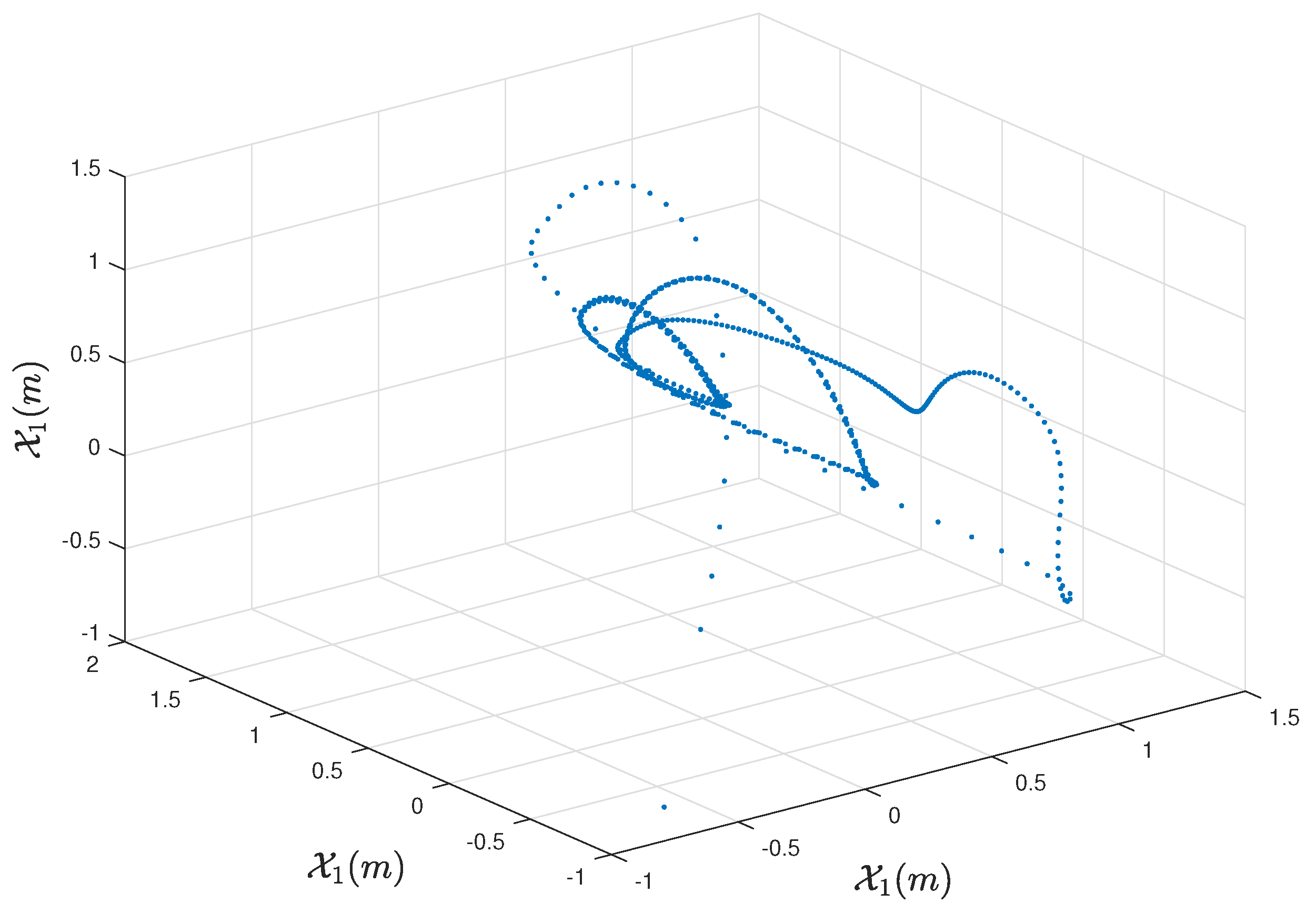
Example 1.

Consider the following system

$$\left\{\begin{array}{c}{}^C{\nabla }_0^{0.9}\phi \left(m\right)=\phi \left(m\right)+ln\left(\phi \left(m\right)\right),\hfill \\ \phi \left(0\right)=1.6.\hfill \end{array}\right.$$

(32)

In (32), $f\left(\phi \right)=\phi +ln\left(\phi \right)$ does not satisfy the Lipschitz condition because $sup\frac{f\left(\phi \right)-f\left(\varphi \right)}{\phi -\varphi }=+\infty$. However, from $g\left(\phi \right)=e^{-\phi }$ and $g(\phi -f(\phi \left)\right)=\phi$, we can derive the following recurrence:

$$\begin{array}{cc}\hfill & \phi \left(0\right)=1,\hfill \\ \hfill & \phi \left(1\right)=e^{-\phi \left(0\right)},\hfill \\ \hfill & \phi \left(2\right)=e^{-(\phi \left(0\right)+\frac{1}{\mathrm{\Gamma }\left(0.9\right)}{2}^{\overline{-0.1}}(\phi \left(1\right)+ln\left(\phi \left(1\right)\right))},\hfill \\ \hfill & ⋮\hfill \\ \hfill & \phi (d+n)=e^{-(\phi \left(0\right)+\frac{1}{\mathrm{\Gamma }\left(0.9\right)}{\sum }_{\varpi =1}^{n-1}{(t-\rho \left(\varpi \right))}^{\overline{-0.1}}(\phi \left(\varpi \right)+ln\left(\phi \left(\varpi \right)\right))},\hfill \end{array}$$

(33)

so this example shows that even if $f\left(\phi \right)$ does not satisfy the Lipschitz condition, the system still has a unique solution as long as $\phi -f\left(\phi \right)$ is invertible. It can even be seen from Figure 1 that system (32) is asymptotically stable to ${\phi }^{*}$, where ${\phi }^{*}$ satisfies ${\phi }^{*}+ln\left({\phi }^{*}\right)=0$.

Example 2.

Consider the system

$$\left\{\begin{array}{c}{}^C{\nabla }_0^{0.95}\mathcal{X}\left(m\right)=\mathcal{A}\mathcal{X}\left(m\right)+\mathcal{B}f\left(\mathcal{X}\left(m\right)\right)+\mathcal{C}g\left(\mathcal{X}(m-3)\right),\hfill \\ \mathcal{X}\left(\zeta \right)=\left(\genfrac{}{}{0pt}{}{1.6}{-0.7}\right),\zeta \in \{-3,-2,-1,0\},\hfill \end{array}\right.$$

(34)

where $\mathcal{A}=\left(\begin{array}{cc}-0.1& 0\\ 0& -0.1\end{array}\right)$, $\mathcal{B}=\left(\begin{array}{cc}0& 0.3\\ -0.3& 0\end{array}\right)$, $\mathcal{C}=\left(\begin{array}{cc}0& 0.1\\ -0.1& 0\end{array}\right)$, ${\displaystyle f\left(\genfrac{}{}{0pt}{}{x_1}{x_2}\right)=\left(\genfrac{}{}{0pt}{}{tanh\left(x_1\right)}{tanh\left(x_2\right)}\right)}$, ${\displaystyle g\left(\genfrac{}{}{0pt}{}{x_1}{x_2}\right)=\left(\genfrac{}{}{0pt}{}{x_1^2}{x_2^2}\right)}$, due to

$$\left|\right|\mathcal{AX}+\mathcal{B}f\left(\mathcal{X}\right)-\mathcal{AY}+{\mathcal{B}f\left(\mathcal{Y}\right)\left|\right|}_2\le 0.4\left|\right|\mathcal{X}-{\mathcal{Y}\left|\right|}_2.$$

(35)

By Corollary 6, the solution exists and is unique, and it satisfies

$$\begin{array}{cc}\mathcal{X}\left(m\right)=& {\displaystyle \mathcal{AX}\left(m\right)+\mathcal{B}f\left(\mathcal{X}\left(m\right)\right)+\mathcal{X}\left(d\right)}\hfill \\ & {\displaystyle +\frac{1}{\mathrm{\Gamma }\left(\gamma \right)}\sum _{\varpi =d+1}^{m-1}{\left(m-\rho \left(\varpi \right)\right)}^{\overline{\gamma -1}}\left[\mathcal{AX}\left(\varpi \right)+\mathcal{B}f\left(\mathcal{X}\left(\varpi \right)\right)\right]}\hfill \\ & {\displaystyle +\frac{1}{\mathrm{\Gamma }\left(\gamma \right)}\sum _{\varpi =d+1}^m{\left(m-\rho \left(\varpi \right)\right)}^{\overline{\gamma -1}}\mathcal{C}g\left(\mathcal{X}(\varpi -\tau )\right).}\hfill \end{array}$$

(36)

We use the fixed point iteration method to solve this nonlinear Equation (36), so $\mathcal{X}\left(m\right)$ can be obtained by using $\left\{\mathcal{X}\right(-3),\mathcal{X}(-2),\dots ,\mathcal{X}(m-1\left)\right\}$. Combined with the principle of finite induction, the solution of (34) is obtained and shown in Figure 2. We can find that even if $g\left(\mathcal{X}\right)$ does not satisfy the Lipschitz condition, the solution of the system (34) may still exist or even be asymptotically stable.

Example 3.

Consider the system

$$\left\{\begin{array}{c}{}^C{\nabla }_0^{0.9}\mathcal{X}\left(m\right)=\mathcal{A}\mathcal{X}\left(m\right)+\mathcal{B}f\left(\mathcal{X}\left(m\right)\right)+\mathcal{C}g\left(\mathcal{X}(m-10)\right),\hfill \\ \mathcal{X}\left(\zeta \right)={(-0.6,-0.7,-1)}^T,\zeta \in \{-10,-9,\dots ,0\},\hfill \end{array}\right.$$

(37)

where $\mathcal{A}=\left(\begin{array}{ccc}-0.0129& 0.0464& -0.1212\\ -0.0317& 0.0456& 0.1248\\ -0.0344& -0.0970& 0.0787\end{array}\right)$, $\mathcal{B}=\left(\begin{array}{ccc}-0.0941& 0.0294& 0.0333\\ -0.0723& -0.1151& -0.0117\\ -0.0686& 0.0862& -0.0357\end{array}\right)$, $\mathcal{C}=\left(\begin{array}{ccc}0& 0.1& 0\\ 0.1& 0& 0\\ 0& 0& 0.1\end{array}\right)$, ${\displaystyle f{(x_1,x_2,x_3)}^T={(tanh\left(x_1\right),tanh\left(x_2\right),tanh\left(x_3\right))}^T}$, ${\displaystyle g{(x_1,x_2,x_3)}^T=\left(\right|x_1-1|,|x_2-1|,|x_3-1{\left|\right)}^T}$, due to ${\left|\right|A\left|\right|}_2=\sqrt{{\lambda }_{max}(A^T\ast A)}=0.1987$, ${\left|\right|B\left|\right|}_2=\sqrt{{\lambda }_{max}(B^T\ast A)}=0.1470$, so $\left|\right|\mathcal{AX}+\mathcal{B}f\left(\mathcal{X}\right)-\mathcal{AY}+{\mathcal{B}f\left(\mathcal{Y}\right)\left|\right|}_2\le 0.3457\left|\right|\mathcal{X}-{\mathcal{Y}\left|\right|}_2$, which satisfies Corollary 6. Figure 3 shows state variable $\mathcal{X}$ of the unique solution, and Figure 4 shows phase portrait for system (37).

5. Conclusions

In this paper, the existence and uniqueness of solutions for nabla fractional systems are investigated. We consider the principle of finite induction which is more applicable to discrete systems and combines the properties of bijective functions to obtain a sufficient and necessary condition ensuring the existence and uniqueness of solutions for a class of fractional discrete systems. Furthermore, two sufficient conditions guaranteeing the existence of solutions are also obtained by means of a nonlinear functional analysis method. In addition, the above conclusions are extended to high-dimensional systems with delays. Finally, three examples are given to illustrate the validity of our results.

References

- Kilbas, A.; Srivastava, H.; Trujillo, J. Theory and Application of Fractional Differential Equations; Elsevier: New York, NY, USA, 2006. [Google Scholar]
- Wu, X.; Yang, X.; Song, Q.; Chen, X. Stability analysis on nabla discrete distributed-order dynamical system. Fractal Fract. 2022, 6, 429. [Google Scholar] [CrossRef]
- Song, C.; Cao, J.; Abdel-Aty, M. New results on robust synchronization for memristive neural networks with fractional derivatives via linear matrix inequality. Fractal Fract. 2022, 6, 585. [Google Scholar] [CrossRef]
- Li, Y.; Chen, Y.; Podlubny, I. Mittag-Leffler stability of fractional order nonlinear dynamic systems. Automatica 2009, 45, 1965–1969. [Google Scholar] [CrossRef]
- Zhang, H.; Cheng, Y.; Zhang, H.; Zhang, W.; Cao, J. Hyvrid control design for Mittag-Leffler projective synchronization on FOQVNNs with multiple mixed delays and impulsive effects. Math. Comput. Simul. 2022, 197, 341–357. [Google Scholar] [CrossRef]
- Wang, J.; Zhou, Y. Existence of mild solutions for fractional delay evolution systems. Appl. Math. Comput. 2011, 218, 357–367. [Google Scholar] [CrossRef]
- Graef, J.; Kong, L.; Wang, M. Existence and uniqueness of solutions for a fractional boundary value problem on a graph. Fract. Calc. Appl. Anal. 2014, 17, 499–510. [Google Scholar] [CrossRef]
- Suwan, I.; Abdo, M.; Abdeljawad, T.; Mater, M.; Boutiara, A.; Almalahi, M. Existence theorems for Ψ-fractional hybrid systems with periodic boundary conditions. AIMS Math. 2021, 7, 171–186. [Google Scholar] [CrossRef]
- Sun, S.; Li, Q.; Li, Y. Existence and uniqueness of solutions for a coupled system of multi-term nonlinear fractional differential equations. Comput. Math. Appl. 2012, 64, 3310–3320. [Google Scholar] [CrossRef]
- Wang, F.F.; Chen, D.Y.; Zhang, X.; Wu, Y. The existence and uniqueness theorem of the solution to a class of nonlinear fractional order system with time delay. Appl. Math. Lett. 2016, 53, 45–51. [Google Scholar] [CrossRef]
- Goodrich, C.; Peterson, A. Discrete Fractional Calculus; Springer: New York, NY, USA, 2015. [Google Scholar]
- Goodrich, C.; Jonnalagadda, J.; Lyons, B. Convexity, monotonicity, and positivity results for sequential fractional nabla difference operators with discrete exponential kernels. Math. Methods Appl. Sci. 2021, 44, 7099–7120. [Google Scholar] [CrossRef]
- Boulares, H.; Ardjouni, A.; Laskri, Y. Existence and uniqueness of solutions for nonlinear fractional nabla difference systems with initial conditions. Fract. Differ. Calc. 2017, 7, 247–263. [Google Scholar] [CrossRef]
- He, J.; Zhang, L.; Zhou, Y.; Ahmad, B. Existence of solutions for fractional difference equations via topological degree methods. Adv. Differ. Equ. 2018, 2018, 153. [Google Scholar] [CrossRef]
- Chen, C.; Jia, B.; Liu, X.; Erbe, L. Existence and uniqueness theorem of the solution to a class of nonlinear nabla fractional difference system with a time delay. Mediterr. J. Math. 2018, 15, 212. [Google Scholar] [CrossRef]
- Abdeljawad, T.; Al-Mdallal, Q. Discrete Mittag-Leffler kernel type fractional difference initial value problems and Gronwall inequality. J. Comput. Appl. Math. 2018, 339, 218–230. [Google Scholar] [CrossRef]
- Chen, J. Mathematical Analysis; Higher Education Press: Beijing, China, 2004. [Google Scholar]
- Akerkar, R. Nonlinear Functional Analysis; Narosa Publishing House: New Dehli, India, 1999. [Google Scholar]