Article

Sampled-Data Stabilization of Fractional Linear System under Arbitrary Sampling Periods

1
School of Automation, Nanjing Institute of Technology, Nanjing 211167, China
2
School of Electrical Engineering, Nantong University, Nantong 226019, China
3
Institute of Automation, Jiangnan University, Wuxi 214122, China
*
Author to whom correspondence should be addressed.
Fractal Fract. 2022, 6(8), 416; https://doi.org/10.3390/fractalfract6080416
Submission received: 25 June 2022 / Revised: 15 July 2022 / Accepted: 19 July 2022 / Published: 29 July 2022

Abstract

:
The sampled-data stabilization of a fractional continuous linear system under arbitrary sampling periods was first investigated in this paper wherein novel co-designed sampled-data controllers were constructed based on the compensation of scaling gains. With the help of fractional difference approximation, sufficient and necessary conditions for global asymptotic stability were first presented in the discrete-time domain, and then co-designed sampled-data controllers were constructed with only the “newest” or “oldest” state information available for controller design. Due to the compensation scheme between scaling gains and sampling periods, much more flexibility on selecting different sampling periods was provided in the sampled-data stabilization of the fractional continuous linear system which is significantly preferred for digital implementation. Numerical studies are also presented to illustrate the effectiveness of our co-designed sampled-data controllers under different sampling periods.

1. Introduction

As a further extension of the calculus of integer order, fractional calculus means the differentiation or integration of a non-integer order. After its development over more than three hundred years as a purely theoretical field for mathematicians [1], more and more researchers have become aware of the generality, advantages and importance of fractional calculus. Compared with the calculus of integer order, fractional calculus has shown its great power in modeling the memory and hereditary property of various materials and processes [2,3,4]. Even in the control of systems or processes, controllers of fractional order can outperform controllers of integer order in terms of dynamic performances, stability analysis and even system optimization [5]. Now, various applications of fractional calculus can be found in system modeling [6,7,8,9], controller design [10,11,12,13], stability analysis [14,15,16], image processing [17] and even artificial intelligence [18,19].
With the development of microelectronics, almost all control systems and processes have been equipped with micro-controllers or micro-processors [20]. Thus, computer-controlled systems have received a lot of attention for the purposes of obtaining better performance, higher efficiency and an even smarter future. Although we benefit a lot from computer-controlled systems, which is not possible with analog systems, there are some new phenomena or problems that remain poorly understood, such as selecting appropriate sampling periods that do not exist in continuous systems. Selecting an appropriate sampling period is always a fundamental problem in discrete control because the stability of a closed-loop system will not be guaranteed under excessively big sampling periods while the well-known Zeno phenomenon should be carefully avoided under excessively small sampling periods. Another fact connected to the sampling period is that a system’s behavior during the sampling interval has always been neglected in the design of discrete controllers regardless of which methods of emulation or direct design are used. Thus, even for a system of integer order, selecting the appropriate sampling period in a sampled-data stabilization problem is not well solved because the behavior of a controlled system not only at the sampling instant but also on the sampling interval should be fully considered.
In parallel to the discrete-time control of systems of integer order, the discrete-time control of the system of fractional order was not given too much attention because the infinite-memory terms that defined in the classical fractional difference (FD) can lead to computation explosion. One way of overcoming this difficulty is directly modeling the system or process in a discrete-time domain such as a discrete transfer function or discrete state space model [21]. With the discrete-time model of fractional order in hand, a lot of work has been conducted on the intensive study or extensive application of discrete-time control such as the discrete-time control of linear or nonlinear systems [22], multi-agent systems [23], distributed systems [24], and even biological systems [25,26]. Another way of overcoming this difficulty is discretizing the continuous-time system of fractional order using finite difference approximation, such as finite fraction difference (FFD), which is the truncated version of classical fractional difference. Although computation explosion can be avoided using FFD, one drawback of this finite truncation lies in its inevitable steady-state error. In this line of research, normalized finite fractional difference (NFFD) that is steady-state error-free has also been proposed [27] and recently applied to the sampled-data of a multi-agent system of fractional order [28,29].
Based on our previous results on the co-design of sampled-data controllers for a system of integer order [30], the co-design of the sampled-data control of a fractional linear system is further considered in this paper, wherein sampled-data stabilization under arbitrary sampling periods was successfully realized. Under the co-designed sampled-data controllers, flexibility in selecting different sampling periods in the stabilization of a fractional linear system was greatly enhanced, which is significantly preferred in the digital implementation of the obtained sampled-data controllers, as the performance of a sampling and holding device is not infinite. Another contribution of our main results lies in that not only the most recent information of state but also the “oldest” information of state can be used in the sampled-data stabilization of the considered linear system of fractional order. As not all the sampled information are used in controller design, the computation burden in real applications can be relieved in some sense.
This paper is structured as follows. Preliminaries including the different definitions of difference approximation that will be used are firstly recalled in Section 2. One sufficient and necessary condition for determining the stability of a fractional linear system is presented in Section 3 where co-designed sampled-data controllers are also constructed such that an arbitrary sampling period can be selected in the sampled-data stabilization of the fractional linear system. The effectiveness of our sampled-data controllers under different sampling periods is illustrated using numerical examples in Section 4. The main conclusion and future work are summarized in Section 5.

2. Preliminaries

Definition 1
([31]). Fractional Difference: As the generalization of the familiar Grünwald–Letnikov difference [32], the following fractional difference α x ( t ) is used to approximate the fractional differentiation D α x ( t )
α x ( k ) = 1 T α j = 1 t ( 1 ) j α j x ( k + 1 j )
where T is the sampling period in the discrete approximation of the differential operator using a numerical method.
Because all incoming samplings were used in the Fractional Difference of Definition 1, computation explosion is inevitable—especially when k . Thus, the following Finite Fractional Difference, which is the truncated version of Fractional Difference, was proposed [33].
Definition 2
([33]). Finite Fractional Difference: Based on the definition of fractional difference, the finite fractional difference is defined as
α x ( t ) = j = 0 J P j ( α ) T α x ( t ) q j
where J = min ( t , J ¯ T ) and J ¯ is the number of backward samples used to calculate the fractional difference, α is the fractional order, P j ( α ) = ( 1 ) j C j α , q 1 is the backward shift operator and
C j α = α j = 1 j = 0 α ( α 1 ) ( α j + 1 ) j ! j > 0 .
To remove the steady-state error in the finite fractional difference approximation, the following Normalized Finite Fractional Difference was also proposed, which is steady state and error free.
Definition 3
([33]). Normalized Finite Fractional Difference: Based on the definition of finite fractional difference, the normalized finite fractional difference is defined as
α x ( t ) = 1 N j = 0 J P j ( α ) T α x ( t ) q j
where N = j = 0 J ¯ P j ( α ) 1 ( a s   J ¯ ) .

3. Main Results

The sampled-data stabilization of the following continuous system of fractional order is considered
D α x = A x + B u ,
where x ( t ) R n and u ( t ) R are the state vector and control input, 0 < α < 2 is the commensurate order, and operator D α means that all states are α -differentiated in terms of the Grünwald–Letnikov definition, and
A = 0 1 0 0 0 0 1 0 0 0 0 1 0 0 0 0 , B = 0 0 0 1 .
The control objective of this section is to find a static sampled-data state feedback controller
u ( t ) = u ( x ( t k ) ) , t [ t k , t k + 1 ) , k = 1 , 2 ,
such that the equilibrium of the closed-loop system composed of (1) and (2) is globally asymptotically stable.
Theorem 1.
For the fractional continuous system (1) with a fractional order of 0 < α < 2 and u = 0 , its corresponding system in the discrete-time domain that is approximated using finite fractional difference is globally asymptotically stable if and only if all roots of the following characteristic equation
d e t λ I ( 1 λ 1 ) α L α T α A = 0
lie strictly inside the unit circle, where T is the sampling period and L > 0 is constant.
Proof. 
After applying the following coordinate and input transformation where L > 0 is a constant [30]
z 1 = x 1 , z 2 = x 2 / L α , z n = x n / L ( n 1 ) α , v = u / L n α ,
system (1) can be written as
D α z 1 D α z 2 = L α A z 1 z 2 + L α B v
using the linearity property of fractional derivatives.
Based on the connection between fractional differentiation and fraction difference, as shown in Definitions 1 and 3, the discrete version of the continuous system (5) is
α z ( k + 1 ) = L α A z ( k ) + L α B v ( k )
where α z ( k ) = j = 0 k P j ( α ) z ( k + 1 j ) T α is the k-step truncated fractional difference that was utilized in the process of discretization for practical and feasibility reasons.
Combining state variables sampled at the current step and the previous k steps, the following augmented finite-dimensional system can be obtained
z ( k + 1 ) z ( k ) z ( 1 ) = A ˜ z ( k ) z ( k 1 ) z ( 0 ) + B ˜ v ( k )
where
A ˜ = L α T α A + α I P 2 ( α ) P k 1 ( α ) P k ( α ) I 0 0 0 I 0 0 0 0 I 0
and
B ˜ = L α T α B 0 0 0 .
Denoting L α T α A + α I = A ¯ , the characteristic polynomial of matrix A ˜ can be computed as
λ I A ˜ = λ I A ¯ P 2 ( α ) P k 1 ( α ) P k ( α ) I λ I 0 0 I λ I 0 0 0 I λ I .
After the elementary operation of each column that does not affect the determinant of λ I A ˜ , we have
λ I A ˜ = λ I A ¯ + S 1 S 2 S k 1 S k 0 λ I 0 0 0 λ I 0 0 0 0 λ I
where S 1 = j = 2 k P j ( α ) λ j + 1 and S i = j = i k P j ( α ) λ j + i ,   i = 2 , , k . Thus, the characteristic polynomial can be computed as follows
d e t ( λ I A ˜ ) = d e t λ k 1 I λ I A ¯ + S 1 = d e t λ k 1 I λ I A ¯ + j = 2 k P j ( α ) λ j + 1 = d e t λ k 1 λ I α I + j = 2 k P j ( α ) λ j + 1 L α T α A = d e t λ k 1 λ I 1 + P 1 ( α ) λ 1 + j = 2 k P j ( α ) λ j L α T α A .
According to the fact of binomial expansion
( 1 λ 1 ) α = lim k 1 + P 1 ( α ) λ 1 + P k ( α ) λ k ,
it can be obtained that
d e t ( λ I A ˜ ) d e t λ I ( 1 λ 1 ) α L α T α A
which implies the main results of this theorem. □
Remark 1.
In parallel to the necessary and sufficient conditions for the global asymptotic stability of a continuous system with a fraction order ( 0 < α < 2 ) [6], the necessary and sufficient conditions for the global asymptotic stability of its corresponding system in the discrete-time domain are given in Theorem 1. With a reduction in the dimensions of the system matrix, the stability analysis of the fractional difference system (7) with n k dimensions was simplified to an analysis of the matrix of n dimensions, as shown in (3), which can easily be conducted.
Theorem 2.
The fractional continuous system (1) with fractional order α can be globally asymptotically stabilized by the following sampled-data state feedback controller
u ( t ) = L n α k 1 x 1 ( k T ) L ( n 1 ) α k 2 x 2 ( k T ) L α k n x n ( k T )
for t [ k T , ( k + 1 ) T ) , where scaling gain L > 0 and sampling period T are co-designed together such that all roots of the characteristic equation
d e t λ I ( 1 λ 1 ) α L α T α ( A B K ) = 0
lie strictly inside the unit circle.
Proof. 
Under the following nonlinear coordinate transformation
ω = λ ( 1 λ 1 ) α
that was introduced in [33], the characteristic Equation (3) obtained in Theorem 1 will be transformed into
d e t ω I L α T α A = 0 ,
and the main conclusion can be restated as that all eigenvalues of matrix L α T α A lie strictly in the domain whose contour is the transformed unit circle under the coordinate transformation (10).
Under the following sampled-data state feedback controller
v ( k T ) = K z ( k T ) = k 1 z 1 ( k T ) k 2 z 2 ( k T ) k n z n ( k T ) ,
the characteristic Equation (11) can be further written as
d e t ω I L α T α ( A B K ) = 0 .
Because ( A , B ) is a controllable pair, the eigenvalues of ( A B K ) can be arbitrarily assigned. Therefore, there always exists K such that all eigenvalues of ( A B K ) lie strictly inside the unit circle. Thus, under some specified α , all characteristic roots of Equation (12) only depend on the value of L T . It can be seen that there always exists an appropriate L T such that Equation (12) has desired eigenvalues. In other words, for some specified α , all the characteristic roots of Equation (9) can lie strictly inside the unit circle with these two tuning knobs of L T and K.
Thus, using the coordinate and input transformation in (4), the continuous fractional-order system (1) can be globally asymptotically stabilized by the sampled-data state feedback controller (8). □
Remark 2.
The main benefit of introducing scaling gain L lies in that the scaling gain and the sampling period can be co-designed together where much more flexibility has been provided, especially in the digital implementation of obtained controllers. In the real application of the obtained results, any sampling period T can first be assigned based on hardware restriction; then, the appropriate scaling gain L can be selected to compensate the specified sampling period T to guarantee the stability of the closed-loop system. Theoretically, based on the compensation between the scaling gain and sampling period, any arbitrary sampling period can be used for the sampled-data stabilization of linear systems of fractional order.
Remark 3.
Compared with our previous results on the co-design of sampled-data stabilization in [30,34], not only were the results for a system of integer order further extended to a system of fractional order, but flexibility in the selecting the sampling period was also further extended due to the presence of scaling gain L and the additional fractional-order α in (9). Although the obtained controllers are also called co-designed controllers, as those in [30,34], their design process and stability analysis cannot be directly obtained using the techniques in those previous results due to the presence of the fractional order.
Remark 4.
From characteristic Equations (9) or (12), it can be seen that the positions of its characteristic roots are determined by fractional order α, control gain K and parameter L T . For some specified α , control gain K is first selected such that the matrix ( A B K ) is Schur stable. Then, the feasible L T will be determined to guarantee the stability of the closed-loop system. With the feasible L T , compensation between scaling L and sampling period T is realized without affecting the stability of the closed-loop system. To easily apply the obtained results in practice, the procedure shown in Figure 1 will help identify each parameter in the co-designed sampled-data controller (8).
Corollary 1.
The fractional continuous system (1) with the fractional-order α can also be asymptotically stabilized by the following sampled-data state feedback controller
u ( t ) = L n α k 1 x 1 ( T ) L ( n 1 ) α k 2 x 2 ( T ) L α k n x n ( T )
for t [ T , ( k + 1 ) T ) , with the appropriate selection of L and T such that the sufficient and necessary condition (3) in Theorem 1 is satisfied.
Proof. 
Due to the compensation between the scaling gain L and the sampling period T, not only the newest but also the oldest state information can be used in the sampled-data stabilization of the fractional linear system (1). Compared with x ( k T ) used in the design of the sampled-data controller (8), x ( T ) was utilized in the design of the sampled-data controller (13) where the sampling period is much larger than that in Theorem 2. With the compensation of the introduced scaling gain, an appropriate L can be selected to compensate the effect of a large sampling period and guarantee the stability of a closed-loop system.
Due to its similarity to the proof of Theorem 2, the proof of this theorem is omitted here, while simulation studies are conducted in the next section to illustrate the effectiveness of the sampled-data controller (13). □

4. Simulation Results

The sampled-data stabilization of the following three-dimensional continuous system of fractional order
D 0.5 x = 0 1 0 0 0 0 0 0 0 x + 0 0 1 u
is presented in this section to illustrate the main results obtained in the previous Section 3. Based on main results obtained in Theorem 2, the following sampled-data controller
u ( t ) = L 3 α k 1 x 1 ( k T ) L 2 α k 2 x 2 ( k T ) L α k 3 x 3 ( k T ) ,
for t [ k T , ( k + 1 ) T ) was first utilized in the simulation studies of Section 4.1 and Section 4.2.

4.1. Sampled-Data Stabilization under Small Sampling Period

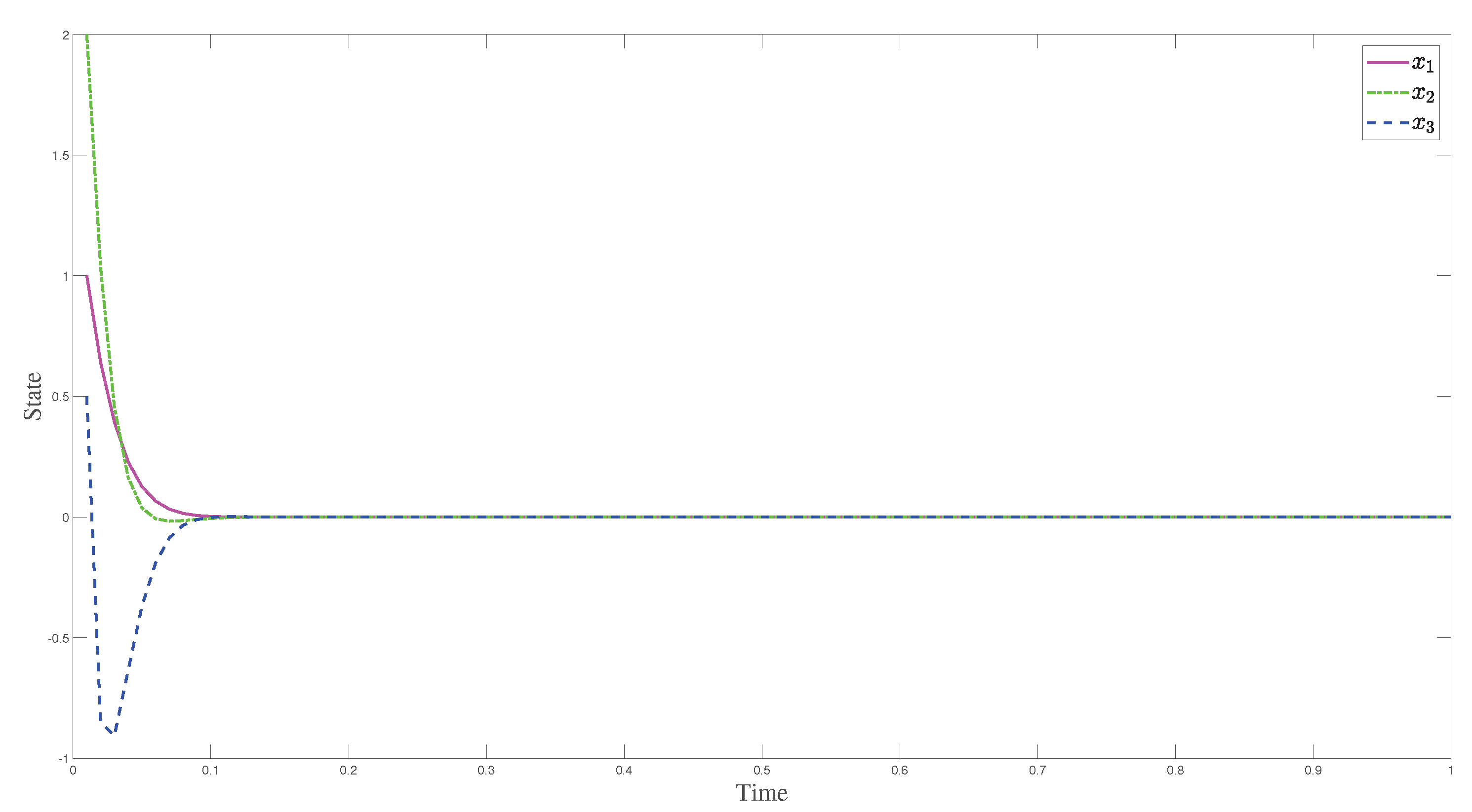
The sampling period T = 0.01 is first selected in the fractional difference approximation of differentiation when α = 0.5 in this section. For the simplicity of analysis, k 1 = 1 , k 2 = 3 , k 3 = 1 was used in the following studies.
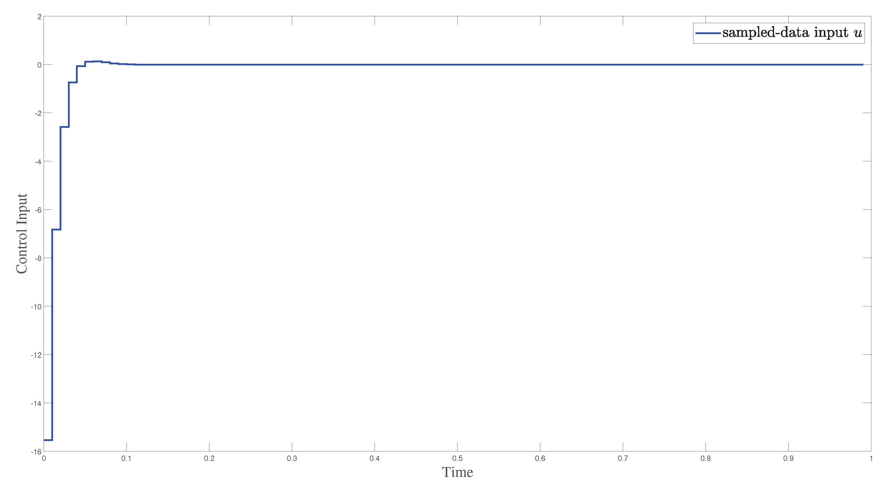
Simulation results under initial conditions ( 1 , 2 , 0.5 ) T and scaling gain L = 2 are presented in Figure 2 and Figure 3, where the asymptotic stability of system (14) was realized under the sampled-data controller (15).

4.2. Sampled-Data Stabilization under Large Sampling Period

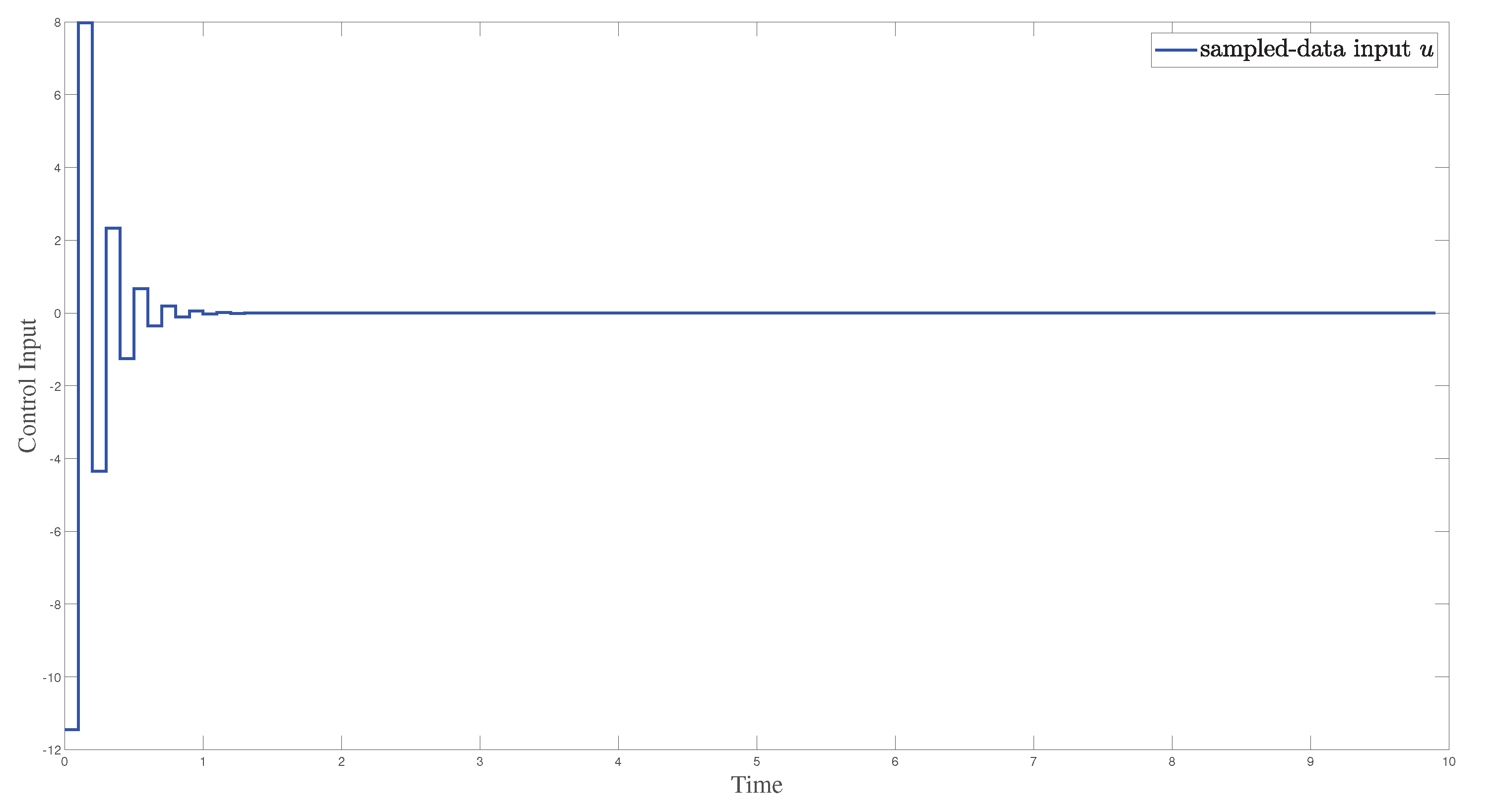
To show the advantages endowed by the sampled-data controller (15), simulation studies under both the sampling period T = 0.1 and T = 1 were conducted in this section, wherein all the other settings are the same as that in the previous Section 4.1.
Because the sampling period increased from T = 0.01 to T = 0.1 and T = 1 in the following studies, L = 1.5 and L = 0.15 were selected, respectively, in this case, for the purpose of the stability of the closed-loop system. Under controller (15) and the sampling period T = 0.01 and T = 0.1 , the states of system (14) with respect to time were presented in Figure 4 and Figure 5, while the control input under the sampled-data controller (15) was shown in Figure 6 and Figure 7. The obtained results have illustrated the effectiveness of the co-designed sampled-data controller (15) even when the sampling period is greatly increased which is much preferred in the digital implementation of obtained sampled-data controllers.
Remark 5.
Comparisons of simulation results under different sampling periods show that the more the sampling period increases, the longer the settling time becomes, and the bigger the overshoot increases, which is a consequence of compensation between the scaling gain and sampling period.
Remark 6.
Only the most recent sampling information x ( k T ) was used in the above simulation studies. Based on the results obtained, there are a lot of interesting extensions such as the sampled-data stabilization of the fractional linear system (1) using the oldest information x ( T ) , as shown in Corollary 1.

4.3. Sampled-Data Stabilization Using the Oldest Information

The following sampled-data controller based on the most old information x ( T )
u ( t ) = L 3 α k 1 x 1 ( T ) L 2 α k 2 x 2 ( T ) L α k 3 x 3 ( T ) ,   for t [ T , ( k + 1 ) T )
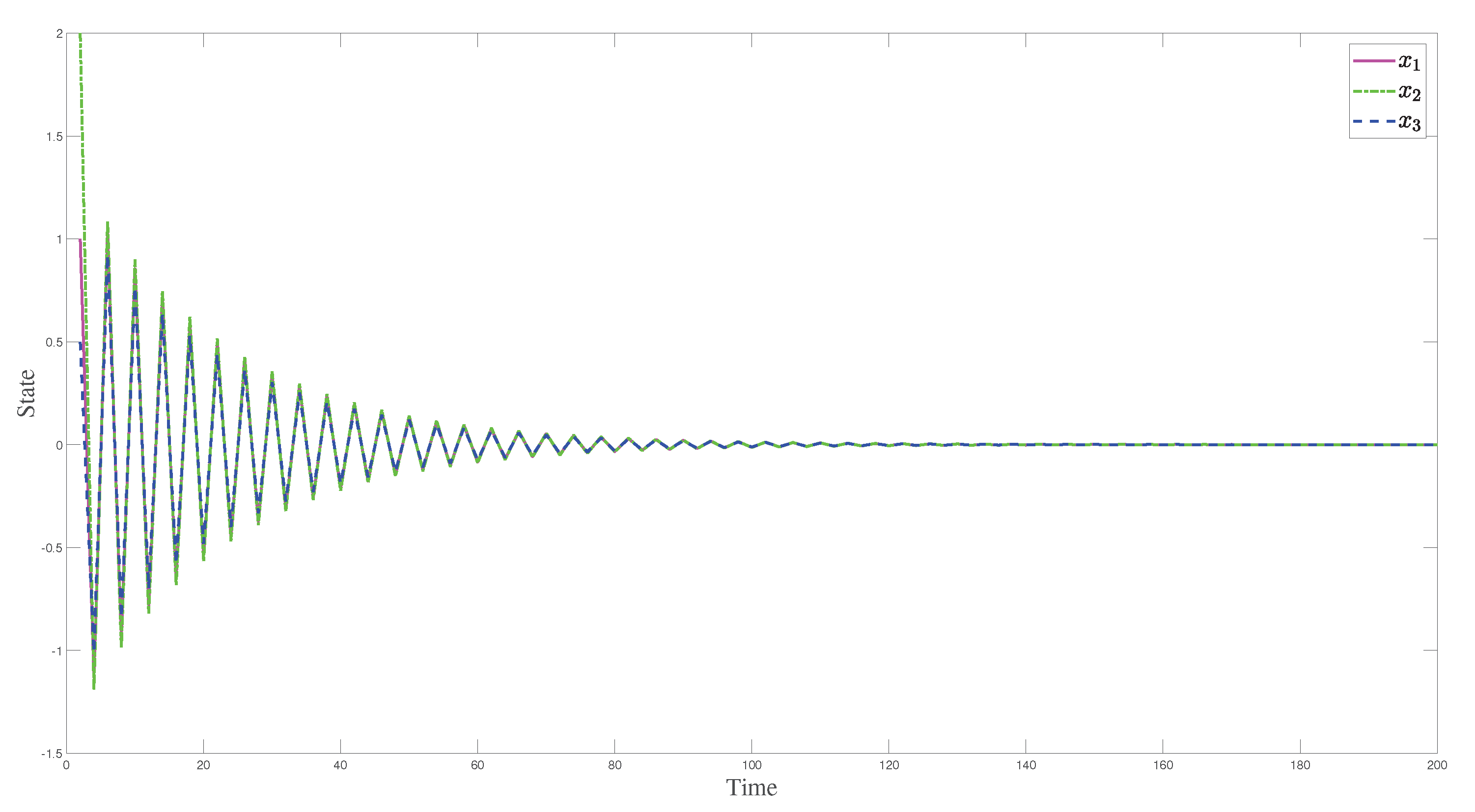
was employed in the following simulation studies to illustrate the main results shown in Corollary 1. Because only the oldest information of x ( T ) was used to update the controller, the whole control system acts as a system with an expanded sampling period, where the computation burden in the digital implementation of obtained controllers can be relieved in some sense. Similarly to the sample-data control with large sampling periods in the previous section, sampled-data stabilization can also be realized under the compensation of scaling gain.
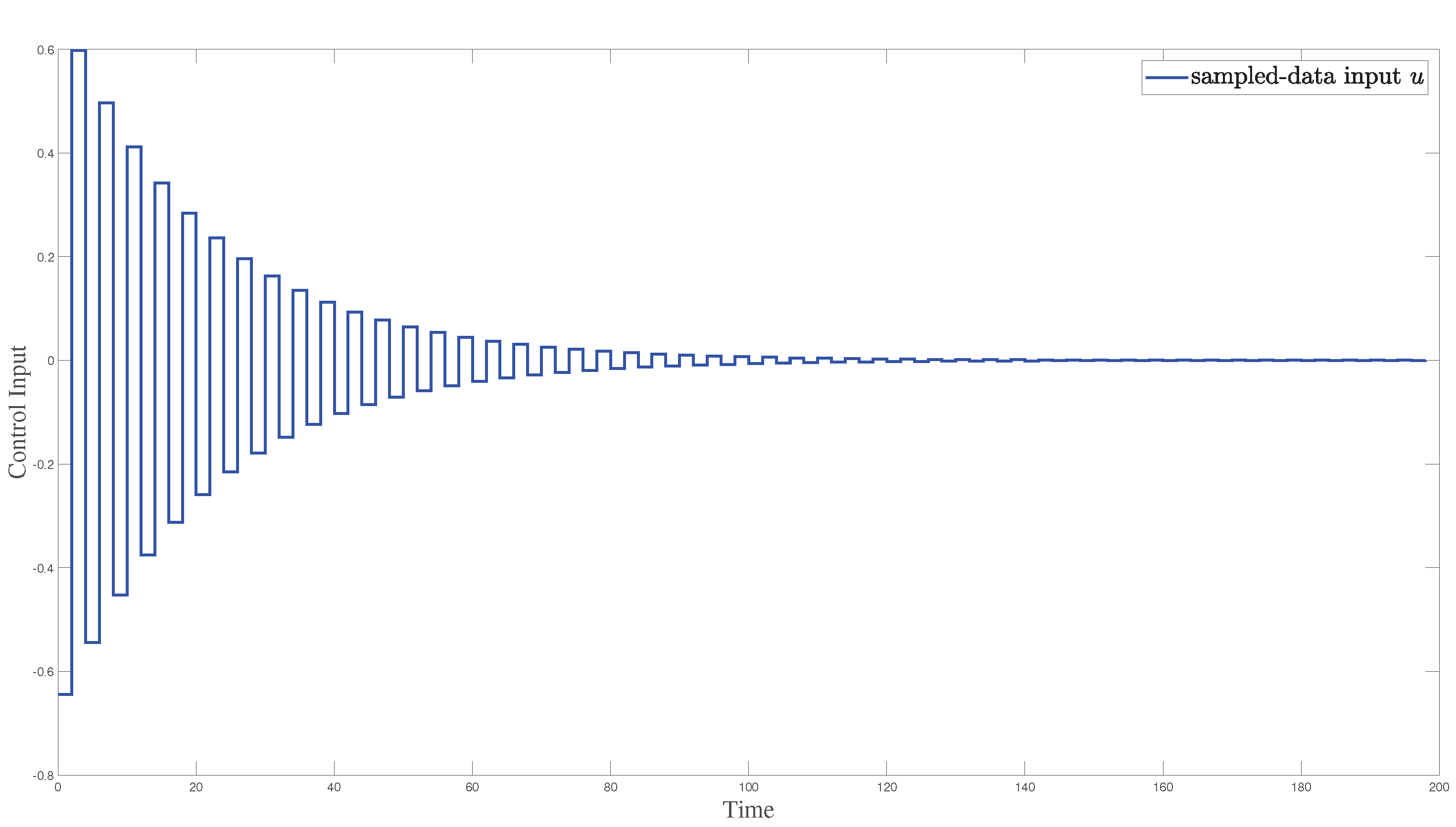
For the clarity of comparison, T = 2 was selected in the following simulation studies where the states of system (14) with respect to time were presented in Figure 8 while the sample-data input with respect to time are presented in Figure 9. The obtained results show the possibility of stabilizing the system (14) using the “oldest” information using the sampled-data controller (16) proposed in corollary 1.

5. Conclusions

The sampled-data stabilization of a fractional linear continuous system was studied under arbitrary sampling periods based on compensation between the scaling gain and sampling period in this paper. Sufficient and necessary conditions for the stability of a fractional linear system are first presented in terms of scaling gain, sampling period and system matrix. Then, co-designed sampled-data controllers are directly constructed in the discrete-time domain where not only the “newest” state but also the “oldest” state can be utilized in the sampled-data stabilization of the fractional linear system. Additionally, much more flexibility on selecting different sampling periods was provided in sampled-data stabilization using the co-designed controllers proposed. Simulation results under different sampling periods are also presented to illustrate the effectiveness of the obtained results.
Based on the obtained results, there are a lot of interesting topics worthy of much more effort such as the further extension to a nonlinear system of fractional order or constructing the sampled-data output feedback controller for the stabilization of a system of fractional order.

Author Contributions

Conceptualization, writing—original draft preparation and software: K.C.; supervision, validation and project administration: J.G.; software and validation: J.M.; software and validation: C.L. All authors have read and agreed to the published version of the manuscript.

Funding

This research was funded by the National Natural Science Foundation of China (Grant No. 61973178, 61973139, Key Program: u2066203), The Key Project of Philosophy and Social Science Research in Colleges and Universities in Jiangsu Province (Grant No. 2020SJZDA098), Startup Foundation for Introduced Talents of Nanjing Institute of Technology (Grant No. YKJ202016). The APC was funded by 2020SJZDA098, YKJ202016.

Institutional Review Board Statement

Not applicable.

Informed Consent Statement

Not applicable.

Data Availability Statement

Not applicable.

Conflicts of Interest

The authors declare no conflict of interest.

References

  1. Podlubny, I. Fractional Differential Equations; Academic Press: San Diego, CA, USA, 1999. [Google Scholar]
  2. Tarasov, V.E. Review of Some Promising Fractional Physical Models. Int. J. Mod. Phys. B 2013, 27, 1–32. [Google Scholar] [CrossRef] [Green Version]
  3. Sunny, M.R.; Kapania, R.K.; Moffitt, R.D.; Mishra, A.; Goulbourne, N. A Modified Fractional Calculus Approach to Model Hysteresis. J. Appl. Mech. 2010, 77, 031004. [Google Scholar] [CrossRef]
  4. Zhang, X. Relationship between integer order systems and fractional order system and its two applications. IEEE/CAA J. Autom. Sin. 2018, 5, 639–643. [Google Scholar] [CrossRef]
  5. Luo, Y.; Chen, Y. Fractional Order Motion Controls; John Wiley & Sons, Ltd., Publication: Chichester, UK, 2012. [Google Scholar]
  6. Petras, I. Fractional-Order Nonlinear Systems Modeling, Analysis and Simulation; Springer: Berlin/Heidelberg, Germany, 2011. [Google Scholar]
  7. Rajagopal, A.; Hasanzadeh, N.; Parastesh, F.; Hamarash, I.I.; Jafari, S.; Hussain, I. A fractional-order model for the novel coronavirus (COVID-19) outbreak. Nonlinear Dyn. 2020, 101, 711–718. [Google Scholar] [CrossRef] [PubMed]
  8. Cao, K.; Chen, Y.; Stuart, D. A fractional micro-macro model for crowds of pedestrians based on fractional mean field games. IEEE/CAA J. Autom. Sin. 2016, 3, 261–270. [Google Scholar]
  9. Arshad, S.; Sohail, A.; Javed, S. Dynamical Study of Fractional Order Tumor Model. Int. J. Comput. Methods 2015, 12, 1550032. [Google Scholar] [CrossRef]
  10. Edet, E.; Katebi, R. On Fractional-order PID Controllers. IFAC-PapersOnLine 2018, 51, 739–744. [Google Scholar] [CrossRef]
  11. Shah, P.; Agashe, S. Review of fractional PID controller. Mechatronics 2016, 38, 29–41. [Google Scholar] [CrossRef]
  12. Zhang, X.; Huang, W.; Wang, Q.G. Robust H Adaptive Sliding Mode Fault Tolerant Control for T-S Fuzzy Fractional Order Systems with Mismatched Disturbances. IEEE Trans. Circuits Syst. I Regul. Pap. 2021, 68, 1297–1307. [Google Scholar] [CrossRef]
  13. Zhang, X.; Huang, W. Adaptive Neural Network Sliding Mode Control for Nonlinear Singular Fractional Order Systems with Mismatched Uncertainties. Fractal Fract. 2020, 4, 50. [Google Scholar] [CrossRef]
  14. Gao, Z.; Liao, X.Z. A stability criterion for linear fractional order systems in frequency domain. Zidonghua Xuebao/Acta Autom. Sin. 2011, 37, 1387–1394. [Google Scholar]
  15. Zhang, X.; Lin, C.; Chen, Y.Q.; Boutat, D. A Unified Framework of Stability Theorems for LTI Fractional Order Systems with 0 < α < 2. IEEE Trans. Circuits Syst. II Express Briefs 2020, 67, 3237–3241. [Google Scholar]
  16. Bohner, M.; Tunç, O.; Tunç, C. Qualitative analysis of caputo fractional integro-differential equations with constant delays. Comput. Appl. Math. 2021, 40, 1–17. [Google Scholar] [CrossRef]
  17. Yang, Q.; Chen, D.; Zhao, T.; Chen, Y. Fractional calculus in image processing: A review. Fract. Calc. Appl. Anal. 2016, 19, 1222–1249. [Google Scholar] [CrossRef] [Green Version]
  18. Gardner, S.A. Exploring Fractional Order Calculus as an Artificial Neural Network Augmentation. Master’s Thesis, Montana State University, Bozeman, MT, USA, 2009. [Google Scholar]
  19. Pan, I.; Saptarshi, S. Applied fractional calculus for computational intelligence researchers. In Intelligent Fractional Order Systems and Control: An Introduction; Springer: Berlin/Heidelberg, Germany, 2013; pp. 9–61. [Google Scholar]
  20. Åström, K.J.; Wittenmark, B. Computer-Controlled Systems: Theory and Design; Prentice Hall: Hoboken, NJ, USA, 1997. [Google Scholar]
  21. Dzieliński, A.; Sierociuk, D. Stability of Discrete Fractional Order State-space Systems. J. Vib. Control. 2008, 14, 1543–1556. [Google Scholar] [CrossRef]
  22. Liu, T.; Wei, Y.; Yin, W.; Wang, Y.; Liang, Q. State estimation for nonlinear discrete-time fractional systems: A Bayesian perspective. Signal Process. 2019, 165, 250–261. [Google Scholar] [CrossRef]
  23. Yuan, X.; Mo, L.; Yu, Y.; Ren, G. Containment control of fractional discrete-time multi-agent systems with nonconvex constraints. Appl. Math. Comput. 2021, 409, 126378. [Google Scholar] [CrossRef]
  24. Cao, J.; Chen, Y.; Li, C. Multi-UAV-based Optimal Crop-dusting of Anomalously Diffusing Infestation of Crops. In Proceedings of the American Control Conference, Chicago, IL, USA, 1–3 July 2015; pp. 1278–1283. [Google Scholar]
  25. Chen, Y.; Xue, D.; Dou, H. Fractional Calculus and Biomimetic Control. In Proceedings of the IEEE International Conference on Robotics and Biomimetics (RoBio04), Shenyang, China, 22–26 August 2004; pp. 901–906. [Google Scholar]
  26. Abdelaziz, M.A.M.; Ismail, A.I.; Abdullah, F.A.; Mohd, M.H. Discrete-Time Fractional Order SIR Epidemic Model with Saturated Treatment Function. Int. J. Nonlinear Sci. Numer. Simul. 2020, 21, 397–424. [Google Scholar] [CrossRef]
  27. Stanislawski, R.; Latawiec, K.J. Normalized finite fractional differences: Computational and accuracy breakthroughs. Int. J. Appl. Math. Comput. Sci. 2012, 22, 907–919. [Google Scholar] [CrossRef]
  28. Shahamatkhah, E.; Tabatabaei, M. Leader-following consensus of discrete-time fractional-order multi-agent systems. Chin. Phys. B 2018, 27, 010701. [Google Scholar] [CrossRef] [Green Version]
  29. Yu, Z.; Jiang, H.; Hu, C.; Yu, J. Necessary and Sufficient Conditions for Consensus of Fractional-Order Multiagent Systems via Sampled-Data Control. IEEE Trans. Cybern. 2017, 47, 1892–1901. [Google Scholar] [CrossRef] [PubMed]
  30. Cao, K.; Qian, C.; Gu, J. Sampled-data control of a class of uncertain nonlinear systems based on direct method. Syst. Control. Lett. 2021, 155, 105000. [Google Scholar] [CrossRef]
  31. Monje, C.A.; Chen, Y.; Vinagre, B.M.; Xue, D.; Feliu, V. Fractional Order Systems and Controls: Fundamentals and Applications; Springer: London, UK, 2010. [Google Scholar]
  32. Miller, K.S.; Ross, B. An Introduction to the Fractional Calculus and Fractional Differential Equations; John Wiley & Sons: New York, NY, USA, 1993. [Google Scholar]
  33. Stanislawski, R.; Latawiec, K.J. Stability analysis for discrete-time fractional-order LTI state-space systems. Part I: New necessary and sufficient conditions for the asymptotic stability. Bull. Pol. Acad. Sci. Tech. Sci. 2013, 61, 353–361. [Google Scholar] [CrossRef] [Green Version]
  34. Cao, K.; Qian, C.; Gu, J.; Hua, L. Co-designed sampled-data output consensus for multi-agent systems. Int. J. Robust Nonlinear Control. 2021, 31, 5762–5775. [Google Scholar] [CrossRef]
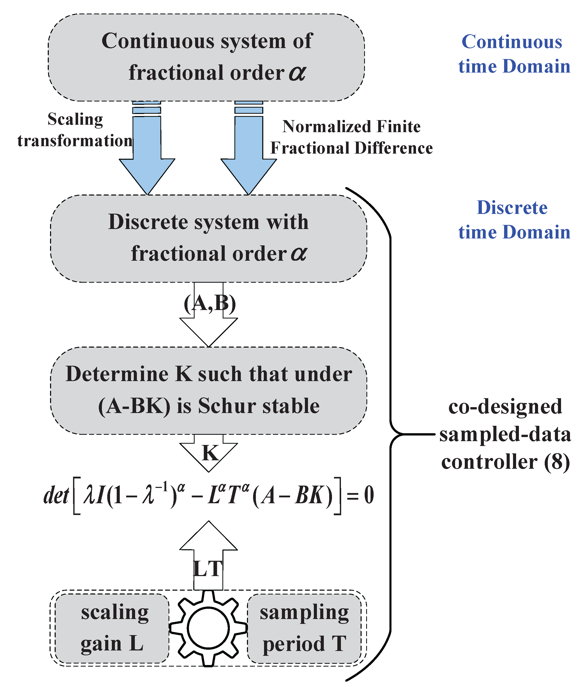
Figure 1. Procedure of identifying the parameters in the co-designed sampled-data controller (8).
Fractalfract 06 00416 g001
Figure 2. States of system (14) with respect to time under controller (15) with T = 0.01 .
Fractalfract 06 00416 g002
Figure 3. Sampled–datainput of system (14) in function of the time under controller (15) and T = 0.01 .
Fractalfract 06 00416 g003
Figure 4. States of system (14) with respect to time under controller (15) with T = 0.1 .
Fractalfract 06 00416 g004
Figure 5. States of system (14) with respect to the time under controller (15) with T = 1 .
Fractalfract 06 00416 g005
Figure 6. Sampled–data input of system (14) in function of the time under controller (15) and T = 0.1 .
Fractalfract 06 00416 g006
Figure 7. Sampled–data input of system (14) in function of the time under controller (15) and T = 1 .
Fractalfract 06 00416 g007
Figure 8. States of system (14) with respect to time under controller (16) with T = 2 .
Fractalfract 06 00416 g008
Figure 9. Sampled–data input of system (14) in function of time under controller (16) and T = 2 .
Fractalfract 06 00416 g009
Publisher’s Note: MDPI stays neutral with regard to jurisdictional claims in published maps and institutional affiliations.