Article

Ensemble FARIMA Prediction with Stable Infinite Variance Innovations for Supermarket Energy Consumption

1
School of Electrical and Control Engineering, North China University of Technology, Beijing 100144, China
2
College of Information Science and Technology, Beijing University of Chemical Technology, Beijing 100029, China
3
Institute of Intelligence Science and Engineering, Shenzhen Polytechnic, Shenzhen 518055, China
*
Authors to whom correspondence should be addressed.
Fractal Fract. 2022, 6(5), 276; https://doi.org/10.3390/fractalfract6050276
Submission received: 11 April 2022 / Revised: 19 May 2022 / Accepted: 20 May 2022 / Published: 22 May 2022

Abstract

:
This paper concerns a fractional modeling and prediction method directly oriented toward an industrial time series with obvious non-Gaussian features. The hidden long-range dependence and the multifractal property are extracted to determine the fractional order. A fractional autoregressive integrated moving average model (FARIMA) is then proposed considering innovations with stable infinite variance. The existence and convergence of the model solutions are discussed in depth. Ensemble learning with an autoregressive moving average model (ARMA) is used to further improve upon accuracy and generalization. The proposed method is used to predict the energy consumption in a real cooling system, and superior prediction results are obtained.

1. Introduction

The modern industrial process exhibits complex dynamic behavior due to its strong nonlinearity, disturbance, and coupling. In general, the industrial data are non-normally distributed. However, traditional data analysis methods usually assume that the data is subject to a Gaussian distribution. Therefore, pre-transformation from non-Gaussian to Gaussian should be considered, such as logarithmic transformation [1], Box-Cox transformation [2], exponential transformation, and reciprocal transformation. The normalizing transformations inevitably remove many important hidden features from the raw data. To avoid the loss caused by normalizing transformation, a new probability distribution is proposed to describe non-Gaussian information directly, e.g., as a α -stable distribution, a skewed distribution, and higher-order statistics [3,4]. An α -stable distribution can describe a random signal with a strong spike pulse and a thick trailing feature, such as a medical signal, an industrial process variable [5], a radar signal [6], and gene expression data [7]. It also has applications in complex system control [8,9,10,11] and image processing [12,13,14]. A α -stable distribution better captures the nature of data compared to a Gaussian distribution in many applications [15].
An industrial time series usually does not satisfy the assumption of a Gaussian normal distribution. Due to the process complexity, it always includes many nonlinear or non-Gaussian features, such as a heavy tail [16], self-similarity [17], and long-range dependence [18]. These behaviors are classified as typical fractional order features. Therefore, aiming at a non-normal industrial time series, data analytics directly in the frame of fractional order theory is becoming an important issue.
Long-range dependence (LRD) is a typical fractional order characteristic widespread in complex systems, such as hydrological observations [19], traffic networks [20], and financial fields [21]. A stationary process has LRD if its autocorrelations hardly decay to zero even across large time scales [22,23]. LRD is evaluated by a self-similarity parameter, the Hurst exponent [24,25]. There are many techniques used to calculate the Hurst exponent, such as the rescaled range method (R/S), the whittle estimator method, and the absolute value method. Likewise, fractal theory is also important for analyzing fractional order characteristics [26,27]. It reflects the structural similarities across the whole time series, which further affects its stationarity. The detrended fluctuation analysis method (DFA) is popular in fractal theory [28]. It is used to evaluate the non-stationarity and long-range dependence of time series [29]. Multifractal detrended fluctuation analysis (MFDFA) was proposed to eliminate trends and retain the fluctuation component [30,31]. It is more suitable for the scale characteristic analysis of time series.
LRD and fractal features describe the trends of variables and help to accurately predict time series [5]. In fact, many prediction models have been proposed in recent decades, such as the autoregressive integrated moving average model (ARIMA) [32], tensor product (TP)-based model transformation [33], the self-healing neural model [34], the long short-term memory model [35,36], and other randomized learning neural networks [37]. These models show good performance for nonlinear systems. Many practical processes can be described more accurately when fractional differential equations are introduced. For example, the authors in [5] proposed a fractional stochastic configuration network to model the nonstationary time series, and better potential prediction performance was obtained compared with the modeling methods only for the stationary variable. The authors in [38] analyzed the relationship between an integer order system and a fractional order system in depth.
In this paper, a fractional autoregressive integrated moving average model (FARIMA) is used to predict an industrial time series with obvious fractional features [39,40]. FARIMA is an improvement over ARIMA that overcomes the excessive difference in data. Moreover, the ensemble learning strategy is proposed to further improve prediction accuracy [41,42]. It combines the prediction results of different models through voting, averaging, and stacking strategies. It takes advantage of different learning models and improves the generalization of the prediction model simultaneously.
The contributions of this paper are as follows:
(1) FARIMA is proposed to forecast the industrial time series with stable infinite variance, and the existence and convergence of model solution are also analyzed.
(2) An ensemble FARIMA is proposed to improve prediction accuracy and generalization, and the hidden fractional features, the LRD, and the multifractal property are mined.
(3) The proposed method is applied to predict the energy consumption of a supermarket cooling system, and the effectiveness and accuracy are verified.
This paper is structured as follows: Section 2 presents the FARIMA model, including an analysis about the existence and convergence of the model solution. Section 3 presents the framework of fractional analytics and the extraction of fractional features hidden in the industrial process. Section 4 uses the proposed method to predict energy consumption for an actual cooling system. Finally, Section 5 presents the conclusions.

2. The FARIMA Model

Many signals are non-stationary in industrial systems due to the uncertain disturbance. The fractional autoregressive integrated moving average (FARIMA) model can flexibly simulate this random process full of fraction order signals. The basic structure of FARIMA is as follows:
Φ ( B ) ( 1 B ) d Y t = Θ ( B ) X t ,
where d ( 0 , 1 ) is positive and real. Note that Equation (1) also represents an ARIMA model with d = 0 and an ARIMA model with d = 1 .
The input or innovation X t is independent and identically distributed (i.i.d.) with infinite variance. B is the delay operator, defined by B Y t = Y t 1 , such that ( 1 B ) d represents a nabla fractional derivative of order d [43,44]. Φ B and Θ B are p order autoregression polynomials and q order moving average polynomials, respectively, which are defined as Φ B = 1 ϕ 1 B 1 ϕ 2 B 2 ϕ p B p and Θ B = 1 + θ 1 B 1 + θ 2 B 2 + + θ q B q .
Let’s move ( 1 B ) d and Φ B of Formula (1) from the left to the right,
Y t = Θ ( B ) Φ ( B ) ( 1 B ) d X t
Throughout this paper, we assume the following.
Assumption 1.
The autoregression polynomials Φ B and moving average polynomials Θ B have no roots in common, nor does Φ B have roots in the closed unit disk { B : | B | 1 } .
Assumption 2.
The input or innovation X t is an i.i.d. symmetric α-stable ( S α S ) random distribution with 0 < α 2 .
Remark 1.
Assumption 1 guarantees that the coefficients of Θ ( B ) Φ ( B ) tend exponentially towards zero and that FARIMA time series are causal moving averages. Assumption 2 indicates the distribution of the innovation X t , in which 0 < α < 2 corresponds with fractional d, and α = 2 indicates a Gaussian distribution. An explanation of a symmetric α-stable distribution is given in Section 3.2.
The linear solution of the FARIMA model, Equation (2), takes the form of a time series as follows:
Y t = j = 0 a j X t j
where a j is defined as
A d ( B ) Θ ( B ) Φ ( B ) ( 1 B ) d = j = 0 a j B j , | B | < 1
The authors in [45,46] provided a solution to the FARIMA model with finite variance innovations. They indicated that the solutions in Equations (3) and (4) converge a.s. if and only if j | a j | α < , but this condition cannot guarantee absolute convergence if α > 1 . Moreover, this condition would not allow positive values of a fractional d when α 1 , which means that only the negative values of d are admissible. The authors of [47] considered the fact that variance does not exist (i.e., infinite variance) for S α S random variables with 0 < α < 2 , which are ubiquitous in the industrial system. They studied the existence and convergence of a FARIMA solution under the condition of stable infinite variance innovations.
Theorem 1
(Existence). If α ( d 1 ) < 1 , then the sequence Y t given in Equations (3) and (4) is the unique causal moving average solution of the FARIMA model, Equation (2).
Theorem 1 discusses the existence of a unique causal moving average solution to FARIMA under the condition α ( d 1 ) < 1 . It implies that d is negative if a 1 . In order to extend the constraint for fractional d, a considerable flexibility in manipulating function of the operation B is introduced.
Theorem 2
(Considerable Flexible Existence). Suppose { X t } is a sequence of i.i.d. S α S random variables with 0 < α 2 . Let a j , j = 0 , 1 , be a sequence of real numbers satisfying j | a j | α < . Let λ j , j = 0 , 1 , be a sequence of real numbers satisfying
j | λ j | α < , i f α 1 j | λ j | < , i f α > 1
If Y t : = j = 0 a j X t j , Λ t : = j = 0 λ j X t j and C ( B ) X t : = j = 0 c j X t j with c j = k = 0 j λ k a j k , then
lim m k = 0 m λ k Y t k = j = 0 c j X t j
lim s k = 0 s a k Λ t k = j = 0 c j X t j
where convergence is in the L p n o r m for any 0 < p < α . Moreover, the left-hand side of Equation (6) converges absolutely a.s. for α > 1 . Moreover, when α 1 , it is an absolute a.s. convergence under the additional condition j | λ j | r < , for some 0 < r < α .
Based on Theorem 2, the moving average polynomial Θ ( B ) can be factored into a product of two polynominals as Θ ( B ) = Θ 1 ( B ) Θ 2 ( B ) . The FARIMA model, Equation (2), is then rewritten as
Θ 1 1 ( B ) Y t = Θ 2 ( B ) Φ ( B ) ( 1 B ) d X t a . s .
For any non-negative integer r, we have ( 1 B ) r A d ( B ) = A d r ( B ) . Comparing Equations (2) and (8) implies ( 1 B ) r Y t d = Y t d r a . s . from Theorem 2. Therefore, any FARIMA model ( p , d , q ) can be equivalent to a FARIMA model ( p , d ¯ , q ) with d ¯ [ 1 α , 1 1 α ] . Furthermore, Theorem 2 verifies that S α S FARIMA is invertible if 1 < α 2 and | d | < 1 1 α , which means the further convergence of the FARIMA solution.
Theorem 3
(Convergence). Suppose Y t = j = 0 a j X t j , Equation (3), where coefficient a j , Equation (4), is the solution of the FARIMA, Equation (2). If | d | < 1 1 α , then, for any 0 < p < α ,
lim m E | k = 0 m a ˜ k Y t k X t | p = 0
with the coefficients a ˜ k defined as
A d 1 ( B ) Φ ( B ) Θ ( B ) ( 1 B ) d = j = 0 a ˜ j B j , B < 1
Moreover, for | d | < 1 1 α , the partial sums k = 0 m c ˜ k Y t k converge to X t absolutely a.s.
It is noted that the proofs for Theorems 1–3 is omitted for simplification. They are similar to those of [47], which presented the proofs in detail.
The implementation of FARIMA consists of a fractional derivative operation and ARMA regression. Consider that a raw series Y t and a corresponding series W t are obtained after a fractional d order derivative operation:
W t = ( 1 B ) d Y t
The fractional order d = H 0.5 usually is determined by the Hurst exponent. The binomial term ( 1 B ) d represents the fractional nabla derivative,
( 1 B ) d = T d k = 0 ( d ) k k ! B k
where T is the sampling interval, and ( d ) k is the Pochhammer representation of the rising factorial, such that ( d ) 0 = 1 and ( d ) k = i = 0 k 1 ( d + i ) . Define f ( k ) T d ( d ) k k ! for known order d. Equation (11) is then expressed as
W t = k = 0 f ( k ) B k Y t = f ( 0 ) Y t + f ( 1 ) Y t 1 + f ( 2 ) Y t 2 + + f ( k ) Y t k +
Assume Y t = 0 for all t ( , 0 ] without a loss of generality
  • when t = 0 , Y 0 = 0 , W 0 = 0 ;
  • when t = 1 , W 1 = f ( 0 ) Y 1 + f ( 1 ) Y 0 = f ( 0 ) Y 1 ;
  • when t = 2 , W 2 = f ( 0 ) Y 2 + f ( 1 ) Y 1 ;
  • when t = 3 , W 3 = f ( 0 ) Y 3 + f ( 1 ) Y 2 + f ( 2 ) Y 1 ;
  • when t = N , W N = f ( 0 ) Y N + f ( 1 ) Y N 1 + f ( 2 ) Y N 2 + + f ( N ) Y 1 .
Formula (11) is then rewritten as matrices:
W = Y T F
where W = W 1 W 2 W N , Y = Y 1 Y 2 Y N and
F = f ( 0 ) f ( 1 ) f ( 2 ) f ( 3 ) f ( N 1 ) f ( 0 ) f ( 1 ) f ( 2 ) f ( N 2 ) f ( 0 ) f ( 1 ) f ( 2 ) f ( 0 ) f ( 1 ) f ( 0 )
Once the fractional series W t is calculated from Equation (14), the ARMA model is directly performed on it. The ARMA parameters p , q are determined by the autocorrelation function (ACF) and partial autocorrelation function (PACF). The Akaike information criterion (AIC) is used to evaluate the accuracy of p and q [48]. The residual is then calculated and tested by white Gaussian noise in order to verify the fitness of the ARMA model.
The ARMA model accurately captures the system features only when the process data are stationary and follow a Gaussian distribution. However, these conditions have not been met in a real industrial signal, so a fractional derivative is first adopted to eliminate the non-stationary characteristics. In general, a fractional derivative can more delicately depict the key features hidden in an industrial time series than an integer difference.

3. Fractional Analytics for Industrial Data

3.1. General Framework

Reliable and comprehensive analytics for industrial data can greatly improve process production. An actual industrial process is inevitably accompanied by all kinds of disturbances and random events, such as power outages and system failures. These factors lead to typical fractional characteristics in time series, such as power laws, trends, self-similarity, and long-range dependence.
Here, a methodology used to analyze time series with fractional properties is shown in Figure 1. The data features, including the LRD and self-similarity, are first extracted using the Hurst exponent and fractal theory. If they exhibit an obvious fractional behavior, FARIMA modeling and prediction should be completed under the frame of fractional analytics. However, if the data fits into a normal distribution, traditional analysis methods and forecasting models should be developed.

3.2. Fractional Feature Extraction

Here, we introduce several mathematic techniques to extract the fractional feature hidden in the time series.
α -stable distribution Traditional data processing assumes that the data fit as a Gaussian distribution due to its ease of analysis. Many methods can transform non-Gaussian data into a Gaussian distribution. However, the problem is that the process information carried by the raw data may be lost in the transformation. Therefore, it is important to analyze raw non-Gaussian information in data analysis. For this reason, an α -stable distribution can be employed to describe non-Gaussian signals. The characteristic function of an α -stable distribution is given as follows:
Φ ( t ) = exp j δ t γ | t | α [ 1 + j β sign ( t ) ω ( t , α ) ]
where 0 < α 2 , 1 β 1 , γ > 0 , and
ω ( t , α ) = tan α π 2 , if α 1 2 π log | t | , if α = 1 sign ( t ) = 1 , if t > 0 0 , if t = 0 1 , if t < 0
The shape of an α -stable distribution depends on four parameters: α , β , γ , δ . α represents the tail features of the distribution with high relevance when 0 < α < 2 . When α = 2 , an α -stable distribution is equal to a Gaussian distribution. β is the coefficient of skewness. β = 0 means that the distribution is symmetric. 1 β < 0 and 0 < β 1 imply that the distribution is left-skewed or right-skewed, respectively. γ is the scale coefficient, which is similar to the variance of the Gaussian. The data are dispersed when γ is large. δ is the location parameter. It is the median if 0 < α < 1 or the average if 1 α < 2 , for a symmetric distribution (i.e., β = 0 ).
The existence of order statistics moments in a distribution is important for parameter estimation. The sufficient and necessary conditions for the existence of moments of an α -stable distribution are given in [49,50]. The location parameter δ and scale parameter γ have no influence on the existence of moments, and the influence of the skewness parameter β is almost negligible compared with the tail parameter α . Based on the existence conditions, all parameters of an α -stable distribution can be estimated. The density function is firstly calculated according to the characteristic function (1) by fast Fourier transform or integral transform. The parameter estimation problem is then transformed into error minimization between the density function and the probability density function of raw data.
LRD and Hurst exponent An LRD is a typical non-Gaussian behavior always accompanying the industrial processes. It denotes the autocorrelation of time series and is important for trend forecasts. The Hurst exponent is a measurement of how the range of fluctuations in a time series varies with the time span. It is a common tool for analyzing LRD features. The definition of the Hurst exponent are interpreted in the time domain and the frequency domain. Here, we use its definition in the time domain:
E [ R ( n ) S ( n ) ] n = C n H
where E is the mean value, R is the range, S is the standard deviation, C is the constant, H is the Hurst exponent, and H ( 0 , 1 ) . Specifically, if H > 0.5 , the change trend of the process variable is the same as it was in the past; if H < 0.5 , the trend is opposite to what it was in the past. If H = 0.5 , the process variable is a random walk, which means that the change in the future has no relation to the past.
The calculation of the Hurst exponent is achieved by the rescaled range method (R/S) [51,52]. Consider the time series X t , t = 1 , , N . First, it is equally divided it into m subsequences and is denoted as D a , a = 1 , , m . The length of each subsequence D a is n ( m = N / n is an integer). For each subsequence D a and its samples X j , a D a , j = 1 , , n , its mean value X a ¯ , cumulative deviation Y j , a , standard deviation S a , and range R a are calculated.
X a ¯ = 1 n j = 1 n X j , a Y j , a = i = 1 n X j , a X ¯ a S a = 1 n j = 1 n X j , a X ¯ a 2 R a = max 1 j n Y j , a min 1 j n Y j , a
The rescaled range ( R / S ) a of subsequence D a and its mean value at the given subsequence length n are
( R / S ) a = R a / S a ( R / S ) n = ( 1 / m ) a = 1 m ( R / S ) a
Let the length n of subsequence increase from 2 until n = N / 2 and calculate all ( R / S ) n for all n = 2 , , N / 2 . Consider the following form F ( τ ) = ( R / S ) n = C τ H , where C is a constant and H is the Hurst exponent. Taking the logarithm on it, we have
log F ( τ ) = log C + H log τ
The least square method is used to obtain the regression equation, Equation (19), and the Hurst exponent H.
Multifractal analysis Self-similarity is a property maintained when scaling in time or space. Due to the homogeneous nature of continuous process products, self-similarity is widely found in the industrial process. Fractal theory usually describes the self-similarity of time series, and the fractal dimension is a measurement of fractal complexity to evaluate the validity of space occupied and the irregularity. The quantitative index for fractal dimension is given as follows:
D = ln K ln L
where L is the magnification factor of the geometry object, K is the total number of self-similar objects needed to form a complex one, and D is the fractal dimension. There are many methods used to calculate the fractal dimension and are applied in many fields. A central method, multifractal detrended fluctuation analysis (MFDFA), is often used to characterize the variability and uncertainty for time series [53,54]. MFDFA accurately estimates the fractal characteristics of unstable data, so it has been successfully used in many fields.
For time series X t , its cumulative deviation is
Y ( j ) = i = 1 j X t X ¯ , t = 1 , 2 , 3 , , N
where X ¯ is the mean value of raw time series. The sequence is divided into isometric intervals of length s, and the number N s of subinterval v can be expressed as N s = int N s , where int is rounded down. N is not necessarily divisible by s in practice, and some tail data may thrown away. Therefore, we start from the tail of the sequence and divide it forward again in order to ensure the integrity of the information and obtain the 2 N s subinterval.
The least square method is adopted to fit the polynomial with order k for each subinterval v ( v = 1 , 2 , , 2 N s ), and the local trend function is obtained,
Y v ( j ) = a 0 + a 1 j + a 2 j 2 + + a k j k
where a k is the coefficient of the polynomial, and k is the highest coefficient of the polynomial.
The trend is eliminated by calculating the mean variance F 2 ( v , s ) :
F 2 ( v , s ) = 1 s j = 1 s ( Y ( ( v 1 ) s + j ) Y v ( j ) ) 2 , i f v = 1 , 2 , , N s 1 s j = 1 s Y N v N s s + j Y v ( j ) ) 2 , i f v = N s + 1 , N s + 2 , , 2 N s
The q order detrended fluctuation function of the sequence is calculated:
F q ( s ) = 1 2 N s v = 1 2 N s F 2 ( v , s ) q / 2 1 / q
The specific detrended fluctuation function at q = 0 , 2 is
F 0 ( s ) = exp 1 4 N s v = 1 2 N s ln F 2 ( v , s ) , f o r q = 0 ; F 2 ( s ) = 1 2 N s v = 1 2 N s F ( v , s ) 1 / 2 , f o r q = 2 ;
where F 2 ( s ) is a normal detrended fluctuation function by taking the square root.
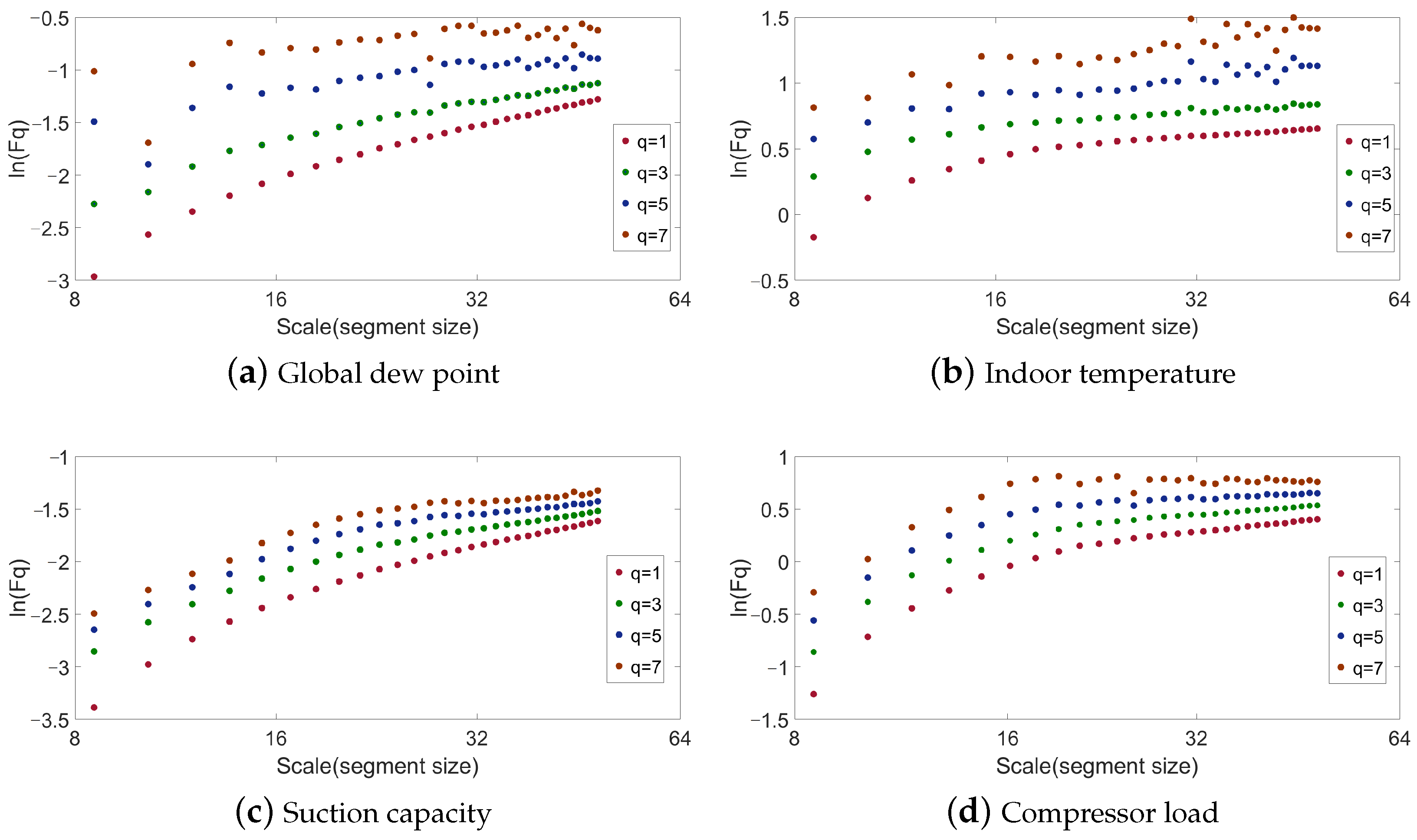
It is noted that F q ( s ) is a function of data length s and fractal order q. As s increases, the function F q ( s ) exhibits an increasing power-law relationship, i.e., F q ( s ) s H q . Here, H q is the Hurst exponent. The power-law relationship of F q ( s ) is usually written as F q ( s ) = A s H q . Taking the logarithmic operation on it, we have
lg F q ( s ) = H q lg s + lg A
where the slope H q is the generalized Hurst exponent. q is the order that affects the fluctuation function F ( v , s ) . It is important to notice that the sequence has a multifractal property when H q changes with fractal order q. On the other hand, the sequence is monofractal when the slope does not change with q. The slope degree determines the size of the fractal; in other words, the fractal characteristic is more obvious when the slope changes sharply.

4. Study Case

The cooling system plays an important role in modern industry and everyday life. Figure 2 shows the structure of the cooling system of a supermarket [5,36]. Initially, the high-pressure liquid water is decompressed and evaporated into gas by the evaporator. Heat is absorbed to freeze goods in the refrigerator. Next, the low pressure gas from the evaporator is pressurized by the compressor. The high pressure gas is then liquefied into liquid water through the condenser machine. The liquid water is again used for evaporation. This whole process consumes a great amount of power and is accompanied by many complex behaviors, which are difficult to model only by traditional analysis methods. This paper takes the energy consumption of a supermarket cooling system as an example to analyze complex systems from the perspective of fractional order thinking. Figure 3 shows the raw data of the global dew point (the temperature at which steam condenses), the indoor temperature, the suction capacity (an index of the compressor), and compressor load, which were collected from March to October.

4.1. Fractional Feature Extraction

Figure 3 shows four raw measurements from the supermarket cooling system, including the global dew point temperature, the indoor temperature, the suction capacity, and the compressor load from 1 March to 31 October 2018. It is clear that they vary dynamically. The compressor load in particular shows a marked increase from June to September. This is obviously the electricity consumed for cooling throughout the summer. The probability density function (PDF) was used to analyze them, as shown in Figure 4. The blue bar displays the histogram distribution, and the red and green lines are the fitting Gaussian distribution and the α -stable distribution, respectively. The α -stable distribution is closer to the real histogram than the Gaussian distribution. The parameters of the α -stable distribution are given in Table 1, in which no α values are equal to 2. Four variables do not obey a Gaussian distribution.
To analyze the variable tendency, Figure 5 shows the autocorrelation function (ACF). The LRD is more obvious if the ACF decays more slowly. The four ACFs all show more or less a decline with the increase in lag. This means that the four variables have a certain LRD feature. According to Table 1, the global dew point temperature has the highest Hurst exponent and the slowest ACF decline. On the contrary, the suction capacity has the smallest Hurst exponent and the biggest ACF decline in initial lag. Its ACF therefore does not change dramatically. Suction capacity is directly related to the cooling temperature. If the cooling temperature is kept constant, the suction capacity of the compressor must remain constant. To guarantee a constant cooling temperature, the compressor load must be increased when the summer is coming.
Once the significant LRD feature was found based on the ACF and the α -stable distribution fitting, the R/S method and the MFDFA method were employed to analyze the hidden fractional features further. Figure 6 shows the corresponding R/S plot, whose slope is the Hurst exponent given in Table 1. The Hurst exponents are all greater than 0.5, indicating that the change trends in the future are the same as they were in the past.
Figure 7 shows the F q function obtained by MFDFA. It shows a different slope under a different order q. This slope is also used to calculate the Hurst exponent. The detailed indices under different scaling are shown in Table 2. MFDFA shows that the four variables have multifractal characteristics and that the Hurst exponents change with a different order q. The global dew point temperature has the highest Δ H , and suction capacity has the lowest Δ H . This indicates that the global dew point temperature is easy to change and that suction capacity is relatively stable. Comparing the raw data in Figure 3, it is found that the result is consistent with the real measurements.

4.2. Energy Prediction Analysis

From the above analysis, the process variables of the cooling system have significant LRD and fractal features, and they do not obey a Gaussian distribution. Therefore, fractional thinking was integrated into the prediction model to predict the energy consumption, which is denoted by the compressor load. The data of April was used for training, and the data of May was employed for testing.
Figure 8 shows the time series after the fractional derivative operation with (a) fractional d = 0.4 and (b) integer d = 1 . The time series after the integer derivative is obviously stationary, and the trend feature is eliminated. On the contrary, the time series after the fractional derivative smooths the original data but retains its trend.
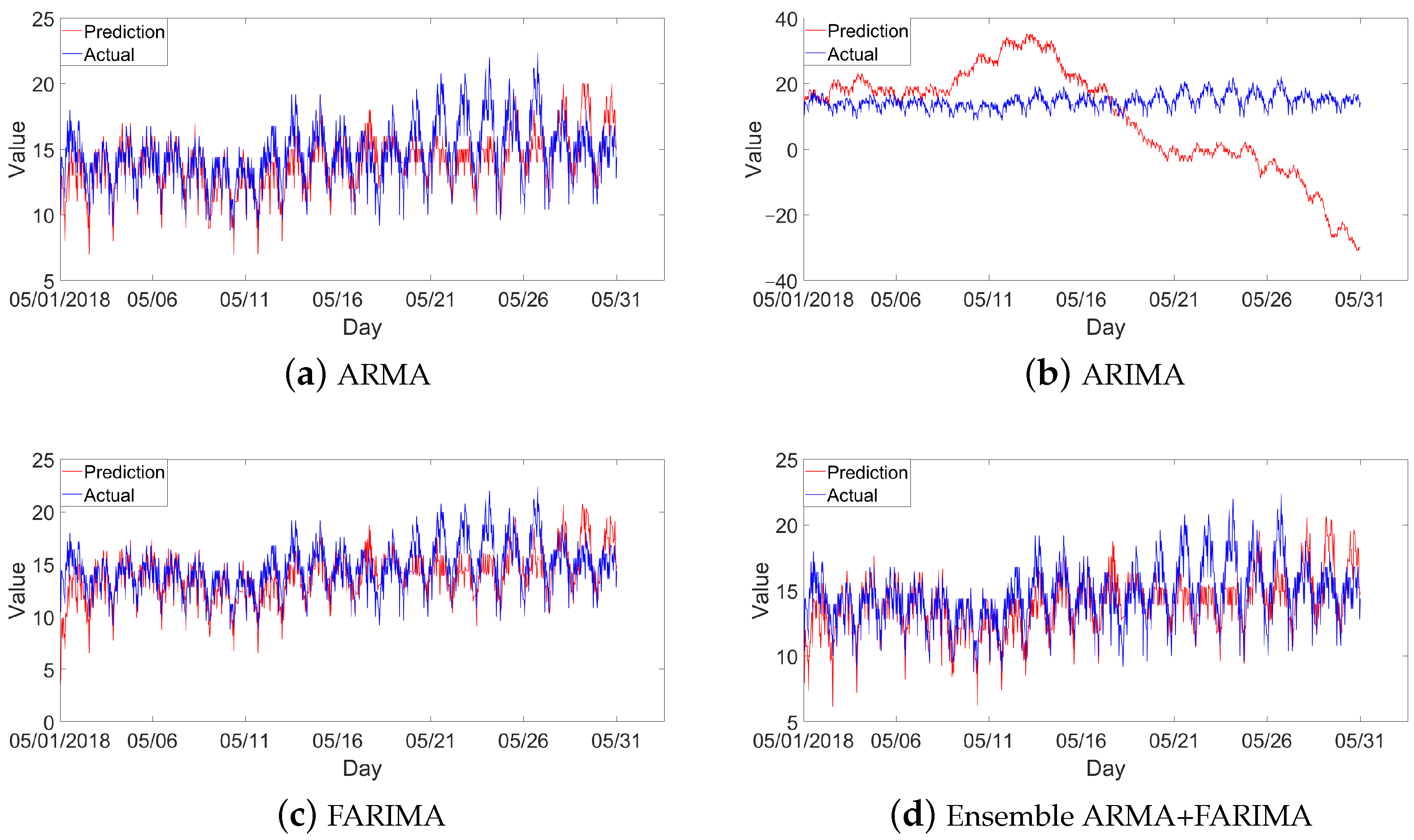
Figure 9 shows the testing results under three different models, ARMA, ARIMA, and FARIMA. The parameters pairs ( d , p , q ) for the three models are ( 0 , 15 , 6 ) , ( 1 , 10 , 10 ) , and ( 0.4 , 15 , 3 ) , respectively. These parameters were obtained by minimizing the root mean square error (RMSE) of the training date. As shown in Figure 9, the prediction value can fit the actual value well in the three models. However, the fitting accuracy of the FARIMA model is significantly higher than the other two models by comparing the root mean square error (RMSE) index, according to Table 3.
Figure 10 shows the testing results of (a) ARMA, (b) ARIMA, and (c) FARIMA. The prediction of the ARIMA model is poorer than the others because the model cannot learn the trend eliminated by the integer delay sampling, as shown in Figure 10. On the contrary, the FARIMA model achieves an accurate prediction result, as shown in Figure 10. An evaluation index comparison for training and testing is given in Table 3, including root mean square error (RMSE) and mean absolute error (MAE). The RMSE and MAE of FARIMA are far smaller than those of ARIMA. Its prediction mean value is very close to the actual mean value of 13.9043. Therefore, considering the training and testing results comprehensively, the FARIMA model simulates the stochastic system when the time series shows typical fractional features.
An ensemble learning strategy was adopted to further improve the accuracy of prediction. Here, ARMA and FARIMA were selected as the basic models because they can well predict energy consumption according to the above analysis. The final prediction is a combination by weight average. Figure 10d is the result of the ensemble model, which achieves a better performance when predicting the actual energy consumption in May. The accuracy of the ensemble model is higher than that of the other three single models.

5. Conclusions

This paper presents fractional analytics for a time series in a real industrial system. Several fractional features, such as the LRD, self-similiarity, and the multifractal property, are analyzed using the Hurst exponent and fractal theory. An ensemble FARIMA model is then proposed to predict the energy consumption of a supermarket cooling system. Variables, including the suction capacity, the indoor temperature, the global dew point temperature, and the compressor load, were selected to find the trend and LRD features. Based on the PDF fitting results, an α -stable distribution is a better representation than a Gaussian distribution. All Hurst exponents are higher than 0.5, and the MFDFA methods also indicate a significant fractional feature. The prediction results of the three regression models, ARMA, ARIMA, and FARIMA, were evaluated. The FARIMA model performs well for a time series with typical fractional behavior. For a complex industrial process, fractional analytics is effective in mining the useful information hidden in the process variables.

Author Contributions

These authors contributed equally to this work. Conceptualization, methodology, validation, J.W., H.W., S.L. and M.Z.; formal analysis, M.Z.; investigation, J.W., S.L. and M.Z.; resources, data curation, J.W. and H.W.; writing—original draft preparation, Y.L. and J.W.; writing—review and editing, J.W., H.W., S.L. and M.Z.; software, visualization, Y.L. and H.W.; supervision, J.W. and S.L.; project administration, J.W. and S.L.; funding acquisition, J.W. and S.L. All authors have read and agreed to the published version of the manuscript.

Funding

This research is funded by the National Natural Science Foundation of China (61973023, 62003220), Beijing Natural Science Foundation (4202052) and Innovation Team by Department of Education of Guangdong Province, China (2020KCXTD041).

Institutional Review Board Statement

Not applicable.

Informed Consent Statement

Not applicable.

Data Availability Statement

Not applicable.

Conflicts of Interest

The authors declare no conflict of interest.

References

  1. Albada, V.S.J.; Robinson, P.A. Transformation of arbitrary distributions to the normal distribution with application to eeg test-retest reliability. J. Neurosci. Methods 2018, 161, 205–211. [Google Scholar] [CrossRef] [PubMed] [Green Version]
  2. Sakia, R.M. The Box-Cox transformation technique: A review. Statistician 1992, 41, 169–178. [Google Scholar] [CrossRef]
  3. Zhang, X.F.; Chen, Y.Q. Admissibility and robust stabilization of continuous linear singular fractional order systems with the fractional order α: The 0 < α < 1 case. ISA Trans. 2018, 82, 42–50. [Google Scholar] [PubMed]
  4. Andrews, B.; Calder, M.; Davis, R.A. Maximum likelihood estimation for α-stable autoregressive processes. Ann. Stat. 2009, 37, 1946–1982. [Google Scholar] [CrossRef]
  5. Wang, J.; Wang, J.Q.; Chen, Y.Q.; Zhang, Y.Z. Fractional Stochastic Configuration Networks-Based Nonstationary Time Series Prediction and Confidence Interval Estimation. Expert Syst. Appl. 2022, 192, 116357. [Google Scholar] [CrossRef]
  6. Li, X.; Wang, S.; Fan, L. Mixture approximation to the amplitude statistics of isotropic α-stable clutter. Signal Process. 2014, 99, 86–91. [Google Scholar] [CrossRef]
  7. Diego, S.G.; Ercan, E.K.; Diego, P.R. Modelling and Assessing Differential Gene Expression Using the Alpha Stable Distribution. Int. J. Biostat. 2009, 5, 16. [Google Scholar]
  8. Zhang, X.F.; Huang, W.K. Adaptive neural network sliding mode control for nonlinear singular fractional order systems with mismatched uncertainties. Fractal Fract. 2020, 4, 50. [Google Scholar] [CrossRef]
  9. Zhang, J.X.; Yang, G.H. Fault-tolerant output-constrained control of unknown Euler-Lagrange systems with prescribed tracking accuracy. Automatica 2020, 111, 108606. [Google Scholar] [CrossRef]
  10. Zhang, J.X.; Yang, G.H. Fuzzy adaptive output feedback control of uncertain nonlinear systems with prescribed performance. IEEE Trans. Cybern. 2018, 48, 1342–1354. [Google Scholar] [CrossRef]
  11. Wang, J.; Shao, C.F.; Chen, Y.Q. Fractional order sliding mode control via disturbance observer for a class of fractional order systems with mismatched disturbance. Mechatronics 2018, 53, 8–19. [Google Scholar] [CrossRef]
  12. Zhang, X.; Liu, R.; Ren, J.; Gui, Q. Adaptive Fractional Image Enhancement Algorithm Based on Rough Set and Particle Swarm Optimization. Fractal Fract. 2022, 6, 100. [Google Scholar] [CrossRef]
  13. Zhang, X.; Dai, L. Image Enhancement Based on Rough Set and Fractional Order Differentiator. Fractal Fract. 2022, 6, 214. [Google Scholar] [CrossRef]
  14. Yan, H.; Zhang, J.; Zhang, X. Injected Infrared and Visible Image Fusion via L1 Decomposition Model and Guided Filtering. IEEE Trans. Comput. Imaging 2022, 8, 162–173. [Google Scholar] [CrossRef]
  15. Liu, Y.; Zhang, Y.H.; Qiu, T.S. Improved time difference of arrival estimation algorithms for cyclostationary signals in α-stable impulsive noise. Digit. Signal Process. 2018, 76, 94–105. [Google Scholar] [CrossRef]
  16. Ihlen, A.; Espen, F. The influence of power law distributions on long-range trial dependency of response times. J. Math. Psychol. 2013, 57, 215–224. [Google Scholar] [CrossRef]
  17. Clauset, A.; Shalizi, C.R.; Newman, M.E.J. Power-law distributions in empirical data. Siam Rev. 2009, 51, 661–703. [Google Scholar] [CrossRef] [Green Version]
  18. Lel, W.E.; Taqqu, M.S.; Willinger, W. On the self-similar nature of ethernet traffic. Acm Sigcomm Comput. Commun. Rev. 1995, 25, 202–213. [Google Scholar]
  19. Kourtsoyiannis, D.; Climate, C. The Hurst phenomenon and hydrological statistics. Int. Assoc. Sci. Hydrol. Bull. 2003, 48, 3–24. [Google Scholar] [CrossRef]
  20. Bregni, S.; Primerano, L. Using the modified allan variance for accurate estimation of the hurst parameter of long-range dependent traffic. IEEE Trans. Commun. 2008, 56, 1900–1906. [Google Scholar] [CrossRef]
  21. Grech, D.; Pamua, G. The local Hurst exponent of the financial time series in the vicinity of crashes on the Polish stock exchange market. Phys. A Stat. Mech. Its Appl. 2008, 387, 4299–4308. [Google Scholar] [CrossRef]
  22. Tyralis, H.; Dimitriadis, P.; Koutsoyiannis, D. On the long-range dependence properties of annual precipitation using a global network of instrumental measurements. Adv. Water Resour. 2018, 111, 301–318. [Google Scholar] [CrossRef]
  23. Pandit, P.; Ardakan, M.S.; Amini, A.A. High-dimensional bernoulli autoregressive process with long range dependence. arXiv 2019, arXiv:1903.09631. [Google Scholar]
  24. Chen, Y.; Ye, X.; Zhang, J. Effects of trends and seasonalities on robustness of the Hurst parameter estimators. IET Signal Process. 2012, 6, 849–856. [Google Scholar]
  25. Pianese, A.; Bianchi, S. Fast and unbiased estimator of the time-dependent Hurst exponent. Chaos 2018, 28, 031102. [Google Scholar] [CrossRef]
  26. Karp, A.; Vuuren, G.V. Investment implications of the fractal market hypothesis. Ann. Financ. Econ. 2019, 14, 1950001. [Google Scholar] [CrossRef]
  27. Yu, Q.Y.; Dai, Z.X. Estimation of sandstone permeability with sem images based on fractal theory. Transp. Porous Media 2019, 126, 701–712. [Google Scholar] [CrossRef]
  28. Hu, K.; Ivanov, P.C.; Chen, Z. Effect of trends on detrended fluctuation analysis. Phys. Rev. E Stat. Nonlin Soft Matter Phys. 2001, 64, 011114. [Google Scholar] [CrossRef] [Green Version]
  29. Chen, Z.; Ivanov, P. Effect of nonstationarities on detrended fluctuation analysis. Phys. Rev. E Stat. Nonlin Soft Matter Phys. 2002, 65, 041107. [Google Scholar] [CrossRef] [Green Version]
  30. Kantelhardt, J.W.; Zschiegner, S.A. Multifractal detrended uctuation analysis of nonstationary time series. Phys. A Stat. Mech. Appl. 2002, 316, 87–114. [Google Scholar] [CrossRef] [Green Version]
  31. Zhu, H.; Zhang, W. Multifractal property of Chinese stock market in the CSI 800 index based on MF-DFA approach. Phys. A Stat. Mech. Appl. 2018, 490, 497–503. [Google Scholar] [CrossRef]
  32. Hillmer, S.C.; Tiao, G.C. An ARIMA-model-based approach to seasonal adjustment. Publ. Am. Stat. Assoc. 1982, 77, 63–70. [Google Scholar] [CrossRef]
  33. Hedrea, E.L.; Precup, R.E.; Roman, R.C.; Petriu, E.M. Tensor product-based model transformation approach to tower crane systems modeling. Asian J. Control. 2021, 23, 1313–1323. [Google Scholar] [CrossRef]
  34. Kataria, A.; Ghosh, S.; Karar, V. Data Prediction of Electromagnetic Head Tracking using Self Healing Neural Model for Head-Mounted Display. Rom. J. Inf. Sci. Technol. 2020, 23, 354–367. [Google Scholar]
  35. Greff, K.; Srivastava, R.K.; Koutnik, J. LSTM: A search space odyssey. IEEE Trans. Neural Netw. Learn. Syst. 2016, 28, 2222–2232. [Google Scholar] [CrossRef] [PubMed] [Green Version]
  36. Wang, J.Q.; Du, Y.; Wang, J. Lstm based long-termenergy consumption prediction with periodicity. Energy 2021, 197, 117197. [Google Scholar] [CrossRef]
  37. Scardapane, S.; Wang, D.H. Randomness in neural networks: An overview. Wiley Interdiscip. Rev. Data Min. Knowl. Discov. 2017, 7, 1–8. [Google Scholar] [CrossRef]
  38. Zhang, X. Relationship between integer order systems and fractional order system and its two applications. IEEE/CAA J. Autom. Sin. 2018, 5, 639–643. [Google Scholar] [CrossRef]
  39. Kun, H.; Jun, W. A botnet detection method based on FARIMA and hill-climbing algorithm. Int. J. Mod. Phys. B. 2019, 32, 1850356. [Google Scholar] [CrossRef]
  40. Sheng, H.; Chen, Y.Q. FARIMA with stable innovations model of great salt lake elevation time series. Signal Process. 2011, 91, 553–561. [Google Scholar] [CrossRef]
  41. Suhail, Y.; Upadhyay, M.; Chhibber, A. Machine Learning for the Diagnosis of Orthodontic Extractions: A Computational Analysis Using Ensemble Learning. Bioengineering 2020, 7, 55. [Google Scholar] [CrossRef] [PubMed]
  42. Xiao, Q.Y.; Chang, H.H.; Geng, G.; Yang, L.Y. An ensemble machine-learning model to predict historical PM2.5 concentrations in China from satellite data. Environ. Sci. Technol. 2018, 52, 13260–13269. [Google Scholar] [CrossRef] [PubMed]
  43. Ortigueira, M.D.; Magin, R.L. On the Equivalence between Integer- and Fractional Order-Models of Continuous-Time and Discrete-Time ARMA Systems. Fractal Fract. 2022, 6, 242. [Google Scholar] [CrossRef]
  44. Ortigueira, M.D.; Coito, F.J.V.; Trujillo, J.J. Discrete-time differential systems. Signal Process. 2015, 107, 198–217. [Google Scholar] [CrossRef]
  45. Granger, C.W.J.; Joyeux, R. An introduction to long-memory time series and fractional differencing. J. Time Ser. Anal. 1980, 1, 15–30. [Google Scholar] [CrossRef]
  46. Mikosch, T.; Gadrich, T.; Kluppelberg, C.; Adler, R.J. Parameter estimation for ARMA models with inifite variance innovations. Ann. Stat. 1995, 23, 305–326. [Google Scholar] [CrossRef]
  47. Kokoszka, P.S.; Taqqu, M.S. Fractional ARIMA with stable innovations. Stoch. Process. Their Appl. 1995, 60, 19–47. [Google Scholar] [CrossRef] [Green Version]
  48. Zheng, T.; Chen, R. Dirichlet ARMA models for compositional time series. J. Multivar. Anal. 2017, 158, 31–46. [Google Scholar] [CrossRef] [Green Version]
  49. Salasgonzalez, D.; Gorriz, J.M.; Ramirez, J. Parameterization of the distribution of white and grey matter in MRI using the α-stable distribution. Comput. Biol. Med. 2013, 43, 559–567. [Google Scholar] [CrossRef]
  50. Althoff, M.; Stursberg, O.; Buss, M. Estimating the parameters of an α-stable distribution using the existence of moments of order statistics. Stat. Probab. Lett. 2014, 90, 78–84. [Google Scholar]
  51. Tierra, A.; Luna, M.; Staller, A. Hurst coefficient estimation by rescaled range and wavelet of the ENU Coordinates time series in GNSS network. IEEE Lat. Am. Trans. 2018, 16, 1064–1069. [Google Scholar] [CrossRef]
  52. Moulines, E.; Roueff, F.; Taqqu, M.S. A wavelet whittle estimator of the memory parameter of a nonstationary Gaussian time series. Ann. Stat. 2008, 36, 1925–1956. [Google Scholar] [CrossRef]
  53. Leonardo, R.G.; Galib, H.; Jurgen, K.; Dirk, W. MFDFA: Efficient multifractal detrended fluctuation analysis in python. Comput. Phys. Commun. 2022, 273, 108254. [Google Scholar]
  54. Ihlen, E.A.F. Introduction to multifractal detrended fluctuation analysis in Matlab. Front. Physiol. 2021, 3, 141. [Google Scholar] [CrossRef] [Green Version]
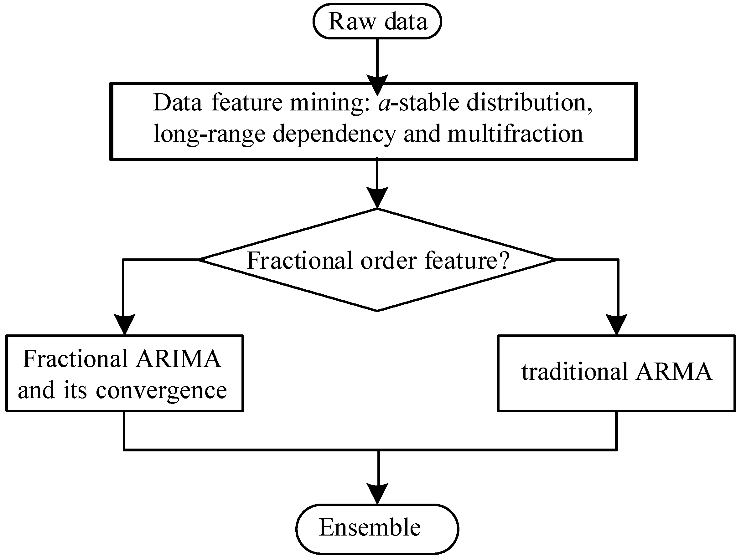
Figure 1. Industrial data analytics procedure.
Fractalfract 06 00276 g001
Figure 2. The structure of a supermarket cooling system.
Fractalfract 06 00276 g002
Figure 3. Raw measurments of four key variables.
Fractalfract 06 00276 g003
Figure 4. PDF fitting of the raw data.
Fractalfract 06 00276 g004
Figure 5. ACF of the variables.
Fractalfract 06 00276 g005
Figure 6. R/S plot.
Figure 6. R/S plot.
Fractalfract 06 00276 g006
Figure 7. Scaling function Fq.
Fractalfract 06 00276 g007
Figure 8. Time series after the fractional derivative operation.
Fractalfract 06 00276 g008
Figure 9. Training result comparison.
Fractalfract 06 00276 g009
Figure 10. Testing result comparison.
Fractalfract 06 00276 g010
Table 1. Parameters of the α -stable distribution and the Hurst exponent.
Variable α β γ δ Hurst
Global dew point temp.1.684512.157256.05840.9199
Indoor temperature1.7927−10.718572.53500.9342
Suction capacity1.49500.11961.082150.70360.8126
Compressor load1.979811.706016.32460.9798
Table 2. Indices obtained by the MFDFA method.
Variable q = 1 q = 3 q = 5 q = 7 Δ H
Global dew point temp.0.68960.50210.32710.25990.4297
Indoor temperature0.72650.55820.50440.47410.2524
Suction capacity0.27910.19130.22980.26970.0878
Compressor load0.59020.47830.39700.32080.2694
Table 3. Model performance evaluation.
TrainingTesting
ModelRMSEMAERMSEMax ErrorPredict Mean
ARMA1.10351.56132.02447.600014.6497
ARIMA2.094213.796217.313124.60009.9240
FARIMA0.35911.54972.03728.000014.6479
ARMA + FARIMA1.53011.99807.800014.6488
Publisher’s Note: MDPI stays neutral with regard to jurisdictional claims in published maps and institutional affiliations.