The Construction of High-Order Robust Theta Methods with Applications in Subdiffusion Models

Abstract

An exponential-type function was discovered to transform known difference formulas by involving a shifted parameter $\theta$ to approximate fractional calculus operators. In contrast to the known $\theta$ methods obtained by polynomial-type transformations, our exponential-type $\theta$ methods take the advantage of the fact that they have no restrictions in theory on the range of $\theta$ such that the resultant scheme is asymptotically stable. As an application to investigate the subdiffusion problem, the second-order fractional backward difference formula is transformed, and correction terms are designed to maintain the optimal second-order accuracy in time. The obtained exponential-type scheme is robust in that it is accurate even for very small $\alpha$ and can naturally resolve the initial singularity provided $\theta =-\frac{1}{2}$, both of which are demonstrated rigorously. All theoretical results are confirmed by extensive numerical tests.

1. Introduction

Diffusion is one of the most common phenomena of the physical world in which a particle’s motion is Brownian and can be characterized by the classical model ${\partial }_{t}u-\Delta u=f$. It is well known that Brownian motions assume that mean-squared particle displacements grow linearly with respect to time t, whereas an increasing list of experiments in the last decades indicates that such growths can be sublinear or superlinear; i.e., the diffusion can be anomalous. From a macro-perspective, the probability density function u in anomalous diffusion obeys the equation involving a fractional order derivative [1,2]. In this work, we concern ourselves with the subdiffusion transport mechanism (with the fractional derivative order $\alpha \in (0,1)$), which has received much attention in recent years, since the electron transport, thermal diffusion, and protein transport, among others, reveal that the underlying stochastic process is the continuous time random walk instead of Brownian motions [1,2,3,4]. Perhaps the simplest subdiffusion model [2,5] takes the following form:

$${\partial }_t^{\alpha }u(\mathbf{x},t)-\Delta u(\mathbf{x},t)=f(\mathbf{x},t),$$

(1)

with suitable initial boundary conditions. Here, ${\partial }_t^{\alpha }$ denotes the Caputo fractional operator [6] of order $\alpha \in (0,1)$:

$$\left({\partial }_t^{\alpha }\varphi \right)\left(t\right)=\frac{1}{\mathrm{\Gamma }(1-\alpha )}{\int }_0^t\frac{{\varphi }^{\prime }\left(s\right)}{{(t-s)}^{\alpha }}\mathrm{d}s,$$

which satisfies ${\partial }_t^{\alpha }\varphi =D_t^{\alpha }(\varphi -\varphi \left(0\right))$ where $D_t^{\alpha }$ is the Riemann–Louisville fractional differential operator [6].

$$\left(D_t^{\alpha }\varphi \right)\left(t\right)=\frac{1}{\mathrm{\Gamma }(1-\alpha )}\frac{\mathrm{d}}{\mathrm{d}t}{\int }_0^t\frac{\varphi \left(s\right)}{{(t-s)}^{\alpha }}\mathrm{d}s.$$

Its integral counterpart, the Riemann-Liouville fractional integral operator [6] $D_t^{-\alpha }\varphi$ is defined by

$$\left(D_t^{-\alpha }\varphi \right)\left(t\right)=\frac{1}{\mathrm{\Gamma }\left(\alpha \right)}{\int }_0^t\frac{\varphi \left(s\right)}{{(t-s)}^{1-\alpha }}\mathrm{d}s.$$

The literature on numerically exploring the fractional calculus operators is vast. The authors of [7,8] proposed the well-known L1 method for the Caputo fractional derivative, which is convergent of order $2-\alpha$. Lubich [9] systematically developed the convolution quadrature (CQ) theory for discretizing the operators $D_t^{\alpha }$ and $D_t^{-\alpha }$. The well-known fractional linear multistep methods, which include the Grünwald formula [6] and pth-order fractional backward difference formulas (BDF-p) as special cases, belong to such framework. Some other difference formulas that essentially fit the framework of convolution quadrature can be found in [10,11,12], to mention just a few. In [13], the authors developed the shifted Grünwald formula to overcome the instability of the Grünwald formula when applied to fractional advection–dispersion flow equations. Galeone and Garrappa [14] devised explicit multistep methods for the fractional derivative and examined the stability properties in much detail. By weighting and averaging the shifted Grünwald formula, Tian et al. [15] proposed the weighted and shifted Grünwald difference formulas for space fractional Riemann–Louisville derivatives. Ding et al. [16] built a second-order midpoint formula by shifting the fractional BDF-2 and applied it to fractional cable equations. In [17], the authors investigated shifted convolution quadrature (SCQ) methods in detail aiming to develop $\theta$-methods systematically, where a polynomial-type transformation strategy was proposed to convert any known CQ method into a $\theta$ method. However, the existence of zeros of polynomials severely restricts the choice of the parameter $\theta$ such that the method is A-stable. In this work, we propose a novel transformation strategy by resorting to the exponential-type function, illustrating its superiority in developing A-stable methods and robust numerical schemes for subdiffusion problems.

Clearly, the fractional operators mentioned above involve a weak singular kernel $s^{-\gamma }$ for some $\gamma \in (0,1)$, which renders numerically solving subdiffusion problems rather difficult, since most high-order difference formulas, if directly applied to such problem on uniform meshes, lose their deserved high accuracy [18,19,20]. To resolve such difficulties, modified difference formulas by adding correction terms [21,22,23,24,25] or using nonuniform meshes are developed [26,27], to mention just a few. Specifically, Yan et al. [21] developed the modified L1 method by adding correction terms to recover the optimal convergence order $2-\alpha$, while Jin et al. [22] established the corrected fractional BDF-p to restore the high accuracy. By shifting the approximation point by $\frac{\alpha }{2}$ with respect to grid points, Jin et al. [23] designed a two-step correction method for the fractional Crank–Nicolson scheme and such a correction technique was further optimized by Wang et al. [24] where only the first-step correction is needed to maintain the optimal accuracy. In particular, we studied a general second-order difference scheme for (1) in [25], which is generated by an SCQ difference formula with a free parameter $\theta \in (0,\frac{1}{2})$ and can preserve the high accuracy if correction terms are added. The $\theta =\frac{1}{2}$ is excluded there for the singularity of the corresponding transform functions involved in theoretical analysis. Indeed, the case $\theta =\frac{1}{2}$ is of special interest since the correction terms vanish, enlightening us that a carefully designed time-stepping method, even on uniform meshes, should automatically resolve the singularity. A close examination, as shown in this study, indicates that the singularity of transform functions stems from the zeros of polynomials, which can be avoided by using the exponential-type transform functions. To sum up, the contribution of this study comes from three aspects:

• An exponential-type transformation strategy is proposed to transfer any known pth order ($p\le 6$) time-stepping methods into $\theta$ methods with the same accuracy.
• The robustness of numerical schemes obtained by the exponential-type transformation strategy for a trial equation is examined theoretically and verified numerically.
• Rigorous arguments of the optimal error estimates of the transformed fractional BDF-2 are provided for the subdiffusion Problem (1).

The rest of the article is outlined as follows. In Section 2, we first review some basic aspects of the SCQ and then determine the stability region of $\theta$ methods when applied to a simple differential equation. In Section 3, we propose the exponential-type transformation to convert known stepping methods into $\theta$ methods and demonstrate its superiority over traditional polynomial-type transformations. In Section 4, the exponentially transformed fractional BDF-2 is applied to subdiffusion problems where correction terms are designed to recover the optimal convergence rate, which are confirmed rigorously by theoretical analyses. Extensive numerical tests are offered in Section 5 to verify all theoretical results. Finally, in Section 6, we make some concluding remarks.

2. Preliminaries

2.1. Review of $\theta$-Methods in SCQ

The construction of novel robust $\theta$ methods is based on the framework of shifted convolution quadrature [28] for the fractional calculus, which will be introduced briefly in this subsection.

Divide the time interval $[0,T]$ by the following grids: $0=t_0<t_1<\cdots <t_N=T$ with $t_n=n\tau$ and $\tau =T/N$. Let ${\varphi }^n$ be the value of a function $\varphi \left(t_n\right)$ for the sake of simplicity. Given a sequence ${\left\{{\omega }_j\right\}}_{j=0}^{\infty }$, the difference formula

$$D_{\tau ,\theta }^{\alpha ,n}\varphi :={\tau }^{-\alpha }\sum _{j=0}^n{\omega }_j{\varphi }^{n-j}$$

(2)

represents an approximation to the Riemann–Louisville derivative $\left(D_t^{\alpha }\varphi \right)\left(t_{n-\theta }\right)$ if the generating function $\omega \left(\zeta \right)$ defined by $\omega \left(\zeta \right)={\sum }_{j=0}^{\infty }{\omega }_j{\zeta }^j$ for $\left|\zeta \right|<1$ satisfies

$$\left(\mathrm{i}\right)\mathrm{Stability}:{\omega }_n=O\left(n^{-\alpha -1}\right),\left(\mathrm{ii}\right)\mathrm{Consistency}:{\tau }^{-\alpha }{e}^{\theta \tau }\omega \left(e^{-\tau }\right)-1=o\left(1\right),$$

(3)

simultaneously.

Lemma 1

(See [28], Theorem 1). The difference Formula (2) is pth-order convergent if and only if both the stability in (3) and the following consistent condition

$$\mathit{Consistency}\mathit{of}\mathit{order}p:{\tau }^{-\alpha }{e}^{\theta \tau }\omega \left(e^{-\tau }\right)-1=O\left({\tau }^p\right)$$

(4)

are fulfilled.

It is notable that if the shift parameter $\theta$ vanishes in (2) or (4), meaning that a difference formula $D_{\tau }^{\alpha ,n}\varphi :=D_{\tau ,0}^{\alpha ,n}\varphi$ is designed for $D_t^{\alpha }\varphi$ at the grid point $t_n$; then, one essentially obtains approximation methods belonging to the convolution quadrature theory, which was partially founded in [9] for approximating fractional calculus and then extended to more general convolution-type operators [29,30]. In previous studies, we have extended several traditional difference formulas such as the fractional BDF-2 [31], the fractional trapezoidal rule [17], and the fractional Adams–Moulton method [32], among others, to their generalized versions by involving shifted parameter $\theta$. Moreover, a conversion strategy was proposed in [28] to transform a difference formula $D_{\tau }^{\alpha ,n}\varphi$ into $D_{\tau ,\theta }^{\alpha ,n}\varphi$, which, in the viewpoint of the generating function reconstruction, can be stated as follows:

$$\omega \left(\zeta \right)={\varpi }_p\left(\zeta \right)\Theta (\zeta ;\theta ),\Theta (\zeta ;\theta )={\gamma }_0+{\gamma }_1(1-\zeta )+{\gamma }_2{(1-\zeta )}^2+\cdots +{\gamma }_{p-1}{(1-\zeta )}^{p-1},$$

(5)

where ${\varpi }_p\left(\zeta \right)={\sum }_{j=0}^{\infty }{\varpi }_j{\zeta }^j$ represents the generating function with ${\varpi }_j$ from the weights of $D_{\tau }^{\alpha ,n}\varphi$, which is convergent of order p. The ${\gamma }_j$ s are obtained from identity ${\sum }_{i=0}^{\infty }{\gamma }_i{(1-\zeta )}^i={\zeta }^{\theta }$. Specifically, the second-, third- and fourth-order transformed generating functions take the following forms:

$$\omega \left(\zeta \right)=\left\{\begin{array}{cc}{\varpi }_2\left(\zeta \right)\left[(1-\theta )+\theta \zeta \right],\hfill & \mathrm{f}\mathrm{o}\mathrm{r}\mathrm{2}\mathrm{n}\mathrm{d}\text{-}\mathrm{o}\mathrm{r}\mathrm{d}\mathrm{e}\mathrm{r},\hfill \\ {\varpi }_3\left(\zeta \right)\left[\frac{1}{2}(1-\theta )(2-\theta )+\theta (2-\theta )\zeta +\frac{1}{2}\theta (\theta -1){\zeta }^2\right],\hfill & \mathrm{f}\mathrm{o}\mathrm{r}\mathrm{3}\mathrm{r}\mathrm{d}\text{-}\mathrm{o}\mathrm{r}\mathrm{d}\mathrm{e}\mathrm{r},\hfill \\ {\varpi }_4\left(\zeta \right)[\frac{1}{6}(1-\theta )(2-\theta )(3-\theta )+\frac{1}{2}\theta (2-\theta )(3-\theta )\zeta \hfill \\ -\frac{1}{2}\theta (1-\theta )(3-\theta ){\zeta }^2+\frac{1}{6}\theta (1-\theta )(2-\theta ){\zeta }^3],\hfill & \mathrm{f}\mathrm{o}\mathrm{r}\mathrm{4}\mathrm{t}\mathrm{h}\text{-}\mathrm{o}\mathrm{r}\mathrm{d}\mathrm{e}\mathrm{r},\hfill \end{array}\right.$$

(6)

where ${\varpi }_p\left(\zeta \right)(p=2,3)$ stands for any generating functions in CQ that is convergent of order p.

$$\begin{array}{cc}\hfill {\varpi }_2\left(\zeta \right)& =\left\{\begin{array}{cc}{\left(\frac{3}{2}-2\zeta +\frac{1}{2}{\zeta }^2\right)}^{\alpha },\hfill & \mathrm{f}\mathrm{r}\mathrm{a}\mathrm{c}\mathrm{t}\mathrm{i}\mathrm{o}\mathrm{n}\mathrm{a}\mathrm{l}\mathrm{B}\mathrm{D}\mathrm{F}\text{-}\mathrm{2},\hfill \\ {(1-\zeta )}^{\alpha }\left[1+\frac{\alpha }{2}(1-\zeta )\right],\hfill & \mathrm{2}\mathrm{n}\mathrm{d}\text{-}\mathrm{o}\mathrm{r}\mathrm{d}\mathrm{e}\mathrm{r}\mathrm{N}\mathrm{e}\mathrm{w}\mathrm{t}\mathrm{o}\mathrm{n}\text{-}\mathrm{G}\mathrm{r}\mathrm{e}\mathrm{g}\mathrm{o}\mathrm{r}\mathrm{y}\mathrm{f}\mathrm{o}\mathrm{r}\mathrm{m}\mathrm{u}\mathrm{l}\mathrm{a},\hfill \end{array}\right.\hfill \\ \hfill {\varpi }_3\left(\zeta \right)& =\left\{\begin{array}{cc}{\left(\frac{11}{6}-3\zeta +\frac{3}{2}{\zeta }^2-\frac{1}{3}{\zeta }^3\right)}^{\alpha },\hfill & \mathrm{f}\mathrm{r}\mathrm{a}\mathrm{c}\mathrm{t}\mathrm{i}\mathrm{o}\mathrm{n}\mathrm{a}\mathrm{l}\mathrm{B}\mathrm{D}\mathrm{F}\text{-}\mathrm{3},\hfill \\ {(1-\zeta )}^{\alpha }[1+\frac{\alpha }{2}(1-\zeta )\hfill \\ +(\frac{1}{8}{\alpha }^2+\frac{5\alpha }{24}){(1-\zeta )}^2],\hfill & \mathrm{3}\mathrm{r}\mathrm{d}\text{-}\mathrm{o}\mathrm{r}\mathrm{d}\mathrm{e}\mathrm{r}\mathrm{N}\mathrm{e}\mathrm{w}\mathrm{t}\mathrm{o}\mathrm{n}\text{-}\mathrm{G}\mathrm{r}\mathrm{e}\mathrm{g}\mathrm{o}\mathrm{r}\mathrm{y}\mathrm{f}\mathrm{o}\mathrm{r}\mathrm{m}\mathrm{u}\mathrm{l}\mathrm{a},\hfill \end{array}\right.\hfill \\ \hfill {\varpi }_4\left(\zeta \right)& =\left\{\begin{array}{cc}{\left(\frac{25}{12}-4\zeta +3{\zeta }^2-\frac{4}{3}{\zeta }^3+\frac{1}{4}{\zeta }^4\right)}^{\alpha },\hfill & \mathrm{f}\mathrm{r}\mathrm{a}\mathrm{c}\mathrm{t}\mathrm{i}\mathrm{o}\mathrm{n}\mathrm{a}\mathrm{l}\mathrm{B}\mathrm{D}\mathrm{F}\text{-}\mathrm{4},\hfill \\ {(1-\zeta )}^{\alpha }[1+\frac{\alpha }{2}(1-\zeta )\hfill \\ +(\frac{1}{8}{\alpha }^2+\frac{5\alpha }{24}){(1-\zeta )}^2\hfill \\ +(\frac{1}{48}{\alpha }^3+\frac{5{\alpha }^2}{48}+\frac{\alpha }{8}){(1-\zeta )}^3],\hfill & \mathrm{4}\mathrm{t}\mathrm{h}\text{-}\mathrm{o}\mathrm{r}\mathrm{d}\mathrm{e}\mathrm{r}\mathrm{N}\mathrm{e}\mathrm{w}\mathrm{t}\mathrm{o}\mathrm{n}\text{-}\mathrm{G}\mathrm{r}\mathrm{e}\mathrm{g}\mathrm{o}\mathrm{r}\mathrm{y}\mathrm{f}\mathrm{o}\mathrm{r}\mathrm{m}\mathrm{u}\mathrm{l}\mathrm{a}.\hfill \end{array}\right.\hfill \end{array}$$

(7)

We also mention that transformation (5) indicates that the function $\varphi \left(t\right)=D_t^0\varphi$ at time $t_{n-\theta }$ can be approximated, in accordance with (2), by formula ${\sum }_{j=0}^n{\theta }_j{\varphi }^{n-j}$ with the weights ${\left\{{\theta }_j\right\}}_{j=0}^{\infty }$ generated by $\Theta (\zeta ;\theta )$, where identity ${\varpi }_p\left(\zeta \right)\equiv 1$ is prescribed.

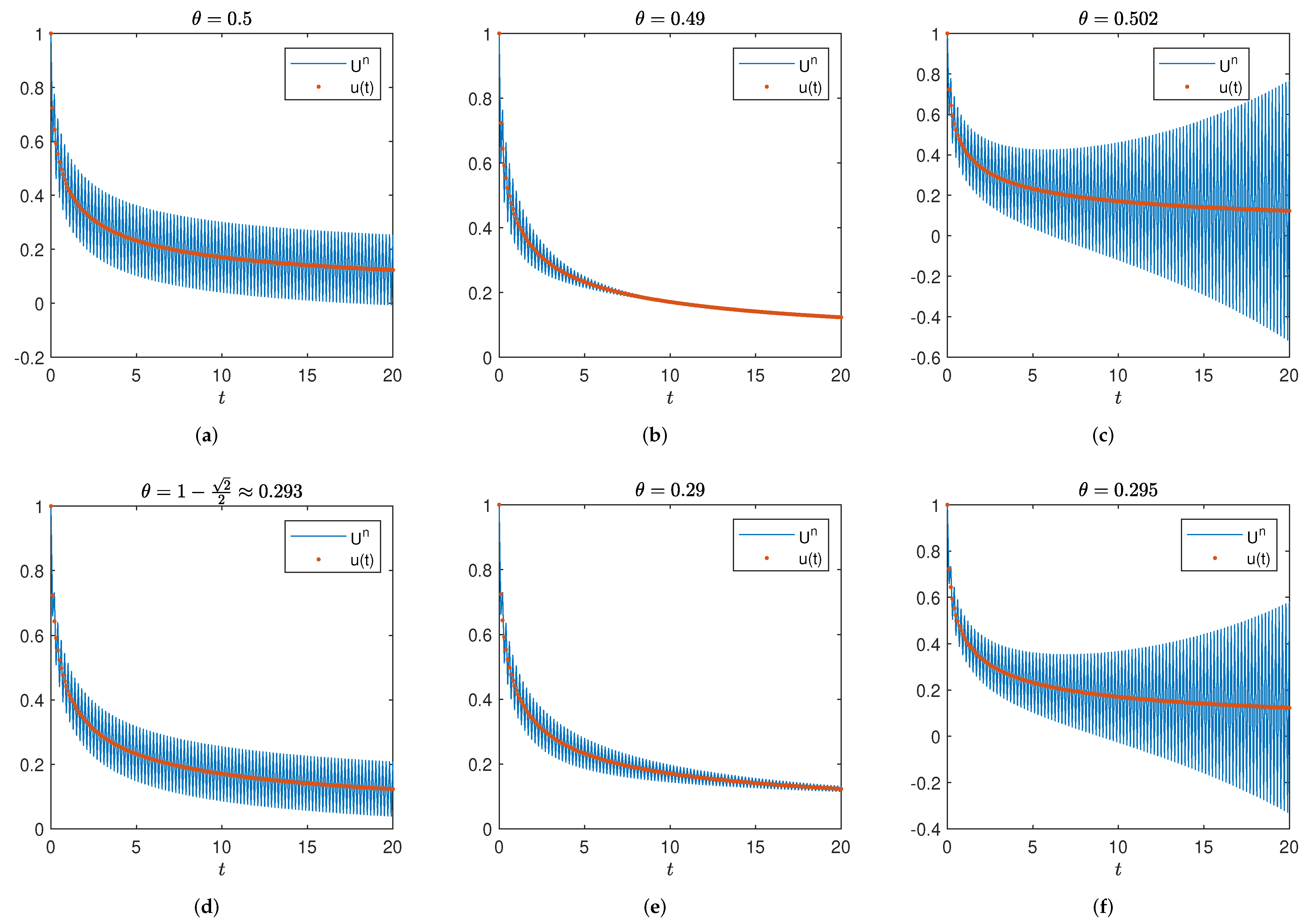
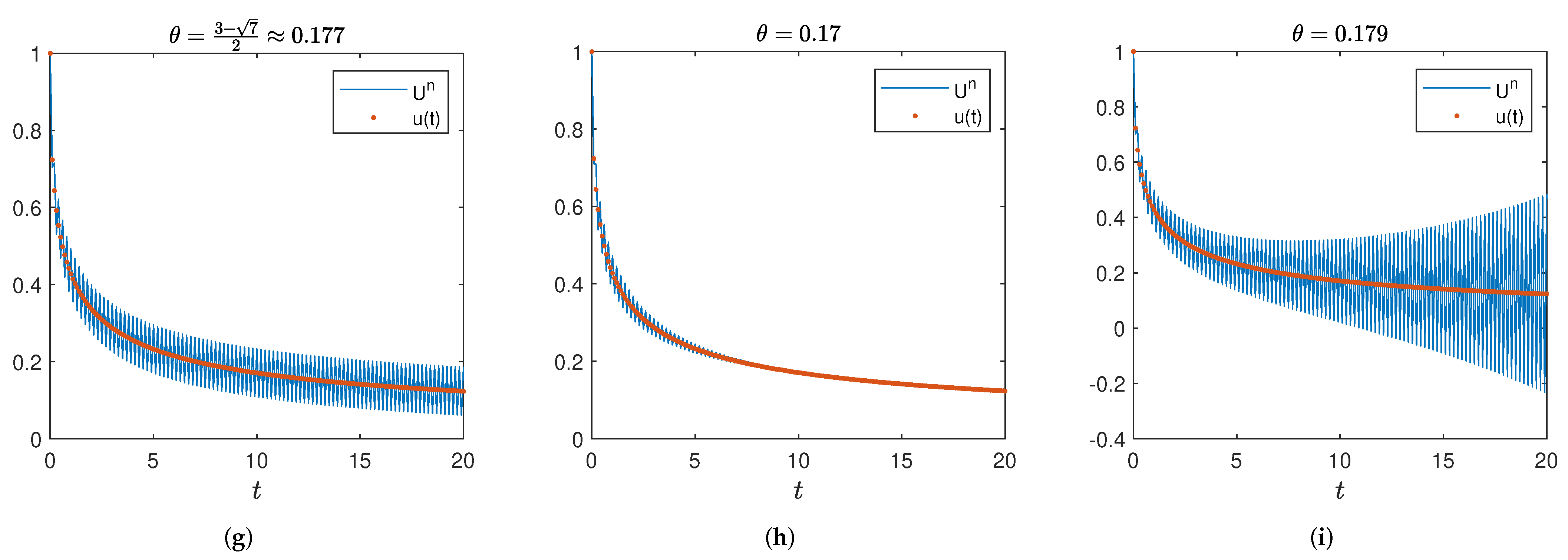
2.2. Stability Regions

Historically, Lubich [33] has proven that when using a convolution quadrature method (with a generating function $\tilde{\omega }\left(\zeta \right)={\sum }_{j=0}^{\infty }{\tilde{\omega }}_j{\zeta }^j$) to solve the linear Abel integral equation

$$u\left(t\right)=f\left(t\right)+\frac{\lambda }{\Gamma \left(\alpha \right)}{\int }_0^t{(t-s)}^{\alpha -1}u\left(s\right)\mathrm{d}s,$$

(8)

where $f\left(t\right)$ has finite limit as $t\to \infty$, the stability region S is precisely determined by

$$\mathbb{C}\setminus \{1/\tilde{\omega }\left(\zeta \right):|\zeta |\le 1\},$$

(9)

if the weights ${\tilde{\omega }}_n$ fulfill the following condition.

$${\tilde{\omega }}_n=\frac{n^{\alpha -1}}{\Gamma \left(\alpha \right)}+{\pi }_n,n\ge 1,\mathrm{with}\sum _{n=1}^{\infty }\left|{\pi }_n\right|<\infty .$$

(10)

Instead of (8), we concern ourselves in this work with the following fractional differential equation:

$${\partial }_t^{\alpha }u=\lambda u+g\left(t\right),\alpha \in (0,1)\mathrm{and}\Re \left(\lambda \right)<0,$$

(11)

where $g\left(t\right)$ decays exponentially and partially. Resorting to any ${\varpi }_p\left(\zeta \right)$ in CQ, the numerical scheme reads as follows:

$$\sum _{j=0}^n{\varpi }_{n-j}(U^j-U^0)=\overline{\tau }(U^n+\frac{1}{\lambda }{g}^n),n\ge n_0,$$

(12)

where $\overline{\tau }=\lambda {\tau }^{\alpha }$. We next identify conditions on ${\varpi }_j$ or its generating function ${\varpi }_p\left(\zeta \right)$ to determine the related stability region. It is worth noting that the first few steps ($n=1,2,\cdots ,n_0-1$) for (12) may need to be treated separately, e.g., by adding correction terms [9], to retain the high accuracy in cases where high-order methods are adopted.

Some assumptions on ${\varpi }_p\left(\zeta \right)$ are needed.

$$\begin{array}{cc}\hfill \left(\mathrm{A}1\right)& {\tau }^{-\alpha }{\varpi }_p\left(e^{-\tau }\right)-1=O\left({\tau }^p\right),\hfill \\ \hfill \left(\mathrm{A}2\right)& {\varpi }_p\left(\zeta \right)={(1-\zeta )}^{\alpha }\ell \left(\zeta \right),\ell \left(\zeta \right)\mathrm{is}\mathrm{nonzero}\mathrm{and}\mathrm{analytic}\mathrm{for}\zeta \in \{\zeta :|\zeta |\le 1\}.\hfill \end{array}$$

(13)

Note that the most well-known implicit CQ methods meet the assumptions (A1) and (A2), e.g., the fractional BDF-p and Newton–Gregory formula, among others. The assumption (A2) actually implies that ${\varpi }_n=O\left(n^{-\alpha -1}\right)$.

Given ${\varpi }_p\left(\zeta \right)$ that fulfills (A1) and (A2), introduce the sequence ${\left\{{\varpi }_j^{(-1)}\right\}}_{j=0}^{\infty }$ generated by $\frac{1}{{\varpi }_p\left(\zeta \right)}$. The next lemma shows that ${\tau }^{\alpha }{\sum }_{j=0}^n{\varpi }_j^{(-1)}{\varphi }^{n-j}$ is an approximation to $D_t^{-\alpha }\varphi$ at $t_n$. For a better presentation, the proof of the following lemmas in this section is left in Appendix A.

Lemma 2.

Let ${\varpi }_p\left(\zeta \right)$ satisfy the assumptions (A1) and (A2). Then, ${\tau }^{\alpha }{\sum }_{j=0}^n{\varpi }_j^{(-1)}{\varphi }^{n-j}$ approximates $\left(D_t^{-\alpha }\varphi \right)\left(t_n\right)$ with convergence order p, i.e., ${\varpi }_n^{(-1)}=O\left(n^{\alpha -1}\right)$ and ${\tau }^{\alpha }/{\varpi }_p\left(e^{-\tau }\right)-1=O\left({\tau }^p\right)$.

Lemma 3.

Let ${\varpi }_p\left(\zeta \right)$ satisfy the assumptions (A1) and (A2). The stability region S for (12) is determined by the following.

$$\mathbb{C} \backslash \{{\varpi }_p\left(\zeta \right):|\zeta |\le 1\}.$$

(14)

3. Novel Transformation Strategy

Instead of transformation (5) in which a polynomial-type function $\Theta (\zeta ;\theta )$ is involved, we shall, in this section, propose a different strategy by resorting to an exponential-type transform function and demonstrate that the new strategy is more robust by allowing a wider range of $\theta$ to guarantee the stability of schemes in solving fractional differential equations.

Let $\delta \left(\zeta \right)={\sum }_{j=1}^p\frac{1}{j}{(1-\zeta )}^j$ denote the generating function of backward difference formulas (BDF) of order $p\le 6$.

Theorem 1

(Exponential-type transformation). Let $\theta \in \mathbb{R}$ and assume ${\varpi }_p\left(\zeta \right)$ fulfills (A1) and (A2). Define the following:

$$\omega \left(\zeta \right)={\varpi }_p\left(\zeta \right)e^{\theta \delta \left(\zeta \right)},$$

(15)

then, the difference Formula (2) with weights generated by $\omega \left(\zeta \right)$ is convergent of order p.

Proof. 

Clearly, the function $e^{\theta \delta \left(\zeta \right)}$ (with respect to ζ) is analytic within the unit disc $\left|\zeta \right|<1$ and is k-times differentiable on the unit circle for any positive integer k; thus, its Fourier coefficients, i.e., the $e_n$ generated from $e^{\theta \delta \left(\zeta \right)}={\sum }_{n=0}^{\infty }{e}_n{\zeta }^n$, decay faster than, e.g., $O\left(n^{-k}\right)$. Then, the asymptotic property of ${\omega }_n$ is fully determined by ${\varpi }_n$, which, by assumption (A2), leads to the following.

$${\omega }_n=O\left(n^{-\alpha -1}\right).$$

(16)

Moreover, by the consistency condition of order p for ${\varpi }_p\left(\zeta \right)$ due to (A1) and that of $\delta \left(\zeta \right)$, the following holds.

$${\tau }^{-\alpha }{\varpi }_p\left(e^{-\tau }\right)=1+O\left({\tau }^p\right),{\tau }^{-1}\delta \left(e^{-\tau }\right)=1+O\left({\tau }^p\right).$$

Using the Taylor expansion, one immediately obtains the following:

$${\tau }^{-\alpha }{e}^{\theta \tau }\omega \left(e^{-\tau }\right)={\tau }^{-\alpha }{\varpi }_p\left(e^{-\tau }\right)e^{\theta \tau }{e}^{\theta \delta \left(e^{-\tau }\right)}=1+O\left({\tau }^p\right),$$

(17)

indicating that $\omega \left(\zeta \right)$, as a generating function in SCQ, is consistent of order p as well. Finally, by (16) and (17), we complete the proof of the theorem in accordance with Lemma 1. □

Remark 1.

In view of the fact that $\varphi \left(t_{n-\theta }\right)=\left(D_t^0\varphi \right)\left(t_{n-\theta }\right)$, Theorem 1 actually permits us to approximate $\varphi \left(t_{n-\theta }\right)$ by a discrete convolution.

$${\varphi }^{n-\theta }:=\sum _{j=0}^n{\theta }_j{\varphi }^{n-j},\mathit{where}{\theta }_j\mathit{is}\mathit{generated}\mathit{by}\sum _{j=0}^{\infty }{\theta }_j{\zeta }^j=e^{\theta \delta \left(\zeta \right)}.$$

(18)

As demonstrated in the arguments, ${\theta }_n$ decays faster than $O\left(n^{-k}\right)$ for any integer $k>0$. Indeed, since $e^{\theta \delta \left(\zeta \right)}$ is analytic for $\left|\zeta \right|<\rho$ for some $\rho >1$, ${\theta }_n$ decays exponentially.

For the purpose of application, it is of interest to present efficient algorithms to calculate the coefficients of $\omega \left(\zeta \right)$ in (15). The next lemma offers an algorithm by which ${\omega }_j$ can be obtained in a recursive manner.

Lemma 4.

Assume $\omega \left(\zeta \right)$ takes the form ${\left[P\left(\zeta \right)\right]}^{\alpha }{e}^{\theta Q\left(\zeta \right)}$ where $P\left(\zeta \right)$ and $Q\left(\zeta \right)$ are polynomials such that $\omega \left(\zeta \right)$ is analytic within the unit disc $\left|\zeta \right|<1$; then, we obtain the following:

$${\omega }_0={\left[P\left(0\right)\right]}^{\alpha }{e}^{\theta Q\left(0\right)},{\omega }_n=\frac{1}{nP\left(0\right)}\left[{\omega }_0{G}_{n-1}+\sum _{k=1}^{n-1}{\omega }_{n-k}\left(G_{k-1}-(n-k)P_k\right)\right],n\ge 1,$$

(19)

where $G_k$ includes the coefficients of $G\left(\zeta \right)$ defined by $G\left(\zeta \right)=\alpha P^{\prime }\left(\zeta \right)+\theta P\left(\zeta \right)Q^{\prime }\left(\zeta \right)$.

Proof. 

Take the derivative of $\omega \left(\zeta \right)={\left[P\left(\zeta \right)\right]}^{\alpha }{e}^{\theta Q\left(\zeta \right)}$ with respect to ζ and multiply both sides by $P\left(\zeta \right)$ to obtain the following.

$$P\left(\zeta \right){\omega }^{\prime }\left(\zeta \right)=\omega \left(\zeta \right)G\left(\zeta \right).$$

The Formula (19) then follows by taking the nth coefficient of both sides of the above equality. □

Remark 2.

It is notable that Algorithm (19) is efficient since $G\left(\zeta \right)$ and $P\left(\zeta \right)$ have finitely many nonzero coefficients; thus, the computing complexity to obtain ${\left\{{\omega }_j\right\}}_{j=0}^N$ is of $O\left(N\right)$.

In contrast to the polynomial-type transform function $\Theta (\zeta ;\theta )$ in (5), the exponential function $e^{\theta \delta \left(\zeta \right)}$ takes the advantage that it has no zero for any $\theta \in \mathbb{R}$, whence $e^{-\theta \delta \left(\zeta \right)}$ can always be expanded into a series without limiting the range of $\theta$. The immediate consequence is that in designing A($\vartheta$)-stable schemes, the exponential-type transform places no constraint on $\theta$ while the polynomial-type transform may limit the choice of $\theta$ severely, particularly for high-order methods.

To be more specific, consider the following simple trial equation:

$${\partial }_t^{\alpha }u=\lambda u,\alpha \in (0,1)\mathrm{and}\Re \left(\lambda \right)<0,$$

(20)

with initial condition $u\left(0\right)=u_0$. For a given generating function ${\varpi }_p\left(\zeta \right)$ that satisfies the Assumptions (A1) and (A2), by adopting the polynomial-type transform (5) or the exponential transform as in Theorem 1, one obtain the following discrete scheme:

$$\sum _{j=0}^n{\omega }_{n-j}(U^j-U^0)=\overline{\tau }{U}^{n-\theta },n\ge n_0,$$

(21)

where $\overline{\tau }=\lambda {\tau }^{\alpha }$ and $U^{n-\theta }={\sum }_{j=0}^n{\theta }_{n-j}{U}^j$. The weights ${\theta }_j$, depending on the choice of transform strategies, are coefficients of $\Theta (\zeta ;\theta )$ or $e^{\theta \delta \left(\zeta \right)}$, respectively.

Theorem 2.

Assume that ${\varpi }_p\left(\zeta \right)$ satisfies (A1) and (A2). For $\omega \left(\zeta \right)={\varpi }_p\left(\zeta \right)\Theta (\zeta ;\theta )$, the stability region S for (21) is determined by the following:

$$\mathbb{C} \backslash \{{\varpi }_p\left(\zeta \right):|\zeta |\le 1\},$$

(22)

provided that $\theta \in {\Lambda }_{\theta }:=\{\theta :\Theta (\zeta ;\theta )\ne 0\mathrm{for}\mathrm{all}|\zeta |\le 1\}$. In contrast, for $\omega \left(\zeta \right)={\varpi }_p\left(\zeta \right)e^{\theta \delta \left(\zeta \right)}$, stability region S is determined by (22) for any $\theta \in \mathbb{R}$.

Proof. 

Since $\Theta \left(\zeta \right)$ or $e^{\theta \delta \left(\zeta \right)}$ is analytic and nonzero for $\left|\zeta \right|\le 1$, $1/\Theta \left(\zeta \right)$ or $e^{-\theta \delta \left(\zeta \right)}$ can be expanded at $\zeta =0$ with coefficients ${\theta }_n^{(-1)}$ decay exponentially. By replacing n with k in the Equation (21) and multiplying both sides by ${\theta }_{n-k}^{(-1)}$ and summing k from $n_0$ to n, we obtain the following.

$$\sum _{k=n_0}^n{\theta }_{n-k}^{(-1)}\sum _{j=0}^k{\omega }_{k-j}(U^j-U^0)=\overline{\tau }\sum _{k=n_0}^n{\theta }_{n-k}^{(-1)}{U}^{k-\theta }.$$

(23)

By resorting to the fact that ${\varpi }_p\left(\zeta \right)=\omega \left(\zeta \right)\frac{1}{\Theta \left(\zeta \right)}$ or ${\varpi }_p\left(\zeta \right)=\omega \left(\zeta \right)e^{-\theta \delta \left(\zeta \right)}$ and Cauchy product of series, one can obtain the following:

$$\sum _{k=0}^n{\varpi }_{n-k}(U^k-U^0)=\overline{\tau }\left(U^n+\frac{1}{\lambda }{g}^n\right),$$

(24)

where $g^n$ takes the following form

$$g^n={\tau }^{-\alpha }\sum _{j=0}^{n_0-1}\left[\sum _{k=0}^{n_0-1-j}\left({\omega }_k-\lambda {\tau }^{\alpha }{\theta }_k\right){\theta }_{n-k-j}^{(-1)}\right]U^j-{\tau }^{-\alpha }{U}^0\sum _{j=0}^{n_0-1}\sum _{k=0}^{n_0-1-j}{\theta }_{n-k-j}^{(-1)}{\omega }_k,$$

indicating that $g^n$ decays exponentially. By comparing (24) with (12), one readily obtains result (22) from Lemma 3. □

Remark 3.

Several methods can be found in the literature [34] for determining ${\Lambda }_{\theta }$ explicitly. For example, resorting to the Schur criterion (see Schur polynomial in Appendix A, one can readily obtain the explicit form of ${\Lambda }_{\theta }$, as shown in

Table 1. Explicit form of ${\Lambda }_{\theta }$.

Order p	2	3	4
${\Lambda }_{\theta }$	$(-\infty ,\frac{1}{2})$	$(-\infty ,1-\frac{\sqrt{2}}{2})$	$(-\infty ,\frac{3}{2}-\frac{\sqrt{7}}{2})$

. The sharpness of the constraints on θ are verified in Example 1 of Section 5.

4. Applications

In this section, we apply the exponential-type transformation strategy to the following subdiffusion problem and demonstrate its advantages in developing robust numerical schemes:

$$\begin{array}{c}\hfill \left\{\begin{array}{cc}{\partial }_t^{\alpha }u(\mathbf{x},t)-\Delta u(\mathbf{x},t)=f(\mathbf{x},t),\hfill & (\mathbf{x},t)\in \mathrm{\Omega }\times (0,T],\hfill \\ u(\mathbf{x},t)=0,\hfill & \mathbf{x}\in \partial \mathrm{\Omega },t\in (0,T],\hfill \\ u(\mathbf{x},0)=v\left(\mathbf{x}\right),\hfill & \mathbf{x}\in \mathrm{\Omega },\hfill \end{array}\right.\end{array}$$

(25)

where the space $\mathrm{\Omega }\subset {\mathbb{R}}^d$$(d=1,2,3)$ is a bounded convex polygonal domain with the boundary denoted by $\partial \mathrm{\Omega }$. The operator $\Delta :D(\Delta )\to L^2\left(\mathrm{\Omega }\right)$ stands for the Laplacian with $D(\Delta )=H_0^1\left(\mathrm{\Omega }\right)\cap H^2\left(\mathrm{\Omega }\right)$ and $f:(0,T]\to L^2\left(\mathrm{\Omega }\right)$ is a given function. The initial function v, depending on its smoothness, belongs to $D(\Delta )$ or $L^2\left(\mathrm{\Omega }\right)$.

4.1. Formulation of Fully Discrete Scheme

In this section, we take $\delta \left(\zeta \right)=\frac{3}{2}-2\zeta +\frac{1}{2}{\zeta }^2$ and let ${\omega }_j$ be generated by $\omega \left(\zeta \right)={\left[\delta \left(\zeta \right)\right]}^{\alpha }{e}^{\theta \delta \left(\zeta \right)}$. In accordance with Theorem 1 (see also Remark 1), ${\varphi }^{n-\theta }$ and $D_{\tau ,\theta }^{\alpha ,n}\varphi$ both are of second-order accuracy relative to their continuous counterparts. To formulate the fully discrete scheme of the model, define the finite element space as follows:

$$V_h=\{{\chi }_h\in H_0^1\left(\Omega \right):{\chi }_h{|}_e\mathrm{is}\mathrm{a}\mathrm{linear}\mathrm{polynomial}\mathrm{function},e\in {\mathcal{T}}_h\}$$

where ${\mathcal{T}}_h$ is a shape regular and a quasi-uniform triangulation of $\mathrm{\Omega }$.

Let $P_h:L^2\left(\mathrm{\Omega }\right)\to V_h$ and $R_h:H_0^1\left(\mathrm{\Omega }\right)\to V_h$ stand for the $L^2\left(\mathrm{\Omega }\right)$ and Ritz projection, respectively, and define ${\Delta }_h:V_h\to V_h$ as the discrete Laplacian. By replacing $u\left(t\right)$ with $w\left(t\right)+v$ and $f\left(t\right)$ with $g\left(t\right)+f\left(0\right)$ in (25), the space semi-discrete scheme then reads as follows:

$$D_t^{\alpha }{w}_h\left(t\right)-{\Delta }_{h}w\left(t\right)=g_h\left(t\right)+f_h^0+{\Delta }_h{v}_h,$$

(26)

where $g_h:=P_{h}g$, $f_h^0=P_{h}f\left(0\right)$ and $v_h=R_{h}v$ if $v\in D(\Delta )$ or $v_h=P_{h}v$ if $v\in L^2\left(\mathrm{\Omega }\right)$. The fully discrete scheme can, thus, be stated as finding $W_h^n\in V_h$ such that the following is the case.

$$D_{\tau ,\theta }^{\alpha ,n}{W}_h-{\Delta }_h{W}_h^{n-\theta }=g_h^{n-\theta }+f_h^0+{\Delta }_h{v}_h,n\ge 1,\theta \in (-1,1).$$

(27)

In general cases, scheme (27) can only result in first-order convergence rates at positive times due to the initial singularity of the solution. We propose a modified scheme, with the motivation explained in the next section, by resorting to a single-step correction.

$$\begin{array}{c}\hfill D_{\tau ,\theta }^{\alpha ,1}{W}_h-{\Delta }_h{W}_h^{1-\theta }=(\theta +3/2)({\Delta }_h{v}_h+f_h^0)+g_h^{1-\theta },n=1,\\ \hfill D_{\tau ,\theta }^{\alpha ,n}{W}_h-{\Delta }_h{W}_h^{n-\theta }=g_h^{n-\theta }+f_h^0+{\Delta }_h{v}_h,n\ge 2.\end{array}$$

(28)

Note that for $\theta =-\frac{1}{2}$, the scheme (28) recovers exactly (27), indicating that (27) can resolve the initial singularity automatically if the problem is discretized at point $t_{n+\frac{1}{2}}$.

4.2. Optimal Error Estimates

The error estimate is based on solution representation and estimates of some kernels. Denote by $\widehat{\varphi }$ the Laplace transform of $\varphi$. Then, using the Laplace transform and its inverse transform, we obtain the following:

$$\begin{array}{cc}\hfill w_h\left(t\right)& =-\frac{1}{2\pi \mathrm{i}}{\int }_{{\Gamma }_{\sigma ,ϵ}}{e}^{zt}\left[K\left(z\right)({\Delta }_h{v}_h+f_h\left(0\right))+zK\left(z\right)\widehat{g_h}\left(z\right)\right]\mathrm{d}z,\hfill \end{array}$$

(29)

where $K\left(z\right)=-z^{-1}{(z^{\alpha }-{\Delta }_h)}^{-1}$ stands for the kernel function, and the contour (with the direction of an increasing imaginary part) ${\mathrm{\Gamma }}_{\sigma ,ϵ}$ is defined by the following.

$${\Gamma }_{\sigma ,ϵ}:=\{z\in \mathbb{C}:|z|=ϵ,|argz|\le \sigma \}\cup \{z\in \mathbb{C}:z=r{e}^{\pm \mathrm{i}\sigma },r\ge ϵ\}.$$

Theorem 3.

For $\alpha \in (0,1)$ and $\theta \in (-1,1)$, there exist ${\sigma }_0\in (\pi /2,\pi )$ and ${ϵ}_0>0$, both of which are free of α and τ such that for any $\sigma \in (\pi /2,{\sigma }_0)$ and any $ϵ<{ϵ}_0$, the solution of (28) takes the following form:

$$\begin{array}{c}\hfill W_h^n=-\frac{1}{2\pi \mathrm{i}}{\int }_{{\Gamma }_{\sigma ,ϵ}^{\tau }}{e}^{z{t}_n}\left[\ell \left(e^{-z\tau }\right)K\left({\delta }_{\tau }\left(e^{-z\tau }\right)\right)({\Delta }_h{v}_h+f_h^0)+\tau {\delta }_{\tau }\left(e^{-z\tau }\right)K\left({\delta }_{\tau }\left(e^{-z\tau }\right)\right)g_h\left(e^{-z\tau }\right)\right]\mathrm{d}z,\end{array}$$

(30)

where ${\mathrm{\Gamma }}_{\sigma ,ϵ}^{\tau }=\{z\in {\Gamma }_{\sigma ,ϵ}:|\Im \left(z\right)|\le \pi /\tau \}$, ${\delta }_{\tau }\left(\zeta \right)=\delta \left(\zeta \right)/\tau$ and $\ell \left(\zeta \right)=\delta \left(\zeta \right)\zeta \left(\frac{1}{1-\zeta }+\theta +\frac{1}{2}\right)e^{-\theta \delta \left(\zeta \right)}$.

Proof. 

Multiply both sides of (28) by ${\zeta }^n$ and sum the index n from 1 to ∞ to yield the following:

$$\sum _{n=1}^{\infty }{\zeta }^n{D}_{\tau ,\theta }^{\alpha ,n}{W}_h-\sum _{n=1}^{\infty }{\zeta }^n{\Delta }_h{W}_h^{n-\theta }=\sum _{n=1}^{\infty }{\zeta }^n{g}_h^{n-\theta }+(f_h^0+{\Delta }_h{v}_h)\left(\sum _{n=1}^{\infty }{\zeta }^n+(\theta +1/2)\zeta \right),$$

which leads to the following:

$$\left({\left[{\delta }_{\tau }\left(\zeta \right)\right]}^{\alpha }-{\Delta }_h\right)W_h\left(\zeta \right)=g_h\left(\zeta \right)+(f_h^0+{\Delta }_h{v}_h)\kappa \left(\zeta \right),$$

where $\kappa \left(\zeta \right)=\zeta \left(\frac{1}{1-\zeta }+\theta +\frac{1}{2}\right)e^{-\theta \delta \left(\zeta \right)}$. By Lemma B.1 in [22], for fixed constant ${\varphi }_0\in (\pi /2,\pi )$, there exists ${\sigma }_0\in (\pi /2,\pi )$, which depends only on ${\varphi }_0$ for any $\sigma \in (\pi /2,{\sigma }_0)$ and any $ϵ<{ϵ}_0$ where ${ϵ}_0$ is small enough, ${\delta }_{\tau }\left(e^{-z\tau }\right){|}_{z\in {\Gamma }_{\sigma ,ϵ}^{\tau }}\in {\Sigma }_{{\varphi }_0}:=\{z\in \mathbb{C}:|argz|<{\varphi }_0,z\ne 0\}$. By the Cauchy integral formula, we have the expression for $W_h^n$ by the following:

$$W_h^n=\frac{1}{2\pi \mathrm{i}}{\int }_{\left|\zeta \right|=\epsilon }\frac{W_h\left(\zeta \right)}{{\zeta }^{n+1}}\mathrm{d}\zeta \zeta =e^{-z\tau }\frac{\tau }{2\pi \mathrm{i}}{\int }_{{\Gamma }_{\epsilon }^{\tau }}{e}^{z{t}_n}{W}_h\left(e^{-z\tau }\right)\mathrm{d}z$$

where ${\mathrm{\Gamma }}_{\epsilon }^{\tau }:=\left\{z=-\frac{1}{\tau }ln\epsilon +\mathrm{i}y:y\in \mathbb{R},\left|y\right|\le \pi /\tau \right\}$. Let $\mathcal{L}$ be the region enclosed by contours ${\mathrm{\Gamma }}_{\sigma ,ϵ}^{\tau }$, ${\mathrm{\Gamma }}_{\epsilon }^{\tau }$, ${\mathrm{\Gamma }}_{\pm }^{\tau }:=\mathbb{R}\pm \mathrm{i}\pi /\tau$ (oriented from left to right); one can check whether $W_h\left(e^{-z\tau }\right)$ is analytic for $z\in \overline{\mathcal{L}}$. By using the Cauchy integral formula again and noting that the integral values along ${\mathrm{\Gamma }}_{-}^{\tau }$ and ${\mathrm{\Gamma }}_{+}^{\tau }$ are opposite, result (30) follows readily by taking $\ell \left(\zeta \right)=\tau {\delta }_{\tau }\left(\zeta \right)\kappa \left(\zeta \right)$. The proof is completed. □

Remark 4.

The arguments for Theorem 3 reveal the superiority of the exponential-type transformation strategy that, for any arbitrary θ, the transform function $e^{-\theta \delta \left(\zeta \right)}{|}_{\zeta =e^{-z\tau }}$ appearing in $\kappa \left(\zeta \right)$ is analytic for $z\in \overline{\mathcal{L}}$, in contrast to the polynomial-type transform function $\frac{1}{1-\theta +\theta \zeta }{|}_{\zeta =e^{-z\tau }}$ adopted in [25], which is singular at points $z=\pm \frac{\pi }{\tau }\in \overline{\mathcal{L}}$ when $\theta =\frac{1}{2}$ (in which case, the Crank–Nicolson scheme is excluded). See also [23,24] for similar situations. Therefore, the numerical scheme or numerical analysis is robust against shifted parameter θ when the exponential-type transformation strategy is considered. On the other hand, thanks to Theorem 1, function ${\delta }_{\tau }\left(\zeta \right)$ appearing in (30) is independent of α, allowing us to develop robust analyses even for small α. We argue that such types of robustness are not available for the schemes in [23,24,25] as ${\delta }_{\tau }\left(\zeta \right)$ in those schemes are singular at $\alpha =0$, leading to the blow-up of constants C in their estimates. See Example 3 in Section 5.

Lemma 5.

Let ${\Gamma }_{\sigma ,ϵ}^{\tau }$ be the contour defined in Theorem 3. For given $\theta \in (-1,1)$ and any $z\in {\mathrm{\Gamma }}_{\sigma ,ϵ}^{\tau }$, the following holds

$$|\ell \left(e^{-z\tau }\right)-1|\le C{\tau }^2{\left|z\right|}^2,$$

(31)

where C is independent of $\tau ,z$, but may be dependent on θ.

Proof. 

Since $\left|z\right|\tau \le \pi /sin\sigma <+\infty$, we only need to prove (31) for sufficiently small $\left|z\right|\tau$. By the expansion of $\ell \left(\zeta \right)$ at the point $\zeta =1$, we have the following: $\ell \left(\zeta \right)=1+c\left(\theta \right){(1-\zeta )}^2+{(1-\zeta )}^{3}r\left(\zeta \right),$ where $r\left(\zeta \right)$ is analytic at $\zeta =1$. One then immediately obtains the following: $\ell \left(e^{-z\tau }\right)=1+c\left(\theta \right){\tau }^2{\left|z\right|}^2+o({\tau }^2{\left|z\right|}^2)$, which completes the proof of the lemma. □

Theorem 4.

Suppose that $u_h\left(t\right):=w_h\left(t\right)+v_h$ is the solution of the space semi-discrete scheme of (25), and $U_h^n:=W_h^n+v_h$ is the solution of the fully discrete scheme of (25). If $f\in W^{1,\infty }(0,T;L^2\left(\mathrm{\Omega }\right))$ and ${\int }_0^t{(t-s)}^{\alpha -1}\parallel f^{\prime \prime }\left(x\right)\parallel \mathrm{d}s\in L^{\infty }(0,T)$ where $\parallel ·\parallel$ denotes the $L^2$ norm, then the following is the case:

$$\parallel U_h^n-u_h\left(t_n\right)\parallel \le C{\tau }^2\left(\mathcal{R}(t_n,v)+t_n^{\alpha -2}\parallel f\left(0\right)\parallel +t_n^{\alpha -1}\parallel f^{\prime }\left(0\right)\parallel +{\int }_0^{t_n}{(t_n-s)}^{\alpha -1}\parallel f^{″}\left(s\right)\parallel \mathrm{d}s\right),$$

(32)

where $\mathcal{R}(t_n,v)=t_n^{\alpha -2}\parallel \Delta v\parallel$ if $v\in D(\Delta )$ and $\mathcal{R}(t_n,v)=t_n^{-2}\parallel v\parallel$ if $v\in L^2\left(\mathrm{\Omega }\right)$. The constant C is independent of $\tau ,\alpha ,n,N$ and f but may depend on θ.

Proof. 

The technique for this theorem is quite standard and is essentially and partially based on Lemma 5 and the following estimates on ${\delta }_{\tau }\left(\zeta \right)$, which can be found in [22].

$$|{\delta }_{\tau }\left(e^{-z\tau }\right)-z|\le C{\tau }^2{\left|z\right|}^3,|{\delta }_{\tau }^{\alpha }\left(e^{-z\tau }\right)-z^{\alpha }|\le C{\tau }^2{\left|z\right|}^{2+\alpha },C_1\left|z\right|\le |{\delta }_{\tau }\left(e^{-z\tau }\right)|\le C_2\left|z\right|.$$

We omitted the details here for reasons of space. □

Remark 5.

The error $u-u_h$ of the space semi-discrete scheme (26) has been well studied by researchers and is not our main concern in this article. Interested readers can refer to [35] for more information.

5. Numerical Tests

Example 1.

In this example, we explore the stability of the numerical scheme (21):

$$\sum _{j=0}^n{\omega }_{n-j}(U^j-U^0)=\overline{\tau }{U}^{n-\theta },n\ge n_0,$$

for trial Equation (20) in which $n_0=1$ and the polynomial-type transformation is adopted and verify the sharpness of ${\Lambda }_{\theta }$ in Theorem 2. Let $\lambda =-1$, $\alpha =0.5$ and fix $\tau =0.1$. The exact solution of (20) can be expressed by the Mittag–Leffler function [6] $E_{\alpha }\left(x\right):={\sum }_{j=0}^{\infty }\frac{x^j}{\Gamma (j\alpha +1)}$, as $u\left(t\right)=u_0{E}_{\alpha }\left(\lambda t^{\alpha }\right)$.

In Figure 1, we illustrate the asymptotic properties of numerical solutions obtained under different θ for different numerical methods. The solutions in the first column are obtained under the threshold values $\theta =\frac{1}{2},\frac{2-\sqrt{2}}{2},\frac{3-\sqrt{7}}{2}$ (see Table 1) where one can observe, for each case, that the amplitude is invariant as time passes. By taking a smaller value of θ than its threshold, as shown in the middle column of Figure, we obtain numerical solutions that are asymptotically stable in contrast to the unbounded ones demonstrated in the last column in which θ exceeds the threshold a bit.

Example 2.

For the subdiffusion Problem (25), let $T=1$. Depending on the smoothness of v, we consider two cases:

(i) $f=0$, $v=sinx\in D(\Delta )$, $\mathrm{\Omega }=(0,\pi )$, with the exact solution $u(x,t)=E_{\alpha }(-t^{\alpha })sinx$;

(ii) $f=0$, $v={\chi }_{(0,1/2)}$, $\mathrm{\Omega }=(0,1).$

In

Table 2. $L^2$ error and convergence rates at time $t=0.5$ of Example 2 (i).

$\mathit{\alpha }$	$\mathit{\theta }$	Corrected Scheme (28)					Standard Scheme (27)
		$\mathit{\tau }=2^{-5}$	$\mathit{\tau }=2^{-6}$	$\mathit{\tau }=2^{-7}$	$\mathit{\tau }=2^{-8}$	Rates	$\mathit{\tau }=2^{-5}$	$\mathit{\tau }=2^{-6}$	$\mathit{\tau }=2^{-7}$	$\mathit{\tau }=2^{-8}$	Rates
	−0.9	4.33 × ${10}^{-6}$	3.10 × ${10}^{-6}$	6.92 × ${10}^{-7}$	1.62 × ${10}^{-7}$	2.09	7.50 × ${10}^{-4}$	3.91 × ${10}^{-4}$	1.96 × ${10}^{-4}$	9.82 × ${10}^{-5}$	1.00
0.1	−0.5	1.86 × ${10}^{-6}$	8.76 × ${10}^{-7}$	2.65 × ${10}^{-7}$	7.13 × ${10}^{-8}$	1.89	1.86 × ${10}^{-6}$	8.76 × ${10}^{-7}$	2.65 × ${10}^{-7}$	7.13 × ${10}^{-8}$	1.89
	0.5	1.47 × ${10}^{-4}$	3.43 × ${10}^{-5}$	8.27 × ${10}^{-6}$	2.02 × ${10}^{-6}$	2.03	2.02 × ${10}^{-3}$	9.97 × ${10}^{-4}$	4.95 × ${10}^{-4}$	2.47 × ${10}^{-4}$	1.01
	0.9	2.53 × ${10}^{-4}$	5.78 × ${10}^{-5}$	1.38 × ${10}^{-5}$	3.37 × ${10}^{-6}$	2.03	2.87 × ${10}^{-3}$	1.41 × ${10}^{-3}$	6.95 × ${10}^{-4}$	3.46 × ${10}^{-4}$	1.01
	−0.8	1.15 × ${10}^{-4}$	2.49 × ${10}^{-5}$	5.78 × ${10}^{-6}$	1.39 × ${10}^{-6}$	2.05	3.15 × ${10}^{-3}$	1.60 × ${10}^{-3}$	8.04 × ${10}^{-4}$	4.03 × ${10}^{-4}$	1.00
0.5	−0.5	3.86 × ${10}^{-5}$	6.97 × ${10}^{-6}$	1.44 × ${10}^{-6}$	3.24 × ${10}^{-7}$	2.15	3.86 × ${10}^{-5}$	6.97 × ${10}^{-6}$	1.44 × ${10}^{-6}$	3.24 × ${10}^{-7}$	2.15
	0	2.35 × ${10}^{-4}$	5.70 × ${10}^{-5}$	1.40 × ${10}^{-5}$	3.49 × ${10}^{-6}$	2.01	5.49 × ${10}^{-3}$	2.72 × ${10}^{-3}$	1.35 × ${10}^{-3}$	6.74 × ${10}^{-4}$	1.00
	0.6	2.35 × ${10}^{-4}$	5.70 × ${10}^{-5}$	1.40 × ${10}^{-5}$	3.49 × ${10}^{-6}$	2.01	1.23 × ${10}^{-2}$	6.02 × ${10}^{-3}$	2.98 × ${10}^{-3}$	1.49 × ${10}^{-3}$	1.01
	−0.5	2.35 × ${10}^{-4}$	5.70 × ${10}^{-5}$	1.40 × ${10}^{-5}$	3.49 × ${10}^{-6}$	2.01	3.05 × ${10}^{-4}$	7.23 × ${10}^{-5}$	1.76 × ${10}^{-5}$	4.35 × ${10}^{-6}$	2.02
0.9	−0.2	1.28 × ${10}^{-4}$	2.95 × ${10}^{-5}$	7.10 × ${10}^{-6}$	1.74 × ${10}^{-6}$	2.03	6.78 × ${10}^{-3}$	3.30 × ${10}^{-3}$	1.63 × ${10}^{-3}$	8.10 × ${10}^{-4}$	1.01
	0.3	3.56 × ${10}^{-4}$	8.65 × ${10}^{-5}$	2.14 × ${10}^{-5}$	5.31 × ${10}^{-6}$	2.01	1.78 × ${10}^{-2}$	8.72 × ${10}^{-3}$	4.33 × ${10}^{-3}$	2.15 × ${10}^{-3}$	1.01
	0.6	7.64 × ${10}^{-4}$	1.84 × ${10}^{-4}$	4.51 × ${10}^{-5}$	1.12 × ${10}^{-5}$	2.01	2.44 × ${10}^{-2}$	1.20 × ${10}^{-2}$	5.95 × ${10}^{-3}$	2.96 × ${10}^{-3}$	1.01

and

Table 3. $L^2$ error and convergence rates at time $t=0.5$ of Example 2 (ii).

$\mathit{\alpha }$	$\mathit{\theta }$	Corrected Scheme					Standard Scheme
		$\mathit{\tau }=2^{-5}$	$\mathit{\tau }=2^{-6}$	$\mathit{\tau }=2^{-7}$	$\mathit{\tau }=2^{-8}$	Rates	$\mathit{\tau }=2^{-5}$	$\mathit{\tau }=2^{-6}$	$\mathit{\tau }=2^{-7}$	$\mathit{\tau }=2^{-8}$	Rates
0.2	−0.5	2.68 × ${10}^{-6}$	7.74 × ${10}^{-7}$	2.03 × ${10}^{-7}$	5.14 × ${10}^{-8}$	1.98	2.68 × ${10}^{-6}$	7.74 × ${10}^{-7}$	2.03 × ${10}^{-7}$	5.14 × ${10}^{-8}$	1.98
	−0.3	7.66 × ${10}^{-6}$	1.92 × ${10}^{-6}$	4.80 × ${10}^{-7}$	1.18 × ${10}^{-7}$	2.02	9.41 × ${10}^{-5}$	4.69 × ${10}^{-5}$	2.28 × ${10}^{-5}$	1.07 × ${10}^{-5}$	1.09
	0	1.83 × ${10}^{-5}$	4.39 × ${10}^{-6}$	1.07 × ${10}^{-6}$	2.62 × ${10}^{-7}$	2.03	2.42 × ${10}^{-4}$	1.19 × ${10}^{-4}$	5.75 × ${10}^{-5}$	2.68 × ${10}^{-5}$	1.10
	0.9	7.69 × ${10}^{-5}$	1.75 × ${10}^{-5}$	4.14 × ${10}^{-6}$	9.97 × ${10}^{-7}$	2.06	7.07 × ${10}^{-4}$	3.40 × ${10}^{-4}$	1.63 × ${10}^{-4}$	7.56 × ${10}^{-5}$	1.11
0.8	−0.5	8.79 × ${10}^{-5}$	2.12 × ${10}^{-5}$	5.20 × ${10}^{-6}$	1.28 × ${10}^{-6}$	2.03	8.79 × ${10}^{-5}$	2.12 × ${10}^{-5}$	5.20 × ${10}^{-6}$	1.28 × ${10}^{-6}$	2.03
	0.1	1.99 × ${10}^{-4}$	4.64 × ${10}^{-5}$	1.12 × ${10}^{-5}$	2.71 × ${10}^{-6}$	2.04	7.59 × ${10}^{-4}$	3.95 × ${10}^{-4}$	1.95 × ${10}^{-4}$	9.18 × ${10}^{-5}$	1.09
	0.5	3.28 × ${10}^{-4}$	7.47 × ${10}^{-5}$	1.77 × ${10}^{-5}$	4.27 × ${10}^{-6}$	2.05	1.36 × ${10}^{-3}$	6.82 × ${10}^{-4}$	3.31 × ${10}^{-4}$	1.54 × ${10}^{-4}$	1.10
	0.7	4.11 × ${10}^{-4}$	9.26 × ${10}^{-5}$	2.18 × ${10}^{-5}$	5.25 × ${10}^{-6}$	2.06	1.68 × ${10}^{-3}$	8.29 × ${10}^{-4}$	3.99 × ${10}^{-4}$	1.86 × ${10}^{-4}$	1.10

, we present the$L^2$error and convergence rates for different α and θ for schemes (27) and (28), respectively. One observes that scheme (28) with correction terms results in optimal convergence rates while scheme (27) is of first-order accuracy except for$\theta =-0.5$, both of which are in line with our theoretical results.

Example 3.

We illustrate the robustness of (28) when $\alpha \to 0$ for subdiffusion Problem (25). Let $\mathrm{\Omega }=(0,\pi ),T=1$ and $u(x,t)=(E_{\alpha }(-t^{\alpha })+t^3)sinx$ such that $v=sinx\in D(\Delta )$. The source term is $f(x,t)=\left(6t^{3-\alpha }/\Gamma (4-\alpha )+t^3\right)sinx$. In Figure 2a, we illustrate the $L^2$ error of scheme (28) for varying α under different $\theta =-0.5,0.1,0.4,0.8$. In particular, the cases $\theta =0.1$ and $0.4$ of the scheme in [25] are also presented. Obviously, the scheme (28) is much more robust when $\alpha \to 0$ than the scheme in [25].

It may seem weird that, in (18), the term $\varphi \left(t_{n-\theta }\right)$ is approximated by a nonlocal formula with coefficients ${\theta }_j$ with $j=0,1,\cdots ,n$. We note that ${\theta }_j$ decays exponentially as plotted in Figure 2b, and in application, one can adopt only the first few values; e.g., the first 50 values will be sufficient to guarantee the accuracy.

6. Conclusions

A novel exponential-type transformation strategy is proposed to develop robust and accurate difference formulas for fractional derivatives by involving shifted parameter $\theta$. The advantages of this novel strategy over the polynomial type transform methods are explored in detail. As an application, the well-known fractional BDF-2 is transformed under the novel strategy and is adopted in the subdiffusion problem. Rigorous arguments are carried out, showing that the resultant scheme can resolve the solution initial singularity quite naturally at the special point $t_{n+\frac{1}{2}}$. The robustness for small $\alpha$ is also verified both theoretically and numerically.

References

1. Jin, B.; Lazarov, R.; Zhou, Z. Numerical methods for time-fractional evolution equations with nonsmooth data: A concise overview. Comput. Methods Appl. Mech. Eng. 2019, 346, 332–358. [Google Scholar] [CrossRef]
2. Metzler, R.; Klafter, J. The random walk’s guide to anomalous diffusion: A fractional dynamics approach. Phys. Rep. 2000, 339, 1–77. [Google Scholar] [CrossRef]
3. Feng, L.; Turner, I.; Perré, P.; Burrage, K. An investigation of nonlinear time-fractional anomalous diffusion models for simulating transport processes in heterogeneous binary media. Commun. Nonlinear Sci. Numer. Simul. 2021, 92, 105454. [Google Scholar] [CrossRef]
4. Povstenko, Y. Linear Fractional Diffusion-Wave Equation for Scientists and Engineers; Springer: Berlin/Heidelberg, Germany, 2015. [Google Scholar]
5. Wyss, W. The fractional diffusion equation. J. Math. Phys. 1986, 27, 2782–2785. [Google Scholar] [CrossRef]
6. Podlubny, I. Fractional Differential Equations: An Introduction to Fractional Derivatives, Fractional Differential Equations, to Methods of Their Solution and Some of Their Applications; Elsevier: Amsterdam, The Netherlands, 1998. [Google Scholar]
7. Lin, Y.; Xu, C. Finite difference/spectral approximations for the time-fractional diffusion equation. J. Comput. Phys. 2007, 225, 1533–1552. [Google Scholar] [CrossRef]
8. Sun, Z.Z.; Wu, X. A fully discrete difference scheme for a diffusion-wave system. Appl. Numer. Math. 2006, 56, 193–209. [Google Scholar] [CrossRef]
9. Lubich, C. Discretized fractional calculus. SIAM J. Math. Anal. 1986, 17, 704–719. [Google Scholar] [CrossRef]
10. Wang, Z.; Vong, S. Compact difference schemes for the modified anomalous fractional sub-diffusion equation and the fractional diffusion-wave equation. J. Comput. Phys. 2014, 277, 1–15. [Google Scholar] [CrossRef]
11. Zeng, F.; Zhang, Z.; Karniadakis, G.E. Second-order numerical methods for multi-term fractional differential equations: Smooth and non-smooth solutions. Comput. Methods Appl. Mech. Eng. 2017, 327, 478–502. [Google Scholar] [CrossRef]
12. Yin, B.; Liu, Y.; Li, H.; Zhang, Z. Two families of novel second-order fractional numerical formulas and their applications to fractional differential equations. arXiv 2019, arXiv:1906.01242. [Google Scholar]
13. Meerschaert, M.M.; Tadjeran, C. Finite difference approximations for fractional advection–dispersion flow equations. J. Comput. Appl. Math. 2004, 172, 65–77. [Google Scholar] [CrossRef]
14. Galeone, L.; Garrappa, R. Explicit methods for fractional differential equations and their stability properties. J. Comput. Appl. Math. 2009, 228, 548–560. [Google Scholar] [CrossRef]
15. Tian, W.; Zhou, H.; Deng, W. A class of second order difference approximations for solving space fractional diffusion equations. Math. Comput. 2015, 84, 1703–1727. [Google Scholar] [CrossRef]
16. Ding, H.; Li, C.; Yi, Q. A new second-order midpoint approximation formula for Riemann–Liouville derivative: Algorithm and its application. IMA J. Appl. Math. 2017, 82, 909–944. [Google Scholar] [CrossRef]
17. Yin, B.; Liu, Y.; Li, H. Necessity of introducing non-integer shifted parameters by constructing high accuracy finite difference algorithms for a two-sided space-fractional advection–diffusion model. Appl. Math. Lett. 2020, 105, 106347. [Google Scholar] [CrossRef]
18. Stynes, M. Too much regularity may force too much uniqueness. Fract. Calc. Appl. Anal. 2016, 19, 1554–1562. [Google Scholar] [CrossRef]
19. Sakamoto, K.; Yamamoto, M. Initial value/boundary value problems for fractional diffusion-wave equations and applications to some inverse problems. J. Math. Anal. Appl. 2011, 382, 426–447. [Google Scholar] [CrossRef]
20. Diethelm, K.; Garrappa, R.; Stynes, M. Good (and not so good) practices in computational methods for fractional calculus. Mathematics 2020, 8, 324. [Google Scholar] [CrossRef]
21. Yan, Y.; Khan, M.; Ford, N.J. An analysis of the modified L1 scheme for time-fractional partial differential equations with nonsmooth data. SIAM J. Numer. Anal. 2018, 56, 210–227. [Google Scholar] [CrossRef]
22. Jin, B.; Li, B.; Zhou, Z. Correction of high-order BDF convolution quadrature for fractional evolution equations. SIAM J. Sci. Comput. 2017, 39, A3129–A3152. [Google Scholar] [CrossRef]
23. Jin, B.; Li, B.; Zhou, Z. An analysis of the Crank–Nicolson method for subdiffusion. IMA J. Numer. Anal. 2018, 38, 518–541. [Google Scholar] [CrossRef]
24. Wang, J.; Wang, J.; Yin, L. A single-step correction scheme of Crank–Nicolson convolution quadrature for the subdiffusion equation. J. Sci. Comput. 2021, 87, 1–18. [Google Scholar] [CrossRef]
25. Yin, B.; Liu, Y.; Li, H.; Zhang, Z. Efficient shifted fractional trapezoidal rule for subdiffusion problems with nonsmooth solutions on uniform meshes. BIT Numer. Math. 2022, 62, 631–666. [Google Scholar] [CrossRef]
26. Liao, H.l.; McLean, W.; Zhang, J. A discrete gronwall inequality with applications to numerical schemes for subdiffusion problems. SIAM J. Numer. Anal. 2019, 57, 218–237. [Google Scholar] [CrossRef]
27. Liao, H.L.; Li, D.; Zhang, J. Sharp error estimate of the nonuniform L1 formula for linear reaction-subdiffusion equations. SIAM J. Numer. Anal. 2018, 56, 1112–1133. [Google Scholar] [CrossRef]
28. Liu, Y.; Yin, B.; Li, H.; Zhang, Z. The unified theory of shifted convolution quadrature for fractional calculus. J. Sci. Comput. 2021, 89, 1–24. [Google Scholar] [CrossRef]
29. Lubich, C. Convolution quadrature and discretized operational calculus. I. Numer. Math. 1988, 52, 129–145. [Google Scholar] [CrossRef]
30. Lubich, C. Convolution quadrature revisited. BIT Numer. Math. 2004, 44, 503–514. [Google Scholar] [CrossRef]
31. Yin, B.; Liu, Y.; Li, H. A class of shifted high-order numerical methods for the fractional mobile/immobile transport equations. Appl. Math. Comput. 2020, 368, 124799. [Google Scholar] [CrossRef]
32. Yin, B.; Liu, Y.; Li, H.; Zeng, F. A class of efficient time-stepping methods for multi-term time-fractional reaction-diffusion-wave equations. Appl. Numer. Math. 2021, 165, 56–82. [Google Scholar] [CrossRef]
33. Lubich, C. A stability analysis of convolution quadrature for Abel-Volterra integral equations. IMA J. Numer. Anal. 1986, 6, 87–101. [Google Scholar] [CrossRef]
34. Miller, J.J. On the location of zeros of certain classes of polynomials with applications to numerical analysis. IMA J. Appl. Math. 1971, 8, 397–406. [Google Scholar] [CrossRef]
35. Jin, B.; Lazarov, R.; Zhou, Z. Error estimates for a semidiscrete finite element method for fractional order parabolic equations. SIAM J. Numer. Anal. 2013, 51, 445–466. [Google Scholar] [CrossRef]
Figure 1. Justification of the sharpness of Theorem 2 when using the polynomial-type transform function Θ ( ζ ; θ ) for Example 1. (ac): exact solution u ( t ) vs. numerical solution U n obtained by the transformed 2nd-order Newton–Gregory formula. (df): exact solution u ( t ) vs. numerical solution U n obtained by the transformed 3rd-order Newton–Gregory formula. (gi): exact solution u ( t ) vs. numerical solution U n obtained by the transformed fractional BDF-4.
Fractalfract 06 00417 g001aFractalfract 06 00417 g001b
Figure 2. For Example 3. (a) Comparison of L 2 error between our scheme and that in [25] for different α . (b) Exponential decay of the weights | θ n | defined in (18).
Fractalfract 06 00417 g002