Dynamic Behavior Investigation of a Novel Epidemic Model Based on COVID-19 Risk Area Categorization

Abstract

This study establishes a compartment model for the categorized COVID-19 risk area. In this model, the compartments represent administrative regions at different transmission risk levels instead of individuals in traditional epidemic models. The county-level regions are partitioned into High-risk (H), Medium-risk (M), and Low-risk (L) areas dynamically according to the current number of confirmed cases. These risk areas are communicable by the movement of individuals. An LMH model is established with ordinary differential equations (ODEs). The basic reproduction number $R_0$ is derived for the transmission of risk areas to determine whether the pandemic is controlled. The stability of this LHM model is investigated by a Lyapunov function and Poincare–Bendixson theorem. We prove that the disease-free equilibrium ($R_0$ < 1) is globally asymptotically stable and the disease will die out. The endemic equilibrium ($R_0$ > 1) is locally and globally asymptotically stable, and the disease will become endemic. The numerical simulation and data analysis support the previous theoretical proofs. For the first time, the compartment model is applied to investigate the dynamics of the transmission of the COVID-19 risk area. This work should be of great value in the development of precision region-specific containment strategies.

1. Introduction

According to the viewpoints of some researchers, the COVID-19 pandemic seems to be approaching its end [1,2]. The COVID-19 pandemic is becoming endemic as the omicron variant can infect most populations rapidly. Hence, many governments have already lifted the stringent containment strategies such as mandatory isolation or quarantine. Public services have reopened, and travel restrictions have been relaxed. Compared to eliminating COVID-19 infections, some governments adopted mitigation strategies to minimize COVID-19 deaths by increasing vaccination rates and protecting the vulnerable [3].

In contrast, to prevent the spread of COVID-19 and minimize the related deaths, the Chinese government insists on very stringent containment policies [4]. Many accusations have been raised about the economic compromise and physical or mental sacrifices due to the intensive restrictions, in particular the “lockdown”. This study provides a new mathematical interpretation of a major Chinese containment strategy to avoid some misunderstandings. Based on the confirmed cases within the region, the county-level administrative divisions (counties or districts) are divided into three risk-related classifications (i.e., High-risk area, Medium-risk area, and Low-risk area). According to the document “Guidance on scientific prevention and precise control of the COVID-9 epidemic in a categorized manner” announced by the State Council of China [5], the districts with over 50 cumulative cases currently and a cluster of infected cases within 14 days are defined as High-risk areas. The districts with less than 50 cumulative cases or without a cluster of infected cases are defined as Medium-risk areas. The districts without confirmed cases are defined as Low-risk areas. Different containment policies are implemented in the three types of risk areas. In the High-risk areas, stringent strategies must be adopted to contain the spreading of COVID-19, and medical resources should be reinforced to save critically ill patients. However, in the Low-risk areas, social and economic activities are not affected. Only precautions such as face mask wearing are recommended to prevent potential COVID-19 transmissions.

Many studies have been carried out on the dynamics of COVID-19 transmission among populations [6,7]. However, few mathematical models focus on the effects of regional classification on the epidemic spreading. Often, compartment models established by ordinary differential equations (ODEs) or partial differential equations (PDEs) are employed to simulate the epidemic trends and analyze the effects of containment strategies indirectly [8,9,10]. In these models, individuals of the populations are divided into several compartments such as susceptible, infected, or more complex categories [11,12]. The effectiveness of non-pharmaceutical interventions is manifested by the variations of reproduction numbers, transmission parameters, and the number of infected cases.

Further, systems composed of SDEs or PDEs are established to achieve a better simulation for the realistic scenario, considering the spatial diffusion of the epidemic [13,14,15,16]. The parameters of the COVID-19 epidemic model vary with environmental fluctuations and stochasticity. It is reasonable to consider how environmental noise affects the transmission of COVID-19 epidemics. Thus, the SDE system adopts white noise to investigate the effect of stochastic environmental changes on the spreading of COVID-19 in the population. However, the basic ODE models must be investigated first since they are the framework and foundation of the SDE models. In the compartment models composed of PDE systems, the variation of individual compartments depends not only on time, but also on the different population densities. The effect of population density on the spread of COVID-19 has been analyzed. However, specific information related to both time and space is needed. The amount of data required is relatively large for the analysis, and the solutions are complicated. Thus, these studies based on PDE systems still remain at an early stage. Based on the established compartment models, the stability of these epidemic systems [17,18,19,20,21] is investigated to provide a theoretical foundation for the containment strategies.

In viewing the risk area classification and motivated by dividing individuals into different groups in a traditional compartment model, we establish an epidemic model to characterize the variation of COVID-19 risk areas. The regions of the same risk level are classified into a compartment instead of the individuals. The basic reproduction number $R_0$ is derived for the “transmission” among risk areas. To the best of our knowledge, no similar approaches have been established to study the implementation of containment strategies. Further, local and global stability analyses are carried out for this new system characterizing the transmission of regions.

The remaining part of this study is structured as follows: Section 2 introduces the LMH model and parameters. The stability of the disease-free and endemic equilibrium is investigated in Section 3. Data analysis is carried out in Section 4 to support the proof. We conclude this study in Section 5.

2. The LMH Model and Equilibrium

2.1. LMH Model Description

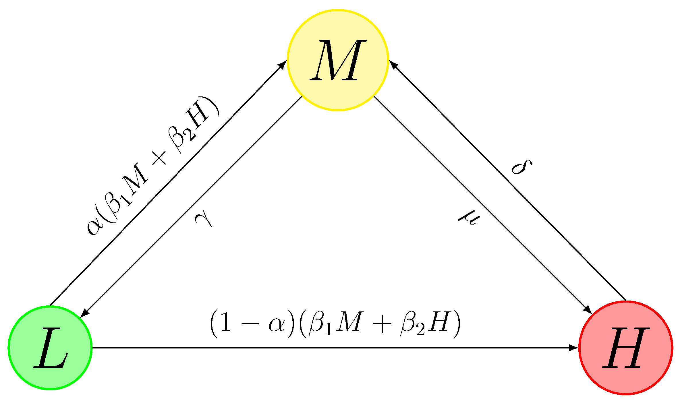
As described in the Introduction, three different levels of risk areas are divided based on the official standard from the disease control department (Figure 1). In this proof-of-concept model, a system established by ODEs is presented to characterize the dynamic behavior of the risk areas:

$$\left\{\begin{array}{ccc}\hfill \frac{\mathrm{d}L}{\mathrm{d}t}& =& -{\beta }_{1}ML-{\beta }_{2}HL+\gamma M\hfill \\ \hfill \frac{\mathrm{d}M}{\mathrm{d}t}& =& \alpha ({\beta }_{1}M+{\beta }_{2}H)L-\gamma M-\mu M+\delta H\hfill \\ \hfill \frac{\mathrm{d}H}{\mathrm{d}t}& =& (1-\alpha )({\beta }_{1}M+{\beta }_{2}H)L+\mu M-\delta H\hfill \end{array}\right.$$

(1)

where L, M, and H denote the number of Low-risk, Medium-risk, and High-risk areas at time t, respectively. ${\beta }_1$ represents the transition rate of Low-risk areas to Medium-risk areas by contacting the Medium-risk areas. The concept of “contact” is assumed to be the movement of unidentified individual cases between the areas in this model. ${\beta }_2$ represents the transition rate of Low-risk areas to Medium-risk areas by contacting the High-risk areas. $\alpha$ is the proportion of Low-risk areas transiting to Medium-risk areas, and $1-\alpha$ represents transiting to High-risk areas. $\mu$ and $\gamma$ are the transition rates from Medium-risk areas to High-risk and Low-risk areas. $\delta$ is the transition rate from High-risk areas to Medium-risk areas. In traditional epidemic models, the transition from one compartment to another is usually uni-directional. However, in this model, the interactions between compartments are reciprocal processes based on the containment policies, which brings more difficulties to investigating the stability of the system.

Since the number of the total county-level districts is a constant N, we set

$$x=\frac{L}{N},y=\frac{M}{N},z=\frac{H}{N}$$

(2)

$$\left\{\begin{array}{ccc}\hfill \frac{\mathrm{d}x}{\mathrm{d}t}& =& -{\beta }_{1}yx-{\beta }_{2}zx+\gamma y\hfill \\ \hfill \frac{\mathrm{d}y}{\mathrm{d}t}& =& \alpha ({\beta }_{1}y+{\beta }_{2}z)x-\gamma y-\mu y+\delta z\hfill \\ \hfill \frac{\mathrm{d}z}{\mathrm{d}t}& =& (1-\alpha )({\beta }_{1}y+{\beta }_{2}z)x+\mu y-\delta z\hfill \end{array}\right.$$

(3)

and

$$x+y+z=1.$$

(4)

2.2. Reproduction Number and Equilibrium of the Model

Disease-free equilibrium (DFE) is adopted from the traditional epidemic models. In this scenario dividing regions into different risk level areas, a DFE should illustrate that no Medium-risk or High-risk areas exist. By setting the derivatives of each compartment as zero, it can be derived:

$$\dot{x}=\dot{y}=\dot{z}=0.$$

(5)

A DFE of the system (3) always exists at

$${\mathrm{E}}_0=\left(1,0,0\right).$$

(6)

We also adopt the concept of the reproduction number (R) in this epidemic system. Here, the basic reproduction number ($R_0$) of System (1) is assumed to be the average number of uplifting risk areas by contact with a Medium- or High-risk area. $R_0$ is achieved as the spectral radius of $\mathcal{F}{\mathcal{V}}^{-1}$ ([22]):

$$F-V:F=\left[\begin{array}{cc}\alpha {\beta }_1& \alpha {\beta }_2\\ (1-\alpha ){\beta }_1& (1-\alpha ){\beta }_2\end{array}\right],V=\left[\begin{array}{cc}\gamma +\mu & -\delta \\ -\mu & \delta \end{array}\right]$$

(7)

$$R_0=\rho \left(F{V}^{-1}\right)=\frac{{\beta }_1}{\gamma }+\frac{{\beta }_2\mu }{\gamma \delta }+\frac{\eta {\beta }_2}{\delta }$$

(8)

where $\eta =1-\alpha$.

The system (1) has a unique DFE at ${\mathrm{E}}_0$ as $R_0⩽1$ and a unique endemic equilibrium (EE) at ${\mathrm{E}}^{*}$ as $R_0>1$. By solving (5), ${\mathrm{E}}^{*}$$(x^{*},y^{*},z^{*})$ can be derived when $R_0>1$:

$$x^{*}=\frac{1}{R_0},y^{*}=\frac{\delta }{\gamma \eta +\mu +\delta }\frac{R_0-1}{R_0},z^{*}=\frac{\gamma \eta +\mu }{\delta }{y}^{*}.$$

(9)

In the following section, the global stability of the DFE and EE is discussed. The biologically feasible domain for $(x,y,z)$ is

$$\Omega =\left\{(x,y,z)\in R_{+}^3:x+y+z=1\right\}$$

(10)

3. Global Stability of the DFE

Theorem 1.

The DFE ${\mathrm{E}}_0$ of System (3) is globally asymptotically stable if $R_0⩽1$.

Proof. 

A Lyapunov function is established by the following:

$${\mathcal{L}}_0=\frac{{\beta }_1}{\gamma }y+\frac{{\beta }_2\mu }{\delta \gamma }y+\frac{{\beta }_2}{\delta }z+\frac{{\beta }_1}{\gamma }z+\frac{{\beta }_2\mu }{\delta \gamma }z$$

(11)

The derivative of the Lyapunov function ${\mathcal{L}}_0$ can be derived

$$\begin{array}{cc}\hfill \frac{\mathrm{d}{\mathcal{L}}_0}{\mathrm{d}t}& ={\beta }_{1}y(\frac{{\beta }_1}{\gamma }x+\frac{{\beta }_2\alpha }{\delta }x+\frac{{\beta }_2\mu }{\delta \gamma }x-1)+{\beta }_{2}z(\frac{{\beta }_1}{\gamma }x+\frac{{\beta }_2\alpha }{\delta }x+\frac{{\beta }_2\mu }{\delta \gamma }x-1)\hfill \\ \hfill & =({\beta }_{1}y+{\beta }_{2}z)(x{R}_0-1)⩽0\hfill \end{array}$$

(12)

If $R_0<1$, the equality $\frac{\mathrm{d}{\mathcal{L}}_0}{\mathrm{d}t}=0$ implies that $y=z=0$ and yields $x=1$. Thus, the invariant set on which $\frac{\mathrm{d}{\mathcal{L}}_0}{\mathrm{d}t}$ only contains the point ${\mathrm{E}}_0$.

If $R_0=1$, the equality $\frac{\mathrm{d}{\mathcal{L}}_0}{\mathrm{d}t}=0$ implies that $x=1$. Thus, $y=0$ and $z=0$. As derived previously, each of the cases indicates that the DEF ${\mathrm{E}}_0$ is the only invariant set on $\{(x,y,z)\in \Omega :\frac{\mathrm{d}{\mathcal{L}}_0}{\mathrm{d}t}=0\}$.

Therefore, when $R_0<1$ or $R_0=1$, the largest invariant set on $\{(x,y,z)\in \Omega :\frac{\mathrm{d}{\mathcal{L}}_0}{\mathrm{d}t}=0\}$ always consists of the singleton ${\mathrm{E}}_0=(1,0,0)$. By LaSalle’s invariant principle, the DFE is globally asymptotically stable in $\Omega$ if $R_0⩽1$ □

4. Local and Global Stability of the EE

In this section, we applied Dulac’s criterion and the Poincare–Bendixson theorem to analyze the global stability of the EE of the system (3). At first, we set

$$x=1-y-z.$$

(13)

The system (3) can be converted to

$$\left\{\begin{array}{cc}\hfill \dot{y}& =-\alpha {\beta }_1{y}^2-(\alpha {\beta }_1+\alpha {\beta }_2)yz-\alpha {\beta }_2{z}^2+(\alpha {\beta }_1-\gamma -\mu )y+(\alpha {\beta }_2+\delta )z\hfill \\ \hfill \dot{z}& =-\eta {\beta }_1{y}^2-(\eta {\beta }_1+\alpha {\beta }_2)yz-\eta {\beta }_2{z}^2+(\eta {\beta }_1+\mu )y+(\eta {\beta }_2-\delta )z\hfill \end{array}\right.$$

(14)

Theorem 2.

The EE ${\mathrm{E}}^{*}$ of system (14) is locally asymptotically stable if $R_0>1$.

Proof. 

The Jacobian matrix for System (14) determined at ${\mathrm{E}}^{*}$ is

$$J\left(E^{*}\right)=\left[\begin{array}{cc}\alpha A-\gamma -\mu & \alpha B+\delta \\ \eta A+\mu & \eta B-\delta \end{array}\right]$$

(15)

where $\eta =1-\alpha$, $A={\beta }_1{x}^{*}-\gamma \frac{y^{*}}{x^{*}},B={\beta }_2{x}^{*}-\gamma \frac{y^{*}}{x^{*}}$. The characteristic equation of $J\left(E^{*}\right)$ is given by

$${\lambda }^2+(\delta -B+\gamma +\mu -A\alpha +B\alpha )\lambda -A\delta -B\gamma -B\mu +\delta \gamma +B\alpha \gamma =0$$

(16)

Due to

$$\delta +\gamma +\mu -A\alpha -\eta B=\frac{1}{{\beta }_1\delta +{\beta }_2\mu +\eta {\beta }_2\gamma }C+\frac{\gamma \delta }{\gamma \eta +\mu +\delta }(R_0-1)$$

(17)

and

$$-A\delta -B\gamma -B\mu +\delta \gamma +B\alpha \gamma =\delta \gamma (R_0-1),$$

(18)

where

$$C={\beta }_1{\delta }^2+{\beta }_1\delta \mu +\eta {\beta }_1\delta \gamma +{\beta }_2\mu \delta +{\beta }_2{\mu }^2+{\beta }_2\mu \gamma +\eta {\beta }_2\gamma \mu +\eta {\beta }_2{\gamma }^2.$$

(19)

Thus, the real part of the two roots of the above equation is negative if $R_0>1$. Hence, the EE ${\mathrm{E}}^{*}$ is locally asymptotically stable if $R_0>1$. □

Then, we shall prove the global stability of the EE $E^{*}$ whenever it exists, using the Dulac criterion and the Poincare–Bendixson theorem.

Theorem 3.

If $R_0>1$, the unique EE ${\mathrm{E}}^{*}$ of System (14) is globally asymptotically stable in the interior of Ω.

Proof. 

We first rule out periodic orbits in ${\Omega }^o$ using Dulac’s criterion [23,24]. We construct a Dulac function:

$$\Phi (y,z)=\frac{1}{yz},y>0,z>0.$$

(20)

The right-hand side of Equation (14) is represented by $P(y,z)$ and $Q(y,z)$. We have

$$\frac{\partial \Phi (y,z)P(y,z)}{\partial y}=-\alpha {\beta }_1\frac{1}{z}+\alpha {\beta }_2\frac{z}{y^2}-(\alpha {\beta }_2+\delta )\frac{1}{y^2}$$

(21)

$$\frac{\partial \Phi (y,z)Q(y,z)}{\partial z}=\eta {\beta }_1\frac{y}{z^2}-\eta {\beta }_2\frac{1}{y}-(\eta {\beta }_1+\mu )\frac{1}{z^2}$$

(22)

and

$$\begin{array}{cc}\hfill & \frac{\partial \Phi (y,z)P(y,z)}{\partial y}+\frac{\partial \Phi (y,z)Q(y,z)}{\partial z}\hfill \\ \hfill & =-\alpha {\beta }_1\frac{1}{z}+\alpha {\beta }_2\frac{z}{y^2}-(\alpha {\beta }_2+\delta )\frac{1}{y^2}+\eta {\beta }_1\frac{y}{z^2}-\eta {\beta }_2\frac{1}{y}-(\eta {\beta }_1+\mu )\frac{1}{z^2}\hfill \\ \hfill & =-\alpha {\beta }_1\frac{1}{z}+\alpha {\beta }_2\frac{z-1}{y^2}-\delta \frac{1}{y^2}+\eta {\beta }_1\frac{y-1}{z^2}-\eta {\beta }_2\frac{1}{y}-\mu \frac{1}{z^2}\hfill \\ \hfill & <0,\hfill \end{array}$$

(23)

for all $y>0$, $z>0$. Thus, System (14) does not have a limit cycle in ${\Omega }^o$. According to Theorem 2, if $R_0>1$ holds, then ${\mathrm{E}}^{*}$ is locally asymptotically stable. By applying the classical Poincare–Bendixson theorem [23], the unique EE ${\mathrm{E}}^{*}$ is globally asymptotically stable in $\Omega$. □

5. Data Analysis

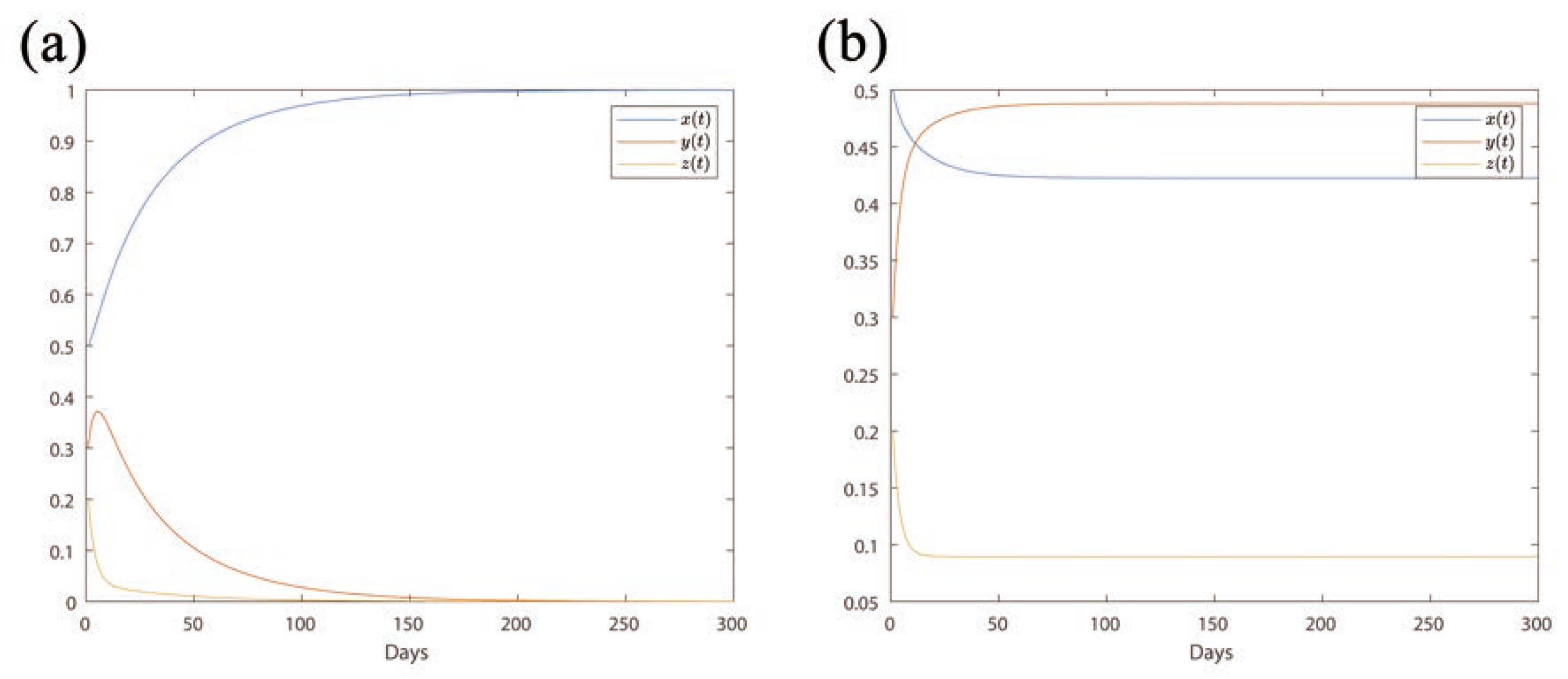
In this section, we conduct numerical simulations and real-world data application using this model. As demonstrated in Figure 2a, it can be noted that when $R_0<1$ ($R_0=0.47$), the proportions of Medium-risk (y) or High-risk (z) areas gradually approach 0 within half a year. The proportion of Low-risk areas (x) rises towards 1, indicating all areas will turn into Low-risk areas.

In the case $R_0>1$ ($R_0=2.37$; Figure 2b), the proportion of Low-risk areas x reaches 0.43 along with time (blue line); the proportion of Medium-risk areas y approaches 0.48 (orange line); the proportion of High-risk areas z reaches 0.09 (yellow line). The proportions of Medium- and High-risk areas approach stable non-zero values, illustrating that Medium- and High-risk areas will remain persistent.

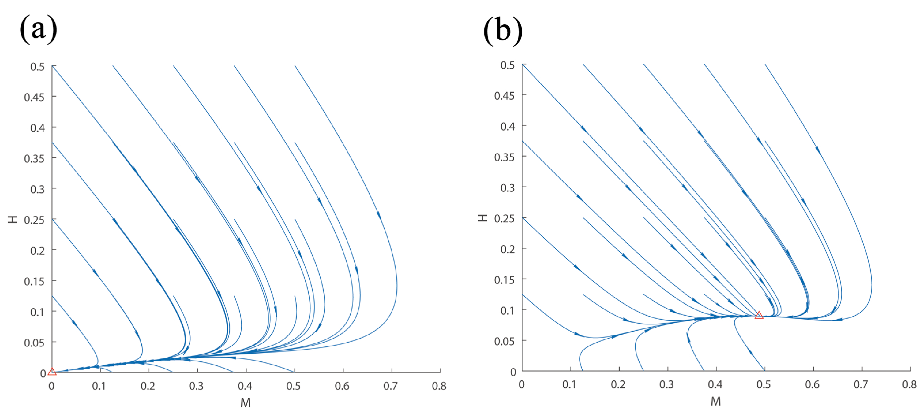
Further, the phase portraits of ($y,z$) lines are plotted in Figure 3 for $R_0<1(R_0=0.47)$ and $R_0>1(R_0=2.37)$. The horizontal axis denotes y, and the vertical axis denotes z. For any trajectories in Figure 3a, the ($y,z$) converges to ($0,0$). All the Medium- or High-risk areas will turn into Low-risk areas regardless of the initial conditions. The DFE point (1,0,0) is stable, as we proved in the previous section. On the other hand, at $R_0=2.37$, shown in Figure 3b, (y,z) trajectories approach the point (0.48,0.09). Hence, the High-risk and Medium-risk areas will persist and remain stable. As we proved, the solution of the system is an endemic equilibrium at $R_0$ > 1.

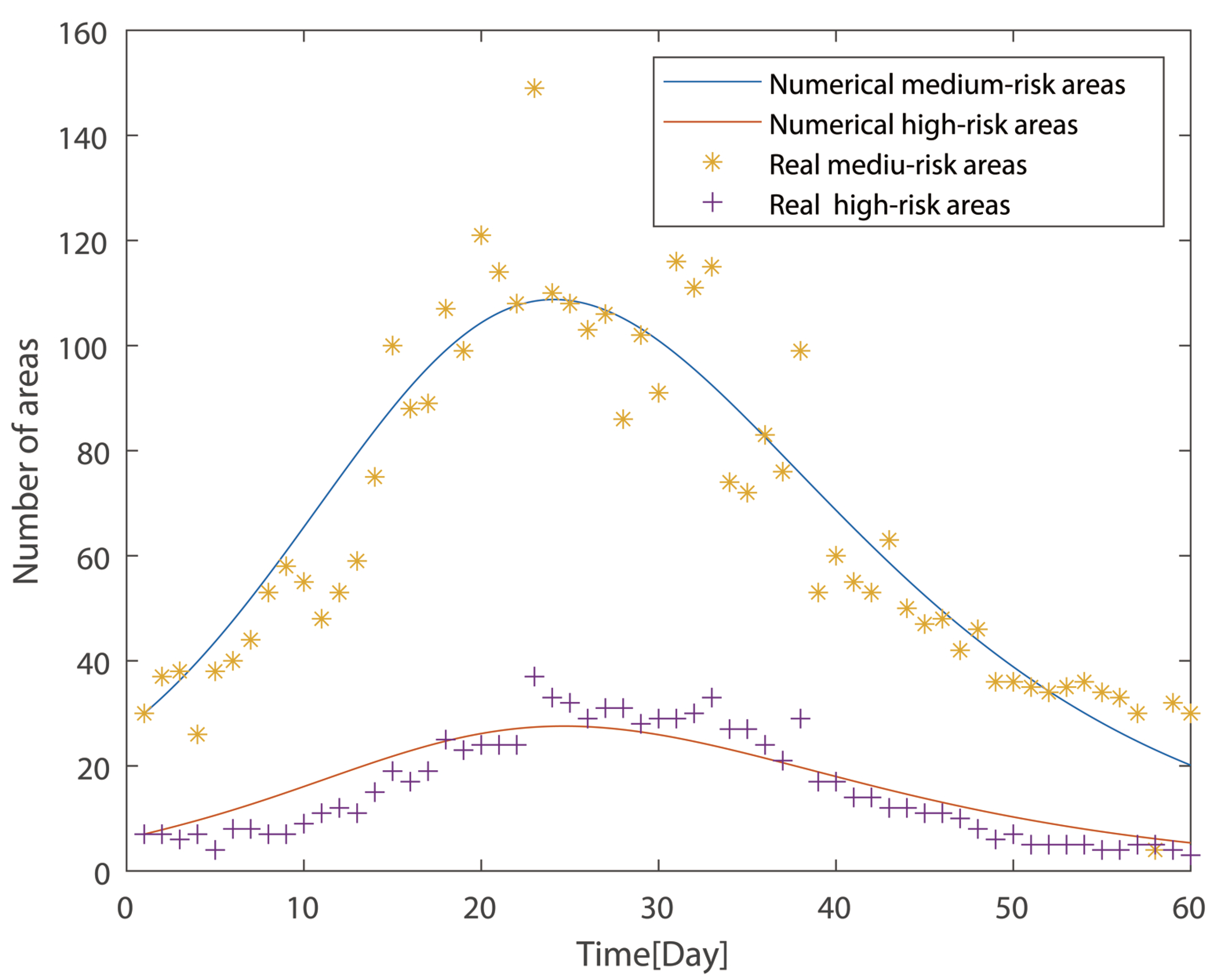
In addition, the real data in China were used to perform the simulation of the model (Figure 4). The High- and Medium-risk areas since 1 March 2022 for 60 days were collected from the Chinese National Council App [25]. The data were fit with the established LMH model using a nonlinear equation solver in MATLAB. The data are the variation of the proportion of Medium- and High-risk areas along with time. The yellow star dots represent the real proportion of Medium-risk areas, and the violet cross symbols represent the proportion of real High-risk areas. The lines are the data-fitting results of the LHM model. The blue line represents the numerical proportion of Medium-risk areas, and the red line is the proportion of High-risk areas. $R_0$ for the transmission of risk areas was determined to be 3.01 by the real data analysis. Since $R_0$ > 1, the High- or Medium-risk areas should persist, as proven in the previous section, which calls for a more effective containment policy if the goal is to achieve a disease-free equilibrium. Otherwise, if maintaining $R_0$ > 1, the containment strategies could be optimized to improve the efficiency of medical resources’ utilization at an endemic equilibrium and protect the vulnerable.

6. Discussion and Conclusions

In this work, we bring a novel approach to directly simulate the dynamics of risk area variation, as classified by the Chinese containment strategy. In this model, the same level of risk areas are denoted as one compartment, and the communication between the compartments is bi-directional. By using a similar idea as the epidemic compartment model, an LMH model was established to characterize the dynamic transition of areas with different levels of risk. The concept of the basic reproduction number was adopted for the transmission from Low-risk areas to Medium- or High-risk areas. We also determined two equilibria, DFE and EE. The stability analysis was carried out for the two equilibria. By constructing a Lyapunov function, the DFE was proven to be globally asymptotically stable for $R_0<1$. Using the Dulac criterion and the Poincare–Bendixson theorem, the global stability of the EE was obtained for $R_0>1$. After the proof, the Medium- or High-risk areas will decrease to 0 with $R_0<1$, but persist with $R_0>1$ in the numerical simulation. The stability of the two equilibria was also demonstrated by the convergence of trajectories in the phase portraits.

By this investigation, the application of the compartment model was extended for the epidemic transmission simulation for the first time to our knowledge. For healthcare policymakers, the division of risk areas with different control measures can facilitate the scheduling and optimization of medical resources under the assistance of this model. The data-driven model of risk regions should be used to adjust and predict the parameters related to epidemic containment. The containment strategy can be optimized for different levels of risk areas according to the spreading rate. Furthermore, the definition of High-, Medium-, and Low-risk regions can be adjusted according to the changes in risk regions with sufficient data and feedback from the calculated results. It is also possible to add more compartments to the model and change the parameters of the dynamical system for more precise control of High-risk areas spreading. Furthermore, the data and reference information obtained from the current epidemic modeling work should be informative for the next pandemic. Existing compartment models predict and control epidemic development among populations in an entire region. This current risk area transmission model is unique. It focuses on the development of the risk region, which can later be applied for adopting specific containment strategies according to the risk level. As for the case when this model should not be applied, first, local healthcare policymakers using the model should have the capacity to schedule and allocate medical resources (e.g., testing, vaccination, medical personnel, supplies, etc.). Furthermore, their willingness to deploy medical resources is essential. The authorities should not use the model without the capacity to allocate medical resources or insist on optimizing containment strategies.

As an initial investigation, this work suffers from some limitations. This ODE-based model can be used to analyze the dynamic change in the number of High-risk areas. In the following studies, PDEs can be applied to predict the spatial variation of High-risk areas. Furthermore, it should be noted that the risk area segregation becomes smaller and more precise. The current model is only for the initial validation and proof of concept. It can offer theoretical guidance for the analysis of a region-specific strategy in COVID-19 containment. This model is unique in analyzing the “transmission” of risk areas using a three-dimensional system. If the number of compartment groups is reduced, the model will become simpler, but the model’s accuracy may be sacrificed or it may not be able to provide guidance on specific containment strategies precisely for different areas. On the other hand, if adopting more risk region groupings, the model will become more complex, and the system’s dynamics will change accordingly. The theoretical proof and simulation driven by real-world data should be more challenging to investigate. Under a more effective and complex model, policymakers could optimize the containment strategies for different regions more precisely and allocate medical resources more efficiently under a more effective complex model. The risk areas should be smaller in an optimized model for precise control of a pandemic in future investigations.

References

- Murray, C.J. COVID-19 will continue but the end of the pandemic is near. Lancet 2022, 399, 417–419. [Google Scholar] [CrossRef]
- Katzourakis, A. COVID-19: Endemic doesn’t mean harmless. Nature 2022, 601, 485. [Google Scholar] [CrossRef] [PubMed]
- Mukaigawara, M.; Hassan, I.; Fernandes, G.; King, L.; Patel, J.; Sridhar, D. An equitable roadmap for ending the COVID-19 pandemic. Nat. Med. 2022, 28, 893–896. [Google Scholar] [CrossRef] [PubMed]
- National Health Commission and Others of the People. Protocol for prevention and control of COVID-19 (edition 6). China CDC Wkly. 2020, 2, 321. [Google Scholar] [CrossRef]
- The Joint Prevention and Control Mechanism of the State Council, State Council of China. Guidance on Scientific Prevention and Precise Control of the COVID-9 Epidemic in a Categorized Manner; Government Document; State Council of China: Beijing, China, 2020. (In Chinese) [Google Scholar]
- Grassly, N.C.; Pons-Salort, M.; Parker, E.P.; White, P.J.; Ferguson, N.M.; Ainslie, K.; Baguelin, M.; Bhatt, S.; Boonyasiri, A.; Brazeau, N.; et al. Comparison of molecular testing strategies for COVID-19 control: A mathematical modelling study. Lancet Infect. Dis. 2020, 20, 1381–1389. [Google Scholar] [CrossRef]
- He, Z.; Ren, L.; Yang, J.; Guo, L.; Feng, L.; Ma, C.; Wang, X.; Leng, Z.; Tong, X.; Zhou, W.; et al. Seroprevalence and humoral immune durability of anti-SARS-CoV-2 antibodies in Wuhan, China: A longitudinal, population-level, cross-sectional study. Lancet 2021, 397, 1075–1084. [Google Scholar] [CrossRef]
- Asamoah, J.K.K.; Jin, Z.; Sun, G.Q.; Seidu, B.; Yankson, E.; Abidemi, A.; Oduro, F.; Moore, S.E.; Okyere, E. Sensitivity assessment and optimal economic evaluation of a new COVID-19 compartmental epidemic model with control interventions. Chaos Solitons Fractals 2021, 146, 110885. [Google Scholar] [CrossRef]
- de León, U.A.P.; Pérez, Á.G.; Avila-Vales, E. An SEIARD epidemic model for COVID-19 in Mexico: Mathematical analysis and state-level forecast. Chaos Solitons Fractals 2020, 140, 110165. [Google Scholar] [CrossRef]
- Hussain, T.; Ozair, M.; Ali, F.; ur Rehman, S.; Assiri, T.A.; Mahmoud, E.E. Sensitivity analysis and optimal control of COVID-19 dynamics based on SEIQR model. Results Phys. 2021, 22, 103956. [Google Scholar] [CrossRef]
- Biala, T.A.; Khaliq, A. A fractional-order compartmental model for the spread of the COVID-19 pandemic. Commun. Nonlinear Sci. Numer. Simul. 2021, 98, 105764. [Google Scholar] [CrossRef]
- Bjørnstad, O.N.; Shea, K.; Krzywinski, M.; Altman, N. The SEIRS model for infectious disease dynamics. Nat. Methods 2020, 17, 557–559. [Google Scholar] [CrossRef] [PubMed]
- Grave, M.; Viguerie, A.; Barros, G.F.; Reali, A.; Coutinho, A.L. Assessing the spatio-temporal spread of COVID-19 via compartmental models with diffusion in Italy, USA, and Brazil. Arch. Comput. Methods Eng. 2021, 28, 4205–4223. [Google Scholar] [CrossRef] [PubMed]
- Niu, R.; Chan, Y.C.; Wong, E.W.; van Wyk, M.A.; Chen, G. A stochastic SEIHR model for COVID-19 data fluctuations. Nonlinear Dyn. 2021, 106, 1311–1323. [Google Scholar] [CrossRef] [PubMed]
- Viguerie, A.; Lorenzo, G.; Auricchio, F.; Baroli, D.; Hughes, T.J.; Patton, A.; Reali, A.; Yankeelov, T.E.; Veneziani, A. Simulating the spread of COVID-19 via a spatially-resolved susceptible–exposed–infected–recovered–deceased (SEIRD) model with heterogeneous diffusion. Appl. Math. Lett. 2021, 111, 106617. [Google Scholar] [CrossRef]
- Zhang, Z.; Zeb, A.; Hussain, S.; Alzahrani, E. Dynamics of COVID-19 mathematical model with stochastic perturbation. Adv. Differ. Equ. 2020, 2020, 451. [Google Scholar] [CrossRef]
- Annas, S.; Pratama, M.I.; Rifandi, M.; Sanusi, W.; Side, S. Stability analysis and numerical simulation of SEIR model for pandemic COVID-19 spread in Indonesia. Chaos Solitons Fractals 2020, 139, 110072. [Google Scholar] [CrossRef]
- Ansumali, S.; Kaushal, S.; Kumar, A.; Prakash, M.K.; Vidyasagar, M. Modelling a pandemic with asymptomatic patients, impact of lockdown and herd immunity, with applications to SARS-CoV-2. Annu. Rev. Control 2020, 50, 432–447. [Google Scholar] [CrossRef]
- Batabyal, S. COVID-19: Perturbation dynamics resulting chaos to stable with seasonality transmission. Chaos Solitons Fractals 2021, 145, 110772. [Google Scholar] [CrossRef]
- Jiao, J.; Liu, Z.; Cai, S. Dynamics of an SEIR model with infectivity in incubation period and homestead-isolation on the susceptible. Appl. Math. Lett. 2020, 107, 106442. [Google Scholar] [CrossRef]
- Pan, J.; Chen, Z.; He, Y.; Liu, T.; Cheng, X.; Xiao, J.; Feng, H. Why Controlling the Asymptomatic Infection Is Important: A Modelling Study with Stability and Sensitivity Analysis. Fractal Fract. 2022, 6, 197. [Google Scholar] [CrossRef]
- van den Driessche, P.; Watmough, J. Reproduction numbers and sub-threshold endemic equilibria for compartmental models of disease transmission. Math. Biosci. 2002, 180, 29–48. [Google Scholar] [CrossRef]
- Hale, J. Ordinary Differential Equations; John Wiley & Sons: Huntington, NY, USA, 1980. [Google Scholar]
- Hale, J.K.; Lunel, S.M.V. Introduction to Functional Differential Equations; Springer Science & Business Media: Berlin, Germany, 2013; Volume 99. [Google Scholar]
- State Council of China APP. Available online: https://app.www.gov.cn/download/English.html (accessed on 1 July 2022).