Article

Approximate Solution of Fractional Differential Equation by Quadratic Splines

1
School of Sciences, Shanghai Institute of Technology, Shanghai 201418, China
2
Ocean College, Zhejiang University, Hangzhou 310012, China
3
Village 1, East China Normal University, Shanghai 200062, China
4
School of Economics and Finance, Shanghai International Studies University, Shanghai 201620, China
*
Author to whom correspondence should be addressed.
Fractal Fract. 2022, 6(7), 369; https://doi.org/10.3390/fractalfract6070369
Submission received: 26 April 2022 / Revised: 18 June 2022 / Accepted: 20 June 2022 / Published: 30 June 2022

Abstract

:
In this article, we consider approximate solutions by quadratic splines for a fractional differential equation with two Caputo fractional derivatives, the orders of which satisfy 1 < α < 2 and 0 < β < 1 . Numerical computing schemes of the two fractional derivatives based on quadratic spline interpolation function are derived. Then, the recursion scheme for numerical solutions and the quadratic spline approximate solution are generated. Two numerical examples are used to check the proposed method. Additionally, comparisons with the L 1 L 2 numerical solutions are conducted. For the considered fractional differential equation with the leading order α , the involved undetermined parameters in the quadratic spline interpolation function can be exactly resolved.

1. Introduction

In recent decades, fractional calculus, due to its ability for modeling memory and hereditary properties of various materials and processes, has been applied to many fields of science and engineering, including relaxation and oscillation, viscoelasticity, anomalous diffusion, control problems, etc. [1,2,3,4,5,6,7,8]. At present, theories and applications of fractional calculus have attracted much interest and have become a vibrant research area. Fractional differential equations, including the existence, uniqueness and stability of solutions, were studied by some scholars [2,3,4,6,9,10]. In particular, new analytical and numerical methods were proposed [3,4,6,7,11,12,13]. Lie symmetry analysis and conservation laws were investigated for fractional evolution equations [14].
In [15], the difference method and its convergence for the space-time fractional advection–diffusion equation were investigated. In [16], a matrix representation of discrete analogues of fractional differentiation and integration was suggested and used to the numerical solution of fractional integral and differential equations. In [17], a local discontinuous Galerkin finite element method was suggested for Caputo-type fractional partial differential equations. In [18], a numerical Laplace transform technique was used to solve the irrational fractional-order systems. In [19,20,21], numerical methods based on spline functions were presented for the fractional differential equations. In [22], an Adams-type predictor–corrector method for the numerical solution of fractional differential equations was proposed. In [23], a numerical differentiation formula for the Caputo fractional derivative was developed by means of the quadratic interpolation approximation on three nodes. In [24], a survey and a MATLAB software tutorial for numerical methods were presented. In [25], Wang et al. proposed an asymptotic approximation method for a class of linear weakly singular Volterra integral equations based on the Laplace transform.
We recall the basic concepts in the fractional calculus. Let f ( t ) be piecewise continuous on ( 0 , + ) and integrable on any finite subinterval of ( 0 , + ) . The Riemann–Liouville fractional integral of f ( t ) has the definition
0 I t υ f ( t ) : = 0 t ( t τ ) υ 1 Γ ( υ ) f ( τ ) d τ , t > 0 ,
where υ is a positive real constant, and Γ ( · ) is Euler’s gamma function.
If f ( 0 + ) exists and f ( t ) is integrable on any finite subinterval of ( 0 , + ) , then applying the integration by parts in Equation (1), we have
0 I t υ f ( t ) = f ( 0 + ) t υ Γ ( υ + 1 ) + 0 t ( t τ ) υ Γ ( υ + 1 ) f ( τ ) d τ , t > 0 .
It follows that 0 I t υ f ( t ) f ( t ) as υ 0 + . So, we rationally define 0 I t 0 f ( t ) = f ( t ) for complementarity. The fractional integral satisfies the following equalities,
0 I t β 0 I t μ f ( t ) = 0 I t β + μ f ( t ) , β 0 , μ 0 , 0 I t ν t μ = Γ ( μ + 1 ) Γ ( μ + ν + 1 ) t μ + ν , ν 0 , μ > 1 .
The Riemann–Liouville fractional derivative of f ( t ) of order λ is defined, when it exists, as
0 D t λ f ( t ) : = d m d t m 0 I t m λ f ( t ) , t > 0 , m 1 < λ m , m N + ,
while the Caputo fractional derivative of f ( t ) of order λ is
0 D t λ f ( t ) : = 0 I t m λ f ( m ) ( t ) , t > 0 , m 1 < λ m , m N + .
From the definitions, for the Caputo fractional derivative of polynomial functions, the following equality holds
0 D t α ( a 0 t m 1 + a 1 t m 2 + + a m 1 ) = 0 , m 1 < α m ,
and for the power function t μ , μ > 0 , the Caputo fractional derivative is
0 D t α t μ = Γ ( μ + 1 ) Γ ( μ α + 1 ) t μ α , t > 0 , α > 0 and α < μ + 1 ,
where α denotes the least integer greater than or equal to α . We use the Caputo fractional derivative in this article in view of its convenience for formation of initial value condition. We denote the operators 0 I t λ as I t λ and 0 D t λ as D t λ for short.
In this article, we consider approximate solution by quadratic spline interpolation function for the initial value problem of the fractional differential equation with two Caputo fractional derivatives
D t α u ( t ) + c u ( t ) + b D t β u ( t ) + k u ( t ) = f ( t ) , 0 < t < T ,
u ( 0 ) = u 0 , u ( 0 ) = m 0 ,
where 1 < α < 2 , 0 < β < 1 , c , b , k , u 0 , m 0 are constants, and f ( t ) is a given continuous function on the interval [ 0 , T ] . In next section, we derive the quadratic spline interpolation function. In Section 3, the numerical schemes of the two fractional derivatives based on the quadratic spline interpolation are devised. In Section 4, the recursion scheme of numerical solutions for the fractional differential equation is generated. Two numerical examples are used to check the proposed method. Additionally, comparisons with the L 1 L 2 numerical solutions are conducted.

2. Quadratic Spline Interpolation Function

Suppose u ( t i ) , for i = 0 , 1 , , N , are known, where t i = i h and t N = T . Additionally, suppose m 0 = u ( 0 ) is known. Then, the quadratic spline interpolation function S ( t ) with the nodes t i , i = 0 , 1 , , N , satisfying S ( t i ) = u ( t i ) for i = 0 , 1 , , N and S ( 0 ) = u ( 0 ) , exists uniquely [26,27]. This means on each subinterval, [ t i , t i + 1 ] , S ( t ) is a quadratic polynomial,
S ( t ) = S i ( t ) , t [ t i , t i + 1 ] , i = 0 , 1 , , N 1 ,
and S ( t ) is continuous on the whole interval [ 0 , T ] .
First, we introduce the notations m i = S ( t i ) for i = 1 , 2 , , N , which serve as the interim parameters, to derive the quadratic spline interpolation function. Due to S ( t ) being a spline function of degree 1, interpolating the values ( t i , m i ) , i = 0 , 1 , , N , so S ( t ) has the form on the subinterval [ t i , t i + 1 ] ,
S ( t ) = S i ( t ) = t i + 1 t h m i + t t i h m i + 1 , t i t t i + 1 , i = 0 , 1 , , N 1 .
Operating indefinite integration leads to
S i ( t ) = ( t i + 1 t ) 2 2 h m i + ( t t i ) 2 2 h m i + 1 + C i , i = 0 , 1 , , N 1 ,
where C i are the integral constants. By setting
S i ( t i ) = u ( t i ) , i = 0 , 1 , , N 1 ,
we obtain C i = u ( t i ) + h 2 m i , i = 0 , 1 , , N 1 , and so Equation (5) becomes
S i ( t ) = u ( t i ) + h 2 m i ( t i + 1 t ) 2 2 h m i + ( t t i ) 2 2 h m i + 1 , i = 0 , 1 , , N 1 .
The parameters m i , i = 1 , 2 , , N , may be determined by the continuity of the function S ( t ) on the interval [ 0 , T ] as
S i ( t i + 1 ) = u ( t i + 1 ) , i = 0 , 1 , , N 1 .
Applying the condition to Equation (6), we have
m i + 1 + m i = 2 h ( u ( t i + 1 ) u ( t i ) ) , i = 0 , 1 , , N 1 .
By the iterations in Equation (7), we give expressions to each m i , i = 1 , 2 , , N , in terms of m 0 , u ( t 0 ) , u ( t 1 ) , , u ( t i ) as
m 1 = 2 h ( u ( t 0 ) + u ( t 1 ) ) m 0 , m 2 = 2 h ( u ( t 0 ) 2 u ( t 1 ) + u ( t 2 ) ) + m 0 , m 3 = 2 h ( u ( t 0 ) + 2 u ( t 1 ) 2 u ( t 2 ) + u ( t 3 ) ) m 0 , .
The general form is
m i = ( 1 ) i 2 u ( t 0 ) h + 4 h j = 1 i 1 ( 1 ) i j u ( t j ) + 2 h u ( t i ) + ( 1 ) i m 0 , i = 1 , 2 , , N ,
where the sum Σ vanishes if i = 1 .
Substituting Equation (8) into Equation (6), we obtain the quadratic spline interpolation function S ( t ) on the subinterval [ t i , t i + 1 ] expressed through m 0 , u ( t 0 ) , u ( t 1 ) , , u ( t i + 1 ) ,
S i ( t ) = u ( t i ) + h 2 ( t i + 1 t ) 2 2 h ( 1 ) i 2 u ( t 0 ) h + 4 h j = 1 i 1 ( 1 ) i j u ( t j ) + 2 h u ( t i ) + ( 1 ) i m 0 + ( t t i ) 2 2 h ( 1 ) i + 1 2 u ( t 0 ) h + 4 h j = 1 i ( 1 ) i + 1 j u ( t j ) + 2 h u ( t i + 1 ) + ( 1 ) i + 1 m 0 , i = 0 , 1 , , N 1 .
We indicate that due to m i , i = 0 , 1 , 2 , , N , are constants, Equations (4) and (6) will be used in the numerical computing process of fractional derivatives, and the expression of m i in Equation (8) will be substituted at the final procedure to avoid large expressions by using Equation (9).
For estimation of interpolation remainder R ( t ) = u ( t ) S ( t ) , it was proved that if u ( t ) C 3 [ 0 , T ] with u ( 3 ) ( t ) of bounded variation, then there exists M > 0 such that [26,27]
R ( j ) ( t ) = sup 0 t T R ( j ) ( t ) M h 3 j , j = 0 , 1 , 2 .
Li and Huang [28] proved the result under the assumption u ( t ) C 4 [ 0 , T ] .

3. Numerical Computation of Fractional Derivatives

We calculate numerically the fractional derivatives D t α u ( t ) ( 1 < α < 2 ) and D t β u ( t ) ( 0 < β < 1 ) at each nodes t = t i , i = 1 , 2 , , N , using the quadratic spline interpolation function S ( t ) . First, the α -th order derivative is approximated as
D t α u ( t ) t i D t α S ( t ) t i = I t 2 α S ( t ) t i = 0 t i ( t i z ) 1 α Γ ( 2 α ) S ( z ) d z .
Form Equation (4), S ( t ) is piecewise constants on the interval [ 0 , T ] , and has the form on the interval ( t i , t i + 1 ) as
S i ( t ) = m i + 1 m i h , t i < t < t i + 1 , i = 0 , 1 , , N 1 .
Integrating piecewise in Equation (11) and applying Equation (12) yield
D t α S ( t ) t i = j = 0 i 1 t j t j + 1 ( t i z ) 1 α Γ ( 2 α ) S j ( z ) d z = j = 0 i 1 ( t i t j + 1 ) 2 α ( t i t j ) 2 α h Γ ( 3 α ) ( m j m j + 1 ) .
Substituting t j = j h leads to
D t α S ( t ) t i = h 1 α Γ ( 3 α ) j = 0 i 1 ( ( i j 1 ) 2 α ( i j ) 2 α ) ( m j m j + 1 ) .
Regrouping the right hand side leads to the following equation
D t α S ( t ) t i = h 1 α Γ ( 3 α ) j = 0 i w i , j α m j ,
where
w i , 0 α = ( i 1 ) 2 α i 2 α , w i , j α = ( i j 1 ) 2 α 2 ( i j ) 2 α + ( i j + 1 ) 2 α , 1 j i 1 , w i , i α = 1 .
Substituting the derivatives m j , j = 1 , 2 , , i , in Equation (8) into Equation (14), we obtain the fractional derivative of order α at t = t i in terms of m 0 , u ( t 0 ) , u ( t 1 ) , , u ( t i ) as
D t α u ( t ) t i D t α S ( t ) t i = 2 h α Γ ( 3 α ) h 2 λ i α m 0 + u ( t i ) + j = 0 i 1 ρ i , j α u ( t j ) ,
where
ρ i , 0 α = j = 1 i ( 1 ) j w i , j α , λ i α = w i , 0 α + ρ i , 0 α , ρ i , j α = w i , j α + 2 l = j + 1 i ( 1 ) l j w i , l α , j = 1 , 2 , , i 1 .
For the β -th order fractional derivative D t β u ( t ) at t = t i , in a similar manner, we have
D t β u ( t ) t i D t β S ( t ) t i = 0 t i ( t i z ) β Γ ( 1 β ) S ( z ) d z = j = 0 i 1 t j t j + 1 ( t i z ) β Γ ( 1 β ) S j ( z ) d z .
Instead, here S j ( z ) is a linear function as in Equation (4). The sub-domain integration is calculated as
t j t j + 1 ( t i z ) β Γ ( 1 β ) S j ( z ) d z = t j t j + 1 ( t i z ) β Γ ( 1 β ) t j + 1 z h m j + z t j h m j + 1 d z = h 1 β Γ ( 3 β ) ( ( i j 1 ) 2 β ( i j 2 + β ) ( i j ) 1 β ) m j + ( ( i j ) 2 β ( i j + 1 β ) ( i j 1 ) 1 β ) m j + 1 .
Substituting it into Equation (18) and regrouping according to m j lead to
D t β S ( t ) t i = h 1 β Γ ( 3 β ) j = 0 i w i , j β m j ,
where
w i , 0 β = ( i 1 ) 2 β ( i 2 + β ) i 1 β , w i , j β = ( i j 1 ) 2 β 2 ( i j ) 2 β + ( i j + 1 ) 2 β , 1 j i 1 , w i , i β = 1 .
Substituting the derivatives m j , j = 1 , 2 , , i , in Equation (8) into Equation (19), we obtain the fractional derivative of order β at t = t i in terms of m 0 , u ( t 0 ) , u ( t 1 ) , , u ( t i ) as
D t β u ( t ) t i D t β S ( t ) t i = 2 h β Γ ( 3 β ) h 2 λ i β m 0 + u ( t i ) + j = 0 i 1 ρ i , j β u ( t j ) ,
where
ρ i , 0 β = j = 1 i ( 1 ) j w i , j β , λ i β = w i , 0 β + ρ i , 0 β , ρ i , j β = w i , j β + 2 l = j + 1 i ( 1 ) l j w i , l β , j = 1 , 2 , , i 1 .
We remark for the two fractional derivatives that the integral in Equation (18) is a little more tactical than that in Equation (13), and w i , 0 β in Equation (20) has a different form compared with w i , 0 α in Equation (15). Nevertheless, except the expressions of w i , 0 α and w i , 0 β , the expressions in Equations (19)–(22) present the same layouts as in Equations (14)–(17).
For the error estimation, from Equation (10) we have
D t α u ( t ) t i D t α S ( t ) t i I t 2 α u ( t ) S ( t ) t i M t i 2 α h Γ ( 3 α ) ,
and
D t β u ( t ) t i D t β S ( t ) t i I t 1 β u ( t ) S ( t ) t i M t i 1 β h 2 Γ ( 2 β ) ,
for i = 1 , 2 , , N .

4. Solution of Fractional Differential Equation

At t = t i , the fractional differential Equation (2) becomes
D t α u ( t ) t i + c u ( t i ) + b D t β u ( t ) t i + k u ( t i ) = f i , i = 1 , 2 , , N ,
where f i = f ( t i ) , i = 1 , 2 , , N , are known values. Approximating the two fractional derivatives and the first order derivative by the counterparts of the quadratic spline interpolation function S ( t ) yields
D t α S ( t ) t i + c S ( t i ) + b D t β S ( t ) t i + k u ( t i ) + E R ( u , t i ) = f i , i = 1 , 2 , , N ,
where the truncation error is estimated from Equations (10), (23) and (24) as
| E R ( u , t i ) | M t i 2 α h Γ ( 3 α ) + c M h 2 + b M t i 1 β h 2 Γ ( 2 β ) ,
where M is a constant related to u ( t ) .
Inserting the results about the derivative m i = S ( t i ) in Equation (8) and the fractional derivatives in Equations (16) and (21) into Equation (25), we have
2 h α Γ ( 3 α ) h 2 λ i α m 0 + u ( t i ) + j = 0 i 1 ρ i , j α u ( t j ) + 2 c h ( 1 ) i u ( t 0 ) + 2 j = 1 i 1 ( 1 ) i j u ( t j ) + u ( t i ) + ( 1 ) i c m 0 + 2 b h β Γ ( 3 β ) h 2 λ i β m 0 + u ( t i ) + j = 0 i 1 ρ i , j β u ( t j ) + k u ( t i ) + E R ( u , t i ) = f i .
Leaving out the error term E R ( u , t i ) and replacing u ( t i ) by their numerical approximations u i , we obtain the recursion scheme of the numerical approximations u i , i = 1 , 2 , , N , from m 0 , u 0 , u 1 , , u i 1 as
u i = 2 h α Γ ( 3 α ) + 2 c h + 2 b h β Γ ( 3 β ) + k 1 f i h 1 α Γ ( 3 α ) λ i α + ( 1 ) i c + b h 1 β Γ ( 3 β ) λ i β m 0 2 h α Γ ( 3 α ) ρ i , 0 α + ( 1 ) i 2 c h + 2 b h β Γ ( 3 β ) ρ i , 0 β u 0 j = 1 i 1 2 h α Γ ( 3 α ) ρ i , j α + ( 1 ) i j 4 c h + 2 b h β Γ ( 3 β ) ρ i , j β u j , i = 1 , 2 , , N .
Thus the recursion scheme (27) gives the numerical solutions u 0 , u 1 , , u N , derived from quadratic splines, and Equation (9) gives the quadratic spline approximate solution by replacing u ( t j ) by u j , j = 1 , 2 , , N .
We will compare the present algorithm with the usual L 1 L 2 algorithm to approximate the fractional derivatives D t α u ( t ) and D t β u ( t ) [1,23]. We note that the L 2 method utilizes the quadratic interpolation polynomials on three nodes to approximate the function u ( t ) , while the L 1 method approximate the function u ( t ) by using piecewise linear interpolation. So for the present problem, Equations (2) and (3), the first two node values need to be given as the iterative initial values in the L 1 L 2 numerical solutions.
On the interval [ t j , t j + 1 ] , j = 1 , 2 , , N 1 , approximate u ( t ) by the quadratic interpolation polynomials j ( t ) on the nodes t j 1 , t j , t j + 1 , while on the first interval [ t 0 , t 1 ] , u ( t ) is approximated by 1 ( t ) . Thus, the L 2 method derives the following approximation for the fractional derivative:
D t α u ( t ) t i u ( t 0 ) 2 u ( t 1 ) + u ( t 2 ) h α Γ ( 3 α ) i 2 α ( i 1 ) 2 α + j = 1 i 1 u ( t j 1 ) 2 u ( t j ) + u ( t j + 1 ) h α Γ ( 3 α ) ( i j ) 2 α ( i j 1 ) 2 α , i 2 .
The first-order derivative is also approximated by using the quadratic interpolation polynomials as u ( t i ) i 1 ( t ) for i 2 . For the fractional derivative of order β , using the L 1 method we have
D t β u ( t ) t i j = 0 i 1 u ( t j + 1 ) u ( t j ) ) h β Γ ( 2 β ) ( i j ) 1 β ( i j 1 ) 1 β , i 1 .
Thus, by discretizing Equation (2) at t i , i 2 , and using Equations (28) and (29), the L 1 L 2 numerical solutions are obtained as
u ^ 0 = u ( 0 ) , u ^ 1 = u ( 0 ) + h u ( 0 ) ,
u ^ 2 = 2 2 α h α Γ ( 3 α ) + 3 c 2 h + k + b h β Γ ( 2 β ) 1 f 2 ( u ^ 0 2 u ^ 1 ) 2 2 α h α Γ ( 3 α ) c ( u ^ 0 4 u ^ 1 ) 2 h b h β Γ ( 2 β ) u ^ 1 ( 2 1 β 2 ) u ^ 0 ( 2 1 β 1 ) ,
u ^ i = 1 h α Γ ( 3 α ) + 3 c 2 h + k + b h β Γ ( 2 β ) 1 f i u ^ 0 2 u ^ 1 + u ^ 2 h α Γ ( 3 α ) ( i 2 α ( i 1 ) 2 α ) u ^ i 2 2 u ^ i 1 h α Γ ( 3 α ) j = 1 i 2 ( u ^ j 1 2 u ^ j + u ^ j + 1 ) h α Γ ( 3 α ) ( i j ) 2 α ( i j 1 ) 2 α c ( u ^ i 2 4 u ^ i 1 ) 2 h + b u ^ i 1 h β Γ ( 2 β ) b j = 0 i 2 ( u ^ j + 1 u ^ j ) h β Γ ( 2 β ) ( i j ) 1 β ( i j 1 ) 1 β , i 3 .
Here, we use u i , i = 0 , 1 , , N and u ^ i , i = 0 , 1 , , N , to denote the quadratic spline numerical solutions derived from the quadratic spline interpolation and the L 1 L 2 numerical solutions derived from the L 1 and L 2 methods, respectively.
Next, we consider two numerical examples, one has a monotonically increasing excitation and another has a sinusoidal excitation.
Example 1.
Consider the initial value problem for the fractional differential equation
D t α u ( t ) + 2 u ( t ) = t 0.2 , t > 0 , 1 < α < 2 , u ( 0 ) = u 0 , u ( 0 ) = m 0 .
The exact solution can be expressed in terms of the generalized Mittag–Leffler functions [3,4].
u ( t ) = u 0 E α , 1 2 t α + m 0 t E α , 2 2 t α + t α 1 E α , α 2 t α t 0.2 ,
where the generalized Mittag–Leffler function is defined as E μ , ν ( z ) = m = 0 z m Γ ( μ m + ν ) , μ > 0 , ν > 0 . Calculating the convolution in Equation (30) yields the exact solution in the following form
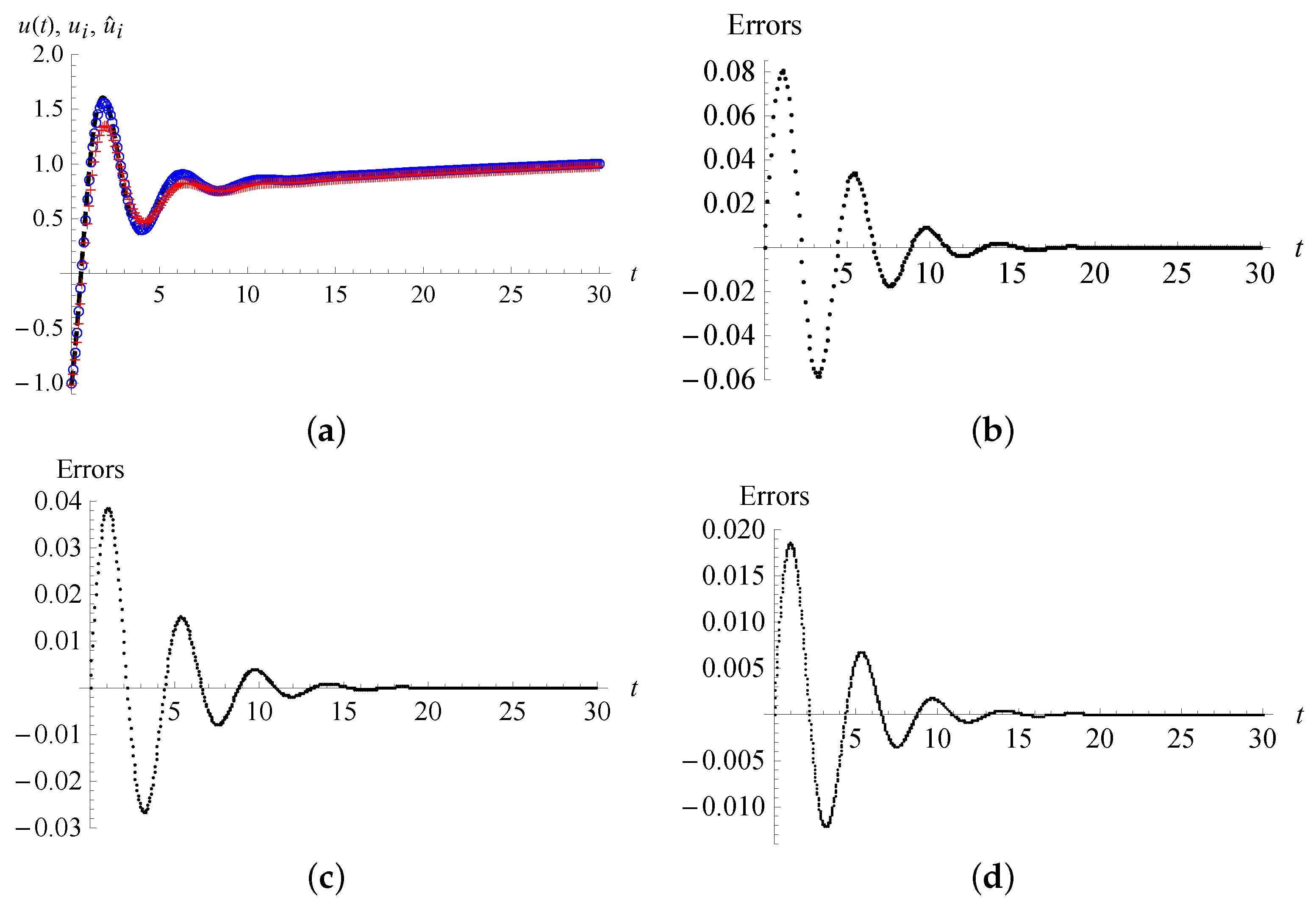
u ( t ) = u 0 E α , 1 2 t α + m 0 t E α , 2 2 t α + Γ ( 1.2 ) t α + 0.2 E α , α + 1.2 2 t α .
We take α = 1.7 , u 0 = 1 , m 0 = 1 to compute the quadratic spline numerical solutions u i on the interval [ 0 , 30 ] from Equation (27) and compare them with the exact solution in Equation (31) and the L 1 L 2 numerical solutions u ^ i . In Figure 1a, the black dash line is depicted from the exact solution in Equation (31), while the blue circles denote the numerical solutions u i and the red crosses denote the numerical solutions u ^ i by using h = 0.1 . In Figure 1b–d, the errors u ( t i ) u i of the numerical solutions u i are plotted for the different step-sizes h = 0.1, 0.05 and 0.025, respectively.
We examined the numerical solutions u ^ i derived from the L 1 L 2 methods with the same step-sizes and found that the errors also decrease oscillatorily as t increases, but the maximal error is about five times of that of the numerical solutions u i . For example, in Figure 2, we depict the plot of the errors u ( t i ) u ^ i of the numerical solutions u ^ i derived from the L 1 L 2 methods with the step-size h = 0.05 on the interval 0 t 30 . Compared with the errors of the numerical solutions u i with the identical step-size in Figure 1c, the maximal errors of the numerical solutions u ^ i increases to about five times.
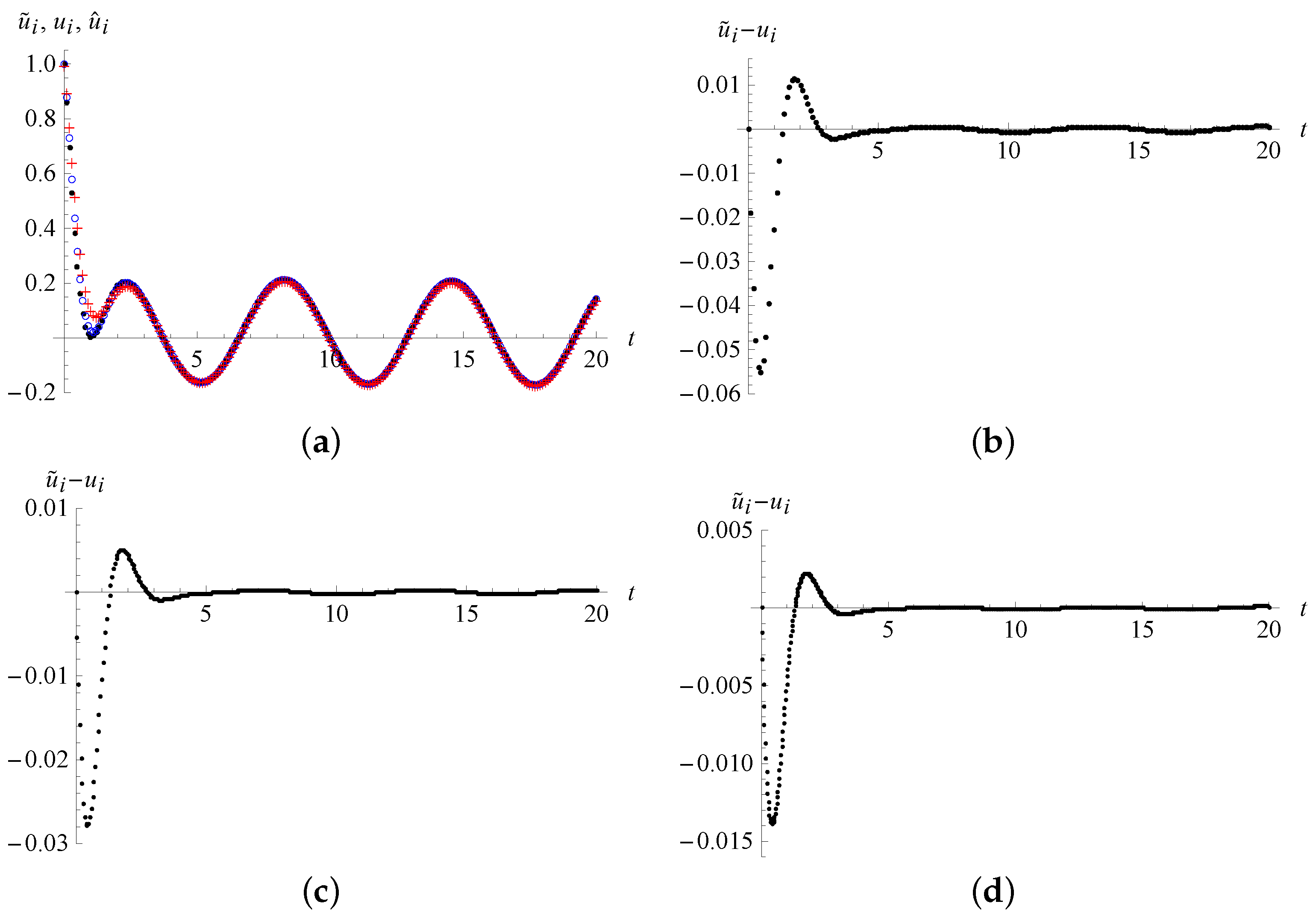
Example 2.
Consider the initial value problem for the fractional differential equation
D t 1.7 u ( t ) + u ( t ) + D t 0.5 u ( t ) + 5 u ( t ) = sin ( t ) , u ( 0 ) = 1 , u ( 0 ) = 1 .
For this example, we use the high-precision numerical inverse of the Laplace transform proposed by Wang et al. [29] as a reference to the exact solution. The Laplace transform of the solution u ( t ) is
U ( s ) = s 0.7 s 0.3 + 1 + s 0.5 s 1.7 + s + s 0.5 + 5 + 1 ( s 1.7 + s + s 0.5 + 5 ) ( s 2 + 1 ) .
The numerical solutions obtained by the high-precision numerical Laplace inverse transform are denoted by u ˜ i .
In Figure 3a, the three numerical solutions on the interval [ 0 , 20 ] with the step-size h = 0.1 obtained from the high-precision numerical Laplace inverse transform, the present quadratic spline interpolation and the L 1 L 2 methods are displayed. In the initial stage, we can readily see that the quadratic spline numerical solutions u i are closer to u ˜ i than the L 1 L 2 numerical solutions.
The differences of the two numerical solutions u ˜ i and u i are shown in Figure 3b–d for h = 0.1 , 0.05 and 0.025, respectively. We also examined the differences of the numerical solutions u ˜ i and u ^ i and found that for a same step-size, the maximum value of | u ˜ i u ^ i | is about three times of that of
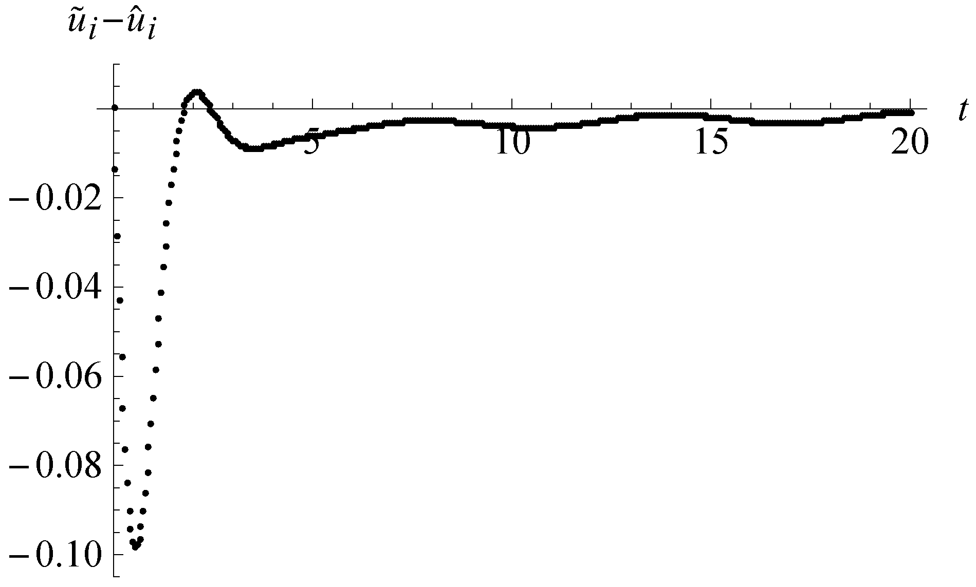
 | u ˜ i u i | . In Figure 4, the differences u ˜ i u ^ i of the numerical solutions from the high-precision inverse Laplace transform and the L 1 L 2 methods with the step-size h = 0.05 are shown. Compared with Figure 3c, the maximum value in Figure 4 enlarges to about three times.
The considered equation belongs to the forced fractional oscillation equation. In Example 1, the transient oscillation evolves into steady-state increasing, while in Example 2, the transient oscillation grows into steady-state oscillation. Two examples show that the decreasing of the step-size h can effectively enhance the accuracy of the numerical solutions, and the present quadratic spline numerical solutions have higher precision than the L 1 L 2 numerical solutions. It is worth noting that for the considered problem, in the initial stage the numerical solutions emerge slightly large errors, but with the process evolution errors can fall off in an oscillatory manner. In Example 1, the second-order derivative of the exact solution u ( t ) does not exist at t = 0 . This responds the unusual errors in the initial stage.
We note that if a differentiable nonlinearity g ( u ( t ) ) is added in the left hand side of Equation (2), then we can approximate the nonlinearity at t = t i , i 1 , as g ( u ( t i ) ) g ( u ( t i 1 ) ) + g ( u ( t i 1 ) ) u ( t i 1 ) h to derive an explicit scheme of numerical solutions in the nonlinear case. Inasmuch as we focus on the numerical schemes for the fractional derivatives by using the quadratic splines, examples in the nonlinear case are not involved.

5. Conclusions

We considered numerical solutions of a fractional differential equation with two Caputo fractional derivative terms, D t α u ( t ) , 1 < α < 2 , and D t β u ( t ) , 0 < β < 1 . The proposed numerical algorithm is based on the method of quadratic spline interpolation. First, we derived discrete expressions of the two fractional derivatives at nodes based on the quadratic spline interpolation function. Then, the recursion scheme for numerical solutions was generated and the approximate solution in the form of quadratic spline function was obtained. Additionally, error estimations were considered. Two numerical examples were used to check the proposed method. For the considered fractional differential equation with the leading order α between 1 and 2, the involved undetermined parameters in the quadratic spline interpolation function can be exactly resolved.
Compared with the L 1 L 2 numerical solutions, where the first two node values need to be given, the iterative scheme of the present quadratic spline numerical solutions only needs to know the value of the first node u 0 , i.e., the iterative scheme starts from u 1 . An improved accuracy is shown in the two examples. The results give the discrete numerical solutions, and the continuous solution with continuous derivative composed of piecewise quadratic polynomials.

Author Contributions

Conceptualization, J.-S.D. and M.L.; data curation, Y.W. and Y.-L.A.; formal analysis, J.-S.D., M.L., Y.W. and Y.-L.A.; funding acquisition, J.-S.D., M.L. and Y.-L.A.; investigation, J.-S.D. and M.L.; methodology, J.-S.D., M.L., Y.W. and Y.-L.A.; software, Y.W. and Y.-L.A.; supervision, J.-S.D. and M.L.; validation, M.L.; visualization, Y.W. and Y.-L.A.; writing—original draft, J.-S.D., M.L. and Y.W.; writing—review and editing, J.-S.D., M.L., Y.W. and Y.-L.A. All authors have read and agreed to the published version of the manuscript.

Funding

This work was supported by the National Natural Science Foundation of China (Nos. 61672238, 12071302 and 11772203).

Institutional Review Board Statement

Not applicable.

Informed Consent Statement

Not applicable.

Data Availability Statement

Not applicable.

Conflicts of Interest

The authors declare no conflict of interest.

References

  1. Oldham, K.B.; Spanier, J. The Fractional Calculus; Academic: New York, NY, USA, 1974. [Google Scholar]
  2. Miller, K.S.; Ross, B. An Introduction to the Fractional Calculus and Fractional Differential Equations; Wiley: New York, NY, USA, 1993. [Google Scholar]
  3. Podlubny, I. Fractional Differential Equations; Academic: San Diego, CA, USA, 1999. [Google Scholar]
  4. Kilbas, A.A.; Srivastava, H.M.; Trujillo, J.J. Theory and Applications of Fractional Differential Equations; Elsevier: Amsterdam, The Netherlands, 2006. [Google Scholar]
  5. Mainardi, F. Fractional Calculus and Waves in Linear Viscoelasticity; Imperial College: London, UK, 2010. [Google Scholar]
  6. Diethelm, K. The Analysis of Fractional Differential Equations; Springer: Berlin, Germany, 2010. [Google Scholar]
  7. Monje, C.A.; Chen, Y.Q.; Vinagre, B.M.; Xue, D.; Feliu, V. Fractional-Order Systems and Controls, Fundamentals and Applications; Springer: Berlin, Germany, 2010. [Google Scholar]
  8. Li, M. Theory of Fractional Engineering Vibrations; De Gruyter: Berlin, Germany; Boston, MA, USA, 2021. [Google Scholar]
  9. Wu, G.C.; Baleanu, D.; Xie, H.P.; Chen, F.L. Chaos synchronization of fractional chaotic maps based on the stability condition. Physica A 2016, 460, 374–383. [Google Scholar] [CrossRef]
  10. Cao, W.; Xu, Y.; Zheng, Z. Existence results for a class of generalized fractional boundary value problems. Adv. Differ. Equ. 2017, 2017, 348. [Google Scholar] [CrossRef]
  11. Băleanu, D.; Diethelm, K.; Scalas, E.; Trujillo, J.J. Fractional Calculus Models and Numerical Methods; Series on Complexity, Nonlinearity and Chaos; World Scientific: Boston, MA, USA, 2012. [Google Scholar]
  12. Li, C.; Zeng, F. Numerical Methods for Fractional Calculus; CRC Press: Boca Raton, FL, USA, 2015. [Google Scholar]
  13. Hajipour, M.; Jajarmi, A.; Baleanu, D. An efficient nonstandard finite difference scheme for a class of fractional chaotic systems. J. Comput. Nonlinear Dynam. 2018, 13, 021013. [Google Scholar] [CrossRef]
  14. Baleanu, D.; Inc, M.; Yusuf, A.; Aliyu, A.I. Space-time fractional Rosenou-Haynam equation: Lie symmetry analysis, explicit solutions and conservation laws. Adv. Differ. Equ. 2018, 2018, 46. [Google Scholar] [CrossRef] [Green Version]
  15. Liu, F.; Zhuang, P.; Anh, V.; Turner, I.; Burrage, K. Stability and convergence of the difference methods for the space-time fractional advection-diffusion equation. Appl. Math. Comput. 2007, 191, 12–20. [Google Scholar] [CrossRef]
  16. Podlubny, I. Matrix approach to discrete fractional calculus. Fract. Calc. Appl. Anal. 2000, 3, 359–386. [Google Scholar]
  17. Li, C.; Wang, Z. The local discontinuous Galerkin finite element methods for Caputo-type partial differential equations: Numerical analysis. Appl. Numer. Math. 2019, 140, 1–22. [Google Scholar] [CrossRef]
  18. Liu, L.; Xue, D.; Zhang, S. Closed-loop time response analysis of irrational fractional-order systems with numerical Laplace transform technique. Appl. Math. Comput. 2019, 350, 133–152. [Google Scholar] [CrossRef]
  19. Jafari, H.; Khalique, C.M.; Ramezani, M.; Tajadodi, H. Numerical solution of fractional differential equations by using fractional B-spline. Cent. Eur. J. Phys. 2013, 11, 1372–1376. [Google Scholar] [CrossRef] [Green Version]
  20. Luo, W.H.; Huang, T.Z.; Wu, G.C.; Gu, X.M. Quadratic spline collocation method for the time fractional subdiffusion equation. Appl. Math. Comput. 2016, 276, 252–265. [Google Scholar] [CrossRef]
  21. Qin, Y.; Wu, K. Numerical solution of fractional bioheat equation by quadratic spline collocation method. J. Nonlinear Sci. Appl. 2016, 9, 5061–5072. [Google Scholar] [CrossRef]
  22. Diethelm, K.; Ford, N.J.; Freed, A.D. A predictor-corrector approach for the numerical solution of fractional differential equations. Nonlinear Dynam. 2002, 29, 3–22. [Google Scholar] [CrossRef]
  23. Gao, G.H.; Sun, Z.Z.; Zhang, H.W. A new fractional numerical differentiation formula to approximate the Caputo fractional derivative and its applications. J. Comput. Phys. 2014, 259, 33–50. [Google Scholar] [CrossRef]
  24. Garrappa, R. Numerical solution of fractional differential equations: A survey and a software tutorial. Mathematics 2018, 6, 16. [Google Scholar] [CrossRef] [Green Version]
  25. Wang, T.; Qin, M.; Lian, H. The asymptotic approximations to linear weakly singular Volterra integral equations via Laplace transform. Numer. Algorithms 2020, 85, 683–711. [Google Scholar] [CrossRef]
  26. Li, Y.S. Splines and Interpolations; Science and Technology Press: Shanghai, China, 1983. [Google Scholar]
  27. Xie, S. Quadratic and cubic spline interpolation. J. Approx. Theory 1984, 41, 21–28. [Google Scholar] [CrossRef]
  28. Li, Y.S.; Huang, Y.Q. Numerical Approximation; People’s Education Press: Beijing, China, 1978. [Google Scholar]
  29. Wang, T.; Gu, Y.; Zhang, Z. An algorithm for the inversion of Laplace transforms using Puiseux expansions. Numer. Algorithms 2018, 78, 107–132. [Google Scholar] [CrossRef]
Figure 1. The exact solution u ( t ) , numerical solutions u i and u ^ i , and the errors of u i in Example 1. (a) The exact solution u ( t ) (dash line), the quadratic spline numerical solutions u i (circles) and the L 1 L 2 numerical solutions u ^ i (crosses) with h = 0.1; (b) the errors of u i (h = 0.1); (c) the errors of u i (h = 0.05); (d) the errors of u i (h = 0.025).
Fractalfract 06 00369 g001
Figure 2. The errors of the L 1 L 2 numerical solutions u ^ i ( h = 0.05 ).
Fractalfract 06 00369 g002
Figure 3. The numerical solutions and comparisons in Example 2. (a) The numerical solutions with h = 0.1 by the inverse Laplace transform, u ˜ i (dots), the quadratic spline interpolation u i (circles) and the L 1 L 2 methods u ^ i (crosses); (b) the differences of the two numerical solutions u ˜ i and u i (h = 0.1); (c) the differences of the two numerical solutions u ˜ i and u i (h = 0.05); (d) the differences of the two numerical solutions u ˜ i and u i (h = 0.025).
Fractalfract 06 00369 g003
Figure 4. The difference u ˜ i u ^ i between the high-precision inverse Laplace transform numerical solutions and the L 1 L 2 numerical solutions ( h = 0.05 ).
Fractalfract 06 00369 g004
Publisher’s Note: MDPI stays neutral with regard to jurisdictional claims in published maps and institutional affiliations.

