Article

Particle Swarm Optimization Fractional Slope Entropy: A New Time Series Complexity Indicator for Bearing Fault Diagnosis

1
School of Automation and Information Engineering, Xi’an University of Technology, Xi’an 710048, China
2
Shaanxi Key Laboratory of Complex System Control and Intelligent Information Processing, Xi’an University of Technology, Xi’an 710048, China
*
Author to whom correspondence should be addressed.
Fractal Fract. 2022, 6(7), 345; https://doi.org/10.3390/fractalfract6070345
Submission received: 5 June 2022 / Revised: 19 June 2022 / Accepted: 20 June 2022 / Published: 21 June 2022

Abstract

:
Slope entropy (SlEn) is a time series complexity indicator proposed in recent years, which has shown excellent performance in the fields of medical and hydroacoustics. In order to improve the ability of SlEn to distinguish different types of signals and solve the problem of two threshold parameters selection, a new time series complexity indicator on the basis of SlEn is proposed by introducing fractional calculus and combining particle swarm optimization (PSO), named PSO fractional SlEn (PSO-FrSlEn). Then we apply PSO-FrSlEn to the field of fault diagnosis and propose a single feature extraction method and a double feature extraction method for rolling bearing fault based on PSO-FrSlEn. The experimental results illustrated that only PSO-FrSlEn can classify 10 kinds of bearing signals with 100% classification accuracy by using double features, which is at least 4% higher than the classification accuracies of the other four fractional entropies.

1. Introduction

Entropy is a measure of the complexity of time series [1,2,3,4,5], among which the entropies based on Shannon entropy [6] are the most widely used, including permutation entropy (PE) [7], dispersion entropy (DE) [8], etc. The definition of PE is based on the sequential relationship among the time series. Moreover, the concept of PE is simple, and its calculation speed is fast [9], but its stability is not very good. Therefore, as an improved algorithm of PE, dispersion entropy (DE) is proposed, which has the advantages of little influence by burst signals and good stability [10]. These two kinds of entropies and their improved entropies have shown good results in various fields [11,12,13].
PE is one of the most commonly used time series complexity estimators. PE has clearly proved its usefulness in mechanical engineering, mainly in the field of fault diagnosis. Taking the research on fault diagnosis for rolling bearing as an example, the advantage of PE is that it is not limited by the bearing signals and the length of permutation samples [14]. However, PE does not take the difference between the amplitude values. In order to consider the amplitude information of time series, the complexity of time series is analyzed by weighted permutation entropy (WPE) [15]. It is concluded that WPE not only has the same advantages as PE, but also can detect the complexity of dynamic mutation by quantifying amplitude information. Concurrently, other application fields of PE and WPE have also received great attention [16,17,18,19].
As an improved algorithm of PE, DE also introduces amplitude information, and has the advantage of distinguishing different types of signals easily and calculating fast. Regarding the applications of DE, it has been used widely in bearing signals classification. In the feature extraction experiment of bearing fault diagnosis, DE can classify bearing faults through short data, and has high recognition accuracy in the case of small samples [20]. However, DE is impossible to evaluate the fluctuation of time series. Thus, the fluctuation information is combined with DE to obtain fluctuating dispersion entropy (FDE) [21]. FDE takes into account the fluctuation of time series, which can discriminate deterministic from stochastic time series. And relative to DE, FDE reduces all possible dispersion modes to speed up the calculation of entropy. After that, DE and FDE have also made great achievements in the fields of medicine and underwater acoustics [22,23]. In order to make the feature of DE more significant, fractional calculus is proposed to combine with DE [24], where fractional calculus can introduce fractional information into entropy [25]. Similarly, there is the existence of fractional fuzzy entropy (FE), which is the combination of fractional calculus and FE [26].
Slope entropy (SlEn) is a new time series complexity estimator proposed in recent years. Its concept is simple, which is only based on the amplitude of time series and five modules. Since it was proposed, it has been used in the fields of medical, hydroacoustics, and fault diagnosis. In 2019, SlEn was first proposed by David Cuesta-Frau, and successively applied it to the classification of electroencephalographic (EEG) records and electromyogram (EMG) records [27], classify the activity records of patients with bipolar disorder [28], and the features extraction of fever time series [29]. Then SlEn is also used to extract the features of ship radiated noise signals [30] and bearing fault signals [31].
SlEn has proven to have strong superiority as features. However, SlEn has not received the attention it deserves. A big factor that leads to this situation is the influence of the two threshold parameter settings on its effect. Therefore, in order to solve this problem, we introduce particle swarm optimization (PSO) algorithm to optimize these two threshold parameters. Another factor is that there is still room for improvement in the basic SlEn. Therefore, in order to improve the significance of features, we combine fractional calculus with SlEn. Finally, a new algorithm named PSO fractional SlEn (PSO-FrSlEn) is proposed in this paper, which is an improved time series complexity indicator of SlEn.
The structure of this paper is divided as follows. Section 2 introduces the algorithm steps of the proposed method in detail. Section 3 exhibits the experimental process of this paper briefly. Section 4 and Section 5 demonstrate the experiment and analysis of single feature extraction and double feature extraction separately. Finally, the innovations of this paper and the conclusions of the experiments are drawn in Section 6.

2. Algorithms

2.1. Slope Entropy Algorithm

For a given time series S = { s i ,   i = 1 ,   2 ,   3 ,   ,   n } , SlEn is calculated according to the following steps.
Step 1:
set an embedding dimension m, which can divide the time series into k = n m + 1 subsequences, where m is greater than two and much less than n . The disintegrate form is as follows:
S k = { s k ,   s k + 1 ,   ,   s n }
Here, all subsequences S 1 ,   S 2 ,   , S k contain m elements, such as S 1 = { s 1 ,   s 2 ,   ,   s m } .
Step 2:
subtract the latter of the two adjacent elements in all the subsequences obtained in Step 1 from the former to obtain k new sequences. The new form is as follows:
T k = { t k ,   t k + 1 ,   ,   t n 1 }
Here, the element t k = s k + 1 s k , and all sequences T 1 ,   T 2 ,   , T k contain m 1 elements, such as T 1 = { t 1 ,   t 2 ,   ,   t m 1 } .
Step 3:
lead into the two threshold parameters η and ε of SlEn, where 0 < ε < η , and compare all elements in the sequences obtained from Step 2 with the positive and negative values of these two threshold parameters. The positive and negative values of these two threshold parameters η , ε ,   ε and η serve as the dividing lines, they divide the number field into five modules 2 , 1 ,   0 ,   1 , and 2 . If t k < η , the module is 2 ; if η < t k < ε , the module is 1 ; if ε < t k < ε , the module is 0 ; if ε < t k < η , the module is 1 ; if ε < t k < ε , the module is 0 ; if t k > η , the module is 2 . The intuitive module division principle is shown by the coordinate axis in Figure 1 below:
The form of the sequences is below:
E k = { e k ,   e k + 1 ,   ,   e n 1 }
Here, each element in E k is 2, 1, 0, 1, or 2, and there will be the exactly the same sequence.
Step 4:
the number of modules is 5, so all types of the sequences E k are counted as j = 5 m 1 . Such as when m is 3, there will be at most 25 types of E k , which are { 2 , 2 } , { 2 , 1 } , …, { 0 ,   0 } , { 0 ,   1 } , …, { 2 ,   1 } , { 2 ,   2 } . The number of each type records as r 1 ,   r 2 ,   ,   r j , and the frequency of each type is calculated as follows:
R j = r j k
Step 5:
based on the classical Shannon entropy, the formula of SlEn is defined as follows:
S l o p e E n ( m ,   η ,   ε ) = j R j ln R j

2.2. Fractional Slope Entropy Algorithm

In this paper, the concept of fractional order is introduced into SlEn for the first time, and the calculation formula of the improved algorithm of SlEn (FrSlEn) is obtained through the following steps.
Step 1:
Shannon entropy is the first entropy to consider fractional calculus, and its generalized expression is as follows:
S h a n n o n E n α = j p i { p i α Γ ( α + 1 ) [ ln p i + ψ ( 1 ) ψ ( 1 α ) ] }
Here, α is the order of fractional derivative, Γ   ( · ) and ψ   ( · ) are the gamma and digamma functions.
Step 2:
extract the fractional order information of order α from Equation (6):
I α = p i α Γ ( α + 1 ) [ ln p i + ψ ( 1 ) ψ ( 1 α ) ]
Step 3:
combine the fractional order with SlEn, which is to replace ln R j with Equation (7). Therefore, the formula of FrSlEn is defined as follows:
S l o p e E n α ( m ,   η ,   ε ) = j R j { R j α Γ ( α + 1 ) [ ln R j + ψ ( 1 ) ψ ( 1 α ) ] }

2.3. Particle Swarm Optimization and Algorithm Process

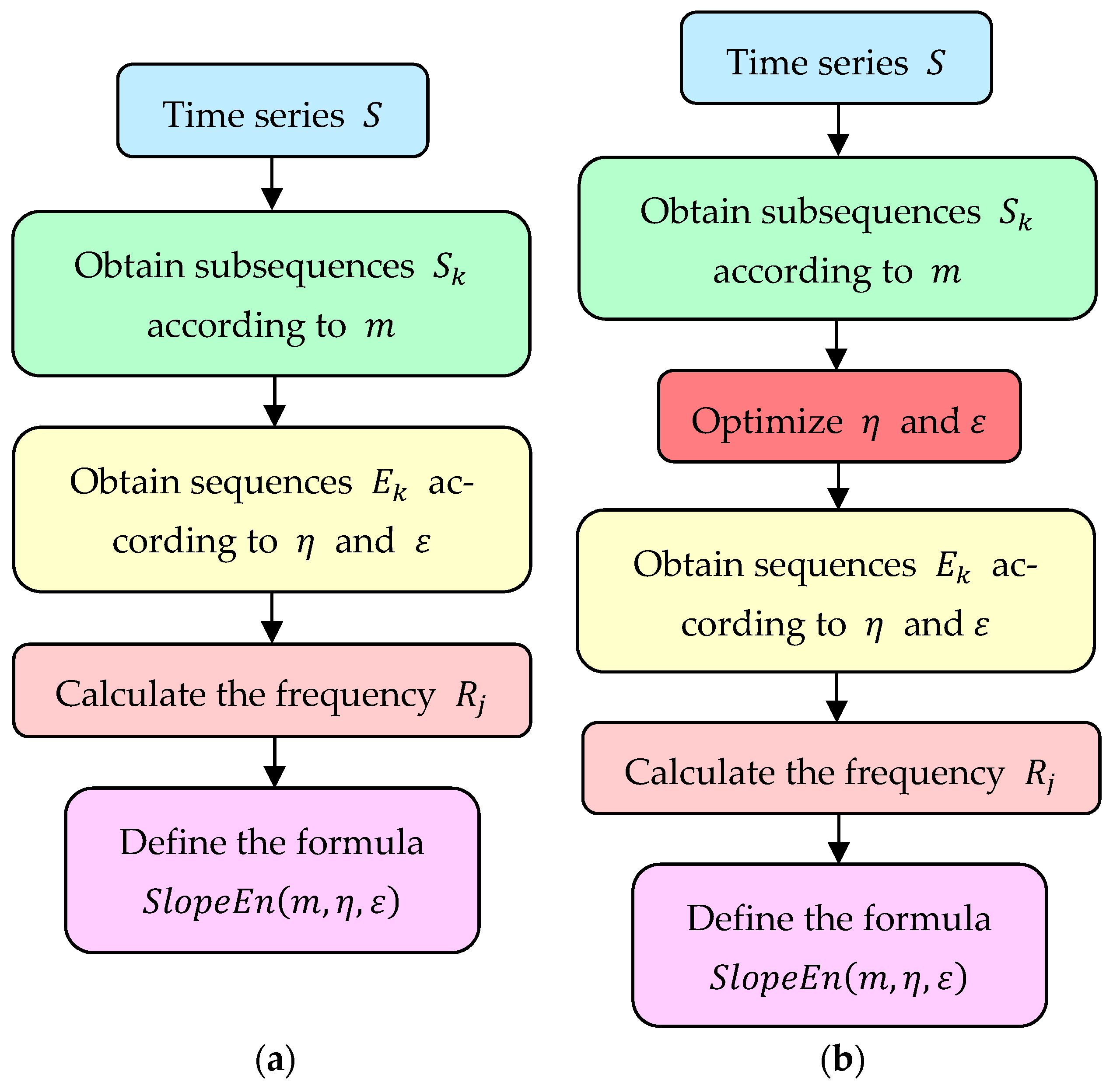
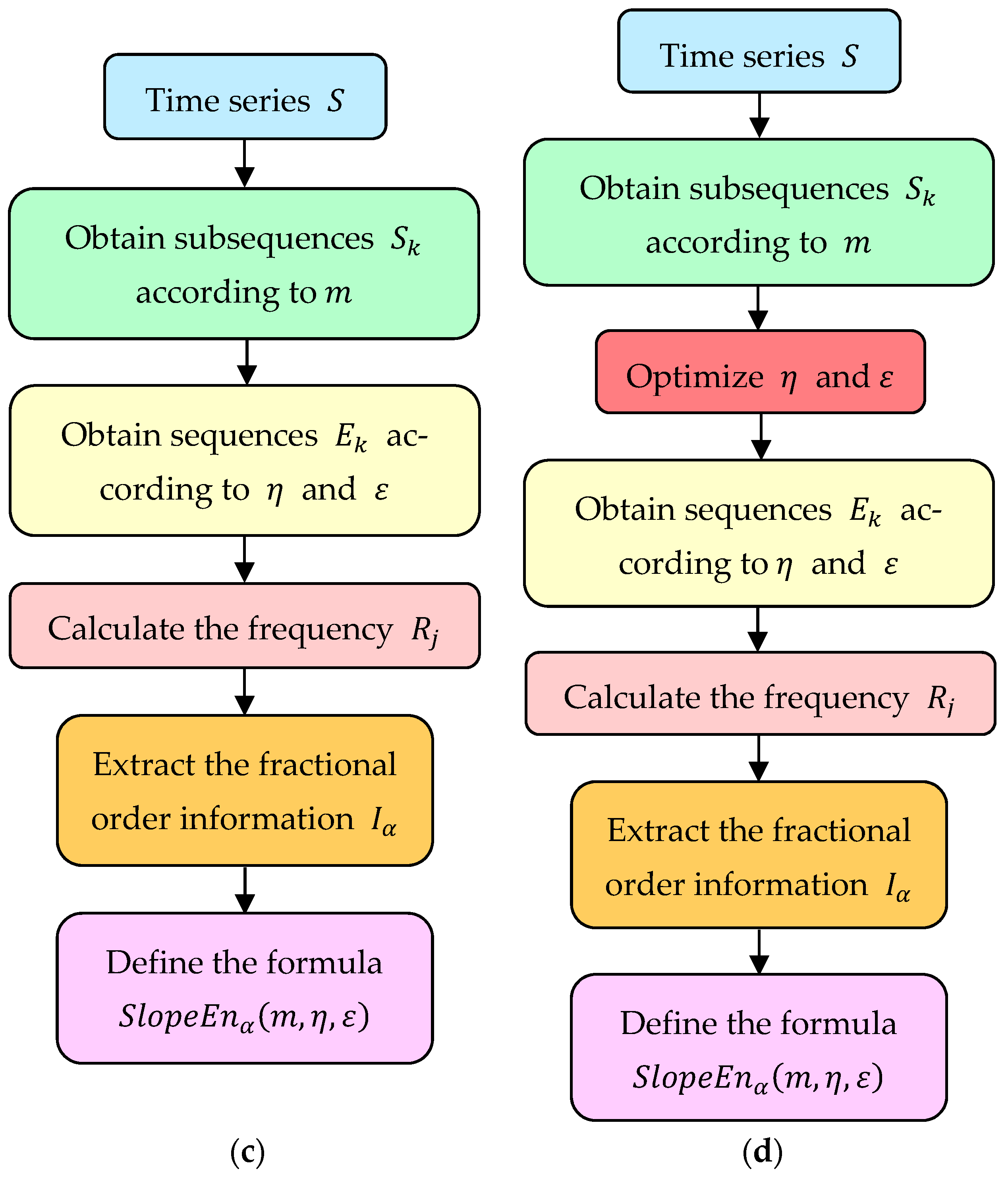
In order to get a better effect of FrSlEn, we use particle swarm optimization (PSO) algorithm to optimize the two threshold parameters η and ε of SlEn. Considering all the above algorithm steps and conditions, the algorithm flowchart of SlEn and three kinds of improved SlEn is as follows in Figure 2:

3. Proposed Feature Extraction Methods

The experiment of this paper is divided into two parts: single feature extraction and double feature extraction. The specific experimental process of single feature extraction is as follows.
Step 1:
the 10 kinds of bearing signals are normalized, which can make the signals neat and regular, the threshold parameters η and ε less than 1, where ε is less than 0.2 in most cases.
Step 2:
the five kinds of single features of these 10 kinds of normalized bearing signals are extracted separately under seven different fractional orders.
Step 3:
the distribution of the features is obtained and the hybrid degrees between the feature points are observed.
Step 4:
these features are classified into one of the 10 bearing signals by K-Nearest Neighbor (KNN).
Step 5:
the classification accuracies of the features are calculated.
The experimental process of double feature extraction is roughly the same as that of single feature extraction. In the Step 2 of double feature extraction, combine any two different fractional orders of the seven fractional orders as double features, which can obtain 21 double feature combinations. The experimental process flowchart is as follows in Figure 3:

4. Single Feature Extraction

4.1. Bearing Signals

The object of this paper is bearing signal. Ten kinds of bearing signals with different faults and fault diameter sizes under the same working state are randomly selected and downloaded for this paper, and the 10 kinds of bearing signals come from the same website [32].
The signal data are measured when the motor load is three horsepower. First of all, it is essential to have a normal bearing signal, which is coded as N-100. Then, the bearing fault signals are divided into three types: inner race fault signals, ball fault signals and outer race fault signals, where for the outer race fault signals, the relative position coincidence area of the outer race is the central direction (six o’clock direction). Finally, there are three kinds of fault diameter sizes, which are 0.007 in, 0.014 in, and 0.021 in. According to the three different types of faults and the three different sizes of fault diameter, the fault signals are divided into nine categories, and they are coded as IR-108, B-121, OR-133, IR-172, B-188, OR-200, IR-212, B-225, and OR-237.
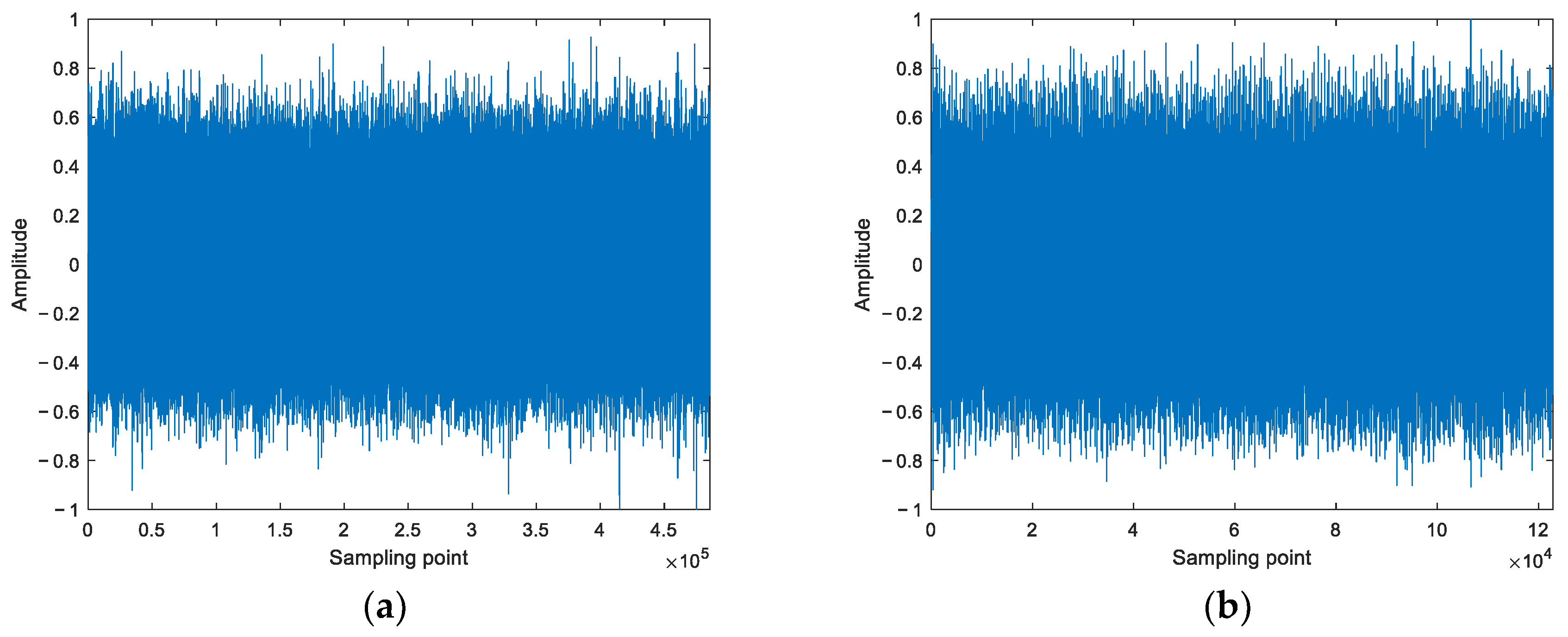
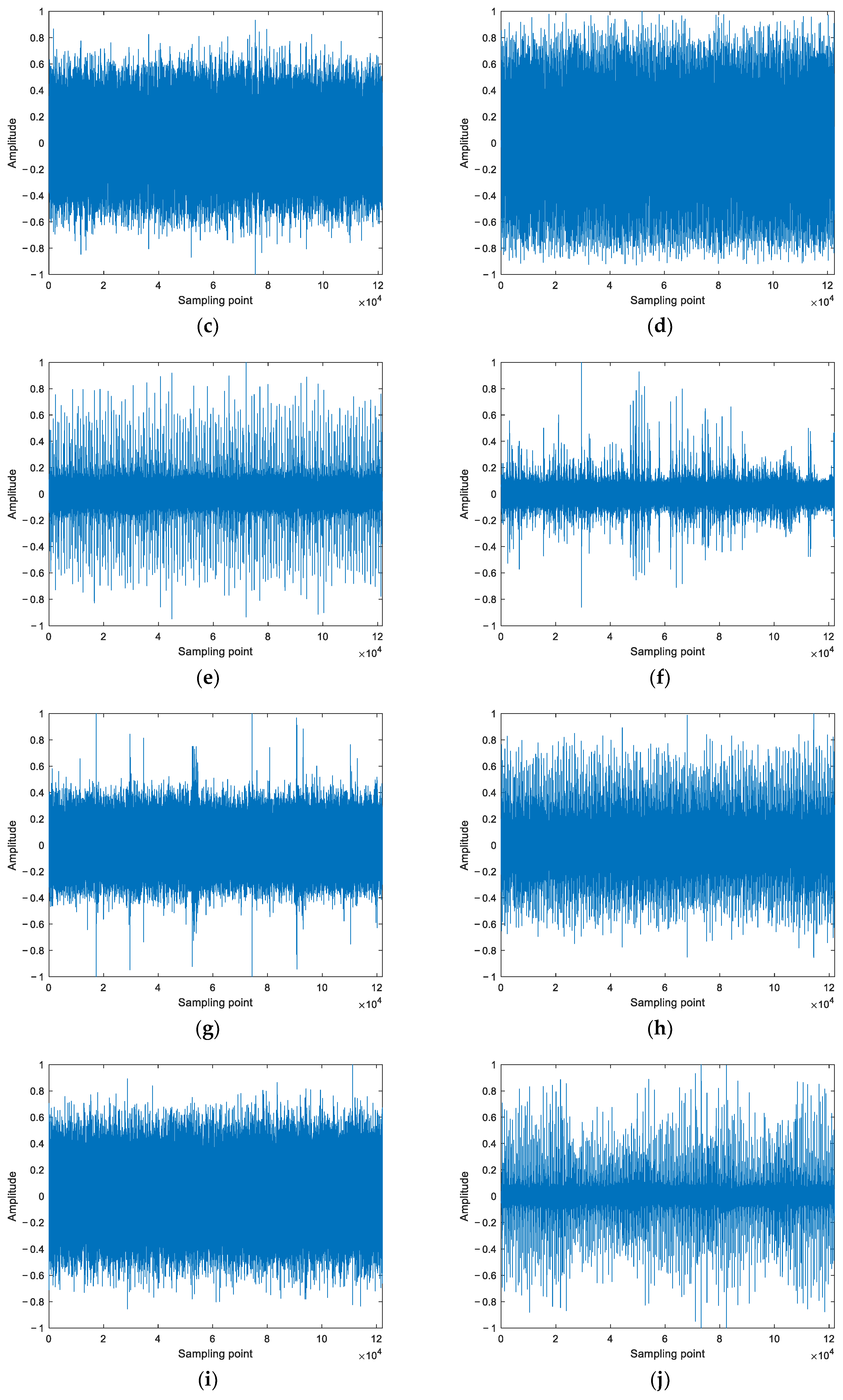
The data files are in MATLAB format, and each file contains the acceleration time series data of drive end, fan end and base. The drive end acceleration time series data are chosen as the experimental data in this paper. The signals data are normalized, and the normalized signals are shown in Figure 4.

4.2. Feature Distribution

In this paper, five kinds of entropies based on Shannon entropy are selected as the features of the above 10 bearing signals for feature extraction. The five kinds of entropies are PE, WPE, DE, FDE, and SlEn, which are renamed FrPE, FrWPE, FrDE, FrFDE, and FrSlEn after combining with the fractional orders.
The parameters shared by different entropies are necessary to be set to the same value. There are three parameters of FrPE and FrWPE, five parameters of FrDE and FrFDE, and four parameters of FrSlEn, where the two same parameters of them are embedding dimension ( m ) and fractional order ( α ). So set all the m as 4, and take all the α from 0.3 to 0.3, where α = 0 is the case without fractional order. The same parameter of FrPE, FrWPE, FrDE, and FrFDE is time lag ( τ ), and all the τ are set as 1. The two proprietary parameters of FrDE and FrFDE are number of classes ( c ) and mapping approach, we set the c of them as 3 and the mapping approach of them is normal cumulative distribution function (NCDF). There are two threshold parameters of FrSlEn are proprietary, which are large threshold ( η ) and small threshold ( ε ). They are non-negative and optimized by PSO in this paper, so FrSlEn is renamed as PSO-FrSlEn.
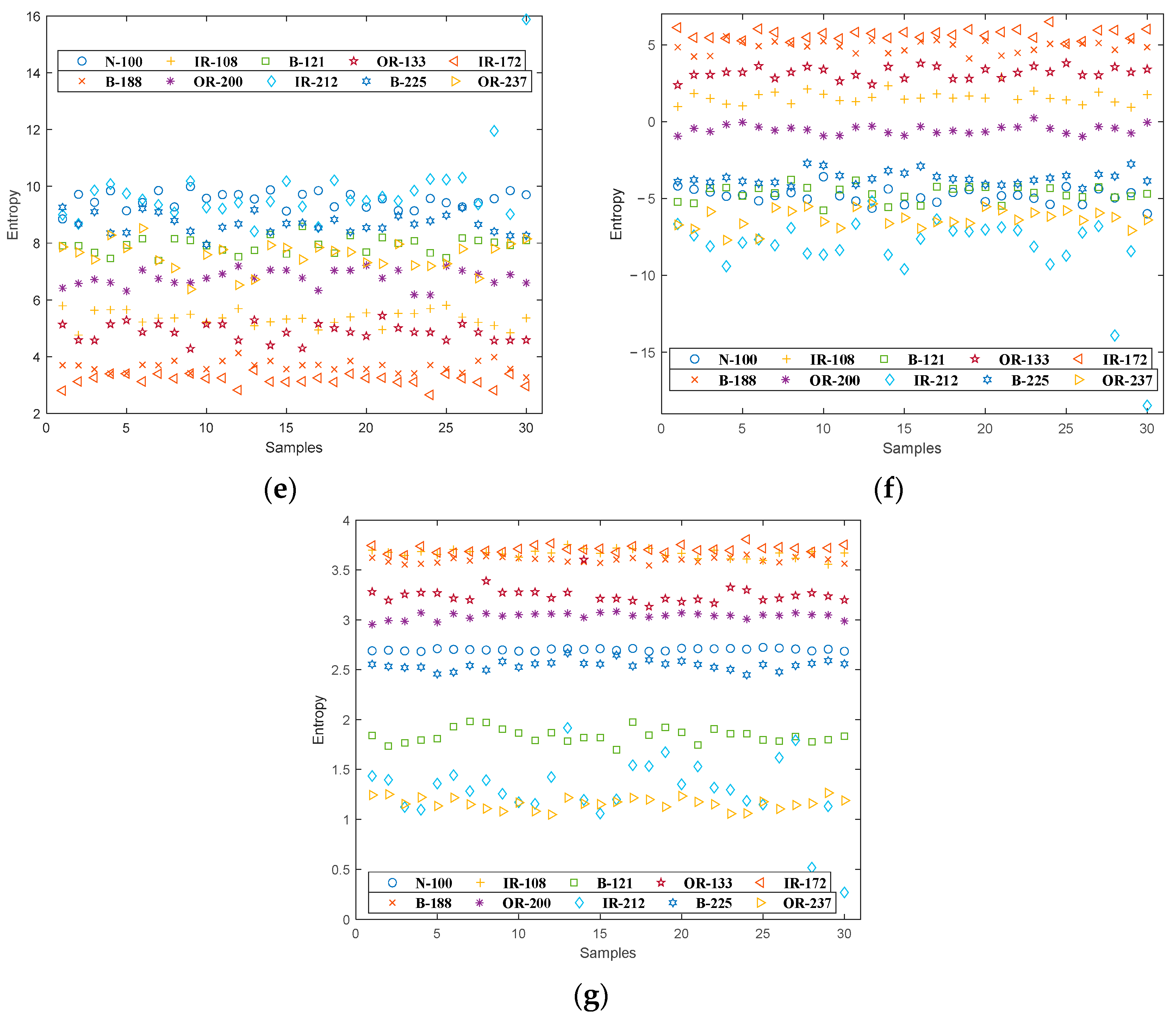
According to the sampling point lengths of the above signals, most of which are just more than 1.2 × 10 5 , every 4000 sample points are taken as one sample, so there are 30 samples for each kind of bearing signals. Combined with all the parameter settings mentioned above, the single features of the 30 samples of each kind of signals are extracted. PSO-FrSlEn under different α is taken as an example, the feature distribution of PSO-FrSlEn is shown in Figure 5 below:
As can be seen from Figure 5, the feature points of B-121, B-225, and OR-237 are obviously mixed under α = 0.3 ; under α = 0.1 , α = 0.2 , and α = 0.3 , the feature points of N-100, B-121, IR-212, B-225, and OR-237 are mixed with each other; all feature points except those of OR-200 are mixed to varying degrees under α = 0.2 and α = 0 ; under α = 0.1 , no kind of feature points is isolated. According to the distribution and confusion degree of these kinds of feature points, we can judge whether each entropy under different α is a notable feature of the signals. In order to intuitively show whether the features are distinguishing, we also undertake classification experiments.

4.3. Classification Effect Verification

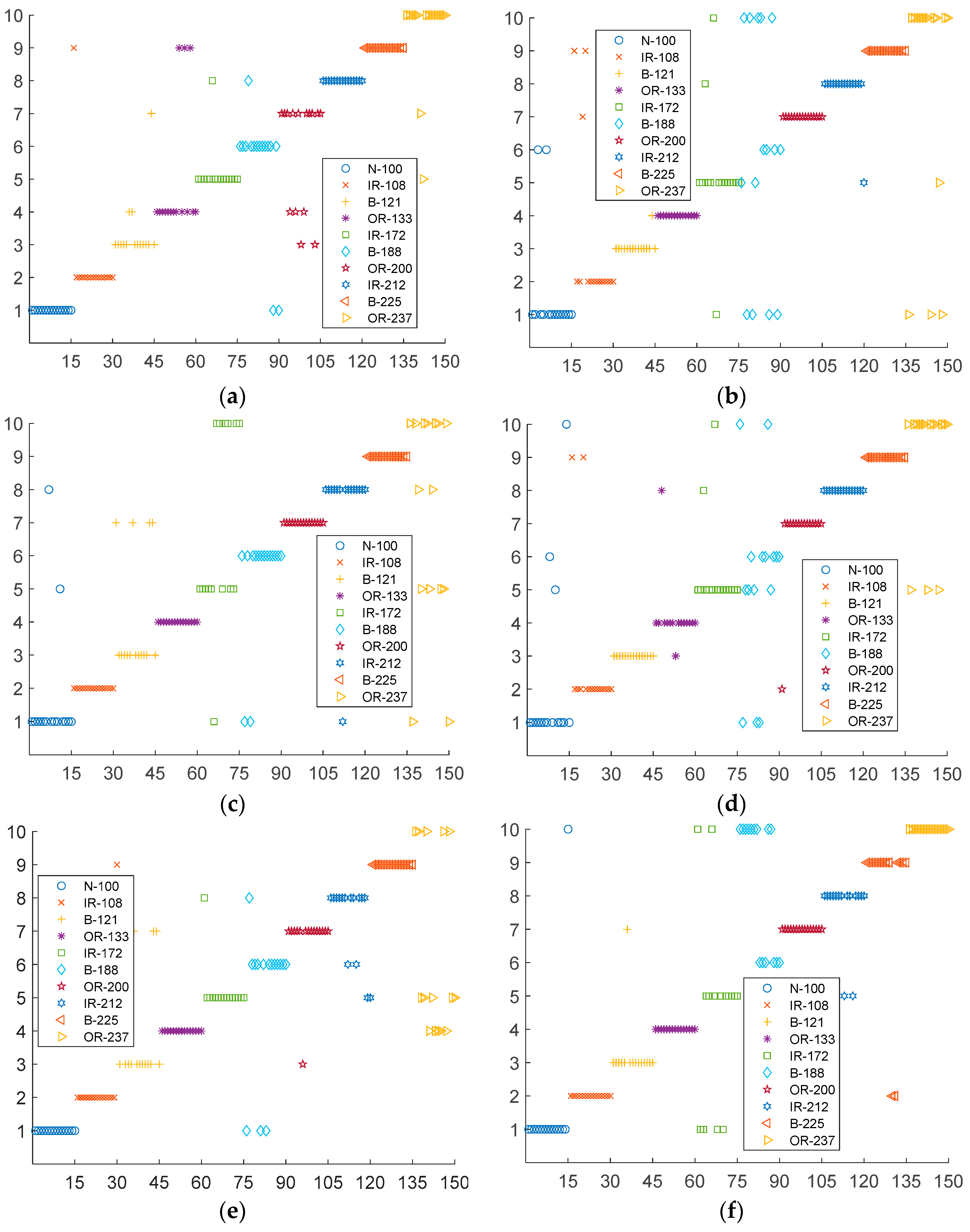
KNN is selected as a classifier for the features, which can classify all the features into the corresponding positions of the signals after being trained. The number of nearest samples k is set as 3 , and 15 samples are taken as training samples and 15 as test samples from the 30 samples of each type of the signals. Also take PSO-FrSlEn as an example. The final classification results and distribution of PSO-FrSlEn are shown in Figure 6 below:
It can be seen from the distribution of sample points in Figure 6, for N-100, IR-108, OR-133, OR-200, IR-212, and B-225, at most five sample points are misclassified; for B-121, more than half of the sample points are misclassified when α = 0 , but at most only four sample points are misclassified when the α is another value, and the classification is completely correct when α = 0.2 ; for IR-172, most of the sample points are misclassified when α = 0.2 and α = 0.1 , but the classification is basically correct when the α is another value; for B-188, the classification effect of sample points is very poor no matter what value α takes except when α = 0.2 ; for OR-237, all sample points can be classified correctly when α = 0.1 . It can be concluded that the classification ability of the same entropy is different under different values of α .
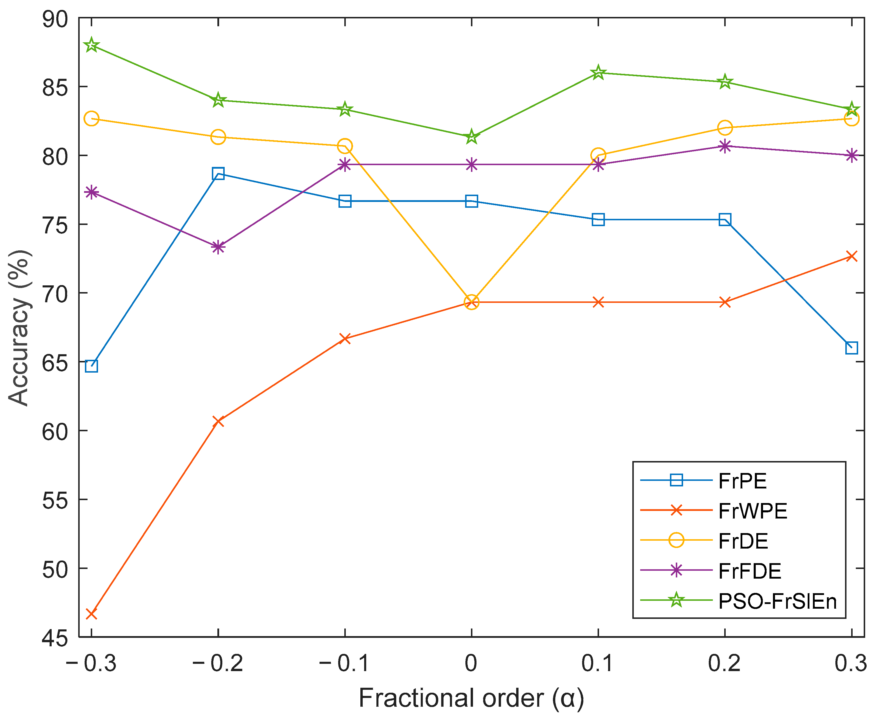
The classification accuracies of each entropy under different fractional orders are obtained after calculation. All the accuracies obtained are recorded in the Table 1 below, and a line graph is drawn in Figure 7 for comparison.
The following information can be obtained from Table 1 and Figure 7, all the classification accuracies are less than 90%; the classification accuracies of PSO-FrSlEn under any fractional orders are greater than those of other arbitrary entropies, and are greater than 80%; the classification accuracies of DE and SlEn with fractional orders are higher than those without fractional orders, which proves that fractional order can make entropy have higher classification accuracy. In order to further improve the classification accuracy and prove the superiority of PSO-FrSlEn, we add a double feature extraction experiment.

5. Double Feature Extraction

5.1. Feature Distribution

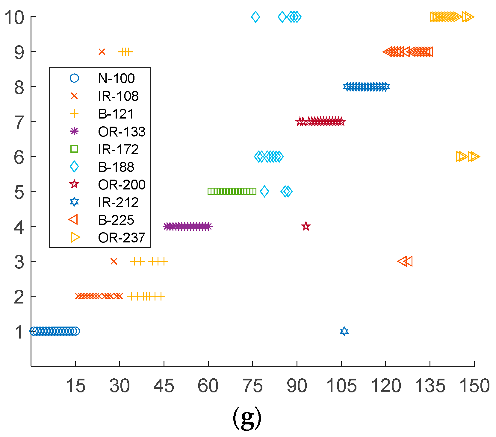
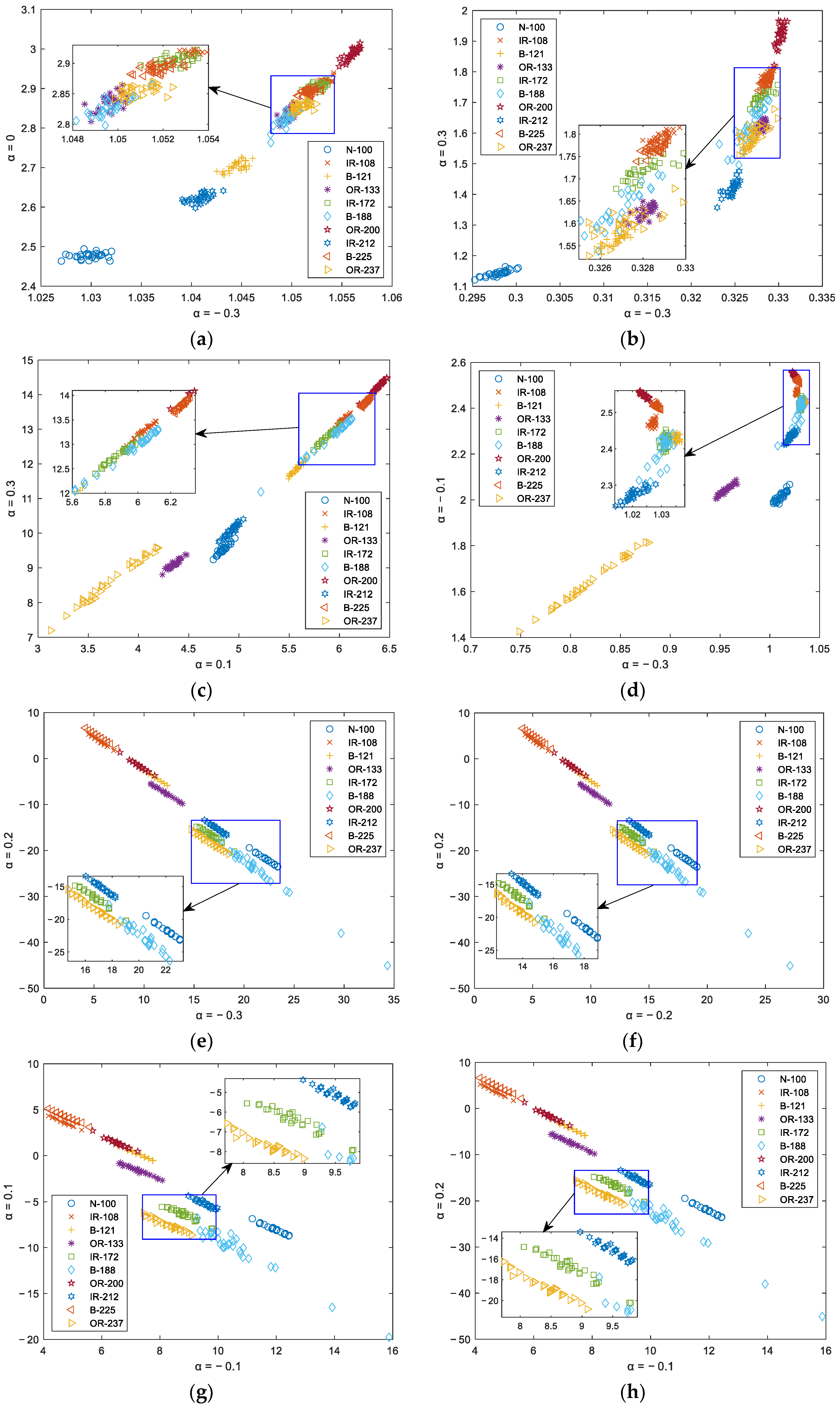
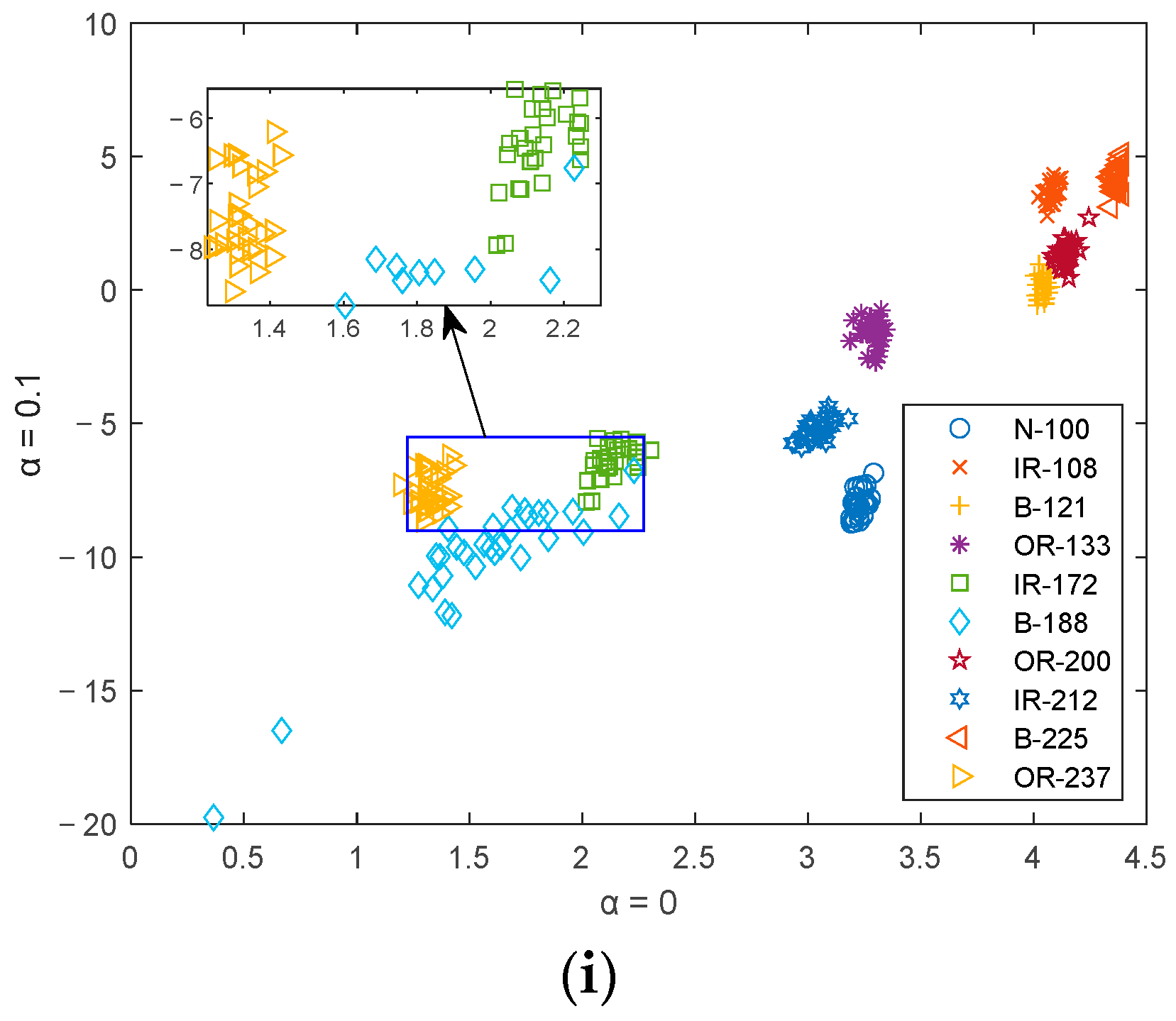
There are 7 values of α , and the classification accuracies of the sample points vary greatly under different α . Therefore, combine any two different α of the same entropy as a fractional order combination. Each entropy can get 21 groups of fractional order combinations. Define the 21 groups of fractional order combinations as 21 double feature combinations, which are 0.3 & 0.2 , 0.3 & 0.1 , 0.3 & 0 ,   ,   0.1 & 0.3 ,   0.2 & 0.3 . There are also 30 samples for each signal in the double feature extraction experiment. Each entropy has 21 double feature combinations, so there are 105 double feature combinations in total. Double feature distribution of the nine highest classification accuracies is shown in Figure 8, in which there is only one highest classification accuracy for FrPE, FrWPE, FrDE, and FrFDE, while there are five highest classification accuracy for PSO-FrSlEn.
We can obtain the following information from Figure 8, for FrPE, most feature points of IR-108, OR-133, IR-172, B-188, B-225, and OR-237 are mixed together; for FrWPE, the feature points of each signal are mixed with each other expect those of N-100, OR-200, and IR-212; for FrDE, only a few feature points of IR-108, IR-172, and B-188 have mixed phenomenon, most feature points of the other signals are connected into lines and parallel to each other; for FrFDE, only the feature points of B-121, IR-172, and B-188 are mixed, but the degree of the mixing is great; for PSO-FrSlEn, only one or two feature points of IR-172 are mixed into the feature points range of B-188, and those of other signals are in their respective own piles and not mixed into the others’ range.
The mixing degree and the kind number of the feature points determine whether these features are significant. The greater the mixing degree of feature points or the more kinds of mixed feature points, the less significant the features are. Therefore, it can be concluded from the above information, the features of FrWPE are the least significant, and those of PSO-FrSlEn are the most significant. In order to confirm this conclusion, we carried out feature classification experiment to verify.

5.2. Classification Effect Verification

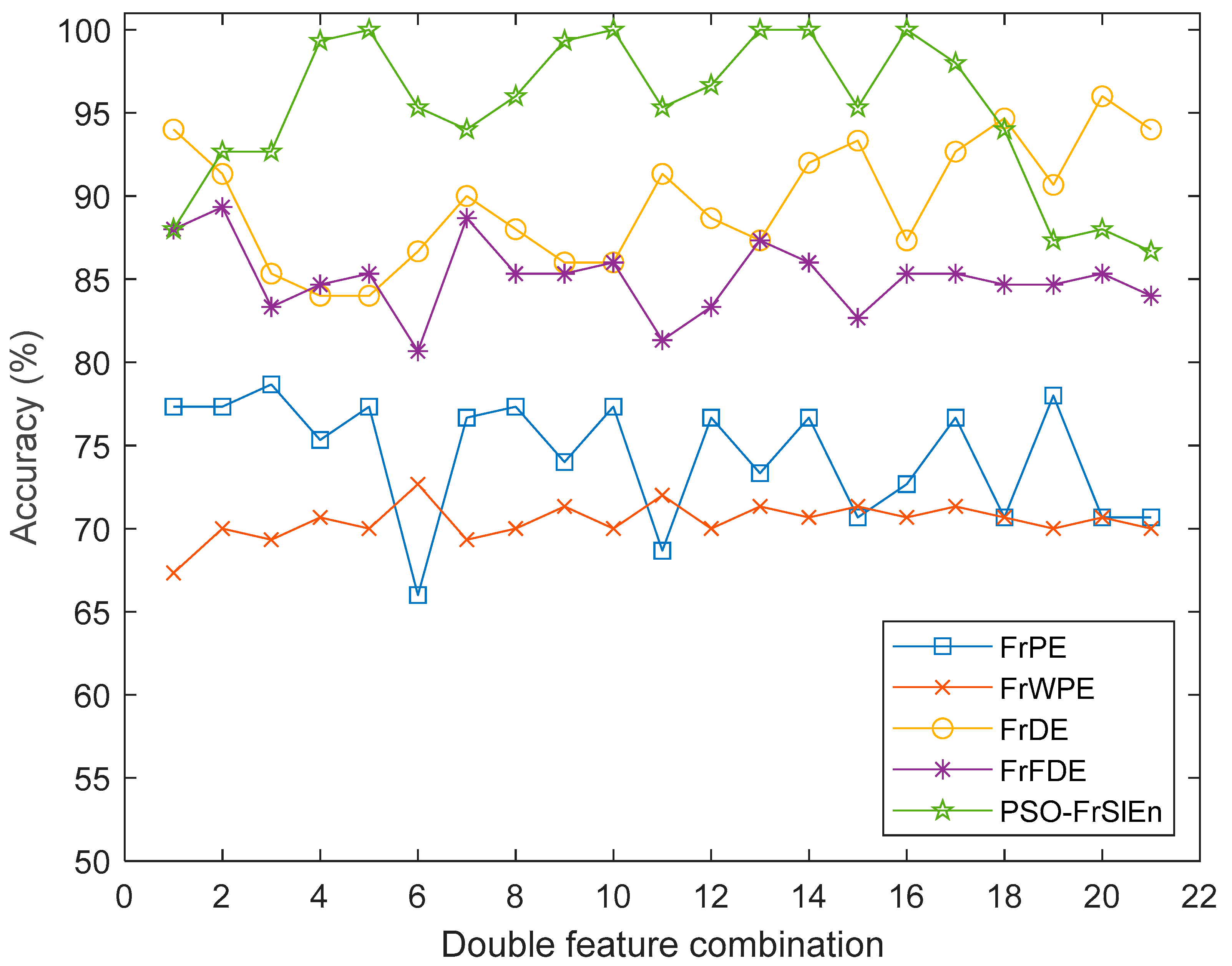
KNN is used as a classifier to classify these double features, and the parameter settings are the same as those in the single feature experiment. The highest classification accuracy of each entropy calculated by the program is shown in Table 2 below. A line graph is drawn in Figure 9 for comparison, where 1 to 21 on the abscissa axis represent the double feature combinations from 0.3   &   0.2 to 0.2   &   0.3 respectively.
As can be seen from the data in Table 2, there are five double feature combinations of PSO-FrSlEn, which can make the feature classification accuracy up to be the highest, and the highest accuracy is 100%; the highest classification accuracy of the other four kinds of entropies is only 96% of FrDE, and the lowest one is 72.67% of FrWPE. The line graph in Figure 9 shows that most double feature combinations of PSO-FrSlEn has higher classification accuracy than the other kinds of entropies. These conclusions are sufficient to prove that the features of PSO-FrSlEn are the most significant to distinguish the 10 kinds of bearing signals.

6. Conclusions

In this paper, the fractional order is combined with the five kinds of entropies, which are PE, WPE, DE, FDE and SlEn, and the features of these five kinds of entropies are extracted for the 10 kinds of bearing signals. Single feature experiment and double feature experiment are carried out respectively. KNN is used to classify these features to verify the significant degree of various features. The main innovations and experimental comparison results are as follows:
(1)
As an algorithm proposed in 2019, SlEn has not been proposed any improved algorithm. It is proposed for the first time to combine the concept of fractional information with SlEn, and get an improved algorithm of SlEn named FrSlEn.
(2)
In order to solve the influence of the two threshold parameters of SlEn on feature significance, PSO is selected to optimize the two threshold parameters, which assists FrSlEn to make the extracted features more significant.
(3)
In the experiment of single feature extraction, under any values of α, the classification accuracies of PSO-FrSlEn are the highest. The classification accuracies of PSO-FrSlEn are higher than that of PSO-SlEn, where 88% is the highest classification accuracy of PSO-FrSlEn under α = −0.3. The highest classification accuracy of PSO-FrSlEn is at least 5.33% higher than FrPE, FrWPE, FrDE, and FrFDE.
(4)
In the experiment of double feature extraction, the classification accuracies of PSO-FrSlEn under five double feature combinations are 100%. The highest classification accuracies of FrPE, FrWPE, FrDE, and FrFDE are at least 4% less than PSO-FrSlEn, where the highest classification accuracy of FrWPE is 27.33% less than PSO-FrSlEn.

Author Contributions

Conceptualization, Y.L.; Data curation, L.M.; Formal analysis, Y.L.; Methodology, Y.L.; Project administration, L.M.; Resources, Y.L.; Supervision, P.G.; Validation, Y.L.; Writing—review & editing, P.G. All authors have read and agreed to the published version of the manuscript.

Funding

This research was funded by [the National Natural Science Foundation of China] grant number [61903297], [Young Talent Fund of University Association for Science and Technology in Shaanxi] grant number [20210114], [Natural Science Foundation of Shaanxi Province] grant number [2022JM-337].

Institutional Review Board Statement

Not applicable.

Informed Consent Statement

Not applicable.

Data Availability Statement

The data used to support the findings of this study are available from the corresponding author upon request.

Conflicts of Interest

The authors declare no conflict of interests.

Nomenclature

PEPermutation entropy
WPEWeighted permutation entropy
DEDispersion entropy
FDEFluctuation dispersion entropy
SlEnSlope entropy
PSO-SlEnParticle swarm optimization slope entropy
FrPEFractional permutation entropy
FrWPEFractional weighted permutation entropy
FrDEFractional dispersion entropy
FrFDEFractional fluctuation dispersion entropy
FrSlEnFractional slope entropy
PSO-FrSlEnParticle swarm optimization fractional slope entropy
α Fractional order
m Embedding dimension
τ Time lag
c Number of classes
NCDFNormal cumulative distribution function
η Large threshold
ε Small threshold
N-100Normal signals
IR-108Inner race fault signals (fault diameter size: 0.007 inch)
B-121Ball fault signals (fault diameter size: 0.007 inch)
OR-133Outer race fault signals (fault diameter size: 0.007 inch)
IR-172Inner race fault signals (fault diameter size: 0.014 inch)
B-188Ball fault signals (fault diameter size: 0.014 inch)
OR-200Outer race fault signals (fault diameter size: 0.014 inch)
IR-212Inner race fault signals (fault diameter size: 0.021 inch)
B-225Ball fault signals (fault diameter size: 0.021 inch)
OR-237Outer race fault signals (fault diameter size: 0.021 inch)
KNNK-Nearest Neighbor

References

  1. Tsallis, C. Possible generalization of Boltzmann-Gibbs statistics. J. Stat. Phys. 1988, 52, 479–487. [Google Scholar] [CrossRef]
  2. Rényi, A. On measures of entropy and information. Virology 1985, 142, 158–174. [Google Scholar]
  3. Yin, Y.; Sun, K.; He, S. Multiscale permutation Rényi entropy and its application for EEG signals. PLoS ONE 2018, 13, 0202558. [Google Scholar] [CrossRef]
  4. Richman, J.S.; Moorman, J.R. Physiological time-series analysis using approximate entropy and sample entropy. Am. J. Physiol.-Heart Circ. Physiol. 2000, 6, 2039–2049. [Google Scholar] [CrossRef] [Green Version]
  5. Zair, M.; Rahmoune, C.; Benazzouz, D. Multi-fault diagnosis of rolling bearing using fuzzy entropy of empirical mode decomposition, principal component analysis, and SOM neural network. Proc. Inst. Mech. Eng. Part C 2019, 233, 3317–3328. [Google Scholar] [CrossRef]
  6. Lin, J.; Lin, J. Divergence measures based on the Shannon entropy. IEEE Trans. Inf. Theory 1991, 37, 145–151. [Google Scholar] [CrossRef] [Green Version]
  7. Bandt, C.; Pompe, B. Permutation entropy: A natural complexity measure for time series. Phys. Rev. Lett. 2002, 88, 174102. [Google Scholar] [CrossRef]
  8. Rostaghi, M.; Azami, H. Dispersion Entropy: A Measure for Time Series Analysis. IEEE Signal Process. Lett. 2016, 23, 610–614. [Google Scholar] [CrossRef]
  9. Tylová, L.; Kukal, J.; Hubata-Vacek, V.; Vyšata, O. Unbiased estimation of permutation entropy in EEG analysis for Alzheimer’s disease classification. Biomed. Signal Process. Control. 2018, 39, 424–430. [Google Scholar] [CrossRef]
  10. Rostaghi, M.; Ashory, M.R.; Azami, H. Application of dispersion entropy to status characterization of rotary machines. J. Sound Vib. 2019, 438, 291–308. [Google Scholar] [CrossRef]
  11. Qu, J.; Shi, C.; Ding, F.; Wang, W. A novel aging state recognition method of a viscoelastic sandwich structure based on permutation entropy of dual-tree complex wavelet packet transform and generalized Chebyshev support vector machine. Struct. Health Monit. 2020, 19, 156–172. [Google Scholar] [CrossRef]
  12. Azami, H.; Escudero, J. Improved multiscale permutation entropy for biomedical signal analysis: Interpretation and application to electroencephalogram recordings. Biomed. Signal Process. Control. 2016, 23, 28–41. [Google Scholar] [CrossRef] [Green Version]
  13. Zhang, W.; Zhou, J. A Comprehensive Fault Diagnosis Method for Rolling Bearings Based on Refined Composite Multiscale Dispersion Entropy and Fast Ensemble Empirical Mode Decomposition. Entropy 2019, 21, 680. [Google Scholar] [CrossRef] [PubMed] [Green Version]
  14. Feng, F.; Rao, G.; Jiang, P.; Si, A. Research on early fault diagnosis for rolling bearing based on permutation entropy algorithm. In Proceedings of the IEEE Prognostics and System Health Management Conference, Beijing, China, 23–25 May 2012; Volume 10, pp. 1–5. [Google Scholar]
  15. Fadlallah, B.; Chen, B.; Keil, A. Weighted-permutation entropy: A complexity measure for time series incorporating amplitude information. Phys. Rev. E 2013, 87, 022911. [Google Scholar] [CrossRef] [PubMed] [Green Version]
  16. Xie, D.; Hong, S.; Yao, C. Optimized Variational Mode Decomposition and Permutation Entropy with Their Application in Feature Extraction of Ship-Radiated Noise. Entropy 2021, 23, 503. [Google Scholar] [CrossRef]
  17. Li, D.; Li, X.; Liang, Z.; Voss, L.J.; Sleigh, J.W. Multiscale permutation entropy analysis of EEG recordings during sevoflurane anesthesia. J. Neural Eng. 2010, 7, 046010. [Google Scholar] [CrossRef]
  18. Deng, B.; Cai, L.; Li, S.; Wang, R.; Yu, H.; Chen, Y. Multivariate multi-scale weighted permutation entropy analysis of EEG complexity for Alzheimer’s disease. Cogn. Neurodyn. 2017, 11, 217–231. [Google Scholar] [CrossRef]
  19. Zhenya, W.; Ligang, Y.; Gang, C.; Jiaxin, D. Modified multiscale weighted permutation entropy and optimized support vector machine method for rolling bearing fault diagnosis with complex signals. ISA Trans. 2021, 114, 470–480. [Google Scholar]
  20. Li, R.; Ran, C.; Luo, J.; Feng, S.; Zhang, B. Rolling bearing fault diagnosis method based on dispersion entropy and SVM. In Proceedings of the International Conference on Sensing, Diagnostics, Prognostics, and Control (SDPC), Beijing, China, 15–17 August 2019; Volume 10, pp. 596–600. [Google Scholar]
  21. Azami, H.; Escudero, J. Amplitude- and Fluctuation-Based Dispersion Entropy. Entropy 2018, 20, 210. [Google Scholar] [CrossRef] [Green Version]
  22. Zami, H.; Rostaghi, M.; Abásolo, D.; Javier, E. Refined Composite Multiscale Dispersion Entropy and its Application to Biomedical Signals. IEEE Trans. Biomed. Eng. 2017, 64, 2872–2879. [Google Scholar]
  23. Li, Z.; Li, Y.; Zhang, K. A Feature Extraction Method of Ship-Radiated Noise Based on Fluctuation-Based Dispersion Entropy and Intrinsic Time-Scale Decomposition. Entropy 2019, 21, 693. [Google Scholar] [CrossRef] [PubMed] [Green Version]
  24. Zheng, J.; Pan, H. Use of generalized refined composite multiscale fractional dispersion entropy to diagnose the faults of rolling bearing. Nonlinear Dyn. 2021, 101, 1417–1440. [Google Scholar] [CrossRef]
  25. Ali, K. Fractional order entropy: New perspectives. Opt.-Int. J. Light Electron Opt. 2016, 127, 9172–9177. [Google Scholar]
  26. He, S.; Sun, K. Fractional fuzzy entropy algorithm and the complexity analysis for nonlinear time series. Eur. Phys. J. Spec. Top. 2018, 227, 943–957. [Google Scholar] [CrossRef]
  27. Cuesta-Frau, D. Slope Entropy: A New Time Series Complexity Estimator Based on Both Symbolic Patterns and Amplitude Information. Entropy 2019, 21, 1167. [Google Scholar] [CrossRef] [Green Version]
  28. Cuesta-Frau, D.; Dakappa, P.H.; Mahabala, C.; Gupta, A.R. Fever Time Series Analysis Using Slope Entropy. Application to Early Unobtrusive Differential Diagnosis. Entropy 2020, 22, 1034. [Google Scholar] [CrossRef]
  29. Cuesta-Frau, D.; Schneider, J.; Bakštein, E.; Vostatek, P.; Spaniel, F.; Novák, D. Classification of Actigraphy Records from Bipolar Disorder Patients Using Slope Entropy: A Feasibility Study. Entropy 2020, 22, 1243. [Google Scholar] [CrossRef]
  30. Li, Y.; Gao, P.; Tang, B. Double Feature Extraction Method of Ship-Radiated Noise Signal Based on Slope Entropy and Permutation Entropy. Entropy 2022, 24, 22. [Google Scholar] [CrossRef]
  31. Shi, E. Single Feature Extraction Method of Bearing Fault Signals Based on Slope Entropy. Shock. Vib. 2022, 2022, 6808641. [Google Scholar] [CrossRef]
  32. Case Western Reserve University. Available online: https://engineering.case.edu/bearingdatacenter/pages/welcome-case-western-reserve-university-bearing-data-center-website (accessed on 17 October 2021).
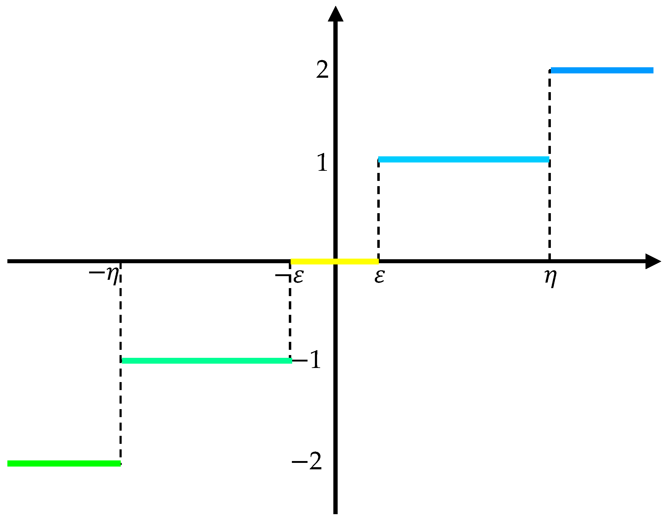
Figure 1. Module division principle.
Fractalfract 06 00345 g001
Figure 2. Algorithm flowchart: (a) SlEn; (b) PSO-SlEn; (c) FrSlEn; (d) PSO-FrSlEn.
Fractalfract 06 00345 g002aFractalfract 06 00345 g002b
Figure 3. The flowchart of the proposed feature extraction methods.
Fractalfract 06 00345 g003
Figure 4. The normalized 10 bearing signals: (a) N-100; (b) IR-108; (c) B-121; (d) OR-133; (e) IR-172; (f) B-188; (g) OR-200; (h) IR-212; (i) B-225; (j) OR-237.
Fractalfract 06 00345 g004aFractalfract 06 00345 g004b
Figure 5. Single feature distribution of PSO-FrSlEn: (a) α = 0.3 ; (b) α = 0.3 ; (c) α = 0.2 ; (d) α = 0.2 ; (e) α = 0.1 ; (f) α = 0.1 ; (g) α = 0 .
Fractalfract 06 00345 g005aFractalfract 06 00345 g005b
Figure 6. Classification results and distribution of PSO-FrSlEn: (a) α = 0.3 ; (b) α = 0.3 ; (c) α = 0.2 ; (d) α = 0.2 ; (e) α = 0.1 ; (f) α = 0.1 ; (g) α = 0 .
Fractalfract 06 00345 g006aFractalfract 06 00345 g006b
Figure 7. The classification accuracies under different fractional orders.
Fractalfract 06 00345 g007
Figure 8. Double feature distribution of the nine highest classification accuracies: (a) FrPE, α = 0.3 & 0 ; (b) FrWPE,   α = 0.3 & 0.3 ; (c) FrDE, α = 0.1 & 0.3 ; (d) FrFDE,   α = 0.3 & 0.1 ; (e) PSO-FrSlEn, α = 0.3 & 0.2 ; (f) PSO-FrSlEn, α = 0.2 & 0.2 ; (g) PSO-FrSlEn, α = 0.1 & 0.1 ; (h) PSO-FrSlEn, α = 0.1 & 0.2 ; (i) PSO-FrSlEn,   α = 0 & 0.1 .
Fractalfract 06 00345 g008aFractalfract 06 00345 g008b
Figure 9. The classification accuracies under different double feature combinations.
Fractalfract 06 00345 g009
Table 1. The classification accuracy of each entropy under different fractional orders.
FigureFrPE Accuracy (%)FrWPE Accuracy (%)FrDE Accuracy (%)FrFDE Accuracy (%)PSO-FrSlEn Accuracy (%)
−0.364.6746.6782.6777.3388
−0.278.6760.6781.3373.3384
−0.176.6766.6780.6779.3383.33
076.6769.3369.3379.3381.33
0.175.3369.338079.3386
0.275.3369.338280.6785.33
0.36672.7682.678083.33
Table 2. The highest accuracy of each entropy under different double feature combinations.
EntropyFractional Order CombinationsAccuracy (%)
FrPE 0.3 & 0 78.67
FrWPE 0.3 & 0.3 72.67
FrDE 0.1 & 0.3 96
FrFDE 0.3 & 0.1 89.33
PSO-FrSlEn 0.3 & 0.2 100
0.2 & 0.2 100
0.1 & 0.1 100
0.1 & 0.2 100
0 & 0.1 100
Publisher’s Note: MDPI stays neutral with regard to jurisdictional claims in published maps and institutional affiliations.