On the Modeling of COVID-19 Transmission Dynamics with Two Strains: Insight through Caputo Fractional Derivative

Abstract

The infection dynamics of COVID-19 is difficult to contain due to the mutation nature of the SARS-CoV-2 virus. This has been a public health concern globally with the impact of the pandemic on the world’s economy and mode of living. In the present work, we formulate and examine a fractional model of COVID-19 considering the two variants of concern on the disease transmission pathways, namely SARS-CoV-2 and D614G on our model formulation. The existence and uniqueness of our model solutions were analyzed using the fixed point theory. Mathematical analyses were presented, and the model’s basic reproduction numbers ${\mathcal{R}}_{01}$ and ${\mathcal{R}}_{02}$ were determined. The model has three equilibria: the disease-free equilibrium, that endemic for strain 1, and that endemic for strain 2. The locally asymptotic stability of the equilibria was established based on the ${\mathcal{R}}_{01}$ and ${\mathcal{R}}_{02}$ values. Caputo fractional operator was used to simulate the model to study the dynamics of the model solution. Results from numerical simulations envisaged that an increase in the transmission parameters of strain 1 leads to an increase in the number of infected individuals. On the other hand, an increase in the strain 2 transmission rate gives rise to more infection. Furthermore, it was established that there is an increased number of infections with a negative impact of strain 1 on strain 2 dynamics and vice versa.

1. Introduction

Coronavirus disease (COVID-19) is an infectious illness caused by SARS-CoV-2. The first case was announced in Wuhan, China on 31 December 2019 [1]. COVID-19 transmission can occur from human to human through splashes from the nose or mouth that come out through coughing, sneezing, talking, singing, or breathing heavily. In addition, contagion can also occur when a healthy person touches the surface of droplet-contaminated objects around an infected person [1]. The COVID-19 disease has a negative effect on people’s lives, including psychological, economic, and social effects. The COVID-19 pandemic also increases the risk of suicide due to lockdown, social distancing, and financial crisis. Measures that can minimize the spread of COVID-19 include educating the public about the efforts to prevent the spread of COVID-19 [2]. Other preventive measures include the use of masks when around others, washing hands as often as possible, keeping at least 6 feet away from others, staying home and isolating yourself from others when sick, avoiding crowds, avoiding poorly ventilated rooms, covering your mouth with tissues when coughing and sneezing, and routinely cleaning surfaces that are frequently touched [3]. According to the World Health Organisation (WHO), there were 85,091,012 cases of COVID-19 with 1,861,005 deaths worldwide as of 6 January 2021 [4].

Before the COVID-19 outbreak, there were six different coronaviruses species that could infect humans, namely HCoV-229E, HCoV-NL63, HCoV-OC43, HCoV-HKU1, SARS-CoV, and MERS-CoV [5]. Common symptoms of COVID-19 infection incorporate acute respiratory disorders such as fever, cough, and shortness of breath [6]. SARS-CoV-2 is a virus that can mutate and produce new strains. One mutation of SARS-CoV-2 is D614G. The D614G strains is an amino acid mutation in position 614 that results in a change from D (aspartic acid) to G (glycine) [7]. The D614G strains is the most dominant variant in the world because it spreads faster than other types and tends to be more contagious [8]. The SARS-CoV-2 variants have been classified by CDC and the U.S government SARS-CoV-2 Interagency Group (SIG) into four categories [9]: (i) Variant being monitored, which consists of Alpha, Beta, Gamma, Delta, Epsilon, Eta, Iota, Kappa, Mu, and Zeta (P.2), (ii) Variant of interest, (iii) Variant of concern: Omicron and (iv) Variant of high consequence. The Omicron variant (B.1.1.529) was declared a variant of concern by the WHO on 26 November 2021 [10]. Since the detection of the Omicron variant in South Africa via genome sequencing [11], it has also spread rapidly across the globe with an increase in the new number of daily COVID-19 cases, which is linked to the Omicron variant [4]. In particular, the Omicron variant has about 60 mutations from the original wild-type variant that emanated originally from Wuhan, China, in 2020, with more than 30 in the spike protein [12]. These spike mutations of Omicron have prominent significant concerns about current vaccines’ potential effectiveness and the level of immunity conferred from previous infections of COVID-19. In addition, it also has increased transmissibility, hospitalization rate, mortality, disease severity, and decreased vaccine-induced protection from severe disease as well as neutralization by antibodies generated during previous infection or after vaccination [9].

Since COVID-19 was declared by the WHO as a global pandemic, a number of mathematical models have been elaborated to conceive the spread of COVID-19. Some of the research work done in the field of mathematical modeling related to the COVID-19 problem applied both integer [13,14,15,16,17,18,19,20] and fractional order in their modeling frameworks [21,22,23,24,25,26,27]. Fractional calculus, which uses fractional derivatives (FD), is a new rapidly growing area in mathematical science that picks up a memory effect and hereditary characteristics of various physical and natural phenomena occurring in engineering, technology, physical and natural sciences [28,29,30]. The most widely used FD includes the Caputo, Caputo–Fabrizio (CF) and Atangana–Baleanu–Caputo fractional-order operators. Other researchers have also analyzed COVID-19 by exploring possible control measures to mitigate the spread of the virus through the application of fractional derivative theory. The authors in [24] proposed a fractional-order model which considers the effect of the pathogens in the environment and vaccination on the transmission dynamics of COVID-19 in Indonesia. Their finding suggests that a decrease in the pathogen level will reduce the number of infected individuals in the human population, which helps reduce the spread of the disease.

Recent work on COVID-19 modeling which incorporates two strains includes models with vaccination [31], optimal control [32], vaccination scale-up [33], with pre-symptomatic individuals [34] and non-pharmaceutical interventions [35] in the form integer model. It is essential to explore the COVID-19 transmission caused by two different types of variants using a mathematical framework. Limited evidence indicates that those who recover from the disease can be reinfected again when there is a new strain but at a rate less severe than the previous infection. Therefore, we investigate the potential impact of two variants on the COVID-19 transmission pathway by considering a case scenario where it was caused by two different strains of the SARS-CoV-2 variants. We are now motivated in the present study to modify the mathematical model of the spread of COVID-19 that was developed by Rezapour et al. [21] by including a transmission path with two strains. The model initially did not consider strains of the COVID virus in the modeling approach. Therefore, to further refine the work in [21], we considered two strains of the virus, namely SARS-CoV-2 and D614G, in our modeling approach by applying the Caputo operator. The fractional model leads to more interesting and unique findings than the integer model due to providing a better understanding of disease dynamics. For example, the authors in [24] indicated that the Caputo model gives a preferable approximation to the reported infected cases.

Furthermore, the model modifications made include dividing the population of exposed individuals into two, based on the strain of the virus, that is, the exposed population to strain 1 and the exposed population to strain 2. In addition, the population of infected individuals is divided into those infected with strain 1 and those infected with strain 2. The CF basic mathematical preliminaries is discussed in the next section.

2. Basic Caputo Fractional-Order Preliminaries

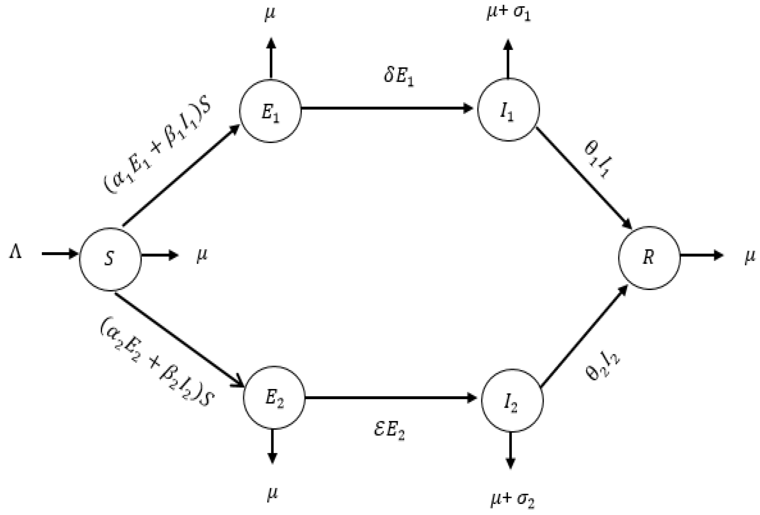
Here, we provide the basic definitions for fractional calculus that will be employed to consider the COVID-19 model with two strains.

Definition 1.

According to [36], let $\chi \in {\mathcal{C}}^n$ be a function; then, the Caputo derivative with a fractional order $\sigma \in (n-1,n)$ for $n\in \mathbb{N}$ is defined to be

$$\begin{array}{c}{\displaystyle {}^{\mathcal{C}}{\mathcal{D}}_t^{\sigma }\left(\chi \left(t\right)\right)={\displaystyle \frac{1}{\Gamma (n-\sigma )}}{\int }_0^t\frac{d^n}{d{t}^n}\chi \left(\phi \right){(t-\phi )}^{n-\sigma -1}d\phi .}\hfill \end{array}$$

Thus, it is obviously that ${}^{\mathcal{C}}{\mathcal{D}}_t^{\sigma }\left(\chi \left(t\right)\right)\to \chi {\left(t\right)}^{\prime }$ if $\sigma \to 1.$

Definition 2.

According to Definition 1, the integral operator for the function $\chi :\mathbb{R}\to \mathbb{B}$ with order $\sigma \ge 0$ is given by

$$\begin{array}{c}{\displaystyle {}^{\mathcal{C}}{\mathcal{I}}_t^{\sigma }\left(\chi \left(t\right)\right)={\displaystyle \frac{1}{\Gamma \left(\sigma \right)}}{\int }_0^t\chi \left(\phi \right){(t-\phi )}^{(\sigma -1)}d\phi .}\hfill \end{array}$$

for $0<\sigma <1,t>0.$

Lastly, we give the definition which denotes the equilibrium for Caputo fractional model. Hence, it is established as follows

Definition 3.

According to [37], if ${\chi }^{*}$ is the equilibrium point, then

$$\begin{array}{c}{\displaystyle {}^{\mathcal{C}}{\mathcal{D}}_t^{\sigma }\left(\chi \left(t\right)\right)=f(t,\chi \left(t\right))}\hfill \end{array}$$

for $\sigma \in (0,1)$ if and only if $f(t,{\chi }^{*})=0$

The remaining of the paper is arranged as follows. Section 3 explains details of the model formulation followed by model analyses in Section 4. Meanwhile, Section 5 presents the numerical simulations and Section 6 summarizes the main finding of the paper.

3. The Model

In this section, we describe a mathematical model of the spread of COVID-19 with two strains. The model consists of six subpopulations, namely, the susceptible class $\left(S\right)$, the class of individuals exposed to strain 1 ($E_1$), the class of individuals exposed to strains 2 ($E_2$), infected with strains 1 ($I_1$), infected with strain 2 ($I_2$), and recovered class from either strain 1 or 2 $\left(R\right).$ Thus, the total population at any time t is given by $N\left(t\right)=S\left(t\right)+E_1\left(t\right)+E_2\left(t\right)+I_1\left(t\right)+I_2\left(t\right)+R\left(t\right).$ The explicit notation and description of each variable and parameter used in this mathematical model are given in Table 1.

Table 1. Parameters of the COVID-19 model with two strains.

Symbol	Description	Units
$\Lambda$	Recruitment rate	$\frac{Individual}{time}$
$\mu$	Natural death rate	$\frac{1}{time}$
${\alpha }_1$	Transmission rate by $E_1$	$\frac{1}{time}$
${\alpha }_2$	Transmission rate by $E_2$	$\frac{1}{time}$
${\beta }_1$	Transmission rate by $I_1$	$\frac{1}{time}$
${\beta }_2$	Transmission rate by $I_2$	$\frac{1}{time}$
$\delta$	Progression rate from $E_1$ to $I_1$	$\frac{1}{time}$
$\mathcal{E}$	Progression rate from $E_2$ to $I_2$	$\frac{1}{time}$
${\sigma }_1$	Death rate due to strain 1	$\frac{1}{time}$
${\sigma }_2$	Death rate due to strain 2	$\frac{1}{time}$
${\theta }_1$	Recovery rate of infected with strain 1	$\frac{1}{time}$
${\theta }_2$	Recovery rate of infected with strain 2	$\frac{1}{time}$

Our model is built based on the following assumptions in terms of COVID-19 with two strains; (1) both the exposed and infected with strains 1 and 2 populations can transmit the disease; (2) the transmission rate of the infected individual with strain 2 is greater than that of the infected individuals with strain 1; (3) the transmission rate of individuals exposed to strain 2 is greater than that of individuals exposed to strain 1; (4) only the infected individuals die from the disease; (5) the recovered individuals cannot be reinfected.

Based on the notation and assumptions, a transmission diagram of the mathematical model of the spread of COVID-19 with two strains can be constructed as shown in Figure 1.

Figure 1. Transmission diagram of the COVID-19 model with two strains.

Combining the transmission diagram shown in Figure 1 and the model assumptions, we have the following ordinary differential equation (ODE) governing our mathematical model for the spread of COVID-19 with two strains, which we shall explain in detail. Equation (1) represents the rate of change of the susceptible individual population to the unit of time. Susceptible populations can increase due to the recruitment rate and decrease due to interactions between susceptible and exposed individuals to strain 1 and individuals infected with strain 1. In addition, susceptible populations can also decrease due to interactions between the susceptible and exposed individuals to strain 2 and individuals infected with strain 2. The population can also be reduced due to the natural death rate.

$$\frac{dS}{dt}=\Lambda -\left({\alpha }_1{E}_1+{\beta }_1{I}_1\right)S-\left({{\alpha }_{2}E}_2+{\beta }_2{I}_2\right)S-\mu S.$$

(1)

Equation (2) represents the rate of change of the population of individuals exposed to strain 1. This population increases because of the interaction between susceptible individuals and individuals exposed to strain 1 and infected with strain 1. This population can decrease due to the rate of development from individuals exposed to strain 1 to individuals infected with strain 1. The population can also decrease due to the natural death rate.

$$\frac{d{E}_1}{dt}=\left({\alpha }_1{E}_1+{\beta }_1{I}_1\right)S-p{E}_1$$

(2)

where $p=(\mu +\delta ).$

Equation (3) represents the rate of change of the population of individuals infected with strain 1. This population increases because of the rate of transition of individuals exposed to strain 1 to individuals infected with strain 1. The population can decrease due to the natural death rate and death rate due to strain 1. In addition, the population can also decrease due to the recovery rate of individuals infected with strain 1.

$$\frac{d{I}_1}{dt}=\delta E_1-q{I}_1$$

(3)

for $q=(\mu +{\sigma }_1+{\theta }_1).$

Equation (4) represents the rate of change of the population of individuals exposed to strain 2. This population increases because of the interaction between susceptible individuals and individuals exposed to strain 2 and individuals infected with strain 2. This population can decrease due to the rate of development from individuals exposed to strain 2 to individuals infected with strain 2. It can also decrease due to the natural death rate.

$$\frac{d{E}_2}{dt}=\left({{\alpha }_{2}E}_2+{\beta }_2{I}_2\right)S-r{E}_2$$

(4)

in which $r=(\mu +\mathcal{E}).$

Equation (5) represents the rate of change of the population of individuals infected with strain 2 with respect to time. This population increases because of the rate of development of individuals exposed to strain 2 to individuals infected with strain 2. The population can decrease due to the natural death rate and death rate due to strain 2. In addition, the population can also decrease due to the recovery rate of individuals infected with strain 2.

$$\frac{d{I}_2}{dt}=\mathcal{E}{E}_2-w{I}_2$$

(5)

for $w=(\mu +{\sigma }_2+{\theta }_2).$

Equation (6) represents the rate of change of population of individuals recovered from both strains. This population increases because of the recovery rate of individuals infected with strain 1 and the rate of recovery of individuals infected with strain 2. The population can decrease due to the natural death rate.

$$\frac{d\mathrm{R}}{dt}={\theta }_1{I}_1+{\theta }_2{I}_2-\mu R.$$

(6)

Therefore, combining Equations (1)–(6), we have the general system of ODE describing COVID-19 transmission pathways with two trains:

$$\left\{\begin{array}{l}{\displaystyle \frac{dS}{dt}=\Lambda -\left({\alpha }_1{E}_1+{\beta }_1{I}_1\right)S-\left({{\alpha }_{2}E}_2+{\beta }_2{I}_2\right)S-\mu S,}\\ \\ {\displaystyle \frac{d{E}_1}{dt}=\left({\alpha }_1{E}_1+{\beta }_1{I}_1\right)S-p{E}_1,}\\ \\ {\displaystyle \frac{d{I}_1}{dt}=\delta E_1-q{I}_1,}\\ \\ {\displaystyle \frac{d{E}_2}{dt}=\left({{\alpha }_{2}E}_2+{\beta }_2{I}_2\right)S-r{E}_2,}\hfill \\ \\ {\displaystyle \frac{d{I}_2}{dt}=\mathcal{E}{E}_2-w{I}_2,}\hfill \\ \\ {\displaystyle \frac{dR}{dt}={\theta }_1{I}_1+{\theta }_2{I}_2-\mu R,}\hfill \end{array}\right.$$

(7)

subject to the initial conditions

$$\begin{array}{c}S\left(0\right)>0,E_1\left(0\right)\ge 0,I_1\left(0\right)\ge 0,E_2\left(0\right)\ge 0,I_2\left(0\right)\ge 0,R\left(0\right)\ge 0.\hfill \end{array}$$

We transform the model Equation (7) into a fractional differential model, which yields

$$\left\{\begin{array}{c}{\displaystyle {}^C{\mathcal{D}}_t^{\sigma }S\left(t\right)={\displaystyle \frac{1}{\Gamma (1-\sigma )}}{\int }_0^t{(t-\phi )}^{-\sigma }{S}^{\prime }\left(\phi \right)d\phi ,}\hfill \\ \\ {\displaystyle {}^C{\mathcal{D}}_t^{\sigma }{E}_1\left(t\right)={\displaystyle \frac{1}{\Gamma (1-\sigma )}}{\int }_0^t{(t-\phi )}^{-\sigma }{E}_1^{\prime }\left(\phi \right)d\phi ,}\hfill \\ \\ {\displaystyle {}^C{\mathcal{D}}_t^{\sigma }{I}_1\left(t\right)={\displaystyle \frac{1}{\Gamma (1-\sigma )}}{\int }_0^t{(t-\phi )}^{-\sigma }{I}_1^{\prime }\left(\phi \right)d\phi ,}\hfill \\ \\ {\displaystyle {}^C{\mathcal{D}}_t^{\sigma }{E}_2\left(t\right)={\displaystyle \frac{1}{\Gamma (1-\sigma )}}{\int }_0^t{(t-\phi )}^{-\sigma }{E}_2^{\prime }\left(\phi \right)d\phi ,}\hfill \\ \\ {\displaystyle {}^C{\mathcal{D}}_t^{\sigma }{I}_2\left(t\right)={\displaystyle \frac{1}{\Gamma (1-\sigma )}}{\int }_0^t{(t-\phi )}^{-\sigma }{I}_2^{\prime }\left(\phi \right)d\phi ,}\hfill \\ {\displaystyle {}^C{\mathcal{D}}_t^{\sigma }R\left(t\right)={\displaystyle \frac{1}{\Gamma (1-\sigma )}}{\int }_0^t{(t-\phi )}^{-\sigma }{R}^{\prime }\left(\phi \right)d\phi .}\hfill \end{array}\right.$$

(8)

Using the Caputo operator, we covert system (7) to a fractional ODE system:

$$\left\{\begin{array}{c}{\displaystyle {}_0^C{\mathcal{D}}_t^{\sigma }S\left(t\right)=\Lambda -\left({\alpha }_1{E}_1\left(t\right)+{\beta }_1{I}_1\left(t\right)\right)S\left(t\right)-\left({{\alpha }_{2}E}_2+{\beta }_2{I}_2\left(t\right)\right)S\left(t\right)-\mu S\left(t\right),}\hfill \\ {\displaystyle {}_0^C{\mathcal{D}}_t^{\sigma }{E}_1\left(t\right)=\left({\alpha }_1{E}_1\left(t\right)+{\beta }_1{I}_1\left(t\right)\right)S\left(t\right)-p{E}_1\left(t\right),}\hfill \\ {\displaystyle {}_0^C{\mathcal{D}}_t^{\sigma }{I}_1\left(t\right)=\delta E_1\left(t\right)-q{I}_1\left(t\right),}\hfill \\ {\displaystyle {}_0^C{\mathcal{D}}_t^{\sigma }{E}_2\left(t\right)=\left({\alpha }_2{E}_2\left(t\right)+{\beta }_2{I}_2\left(t\right)\right)S\left(t\right)-r{E}_2\left(t\right),}\hfill \\ {\displaystyle {}_0^C{\mathcal{D}}_t^{\sigma }{I}_2\left(t\right)=\mathcal{E}{E}_2\left(t\right)-w{I}_2\left(t\right),}\hfill \\ {\displaystyle {}_0^C{\mathcal{D}}_t^{\sigma }R\left(t\right)={\theta }_1{I}_1\left(t\right)+{\theta }_2{I}_2\left(t\right)-\mu R\left(t\right),}\hfill \end{array}\right.$$

(9)

subjective to initial conditions

$$\begin{array}{c}{}_0^C{\mathcal{D}}_t^{\sigma }S\left(0\right)>0,{}_0^C{\mathcal{D}}_t^{\sigma }{E}_1\left(0\right)\ge 0,{}_0^C{\mathcal{D}}_t^{\sigma }{I}_1\left(0\right)\ge 0,{}_0^C{\mathcal{D}}_t^{\sigma }{E}_2\left(0\right)\ge 0,{}_0^C{\mathcal{D}}_t^{\sigma }{I}_2\left(0\right)\ge 0,{}_0^C{\mathcal{D}}_t^{\sigma }R\left(0\right)\ge 0.\hfill \end{array}$$

The parameters of the model and state variables are assumed to be positive over the modeling time horizon.

4. Mathematical Analyses

In this section, we establish some basic properties of our model (9).

4.1. Basic Properties of the Fractional Model

We verify that the fractional model (9) is positive, bounded, and biologically meaningful over the modeling time for $t\ge 0.$

Proof. 

The total dynamic of the fractional model (9) is given by the following equation

$$\begin{array}{ccc}{\displaystyle {}_0^C{\mathcal{D}}_t^{\tau }N\left(t\right)}\hfill & =\hfill & {\displaystyle {}_0^C{\mathcal{D}}_t^{\tau }S\left(t\right){+}_0^C{\mathcal{D}}_t^{\tau }{E}_1\left(t\right){+}_0^C{\mathcal{D}}_t^{\tau }{I}_1\left(t\right){+}_0^C{\mathcal{D}}_t^{\tau }{E}_2\left(t\right){+}_0^C{\mathcal{D}}_t^{\tau }{I}_2\left(t\right){+}_0^C{\mathcal{D}}_t^{\tau }R\left(t\right),}\hfill \\ \hfill & =\hfill & \Lambda -\mu N-(q+w),\hfill \\ \hfill & \le \hfill & \Lambda -\mu N.\hfill \end{array}$$

(10)

The solutions of (10) yield

$${\displaystyle N\left(t\right)\le N\left(0\right){\mathfrak{E}}_{\sigma ,1}(-\mu t^{\sigma })+\Lambda t^{\sigma }{\mathfrak{E}}_{\sigma ,\sigma +1}(-\mu t^{\sigma }),}$$

where ${\mathfrak{E}}_{\sigma ,\sigma +1}$ is the Mittag–Leffler function defined by ${\mathfrak{E}}_{\sigma ,\sigma +1}\left(t\right)={\Sigma }_{k=0}^{\infty }{\displaystyle \frac{t^k}{\Gamma (\sigma k+(\sigma +1\left)\right)}}.$

We obtain ${\displaystyle N\left(t\right)\le {\displaystyle \frac{\Lambda }{\mu }}}$ when $t\to \infty .$

The biological feasible region $\overline{\Gamma }$ of the COVID-19 model with two strains is expressed by

$${\displaystyle \overline{\overline{\Gamma }}=\left\{\left(S\left(t\right),E_1\left(t\right),I_1\left(t\right),E_2\left(t\right),I_2\left(t\right),R\left(t\right)\right)\in {\mathbb{R}}_{+}^6\le {\displaystyle \frac{\Lambda }{\mu }}\right\}.}$$

Hence, the fractional model (9) which incorporates two strains is biologically feasible and bounded for all time $t\ge 0.$ □

4.2. Existence and Uniqueness of Solutions

Now, we examine and prove the existence and uniqueness of the solutions of the model (9) with the initial condition using the fixed point theory.

Let $\mathcal{G}\left(\mathcal{Q}\right)$ be the Banach space of the real valued continuous function over $\mathcal{Q}=[0,c]$ with the norm given by

$$\left|\right|S\left|\right|=\underset{t\in \mathcal{Q}}{sup}\left|S\left(t\right)\right|,\left|\right|E_1\left|\right|=\underset{t\in \mathcal{Q}}{sup}|E_1\left(t\right)|,||I_1\left|\right|=\underset{t\in \mathcal{Q}}{sup}|I_1\left(t\right)|,||E_2\left|\right|=\underset{t\in \mathcal{Q}}{sup}\left|E_2\left(t\right)\right|,$$

$\left|\right|I_2\left|\right|={sup}_{t\in \mathcal{Q}}\left|I_2\left(t\right)\right|$ and $\left|\right|R\left|\right|={sup}_{t\in \mathcal{Q}}\left|R\left(t\right)\right|.$

Further, we also have the norm

$$\left|\right|S\left(t\right),E_1\left(t\right),I_1\left(t\right),E_2\left(t\right),I_2\left(t\right),R\left(t\right)\left|\right|=\left|\right|S\left(t\right)\left|\right|+\left|\right|E_1\left(t\right)\left|\right|+\left|\right|I_1\left(t\right)\left|\right|+\left|\right|E_2\left(t\right)\left|\right|+$$

$$\left|\right|I_2\left(t\right)\left|\right|+\left|\right|R\left(t\right)\left|\right|.$$

Proof. 

We transform the model (9) using the Caputo integral

$$\begin{array}{cc}\hfill {\displaystyle S\left(t\right)=}& {\displaystyle S\left(0\right){+}^C{\mathcal{D}}_t^{\sigma }\left\{\Lambda -\left({\alpha }_1{E}_1+{\beta }_1{I}_1\right)S-\left({{\alpha }_{2}E}_2+{\beta }_2{I}_2\right)S-\mu S\right\},}\hfill \\ \hfill {\displaystyle E_1\left(t\right)=}& {\displaystyle E_1\left(0\right){+}^C{\mathcal{D}}_t^{\sigma }\left\{\left({\alpha }_1{E}_1+{\beta }_1{I}_1\right)S-p{E}_1\right\},}\hfill \\ \hfill {\displaystyle I_1\left(t\right)=}& {\displaystyle I_1\left(0\right){+}^C{\mathcal{D}}_t^{\sigma }\left\{\delta E_1-q{I}_1\right\},}\hfill \\ \hfill {\displaystyle E_2\left(t\right)=}& {\displaystyle E_2\left(0\right){+}^C{\mathcal{D}}_t^{\sigma }\left\{\left({\alpha }_2{E}_2+{\beta }_2{I}_2\right)S-r{E}_2\right\},}\hfill \\ \hfill {\displaystyle I_2\left(t\right)=}& {\displaystyle I_2\left(0\right){+}^C{\mathcal{D}}_t^{\sigma }\left\{\mathcal{E}{E}_2-w{I}_2\right\}}\hfill \\ \hfill {\displaystyle R\left(t\right)=}& {\displaystyle R\left(0\right){+}^C{\mathcal{D}}_t^{\sigma }\left\{{\theta }_1{I}_1+{\theta }_2{I}_2-\mu R\right\}}\hfill \end{array}$$

Utilizing Definition (2), we obtain

$$\left\{\begin{array}{cc}\hfill {\displaystyle S\left(t\right)=}& {\displaystyle S\left(0\right)+{\displaystyle \frac{1}{\Gamma \left(\sigma \right)}}{\int }_0^t{(t-\phi )}^{\sigma -1}{F}_1(\phi ,S\left(\phi \right))d\phi ,}\hfill \\ \hfill {\displaystyle E_1\left(t\right)=}& {\displaystyle E_1\left(0\right)+{\displaystyle \frac{1}{\Gamma \left(\sigma \right)}}{\int }_0^t{(t-\phi )}^{\sigma -1}{F}_2(\phi ,E_1\left(\phi \right))d\phi ,}\hfill \\ \hfill {\displaystyle I_1\left(t\right)=}& {\displaystyle I_1\left(0\right)+{\displaystyle \frac{1}{\Gamma \left(\sigma \right)}}{\int }_0^t{(t-\phi )}^{\sigma -1}{F}_3(\phi ,I_1\left(\phi \right))d\phi ,}\hfill \\ \hfill {\displaystyle E_2\left(t\right)=}& {\displaystyle E_2\left(0\right)+{\displaystyle \frac{1}{\Gamma \left(\sigma \right)}}{\int }_0^t{(t-\phi )}^{\sigma -1}{F}_4(\phi ,E_2\left(\phi \right))d\phi ,}\hfill \\ \hfill {\displaystyle I_2\left(t\right)=}& {\displaystyle I_2\left(0\right)+{\displaystyle \frac{1}{\Gamma \left(\sigma \right)}}{\int }_0^t{(t-\phi )}^{\sigma -1}{F}_5(\phi ,I_2\left(\phi \right))d\phi ,}\hfill \\ \hfill {\displaystyle R\left(t\right)=}& {\displaystyle R\left(0\right)+{\displaystyle \frac{1}{\Gamma \left(\sigma \right)}}{\int }_0^t{(t-\phi )}^{\sigma -1}{F}_6(\phi ,R\left(\phi \right))d\phi ,}\hfill \end{array}\right.$$

(11)

with the following kernels:

$$\left\{\begin{array}{cc}{\displaystyle F_1(t,S\left(t\right))=}\hfill & {\displaystyle \Lambda -\left({\alpha }_1{E}_1+{\beta }_1{I}_1\right)S-\left({{\alpha }_{2}E}_2+{\beta }_2{I}_2\right)S-\mu S,}\hfill \\ {\displaystyle F_2(t,E_1\left(t\right))=}\hfill & {\displaystyle \left({\alpha }_1{E}_1+{\beta }_1{I}_1\right)S-p{E}_1,}\hfill \\ {\displaystyle F_3(t,I_1\left(t\right))=}\hfill & {\displaystyle \delta E_1-q{I}_1,}\hfill \\ {\displaystyle F_4(t,E_2\left(t\right))=}\hfill & {\displaystyle \left({\alpha }_2{E}_2+{\beta }_2{I}_2\right)S-r{E}_2,}\hfill \\ {\displaystyle F_5(t,I_2\left(t\right))=}\hfill & {\displaystyle \mathcal{E}{E}_2-w{I}_2}\hfill \\ {\displaystyle F_5(t,R\left(t\right))=}\hfill & {\displaystyle {\theta }_1{I}_1+{\theta }_2{I}_2-\mu R.}\hfill \end{array}\right.$$

(12)

The expression $F_j$ in Equation (12) for $j=1,\cdots ,6$ fulfills the Lipschitz for the model variables $(S\left(t\right),E_1\left(t\right),I_1\left(t\right),E_2\left(t\right),I_2\left(t\right),R\left(t\right))$ that hold an upper bound. Firstly, we provide the proof for the S variable. Let S and $\tilde{S}$ be two different functions. We examine the proof for $S\left(t\right).$

$${\displaystyle \left|\right|F_1(t,S\left(t\right))-F_1(t,\tilde{S}\left(t\right))\left|\right|=\left|\right|\left(\left({\alpha }_1{E}_1+{\beta }_1{I}_1\right)-\left({{\alpha }_{2}E}_2+{\beta }_2{I}_2\right)-\mu \right)(S\left(t\right)-\tilde{S}\left(t\right))\left|\right|.}$$

Setting ${\zeta }_1=\left(\right||\left({\alpha }_1{E}_1+{\beta }_1{I}_1\right)+\left({{\alpha }_{2}E}_2+{\beta }_2{I}_2\right)+\mu \left|\right|)$, we get

$$\left|\right|F_1(t,S\left(t\right))-F_1(t,\overline{S}\left(t\right))\left|\right|\le {\zeta }_1\left|\right|S\left(t\right)-\overline{S}\left(t\right)\left|\right|.$$

Likewise, for the continuing of state variables, we carry that

$$\begin{array}{cc}{\displaystyle \left|\right|F_2(t,E_1\left(t\right))-F_2(t,\widetilde{E_1}\left(t\right))\left|\right|\le }\hfill & {\displaystyle {\zeta }_2\left|\right|E_1\left(t\right)-\widetilde{E_1}\left(t\right)\left|\right|,}\hfill \\ {\displaystyle \left|\right|F_3(t,I_1\left(t\right))-F_3(t,\widetilde{I_1}\left(t\right))\left|\right|\le }\hfill & {\displaystyle {\zeta }_3\left|\right|I_1\left(t\right)-\widetilde{I_1}\left(t\right)\left|\right|,}\hfill \\ {\displaystyle \left|\right|F_4(t,E_2\left(t\right))-F_4(t,\widetilde{E_2}\left(t\right))\left|\right|\le }\hfill & {\displaystyle {\zeta }_4\left|\right|E_2\left(t\right)-\widetilde{E_2}\left(t\right)\left|\right|,}\hfill \\ {\displaystyle \left|\right|F_5(t,I_2\left(t\right))-F_5(t,\widetilde{I_2}\left(t\right))\left|\right|\le }\hfill & {\displaystyle {\zeta }_5\left|\right|I_2\left(t\right)-\widetilde{I_2}\left(t\right)\left|\right|,}\hfill \\ {\displaystyle \left|\right|F_6(t,R\left(t\right))-F_6(t,\tilde{R}\left(t\right))\left|\right|\le }\hfill & {\displaystyle {\zeta }_6\left|\right|R\left(t\right)-\tilde{R}\left(t\right)\left|\right|,}\hfill \end{array}$$

where ${\zeta }_1,{\zeta }_2,{\zeta }_3,{\zeta }_4,{\zeta }_5$ and ${\zeta }_6$ assert the Lipschitz constants for each kernel $F_j$ for $j=1,\cdots ,6$ respectively. Hence, the Lipschitz condition is fulfilled. To finish the uniqueness proof by employing the Banach theory, we also represent that system (11) is recursive in nature. Therefore

$$\left\{\begin{array}{cc}\hfill {\displaystyle S_n\left(t\right)=}& {\displaystyle S\left(0\right)+{\displaystyle \frac{1}{\Gamma \left(\sigma \right)}}{\int }_0^t{(t-\phi )}^{\sigma -1}{F}_1(\phi ,S_{n-1}\left(\phi \right))d\phi ,}\hfill \\ \\ \hfill {\displaystyle {E_1}_n\left(t\right)=}& {\displaystyle E_{18}\left(0\right)+{\displaystyle \frac{1}{\Gamma \left(\sigma \right)}}{\int }_0^t{(t-\phi )}^{\sigma -1}{F}_2(\phi ,E_{1(n-1)}\left(\phi \right))d\phi ,}\hfill \\ \\ \hfill {\displaystyle {I_1}_n\left(t\right)=}& {\displaystyle I_1\left(0\right)+{\displaystyle \frac{1}{\Gamma \left(\sigma \right)}}{\int }_0^t{(t-\phi )}^{\sigma -1}{F}_3(\phi ,I_{1(n-1)}\left(\phi \right))d\phi ,}\hfill \\ \\ \hfill {\displaystyle {E_2}_n\left(t\right)=}& {\displaystyle E_2\left(0\right)+{\displaystyle \frac{1}{\Gamma \left(\sigma \right)}}{\int }_0^t{(t-\phi )}^{\sigma -1}{F}_4(\phi ,E_{2(n-1)}\left(\phi \right))d\phi ,}\hfill \\ \\ \hfill {\displaystyle {I_2}_n\left(t\right)=}& {\displaystyle I_2\left(0\right)+{\displaystyle \frac{1}{\Gamma \left(\sigma \right)}}{\int }_0^t{(t-\phi )}^{\sigma -1}{F}_5(\phi ,I_{2(n-1)}\left(\phi \right))d\phi ,}\hfill \\ \\ \hfill {\displaystyle R_n\left(t\right)=}& {\displaystyle R\left(0\right)+{\displaystyle \frac{1}{\Gamma \left(\sigma \right)}}{\int }_0^t{(t-\phi )}^{\sigma -1}{F}_6(\phi ,R_{n-1}\left(\phi \right))d\phi .}\hfill \end{array}\right.$$

(13)

After some algebraic calculations of the difference between the successive expression together with the initial conditions, we obtain

$$\left\{\begin{array}{cc}\hfill {\displaystyle {\Phi }_{S,n}\left(t\right)=}& {\displaystyle S_n\left(t\right)-S_{n-1}\left(t\right)={\displaystyle \frac{1}{\Gamma \left(\sigma \right)}}{\int }_0^t{(t-\phi )}^{\sigma -1}\left(F_1(\phi ,S_{n-1}\left(\phi \right))-F_1(\phi ,S_{n-2}\left(\phi \right))\right)d\phi ,}\hfill \\ \\ \hfill {\displaystyle {\Phi }_{E_1,n}\left(t\right)=}& {\displaystyle {E_1}_n\left(t\right)-{E_1}_{n-1}\left(t\right)={\displaystyle \frac{1}{\Gamma \left(\sigma \right)}}{\int }_0^t{(t-\phi )}^{\sigma -1}\left(F_2(\phi ,V_{n-1}\left(\phi \right))-F_2(\phi ,V_{n-2}\left(\phi \right))\right)d\phi ,}\hfill \\ \\ \hfill {\displaystyle {\Phi }_{I_1,n}\left(t\right)=}& {\displaystyle {I_1}_n\left(t\right)-{I_1}_{n-1}\left(t\right)={\displaystyle \frac{1}{\Gamma \left(\sigma \right)}}{\int }_0^t{(t-\phi )}^{\sigma -1}\left(F_3(\phi ,E_{n-1}\left(\phi \right))-F_3(\phi ,E_{n-2}\left(\phi \right))\right)d\phi ,}\hfill \\ \\ \hfill {\displaystyle {\Phi }_{E_2,n}\left(t\right)=}& {\displaystyle {E_2}_n\left(t\right)-{E_2}_{n-1}\left(t\right)={\displaystyle \frac{1}{\Gamma \left(\sigma \right)}}{\int }_0^t{(t-\phi )}^{\sigma -1}\left(F_4(\phi ,I_{n-1}\left(\phi \right))-F_4(\phi ,{E_2}_{n-2}\left(\phi \right))\right)d\phi ,}\hfill \\ \\ \hfill {\displaystyle {\Phi }_{I_2,n}\left(t\right)=}& {\displaystyle {I_2}_n\left(t\right)-{I_2}_{n-1}\left(t\right)={\displaystyle \frac{1}{\Gamma \left(\sigma \right)}}{\int }_0^t{(t-\phi )}^{\sigma -1}\left(F_5(\phi ,{I_2}_{n-1}\left(\phi \right))-F_5(\phi ,{I_2}_{n-2}\left(\phi \right))\right)d\phi ,}\hfill \\ \\ \hfill {\displaystyle {\Phi }_{R,n}\left(t\right)=}& {\displaystyle R_n\left(t\right)-R_{n-1}\left(t\right)={\displaystyle \frac{1}{\Gamma \left(\sigma \right)}}{\int }_0^t{(t-\phi )}^{\sigma -1}\left(F_6(\phi ,R_{n-1}\left(\phi \right))-F_6(\phi ,R_{n-2}\left(\phi \right))\right)d\phi ,}\hfill \end{array}\right.$$

(14)

where in (14)

$$\begin{array}{cc}{\displaystyle S_n\left(t\right)=}\hfill & {\displaystyle \sum _{j=0}^n{\Phi }_{S,j}\left(t\right),{E_1}_n\left(t\right)=\sum _{j=0}^n{\Phi }_{E_1,j}\left(t\right),{I_1}_n\left(t\right)=\sum _{j=0}^n{\Phi }_{I_1,j}\left(t\right)}\hfill \\ {\displaystyle {E_2}_n\left(t\right)=}\hfill & {\displaystyle \sum _{j=0}^n{\Phi }_{E_2,j}\left(t\right),{I_2}_n\left(t\right)=\sum _{j=0}^n{\Phi }_{I_2,j}\left(t\right),R_n\left(t\right)=\sum _{j=0}^n{\Phi }_{R,j}\left(t\right)}\hfill \end{array}$$

Furthermore, let

$$\begin{array}{c}{\displaystyle {\Phi }_{(S,(n-j\left)\right)}\left(t\right)=S_{n-1}\left(t\right)-S_{n-2}\left(t\right),{\Phi }_{(E_1,(n-j))}\left(t\right)={E_1}_{n-1}\left(t\right)-{E_1}_{n-2}\left(t\right),}\hfill \\ {\displaystyle {\Phi }_{(I_1,(n-j))}\left(t\right)={I_1}_{n-1}\left(t\right)-{I_1}_{n-2}\left(t\right),{\Phi }_{(E_2,(n-j))}\left(t\right)={E_2}_{n-1}\left(t\right)-{E_2}_{n-2}\left(t\right),}\hfill \\ {\displaystyle {\Phi }_{(I_2,(n-j))}\left(t\right)={I_2}_{n-1}\left(t\right)-{I_2}_{n-2}\left(t\right),{\Phi }_{(R,(n-j\left)\right)}\left(t\right)=R_{n-1}\left(t\right)-R_{n-2}\left(t\right),}\hfill \end{array}$$

then we have that

$$\begin{array}{cc}\hfill {\displaystyle \left|\right|{\Phi }_{S,n}\left(t\right)\left|\right|\le }& {\displaystyle {\displaystyle \frac{{\zeta }_1}{\Gamma \left(\sigma \right)}}{\int }_0^t{(t-\phi )}^{\sigma -1}\left|\right|{\Phi }_{S,n-1}\left(\phi \right)\left|\right|d\phi ,}\hfill \\ \\ \hfill \left|\right|{\Phi }_{E_1,n}\left(t\right)\left|\right|\le & {\displaystyle {\displaystyle \frac{{\zeta }_2}{\Gamma \left(\sigma \right)}}{\int }_0^t{(t-\phi )}^{\sigma -1}\left|\right|{\Phi }_{E_1,n-1}\left(\phi \right)\left|\right|d\phi ,}\hfill \\ \\ \hfill {\displaystyle \left|\right|{\Phi }_{I_1,n}\left(t\right)\left|\right|\le }& {\displaystyle {\displaystyle \frac{{\zeta }_3}{\Gamma \left(\sigma \right)}}{\int }_0^t{(t-\phi )}^{\sigma -1}\left|\right|{\Phi }_{E_2,n-1}\left(\phi \right)\left|\right|d\phi ,}\hfill \\ \\ \hfill \left|\right|{\Phi }_{E_2,n}\left(t\right)\left|\right|\le & {\displaystyle {\displaystyle \frac{{\zeta }_4}{\Gamma \left(\sigma \right)}}{\int }_0^t{(t-\phi )}^{\sigma -1}\left|\right|{\Phi }_{I_2,n-1}\left(\phi \right)\left|\right|d\phi ,}\hfill \\ \\ \hfill {\displaystyle \left|\right|{\Phi }_{I_2,n}\left(t\right)\left|\right|\le }& {\displaystyle {\displaystyle \frac{{\zeta }_5}{\Gamma \left(\sigma \right)}}{\int }_0^t{(t-\phi )}^{\sigma -1}\left|\right|{\Phi }_{I_2,n-1}\left(\phi \right)\left|\right|d\phi ,}\hfill \\ \\ \hfill {\displaystyle \left|\right|{\Phi }_{R,n}\left(t\right)\left|\right|\le }& {\displaystyle {\displaystyle \frac{{\zeta }_6}{\Gamma \left(\sigma \right)}}{\int }_0^t{(t-\phi )}^{\sigma -1}\left|\right|{\Phi }_{R,n-1}\left(\phi \right)\left|\right|d\phi .}\hfill \end{array}$$

Since the conditions for a Lipschitz function are all satisfied by $S\left(t\right),E_1\left(t\right),I_1\left(t\right),$$E_2\left(t\right),I_2\left(t\right),R\left(t\right)$ and the functions $F_j$ for $j=1,\cdots ,6,$ we deduce that it is bounded. □

4.3. Model Equilibrium and the Basic Reproduction Number

By utilizing Definition 3, the fractional COVID-19 model with two strains has three equilibria: namely, the disease-free equilibrium (${\mathbb{E}}_0$), the endemic for strain 1 (${\mathbb{E}}_1$), and the endemic for strain 2 (${\mathbb{E}}_2$). The disease-free equilibrium (DFE) of the model is

$${\displaystyle {\mathbb{E}}_0=(S,E_1,I_1,E_2,I_2,R)=\left(\frac{\Lambda }{\mu },0,0,0,0,0\right).}$$

Furthermore, using the Next-Generation Matrix method as in [38], the COVID-19 model with two strains has the basic reproduction number denoted by (${\mathcal{R}}_0$ ) as

$${\displaystyle {{\displaystyle \mathcal{R}}}_0=\max \{{\mathcal{R}}_{01},{\mathcal{R}}_{02}\},}$$

where

$${\displaystyle {\mathcal{R}}_{01}=\frac{{\Lambda \alpha }_1\mathrm{q}+{\beta }_1\Lambda \delta }{\mu pq}\mathrm{and}{\mathcal{R}}_{02}=\frac{{\Lambda \alpha }_{2}w+{\beta }_2\Lambda \mathcal{E}}{\mu rw}.}$$

Importantly, in the above expression for our model ${\mathcal{R}}_0,$ we have that ${\mathcal{R}}_{01}$ is the contribution from strain 1, while ${\mathcal{R}}_{02}$ is the contribution from stain 2 of the virus. Hence, ${\mathcal{R}}_0$ is responsible as a key transmissibility parameter which is a function of transmission rates and other model parameters and is required to cause an average infectious in a susceptible population.

Furthermore, two endemic equilibria of the COVID-19 model are calculated and found to be ${\mathbb{E}}_1=\left(S^{*},E_1^{*},I_1^{*},0,0,R^{*}\right)$ and ${\mathbb{E}}_2=\left(S^{**},0,0,E_2^{**},I_2^{**},R^{**}\right)$ where

$$\begin{array}{cc}\hfill {\displaystyle S^{*}}& {\displaystyle =\frac{pq}{q{\alpha }_1+{\beta }_1\delta },E_1^{*}=\frac{\mu q\left({\mathcal{R}}_{01}-1\right)}{({\alpha }_{1}q+{\beta }_1\delta )},}\hfill \\ \\ \hfill {\displaystyle I_1^{*}}& {\displaystyle =\frac{\delta \mu \left({\mathcal{R}}_{01}-1\right)}{({\alpha }_{1}q+{\beta }_1\delta )},R^{*}=\frac{{\theta }_1\delta \left({\mathcal{R}}_{01}-1\right)}{({\alpha }_{1}q+{\beta }_1\delta )}}\hfill \end{array}$$

and

$$\begin{array}{cc}\hfill {\displaystyle S^{**}}& {\displaystyle =\frac{rw}{w{\alpha }_2+{\beta }_2\mathcal{E}},E_2^{**}=\frac{\mu w\left({\mathcal{R}}_{02}-1\right)}{({\alpha }_{2}w+{\beta }_2\mathcal{E})},}\hfill \\ \\ \hfill {\displaystyle I_2^{**}}& {\displaystyle =\frac{\mathcal{E}\mu \left({\mathcal{R}}_{02}-1\right)}{({\alpha }_{2}w+{\beta }_2\mathcal{E})},R^{**}=\frac{{\theta }_2\mathcal{E}\left({\mathcal{R}}_{02}-1\right)}{({\alpha }_{2}w+{\beta }_2\mathcal{E})}.}\hfill \end{array}$$

Thus, the existence conditions for the endemic equilibrium point ${\mathbb{E}}_1$ and ${\mathbb{E}}_2$ meet the conditions ${\mathcal{R}}_{01}>1$ and ${\mathcal{R}}_{02}>1$, respectively.

4.3.1. Stability Analysis of the Equilibrium Point

The stability of the COVID-19 model with two strains can be analyzed as follows. The Jacobian matrix of the model is obtained as

$$J=\left(\begin{array}{cccccc}{Q}_0& -{\alpha }_1{S}^{*}& -{\beta }_1{S}^{*}& -{\alpha }_2{S}^{*}& -{\beta }_2{S}^{*}& 0\\ Q_1& {\alpha }_1{S}^{*}-p& {\beta }_1{S}^{*}& 0& 0& 0\\ 0& \delta & -q& 0& 0& 0\\ Q_2& 0& 0& {\alpha }_2{S}^{*}-r& {\beta }_2{S}^{*}& 0\\ 0& 0& 0& \mathcal{E}& -w& 0\\ 0& 0& {\theta }_1& 0& {\theta }_2& -\mu \end{array}\right)$$

where $Q_0=-\left({\alpha }_1{E}_1^{*}+{\beta }_1{I}_1^{*}\right)-\left({\alpha }_2{E}_2^{*}+{\beta }_2{I}_2^{*}\right)\mu ,Q_1=\left({\alpha }_1{E}_1^{*}+{\beta }_1{I}_1^{*}\right),Q_2=\left({\alpha }_2{E}_2^{*}+{\beta }_2{I}_2^{*}\right).$

4.3.2. Local Stability of DFE

The Jacobian matrix of DFE ${\mathbb{E}}_0=(S,E_1,I_1,E_2,I_2,R)=\left(\frac{\Lambda }{\mu },0,0,0,0,0\right)$ is given by

$$J\left({\mathbb{E}}_0\right)=\left(\begin{array}{cccccc}-\mu & \frac{-{\alpha }_1\Lambda }{\mu }& \frac{-{\beta }_1\Lambda }{\mu }& \frac{-{\alpha }_2\Lambda }{\mu }& \frac{-{\beta }_2\Lambda }{\mu }& 0\\ 0& \frac{{\alpha }_1\Lambda }{\mu }-p& \frac{{\beta }_1\Lambda }{\mu }& 0& 0& 0\\ 0& \delta & -q& 0& 0& 0\\ 0& 0& 0& \frac{{\alpha }_2\Lambda }{\mu }-r& \frac{{\beta }_2\Lambda }{\mu }& 0\\ 0& 0& 0& \mathcal{E}& -w& 0\\ 0& 0& {\theta }_1& 0& {\theta }_2& -\mu \end{array}\right)$$

It follows that from the Jacobian matrix $J\left({\mathbb{E}}_0\right)$, we have the characteristic equation

$${\left(\lambda +\mu \right)}^2\left({\lambda }^2+\lambda a_1+a_2\right)\left({\lambda }^2+\lambda b_1+b_2\right)=0$$

(15)

where the coefficients are

$$a_1=(q+p)(1-R_1)$$

$$a_2=pq\left(1-{\mathcal{R}}_{01}\right)$$

$$b_1=(w+r)(1-R_2)$$

$$b_2=rw\left(1-{\mathcal{R}}_{02}\right).$$

In addition, we have

$$R_1=\frac{{\alpha }_1\Lambda }{\mu \left(q+p\right)},$$

and

$$R_2=\frac{{\alpha }_2\Lambda }{\mu \left(w+r\right)}.$$

Based on Equation (15), the eigenvalues are ${\lambda }_1={\lambda }_2=-\mu$ containing a negative real part, and other eigenvalues are obtained from the solution of the following equations:

$${\lambda }^2+\lambda a_1+a_2=0$$

(16)

and

$${\lambda }^2+\lambda b_1+b_2=0.$$

(17)

Using the Routh–Hurwitz criteria, the characteristic Equations (16) and (17) have negative real roots if the coefficients of $a_1,a_2>0$ and $b_1,b_2>0$. The coefficients $a_1$ and $a_2$ are positive if $R_1<1$ and ${\mathcal{R}}_{01}<1$, respectively.

We look at the relationship between $R_1$ and ${\mathcal{R}}_{01}.$

$${\displaystyle {\mathcal{R}}_{01}-R_1=\frac{{\alpha }_1\Lambda \mathrm{q}+{\beta }_1\Lambda \delta }{\mu pq}-\frac{{\alpha }_1\Lambda }{\mu \left(q+p\right)}=\frac{{\alpha }_1\Lambda \mu q^2+{\beta }_1\Lambda \delta \mu q+{\beta }_1\Lambda \delta \mu p}{{\mu }^{2}pq\left(q+p\right)}.}$$

Since all the parameters are assumed to be positive, then ${\mathcal{R}}_{01}-R_1>0⟺{\mathcal{R}}_{01}>R_1$. Hence, we obtain $R_1<{\mathcal{R}}_{01}<1.$ Next, the conditions for the coefficients $b_1$ and $b_2$ will be determined. The coefficients $b_1$ and $b_2$ are positive if $R_2<1$ and ${\mathcal{R}}_{02}<1$, respectively. We now check the relationship between $R_2$ and ${\mathcal{R}}_{02}$.

$${\displaystyle {\mathcal{R}}_{02}-R_2=\frac{{\alpha }_2\Lambda w+{\beta }_2\Lambda \mathcal{E}}{\mu rw}-\frac{{\alpha }_2\Lambda }{\mu \left(w+r\right)}=\frac{{\alpha }_2\Lambda \mu w^2+{\beta }_2\Lambda \mathcal{E}\mu w+{\beta }_2\Lambda \mathcal{E}\mu r}{{\mu }^{2}rw\left(w+r\right)}.}$$

Hence, we have the condition ${\mathcal{R}}_{02}-R_2>0⟺{\mathcal{R}}_{02}>R_2$. So, $R_2<{\mathcal{R}}_{02}<1.$ Using the approach in [39], the argument of the roots of Equation (15) are all larger than ${\displaystyle \frac{\sigma \varphi }{2}}$ if ${\mathcal{R}}_{01}<1$ and ${\mathcal{R}}_{02}<1$. Thus, the DFE COVID-19 model with two strains will be locally asymptotically stable if ${\mathcal{R}}_{01}<1$ and ${\mathcal{R}}_{02}<1$. This shows that if ${\mathcal{R}}_0<1$, then the COVID-19 disease with two strains can be reduced in the community.

4.3.3. Local Stability of the Endemic Equilibrium for Strain 1

The Jacobian matrix at ${\mathbb{E}}_{\mathbf{1}}$ is given as follows:

$$J\left(E_1\right)=\left(\begin{array}{cccccc}{k}_1& -{\alpha }_1{S}^{*}& -{\beta }_1{S}^{*}& -{\alpha }_2{S}^{*}& -{\beta }_2{S}^{*}& 0\\ k_2& k_3& {\beta }_1{S}^{*}& 0& 0& 0\\ 0& \delta & -q& 0& 0& 0\\ 0& 0& 0& k_4& {\beta }_2{S}^{*}& 0\\ 0& 0& 0& \mathcal{E}& -w& 0\\ 0& 0& {\theta }_1& 0& {\theta }_2& -\mu \end{array}\right)$$

with

$$k_1=-{\alpha }_1{E}_1^{*}-{\beta }_1{I}_1^{*}-\mu$$

$$k_2={\alpha }_1{E}_1^{*}+{\beta }_1{I}_1^{*}$$

$$k_3={\alpha }_1{S}^{*}-p$$

$$k_4={\alpha }_2{S}^{*}-r$$

The characteristic equation of Jacobian matrix $J\left(E_1\right)$ is

$$\left(\lambda +\mu \right)\left({\lambda }^2+\lambda c_1+c_2\right)\left({\lambda }^3+{\lambda }^2{d}_1+\lambda d_2+d_3\right)=0$$

(18)

with

$$c_1={\displaystyle \frac{{\alpha }_2\Lambda }{\mu {\mathcal{R}}_{01}}}\left(\frac{{\mathcal{R}}_{01}}{R_2}-1\right)$$

$$c_2=\left(\frac{rw{\mathcal{R}}_{02}}{{\mathcal{R}}_{01}}\right)\left(\frac{{\mathcal{R}}_{01}}{{\mathcal{R}}_{02}}-1\right)$$

$$d_1=\frac{{\alpha }_1{q}^2+{\beta }_1\delta q+{\beta }_1\delta p+{\alpha }_{1}q\mu +{\beta }_1\delta \mu +\left({\mathcal{R}}_{01}-1\right)({\beta }_1\delta \mu +{\alpha }_1\mu q)}{({\alpha }_{1}q+{\beta }_1\delta )}$$

$$d_2=\frac{\left({\mathcal{R}}_{01}-1\right)\left(\mu q{\alpha }_1+\delta \mu {\beta }_1\right)\left(p+q\right)+\mu {\alpha }_1{q}^2+\delta \mu {\beta }_{1}p+\delta \mu {\beta }_{1}q}{\left({\alpha }_{1}q+{\beta }_1\delta \right)}$$

$$d_3=\frac{{\left({\mathcal{R}}_{01}-1\right)(\alpha }_{1}p\mu q^2+{\beta }_{1}pq\delta \mu )}{\left({\alpha }_{1}q+{\beta }_1\delta \right)}.$$

The eigenvalue of matrix ${\mathbb{E}}_{\mathbf{1}}$ is ${\lambda }_1=-\mu$ and the other eigenvalues are the roots of the following characteristic equation:

$${\lambda }^2+\lambda c_1+c_2=0$$

(19)

and

$${\lambda }^3+{\lambda }^2{d}_1+\lambda d_2+d_3=0.$$

(20)

By using the Routh–Hurwitz criterion, the solution of Equation (19) has a negative real part if the coefficients $c_1,c_2>0$. The coefficient $c_1$ and $c_2$ are positive, respectively, if they satisfy the following criteria

(i).

$\left(\frac{{\mathcal{R}}_{01}}{R_2}-1\right)>0⟺{\mathcal{R}}_{01}>R_2$.

(ii).

$\left(\frac{{\mathcal{R}}_{01}}{{\mathcal{R}}_{02}}-1\right)>0⟺{\mathcal{R}}_{01}>{\mathcal{R}}_{02}$.

Using the relation $R_2$ and ${\mathcal{R}}_{02}$, i.e., ${\mathcal{R}}_{02}>R_2$, the two conditions stated in (i) and (ii) imply that ${\mathcal{R}}_{01}>{\mathcal{R}}_{02}>R_2$.

Furthermore, we will examine the solution of (20) that has negative real roots if the coefficients $d_1,d_3>0,$ and $d_1{d}_2-d_3>0$. It is clear that $d_1,d_3$ are positive whenever ${\mathcal{R}}_{01}>1$. Next, the condition $d_1{d}_2-d_3>0$ can be satisfied if ${\mathcal{R}}_{01}-1>0⟺{\mathcal{R}}_{01}>1.$ Thus, it follows from the Routh–Hurwitz criteria [39] that the COVID-19 model at ${\mathbb{E}}_{\mathbf{1}}$ is asymptotically stable if and only if ${\mathcal{R}}_{01}>1$ and ${\mathcal{R}}_{01}>{\mathcal{R}}_{02}>R_2$.

4.3.4. Local Stability of the Endemic Equilibrium for Strain 2

The Jacobian matrix at the endemic equilibrium ${\mathbb{E}}_{\mathbf{2}}$ is given by

$$J\left({\mathbb{E}}_2\right)=\left(\begin{array}{cccccc}{m}_1& -{\alpha }_1{S}^{**}& -{\beta }_1{S}^{**}& -{\alpha }_2{S}^{**}& -{\beta }_2{S}^{**}& 0\\ 0& m_3& {\beta }_1{S}^{**}& 0& 0& 0\\ 0& \delta & -q& 0& 0& 0\\ m_2& 0& 0& m_4& {\beta }_2{S}^{**}& 0\\ 0& 0& 0& \mathcal{E}& -w& 0\\ 0& 0& {\theta }_1& 0& {\theta }_2& -\mu \end{array}\right)$$

with

$$m_1=-{\alpha }_2{E}_2^{**}-{\beta }_2{I}_2^{**}-\mu$$

$$m_2={\alpha }_2{E}_2^{**}+{\beta }_2{I}_2^{**}$$

$$m_3={\alpha }_1{S}^{**}-p$$

$$m_4={\alpha }_2{S}^{**}-r.$$

We obtain one eigenvalue $\lambda =-\mu$, and the remaining eigenvalues containing negative real parts can be determined through the equations given by

$$\left({\lambda }^2+\lambda e_1+e_2\right)\left({\lambda }^3+{\lambda }^2{f}_1+\lambda f_2+f_3\right)=0,$$

(21)

where

$$e_1={\displaystyle \frac{{\alpha }_1\Lambda }{\mu {\mathcal{R}}_{02}}}\left(\frac{{\mathcal{R}}_{02}}{R_1}-1\right)$$

$$e_2=\left(\frac{pq{\mathcal{R}}_{01}}{{\mathcal{R}}_{02}}\right)\left(\frac{{\mathcal{R}}_{02}}{{\mathcal{R}}_{01}}-1\right)$$

$$f_1=\frac{{\alpha }_2{\omega }^2+{\alpha }_2\mu w+{\beta }_2\mathcal{E}w+{\beta }_2\mathcal{E}r+{\beta }_2\mathcal{E}\mu +\left({\mathcal{R}}_{02}-1\right)({\alpha }_2\mu w+{\beta }_2\mathcal{E}\mu )}{(w{\alpha }_2+{\beta }_2\mathcal{E})}$$

$$f_2=\frac{{\alpha }_2\mu w^2+{\beta }_2\mathcal{E}\mu w+{\beta }_2\mathcal{E}\mu r+\left({\mathcal{R}}_{02}-1\right)\left(w+r\right)(\mu w{\alpha }_2+\mathcal{E}\mu {\beta }_2)}{{(\alpha }_{2}w+{\beta }_2\mathcal{E})}$$

$$f_3=\frac{\left({\mathcal{R}}_{02}-1\right)({\alpha }_{2}r\mu w^2+{\beta }_{2}rw\mathcal{E}\mu )}{\left({\alpha }_{2}w+{\beta }_2\mathcal{E}\right)}$$

Based on the Equation (21), we will determine the roots of the following characteristic equation:

$${\lambda }^2+\lambda e_1+e_2=0,$$

(22)

and

$${\lambda }^3+{\lambda }^2{f}_1+\lambda f_2+f_3=0.$$

(23)

Similarly, from the Routh–Hurwitz criteria, Equation (22) has negative real roots if the coefficients of $e_1,e_2>0$. It can be seen that $e_1>0$ and $e_2>0$ if ${\mathcal{R}}_{02}>R_1$ and ${\mathcal{R}}_{02}>{\mathcal{R}}_{01}$, respectively.

The characteristic Equation (23) has negative real roots if the coefficients $f_1,f_3>0,$ and $f_1{d}_2-f_3>0$. It can be observed that $f_1,f_3$ are positive whenever ${\mathcal{R}}_{02}>1$. Next, the condition $f_1{f}_2-f_3>0$ can be satisfied if ${\mathcal{R}}_{02}-1>0⟺{\mathcal{R}}_{02}>1.$ Thus, it follows from the Routh–Hurwitz criteria [39] that the COVID-19 model at ${\mathbb{E}}_{\mathbf{2}}$ is asymptotically stable if and only if ${\mathcal{R}}_{02}>1$ and ${\mathcal{R}}_{02}>{\mathcal{R}}_{01}>R_1$.

5. Numerical Simulations

This section is devoted to carrying out the simulation numerically to quantify some of the analytical findings and give predictions using our model. We now give the parameter values and method of estimation in the following subsection.

5.1. Parameter Estimation

The parameter values for our simulation are obtained from the published literature, while some were estimated when the model reached its endemic steady state. All the parameterized are now given in Table 2 below.

Table 2. Parameter values of the COVID-19 model with two strains.

Parameters	Value	Source
$\Lambda$	1930	[15]
$\mu$	$\frac{1}{70\times 365}$	[15]
${\alpha }_1$	$2\times$${10}^{-11}$	[21]
${\beta }_1$	$1.2644\times {10}^{-8}$	[15]
$\delta$	$0.0784$	[15]
${\sigma }_1$	$0.015$	[15]
${\theta }_1$	$0.13978$	[15]
${\alpha }_2$	$2.65\times {10}^{-11}$	Assumed
${\beta }_2$	$1.3\times {10}^{-8}$	Assumed
$\mathcal{E}$	$0.0564$	Assumed
${\sigma }_2$	$0.0143$	Assumed
${\theta }_2$	$0.1$	Assumed

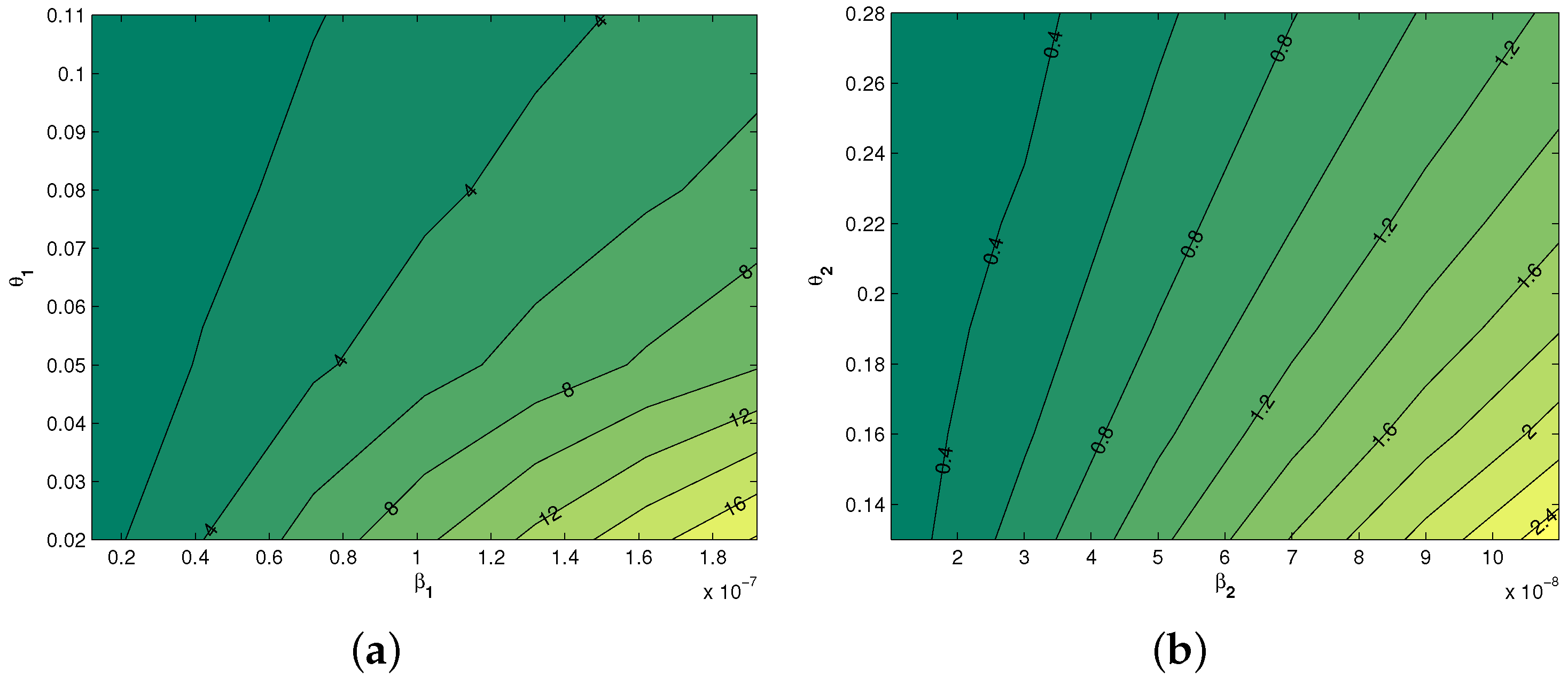
5.2. Local Sensitivity Analysis

Sensitivity analysis is needed to determine the most influential parameters in the spread of the disease. The parameter values used during the sensitivity analysis are presented in Table 2. Sensitivity analysis aims to determine the parameters that have a major influence on a model [40]. This can be known through the sensitivity index of each parameter. The parameter sensitivity index ($indm$) is given by

$$indm=\left(\frac{\partial {\mathcal{R}}_0}{\partial m}\right)\frac{m}{{\mathcal{R}}_0}$$

where m is the parameter to be analyzed. In this work, ${\mathcal{R}}_0$ is used as follows:

$${\mathcal{R}}_{01}=\frac{{\alpha }_1\Lambda \mathrm{q}+\delta {\beta }_1\Lambda }{\mu pq},{\mathcal{R}}_{02}=\frac{{\alpha }_2\Lambda \mathrm{w}+\mathcal{E}{\beta }_2\Lambda }{\mu rw}$$

The results of the parameter sensitivity index calculation can be seen in Table 3 below.

Table 3. The sensitivity index of the parameters.

Parameter	Sensitivity Index (${\mathcal{R}}_{01}$)	Parameter	Sensitivity Index (${\mathcal{R}}_{02}$)
$\Lambda$	0.9999	$\Lambda$	1
$\mu$	−1	$\mu$	−1
${\alpha }_1$	0.0031	${\alpha }_2$	0.0041
${\beta }_1$	0.9969	${\beta }_2$	0.9959
$\delta$	−0.0026	$\epsilon$	−0.0034
${\sigma }_1$	−0.0966	${\sigma }_2$	−0.1245
${\theta }_1$	−0.9	${\theta }_2$	−0.871

Based on Table 3, it can be seen that the parameters $\Lambda ,{\alpha }_1,{\beta }_1,$ ($\Lambda ,{\alpha }_2,{\beta }_2$) have positive indices showing that ${\mathcal{R}}_{01}$ (${\mathcal{R}}_{02}$) increases with the parameters. The rest of the parameters have negative sensitivity indices, which demonstrate that ${\mathcal{R}}_{01}$ and ${\mathcal{R}}_{02}$ decrease with the increase in these parameters. For example, the sensitivity index of the parameter ${\beta }_1$ is 0.9969, which mean that increasing (decreasing) ${\beta }_1$ 10% will increase (decrease) the value ${\mathcal{R}}_{01}$ by 9.969%. In contrast, increasing (decreasing) parameter ${\theta }_1$ 10% will decrease (increase) ${\mathcal{R}}_{01}$ by 9%. Similarly, the sensitivity index of parameter ${\beta }_2$ is 0.9959, which implies increasing (decreasing) ${\beta }_2$ 10% will increase (decrease) the value ${\mathcal{R}}_{02}$ by 9.959%. Thus, the increasing (decreasing) parameter ${\theta }_2$ 10% will decrease (increase) ${\mathcal{R}}_{02}$ by 8.71%.

Figure 2 depicts the impact of the parameters ${\beta }_1,{\theta }_1,{\beta }_2$, and ${\theta }_2$ on ${\mathcal{R}}_0$. Based on the contour plot in Figure 2, it can be seen that ${\mathcal{R}}_0$ is increasing with the increase of ${\beta }_1$ and ${\beta }_2,$ while it is decreased with the increase in ${\theta }_1$ and ${\theta }_2$.

Figure 2. Contour plot of (a) ${\theta }_1$ versus ${\beta }_1$ and (b) ${\theta }_2$ versus ${\beta }_2$ as a function of ${\mathcal{R}}_0.$

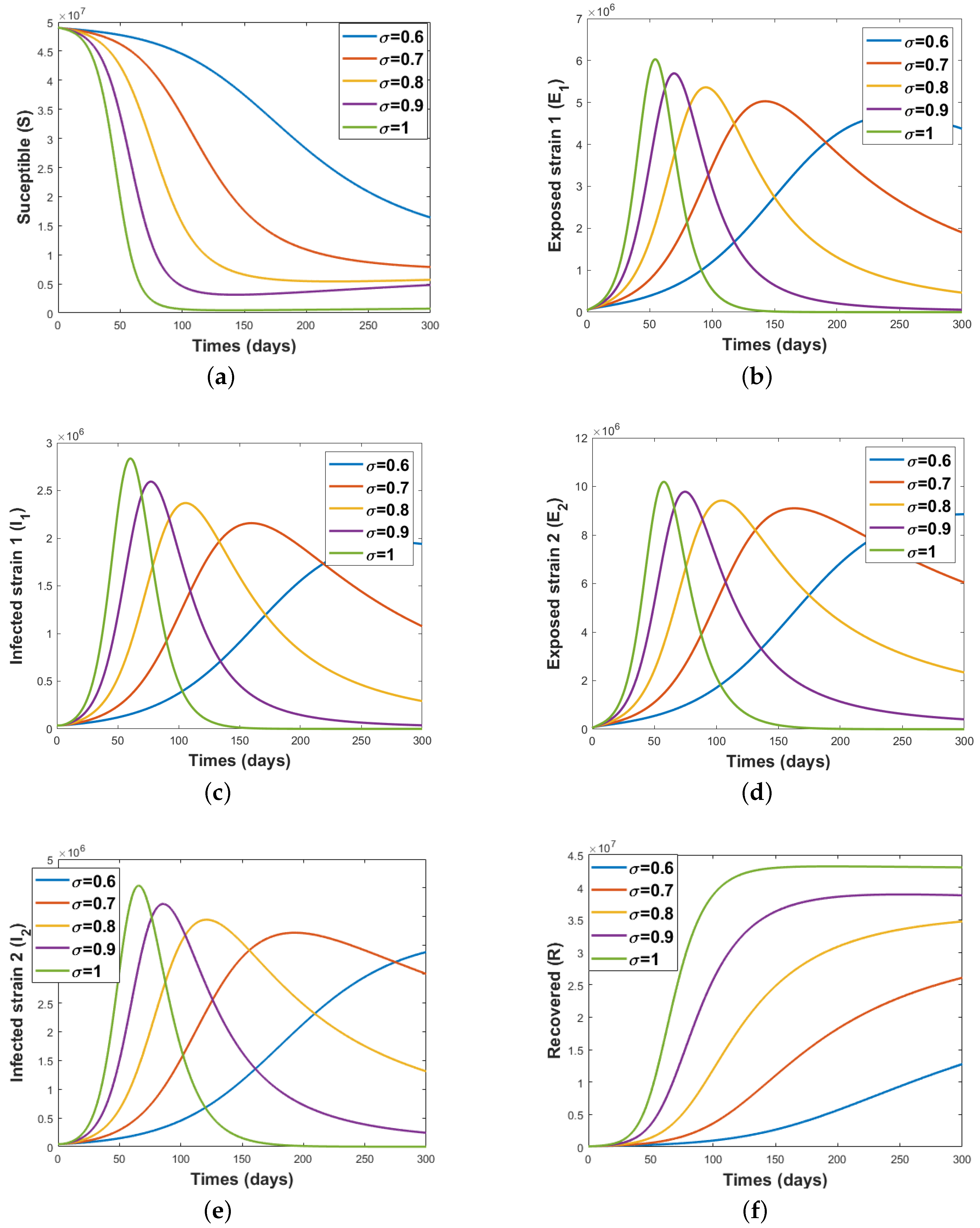
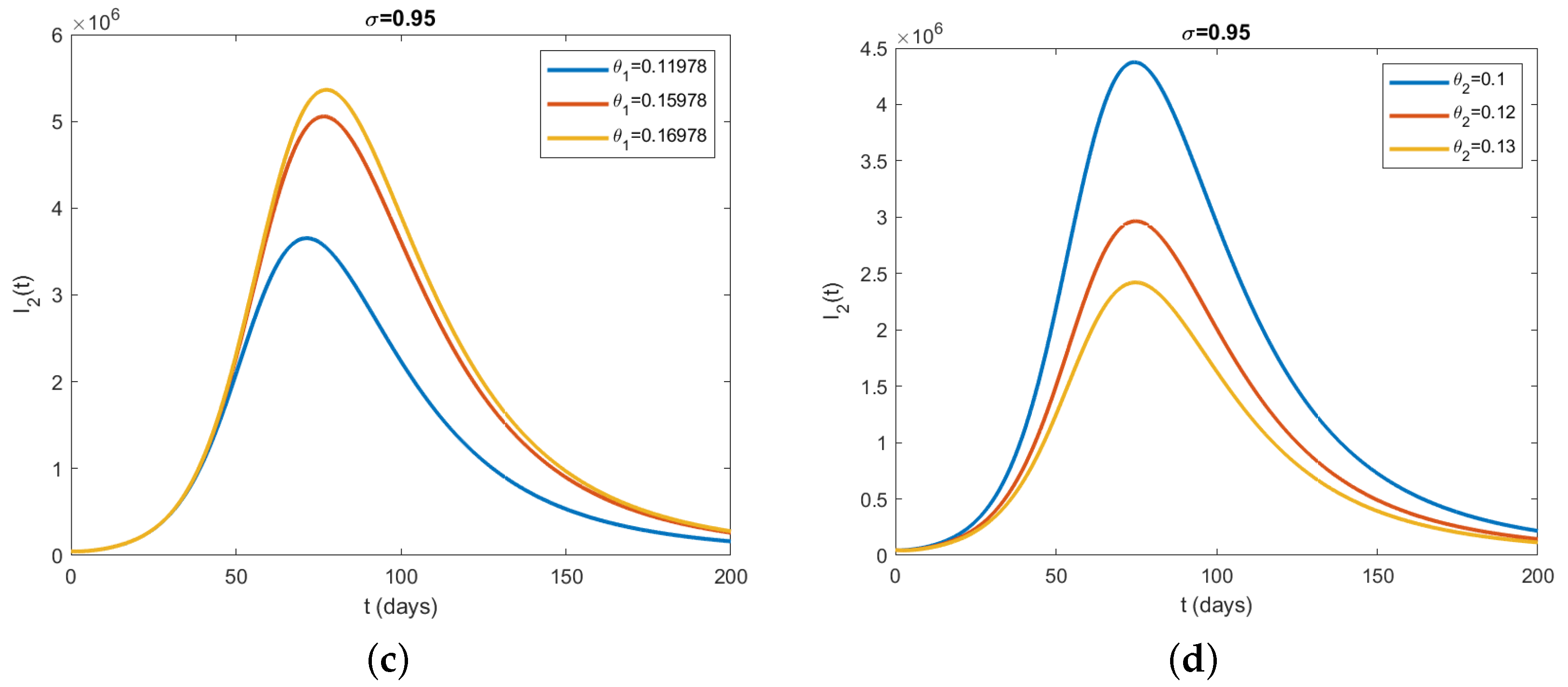
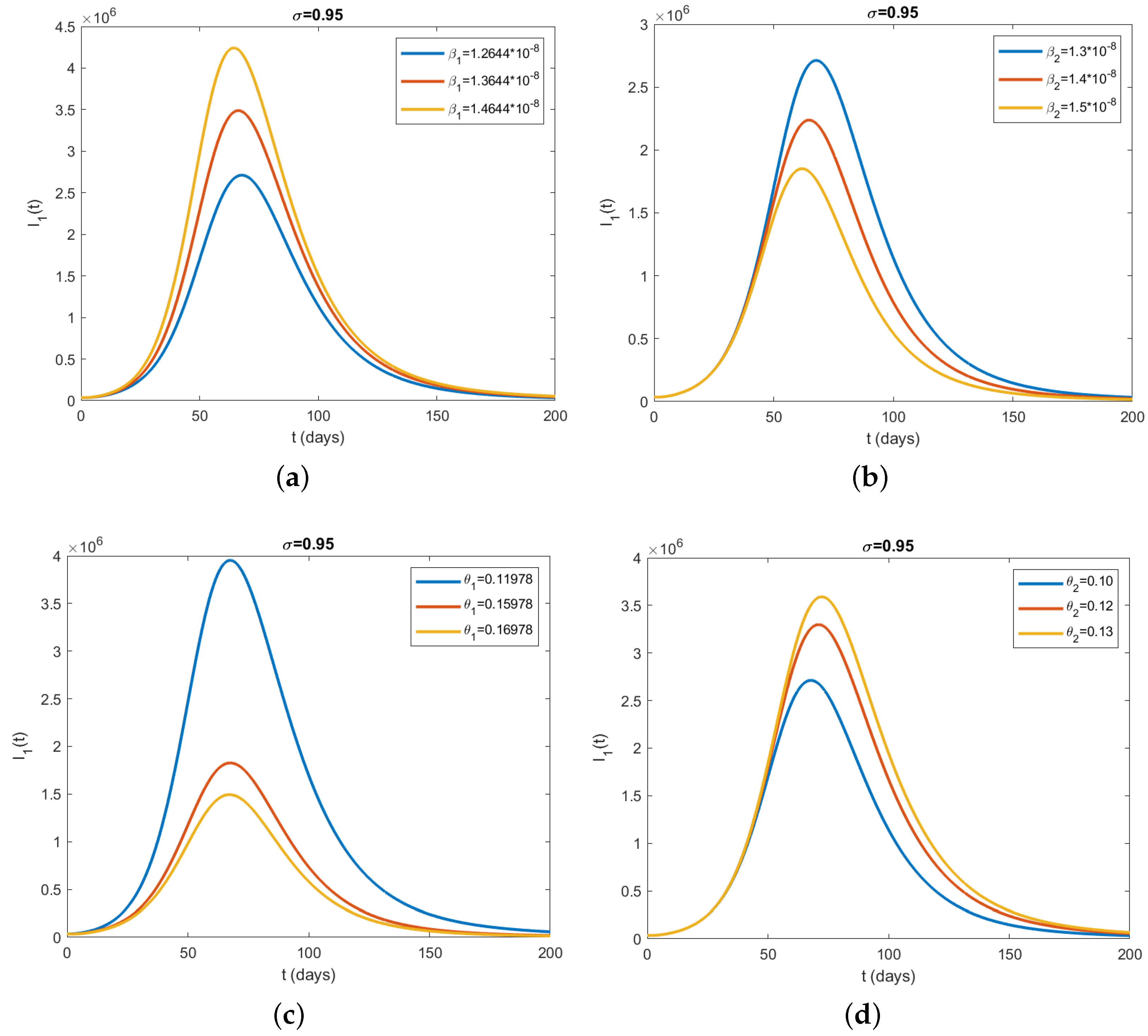
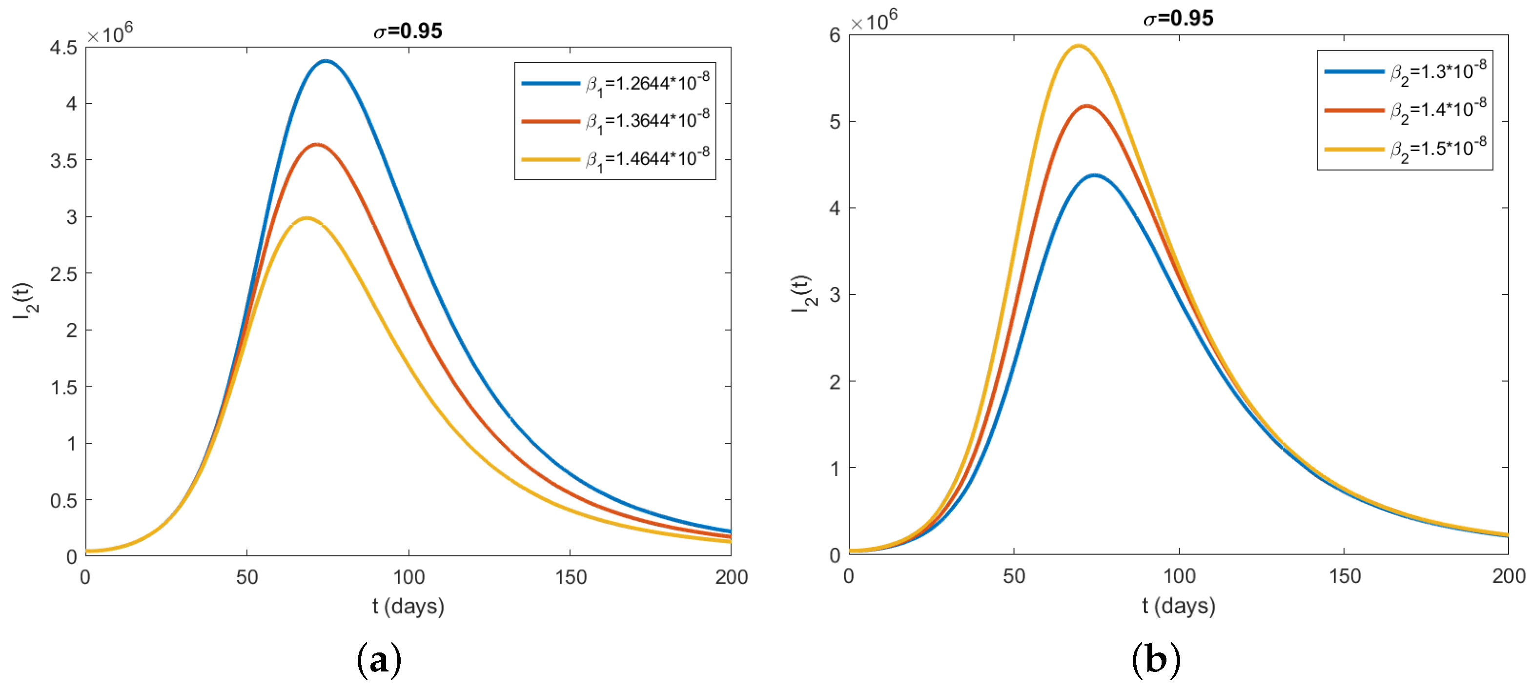
5.3. Simulation Results Using Caputo Operator

Here, we devote the numerical simulations for the fractional model (9) in the Caputo operator framework. The fractional model is solved numerically by taking the method as mentioned in [41] and the parameter values set out in Table 2.

Figure 3a characterizes susceptible individuals $\left(S\right)$ as the fractional-order derivative moves from 0.6 to the integer-order 1. From this figure, we can see that the number of susceptible individuals decreases as time increases. Naturally, this situation occurs in many epidemiological models as more individuals become infected a few weeks after the outbreak and leave the $\left(S\right)$ class. Figure 3b depicts individuals exposed to the strain 1 virus. The population of $E_1$ increases steadily as the fractional-order derivative increases toward the classical value. As it approaches the value 1, the increase becomes faster. This result is expected because more susceptible individuals contact the disease and move into the exposed class after the first few weeks of the outbreak. Figure 3c illustrates changes in the number of strain-1 infected individuals with time. The number of strain 1-infected individuals increases as the fractional-order moves toward the classical value 1. Here, the fractional order is very sensitive and drives the infection. The increase becomes faster as the fractional order becomes very close to the value 1. This is motivated by the fact that most of the exposed individuals move to the symptomatic and infectious stage a few weeks after infection. Figure 3d depicts the dynamics of individuals exposed to the strain of two viruses. As the fractional-order derivative moves toward the integer part, the population of individuals exposed to the strain two virus increases. This result is similar to the result obtained in Figure 3b, showing that the fractional order has the same effect on the exposed population regardless of the strain that the population is exposed to during the time of the infection. Similar explanations can be used to relate the similarity between the result of Figure 3c and that of Figure 3e. Figure 3f shows the changes in the number of recovered individuals from both strain one and strain two infections as the fractional order changes. The number of recovered individuals increases as the fractional-order derivative moves up toward the classical value. This steady increase originates from the fact that individuals are recovering from both strains simultaneously. The recovery of infected individuals is usually encouraged to facilitate disease containment. Increasing the fractional order is thus suggested here as we observe on the graph that the increase in the population of the R class is much faster when the fractional order is high.

Figure 3. Numerical simulation for the fractional model (9) when $\sigma =1,0.9,0.8,0.7$ and $0.6$, where (a) Susceptible individuals, (b) Exposed individuals to strain 1, (c) Infected individuals to strain 1, (d) Exposed individuals to strain 2, (e) Infected individuals to strain 2, and (f) Recovered individuals.

Figure 4a,b depict the changes that occur in the class $I_1$ when the infection rates are varied. We observe a steady increase in the number of individuals in the $I_1$ class as the strain one infection rate increases. This increase is expected because more susceptible individuals come into contact with strain one infectious individuals and contract the virus. On the other hand, increasing the strain two infection rate gives the reverse results. The steady fall in the number of individuals in class $I_1$ as the strain two infection rate increases is only an indication that increasing the strain two infection rate and leaving the strain one infection rate constant only leads to an increase in the strain two infectious population, giving time for the strain one infectious population to decrease. Figure 4c,d, on the other hand, show the effects of changes in the recovery rates on the population of class $I_1.$ In Figure 4c, we observe that when the rate of recovery from the strain one infection decreases from 0.16978 to 0.15978, there is a corresponding steady increase in the population of class $I_1.$ However, a decrease in the recovery rate from the strain one infection from 0.15978 to 0.14978 skyrockets the population of class $I_1.$ This can be explained by the fact that when the rate of recovery from the disease is very low, the prevalence of infectious individuals and hence the chances of disease spread will increase. On the contrary, an increase in the number of individuals in class $I_1$ is attained upon increasing the recovery rate from the strain two infections. The results obtained in Figure 5 can be explained in a similar fashion.

Figure 4. Effect of the model parameters (a) ${\beta }_1,\left(\mathbf{b}\right){\beta }_2,\left(\mathbf{c}\right){\theta }_1$, and (d) ${\theta }_2$ on $I_1$ individuals with fractional order $\sigma =0.95.$.

Figure 5. Effect of the model parameters (a) ${\beta }_1,\left(\mathbf{b}\right){\beta }_2,\left(\mathbf{c}\right){\theta }_1$, and (d) ${\theta }_2$ on $I_2$ individuals with fractional order $\sigma =0.95.$.

6. Conclusions

In this paper, we proposed and analyzed a fractional model of COVID-19 to track the impact of multiple stains of the SARS-CoV-2 variants during the epidemic. Mathematical analyses of the model, which envisage the positivity of solutions, basic reproduction number, and the local stability of the model, were all presented. Our results suggest that an increase in the number of infections has two variants driving the disease than only one variant. This result agrees that most countries have also experienced higher mortality and infection rates during the second or third wave than the first wave of the COVID-19 pandemic.

We acknowledge that our model is not without shortcomings. Some of the limitations are as follows: first, the model was not fitted to historic epidemiological COVID-19 data for a specific setting. Second, few of the parameter values were available in the published literature, and some were estimated where possible. Lastly, our model did not take into account the asymptomatic individuals; this may lead to not accounting for all the possible routes of infectivity in the modeling or the transmissions of the disease during the epidemic. Notwithstanding these limitations, we suggest that our findings remain valid and applicable in the control of the COVID-19 infection generated by the combination of two different strains of the SARS-CoV-2 virus if implemented by policymakers. The model can be extended by considering specific mutations of the variants at different stages and developing a multi-scale model to analyze the effects of these variants on the human population.

References

- World Health Organization (WHO). Coronavirus Disease (COVID-19) Pandemic. Available online: https://www.who.int/emergencies/diseases/novel-coronavirus-2019 (accessed on 30 April 2022).
- Thakur, V.; dan Jain, A. COVID-19-Suicides: A Global Psychological Pandemic. Brain Behav. Immun. 2020, 88, 952–953. [Google Scholar] [CrossRef] [PubMed]
- CDC. Your Health. 2020. Available online: https://www.cdc.gov/coronavirus/2019-ncov/your-health/index.html (accessed on 28 April 2022).
- World Health Organisation. COVID-19 Weekly Epidemiological Update Edition 70. Available online: https://www.who.int/docs/defaultsource/coronaviruse/situationreports/20211214_weekly_epi_update_70.pdf?sfvrsn=ad19bf83_3 (accessed on 14 May 2022).
- Guruprasad, L. Human Coronavirus Spike Protein-Host Receptor Recognition. Prog. Biophys. Mol. Biol. 2021, 161, 39–53. [Google Scholar] [CrossRef]
- WHO. Media Statement: Knowing the Risks for COVID-19. Available online: https://www.who.int/indonesia/news/detail/08-03-2020-knowing-the-risk-for-covid-19 (accessed on 29 May 2022).
- Korber, B.; Fischer, W.M.; Gnanakaran, S.; Yoon, H.; Theiler, J.; Abfalterer, W.; Hengartner, N.; Giorgi, E.E.; Bhattacharya, T.; Foley, B.; et al. Evaluating the Effects of SARS-CoV-2 Spike Mutation D614G on Transmissibility and Pathogenicity. Cell 2021, 184, 64–75. [Google Scholar]
- Korber, B.; Fischer, W.M.; Gnanakaran, S.; Yoon, H.; Theiler, J.; Abfalterer, W.; Hengartner, N.; Giorgi, E.E.; Bhattacharya, T.; Foley, B.; et al. Tracking changes in SARS-CoV-2 spike: Evidence that D614G increases infectivity of the COVID-19 virus. Cell 2020, 182, 812–827. [Google Scholar] [CrossRef] [PubMed]
- CDC. SARS-CoV-2 Variant Classifications and Definitions. Available online: https://www.cdc.gov/coronavirus/2019-ncov/variants/variant-classifications.html (accessed on 25 May 2022).
- World Health Organisation. Classification of Omicron (B.1.1.529): SARS-CoV-2 Variant of Concern. Available online: https://www.who.int/news/item/26-11-2021-classification-of-omicron-(b.1.1.529)-sars-cov-2-variant-of-concern (accessed on 25 April 2022).
- World Health Organisation. Network for Genomic Surveillance South Africa (NGS-SA). SARS-CoV-2 Sequencing. Available online: https://www.krisp.org.za/manuscripts/25Nov2021_B.1.1.529_Media.pdf (accessed on 25 September 2021).
- UK Health Security Agency. SARS-CoV-2 Variants of Concern and Variants under Investigation in England: Technical Briefing 31. Available online: https://assets.publishing.service.gov.uk/government/uploads/system/uploads/attachment_data/file/1042367/technical_briefing-31-10-december-2021.pdf (accessed on 10 March 2022).
- Wang, X.; Tang, T.; Cao, L.; Aihara, K.; Guo, Q. Inferring key epidemiological parameters and transmission dynamics of COVID-19 based on a modified SEIR model. Math. Model. Nat. Phenom. 2020, 15, 74. [Google Scholar] [CrossRef]
- Zeb, A.; Alzahrani, E.; Erturk, V.S.; Zaman, G. Mathematical model for coronavirus disease 2019 (COVID-19) containing isolation class. BioMed Res. Int. 2020, 2020, 3452402. [Google Scholar] [CrossRef]
- Aldila, D. Analyzing the impact of the media campaign and rapid testing for COVID-19 as an optimal control problem in East Java, Indonesia. Chaos Solitons Fractals 2020, 141, 109953. [Google Scholar] [CrossRef]
- Khan, M.A.; Atangana, A.; Alzahrani, E.; Fatmawati. The dynamics of COVID-19 with quarantined and isolation. Adv. Differ. Equations 2020, 1, 1–22. [Google Scholar] [CrossRef]
- Mishra, A.M.; Purohit, S.D.; Owolabi, K.M.; dan Sharma, Y.D. A Nonlinear Epidemiological Model Considering Asymtotic and Quarantine Classes for SARS-CoV-2 Virus. Chaos Solitons Fractals 2020, 138, 109953. [Google Scholar] [CrossRef]
- Aldila, D.; Ndii, M.Z.; Samiadji, B.M. Optimal control on COVID-19 eradication program in Indonesia under the effect of community awareness. Math. Biosci. Eng. 2020, 17, 6355–6389. [Google Scholar] [CrossRef]
- Alqahtani, R.T.; Ajbar, A. Study of Dynamics of a COVID-19 Model for Saudi Arabia with Vaccination Rate, Saturated Treatment Function and Saturated Incidence Rate. Mathematics 2021, 9, 3134. [Google Scholar] [CrossRef]
- Mushanyu, J.; Chukwu, W.; Nyabadza, F.; Muchatibaya, G. Modelling the potential role of super spreaders on COVID-19 transmission dynamics. Int. J. Math. Model. Numer. Optim. 2022, 12, 191–209. [Google Scholar]
- Rezapour, S.; Mohammadi, H.; Samei, M.E. SEIR epidemic model for COVID-19 transmission by Caputo derivative of fractional order. Adv. Differ. Equ. 2020, 1, 1–19. [Google Scholar] [CrossRef] [PubMed]
- Naik, P.A.; Yavuz, M.; Qureshi, S.; Zu, J.; Townley, S. Modeling and analysis of COVID-19 epidemics with treatment in fractional derivatives using real data from Pakistan. Eur. Phys. J. Plus 2020, 135, 795. [Google Scholar] [CrossRef] [PubMed]
- Boudaoui, A.; El hadj Moussa, Y.; Hammouch, Z.; Ullah, S. A fractional-order model describing the dynamics of the novel coronavirus (COVID-19) with nonsingular kernel. Chaos Solitons Fractals 2021, 146, 110859. [Google Scholar] [CrossRef]
- Chukwu, C.W.; Fatmawati. Modelling fractional-order dynamics of COVID-19 with environmental transmission and vaccination: A case study of Indonesia. AIMS Math. 2022, 7, 4416–4438. [Google Scholar] [CrossRef]
- Li, X.P.; DarAssi, M.H.; Khan, M.A.; Chukwu, C.W.; Alshahrani, M.Y.; Al Shahrani, M.; Riaz, M.B. Assessing the potential impact of COVID-19 Omicron variant: Insight through a fractional piecewise model. Results Phys. 2022, 38, 105652. [Google Scholar] [CrossRef]
- Bonyah, E.; Juga, M.; Fatmawati. Fractional dynamics of coronavirus with comorbidity via Caputo-Fabrizio derivative. Commun. Math. Biol. Neurosci. 2022, 2022, 12. [Google Scholar]
- Gao, W.; Veeresha, P.; Cattani, C.; Baishya, C.; Baskonus, H.M. Modified Predictor–Corrector Method for the Numerical Solution of a Fractional-Order SIR Model with 2019-nCoV. Fractal Fract. 2022, 6, 92. [Google Scholar] [CrossRef]
- Qureshi, S.; Bonyah, E.; Shaikh, A.A. Classical and contemporary fractional operators for modeling diarrhea transmission dynamics under real statistical data. Phys. Stat. Mech. Its Appl. 2022, 535, 122496. [Google Scholar] [CrossRef]
- Bonyah, E.; Juga, M.L.; Chukwu, C.W.; Fatmawati. A fractional order dengue fever model in the context of protected travelers. Alex. Eng. J. 2022, 61, 927–936. [Google Scholar] [CrossRef]
- Bonyah, E.; Chukwu, C.W.; Juga, M.; Fatmawati. Modeling fractional order dynamics of Syphilis via Mittag-Leffler law. AIMS Math. 2021, 6, 8367–8389. [Google Scholar] [CrossRef]
- Ade León, U.A.P.; Avila-Vales, E.; Huang, K.L. Modeling COVID-19 dynamic using a two-strain model with vaccination. Chaos Solitons Fractals 2022, 157, 111927. [Google Scholar] [CrossRef] [PubMed]
- Arruda, E.F.; Das, S.S.; Dias, C.M.; Pastore, D.H. Modelling and optimal control of multi strain epidemics, with application to COVID-19. PLoS ONE 2021, 16, e0257512. [Google Scholar] [CrossRef] [PubMed]
- Li, R.; Li, Y.; Zou, Z.; Liu, Y.; Li, X.; Zhuang, G.; Shen, M.; Zhang, L. Evaluating the impact of SARS-CoV-2 variants on the COVID-19 epidemic and social restoration in the United States: A mathematical modelling study. Front. Public Health 2021, 9, 2067. [Google Scholar] [CrossRef]
- González-Parra, G.; Arenas, A.J. Qualitative analysis of a mathematical model with presymptomatic individuals and two SARS-CoV-2 variants. Comput. Appl. Math. 2021, 40, 1–25. [Google Scholar] [CrossRef]
- Layton, A.T.; Sadria, M. Understanding the dynamics of SARS-CoV-2 variants of concern in Ontario, Canada: A modeling study. Sci. Rep. 2022, 12, 1–16. [Google Scholar] [CrossRef]
- Podlubny, I. Fractional Differential Equations: An Introduction to Fractional Derivatives, Fractional Differential Equations, to Methods of Their Solution and Some of Their Applications; Academic Press: San Diego, CA, USA, 1999. [Google Scholar]
- Vargas-De-Le´on, C. Volterra-type Lyapunov functions for fractional-order epidemic systems. Commun. Nonlinear Sci. Numer. Simul. 2015, 24, 75–85. [Google Scholar] [CrossRef]
- Van den Driessche, P.; Watmough, J. Reproduction numbers and sub-threshold endemic equilibria for compartmental models of disease transmission. Bull. Math. Biol. 2008, 70, 29–48. [Google Scholar] [CrossRef]
- Ahmed, E.; El-Sayed, A.M.A.; El-Saka, H.A.A. On some Routh-Hurwitz conditions for fractional order differential equations and their applications in Lorenz, Rossler, Chua and Chen systems. Phys. Lett. 2006, 1, 1–4. [Google Scholar] [CrossRef]
- Chitnis, N.; Hyman, J.M.; Cushing, J.M. Determining important parameters in the spread of malaria through the sensitivity analysis of a mathematical model. Bull. Math. Biol. 2008, 70, 1272–1296. [Google Scholar] [CrossRef] [PubMed]
- Diethelm, K.; Freed, A.D. The FracPECE subroutine for the numerical solution of differential equations of fractional order. Forsch. Und Wiss. Rechn. 1999, 57–71. [Google Scholar]
Publisher’s Note: MDPI stays neutral with regard to jurisdictional claims in published maps and institutional affiliations. |
© 2022 by the authors. Licensee MDPI, Basel, Switzerland. This article is an open access article distributed under the terms and conditions of the Creative Commons Attribution (CC BY) license (https://creativecommons.org/licenses/by/4.0/).