Article

Threshold Dynamics and the Density Function of the Stochastic Coronavirus Epidemic Model

School of Science, China University of Petroleum (East China), Qingdao 266580, China
*
Author to whom correspondence should be addressed.
Fractal Fract. 2022, 6(5), 245; https://doi.org/10.3390/fractalfract6050245
Submission received: 2 April 2022 / Revised: 27 April 2022 / Accepted: 27 April 2022 / Published: 29 April 2022
(This article belongs to the Special Issue Stochastic Modeling in Biological System)

Abstract

:
Since November 2019, each country in the world has been affected by COVID-19, which has claimed more than four million lives. As an infectious disease, COVID-19 has a stronger transmission power and faster propagation speed. In fact, environmental noise is an inevitable important factor in the real world. This paper mainly gives a new random infectious disease system under infection rate environmental noise. We give the existence and uniqueness of the solution of the system and discuss the ergodic stationary distribution and the extinction conditions of the system. The probability density function of the stochastic system is studied. Some digital simulations are used to demonstrate the probability density function and the extinction of the system.

1. Introduction

So far, infectious diseases have become one of the important factors endangering human health. Medical research shows that there are three outcomes of any infectious disease: the first is that the infectious virus is eliminated by human drugs; the second is that the virus exists only in a small area, such as Ebola, SARS (severe acute respiratory syndrome), and so on; the third is the long-term coexistence of viruses and humans, such as influenza, AIDS (acquired immunodeficiency syndrome), and so on [1].
In order to describe the dynamic behavior of the epidemic, mathematical modeling is considered to be an important tool [2]. According to the occurrence, transmission, and development law of infectious disease in the population, Mathematicians and ecologists have established several epidemic models to study and control various epidemics [3,4,5]. The authors gave the dynamics and stationary distribution of the hepatitis E model. Meanwhile, the authors obtained the optimal control analysis and the Atangana–Baleanu derivative for the dynamical analysis of the hepatitis E model in [6]. Through the qualitative analysis and numerical simulation of the dynamic behavior of the infectious disease model [7], the authors gave an exact expression of the probability density function of the stochastic model SVI (susceptible, vaccinated, infectious) around the unique endemic equilibrium of the deterministic system by solving the corresponding Fokker–Planck equation, which is guaranteed by a new critical value R 0 s in [8], and other models, such as SIR (susceptible, infectious, recovered), SIRS (susceptible, infectious, recovered, susceptible), SEIR (susceptible, exposed, infectious, recovered), etc. [9,10].
Since November 2019, the world has been enveloped in COVID-19 (coronavirus disease 2019). As a contagious virus, COVID-19 is highly infectious [11]. Since April 2021, only half a year, the number of newly confirmed cases in the world has increased by 100 million [12]. At the same time, Griffin B.D., etc. [13], found that the new coronavirus could infect and spread among North American deer rats, which has increased the difficulty in controlling COVID-19. Many countries are working hard to prevent the spread of COVID-19. Mathematicians use simulated mathematical models to predict the future behavior of coronavirus disease transmission in 2019. So far, several typical 2019 coronavirus disease transmission models have been proposed and are being used in some decisions. Recently, people have grasped valuable inferences through mathematical modeling and obtained in-depth understanding of the novel coronavirus (COVID-19) [14]. A. Atangana confirmed the effect of lockdown as a possible adequate measure to help flatten the curve of deaths and infections with the epidemic model as follows: [15]:
d S ( t ) = [ Λ β S ( t ) D ( t ) N ( δ + μ ) S ( t ) + η R ( t ) ] d t , d C ( t ) = [ ( β S ( t ) D ( t ) N + δ S ( t ) ( β + μ + π ) C ( t ) ] d t , d I ( t ) = [ δ ( 1 θ ) S ( t ) + π C ( t ) ( τ + μ + σ ) I ( t ) ] d t , d R ( t ) = [ β C ( t ) + τ I ( t ) ( μ + η ) R ( t ) ] d t , d D ( t ) = [ σ I ( t ) ] d t ,
where the parameters are in Table 1.
However, in the real world, due to the influence of various factors, such as the environment, a random model is constructed by random components with some distribution. Through the addition of some white noise, these distributions may reflect the uncertainty of the input content or random process [16]. Meanwhile, the quarantined measures play a very important role in fighting and preventing the increase in COVID-19. The authors found that the dynamic system with the external source was more reliable than the suspected people travelling, and that the rate of isolation is extremely important for controlling the increase in the cumulative confirmed people of COVID-2019 [17]. The authors in [18] put forward the stochastic coronavirus epidemic model with the parameter disturbance by the natural mortality rate by translating the quarantined factor as follows:
d S ( t ) = [ Λ β S ( t ) I ( t ) N μ 0 S ( t ) ] d t + η 1 S ( t ) d B 1 ( t ) , d I ( t ) = [ ( β S ( t ) I ( t ) N ( γ 1 + μ 1 + μ 0 ) I ( t ) + σ Q ( t ) ] d t + η 2 I ( t ) d B 2 ( t ) , d Q ( t ) = [ γ 1 I ( t ) ( μ 0 + μ + σ ) Q ( t ) ] d t + η 3 Q ( t ) d B 3 ( t ) ,
where the definitions of the parameters are in Table 2 and N = S ( t ) + I ( t ) + Q ( t ) .
In the system (2), the important role of isolation in COVID-19 is pointed out, and the stable distribution of the model under extinction conditions is obtained. However, in the real world, according to the COVID-19 data in Pakistan [19], the disturbance of the infection rate coefficient plays a very important role in the spread of COVID-19. Meanwhile, vaccination and isolation measures can also affect the infection rate. In the present paper, we give the stochastic coronavirus epidemic model with the stochastic disturbance of the infection rate coefficient. The system is the following:
d S ( t ) = [ Λ β S ( t ) I ( t ) N μ 0 S ( t ) ] d t η S ( t ) I ( t ) N d B ( t ) , d I ( t ) = [ ( β S ( t ) I ( t ) N ( γ 1 + μ 1 + μ 0 ) I ( t ) + σ Q ( t ) ] d t + η S ( t ) I ( t ) N d B ( t ) , d Q ( t ) = [ γ 1 I ( t ) ( μ 0 + μ + σ ) Q ( t ) ] d t ,
The main composition of the present paper is as follows. The second section gives the basic lemma and basic concepts of this paper. The existence and uniqueness of the global positive solution of the system (3) are obtained in the third section, and the fourth section gives the ergodic stationary distribution of the system (3). In order to better understand the degree of control of the virus, we consider the extinction condition of the system (3) in the fifth section. Meanwhile, in the sixth section, the probability density function of the system (3) is given to understand the trend of the coronavirus viruses in the system (3). In the last section, by numerical simulation, two examples give the extinction, long-term persistence, and the probability density function with the corresponding conditions.

2. Preliminaries

We give some basic conceptions as in [3,5,16,20]. Suppose ( Ω , F , { F t } t 0 , P ) is a complete probability space with a filtration { F t } t 0 ; we define R + 3 = { x R 3 : x i > 0 for   all 1 i 3 } and R ¯ + 3 = { x R 3 : x i 0 for   all 1 i 3 } . In addition, if f ( t ) is an integral function on t [ 0 , ) , we define f μ = s u p { f ( t ) t 0 } , f l = i n f { f ( t ) t 0 } . In the following, we give the It o ^ s formula.
Lemma 1 
([3]). Let x ( t ) be an It o ^ process with the stochastic differential
d x ( t ) = f ( t ) d t + g ( t ) d B t , f o r t t 0 ,
where f L 1 ( R + , R ) and g L 1 ( R + , R ) . Let V C 2 , 1 ( R × R + , R ) . Then, V ( x ( t ) , t ) is again an It o ^ process with the stochastic differential given by
d V ( x ( t ) , t ) = [ V t ( x ( t ) , t ) + V x ( x ( t ) , t ) f ( t ) + 1 2 V x x ( x ( t ) , t ) g 2 ( t ) ] d t + V x ( x ( t ) , t ) g ( t ) d B t a . s .
Firstly, we consider the general three-dimensional stochastic differential equation
d x ( t ) = f ( x ( t ) , t ) d t + g ( x ( t ) , t ) d B ( t ) , f o r t t 0
with initial value x ( t 0 ) = x 0 R 3 , where B ( t ) denotes three-dimensional standard Brownian motion defined on the above probability space ( Ω , Γ , { Γ t } t 0 , P ) . Define the differential operator L by Mao [3] as
L = t + Σ f i ( x , t ) x i + 1 2 Σ [ g T ( x , t ) g ( x , t ) ] i j 2 x i x j .
If L acts on a function V C 2 , 1 ( R 3 × R ¯ + ; R ¯ + ) , where R ¯ + = { x R : x 0 } , then
L V ( x , t ) = V t ( x , t ) + V x ( x , t ) + 1 2 t r a c [ g T ( x , t ) V x x ( x , t ) g ( x , t ) ] ,
where V t = V t , V x = ( V x 1 , , V x 3 ) and V x x = ( 2 V x i x j ) 3 × 3 .
By Lemma 1, we obtain
d V ( x ( t ) , t ) = L V ( x ( t ) , t ) d t + V x ( x ( t ) , t ) g ( x ( t ) , t ) d B ( t ) .
The diffusion matrix is defined as follows:
A ( x ) = ( a i j ( x ) ) , a i j = r = 1 3 g r i ( x ) g r j ( x ) , 1 i , j 3 .

3. Existence and Uniqueness of the Global Positive Solution

The problem where the solution is global and positive is important in studying the dynamical behavior of the system (3). The coefficients of the system (3) are not the linear growth, and the solutions of the system (3) may explode at a fixed time. The main theorem is as follows.
Theorem 2. 
There is a unique positive solution ( S ( t ) , I ( t ) , Q ( t ) ) of system (3) on t 0 by the initial value ( S ( 0 ) , I ( 0 ) , Q ( 0 ) ) R + 3 , and the solution ( S ( t ) , I ( t ) , Q ( t ) ) R + 3 for all t 0 almost surely (a.s.).
Proof. 
Based on [5], we obtain the fact that there is a unique solution ( x ( t ) , y ( t ) , z ( t ) , w ( t ) ) on [ 0 , τ 0 ) for the reason that the coefficients of the system (3) are the locally Lipschitz continuous, where τ 0 is an explosion time. We can obtain the fact that the local solution is global when τ 0 = a.s. By the definitions in [3], we define a fundamental C 2 -function U : R + 3 R ¯ + , which is
U ( S , I , Q ) = ( S ( t ) 1 ln S ( t ) ) + a ( I ( t ) 1 β ln I ( t ) ) + b ( Q ( t ) 1 ln Q ( t ) ) ,
where a , b are positive constants, which will be determined in the following text. The non-negativity of the function U can be seen from x 1 ln x 0 for any x > 0 .
Applying It o ^ s formula [3], we obtain
d U ( S , I , Q ) = L U d t + η ( S ( t ) 1 ) I ( t ) N 2 d B ( t ) η ( I ( t ) 1 ) S ( t ) N 2 d B ( t ) ,
where
L U = ( 1 1 S ) ( Λ β S I N μ 0 S ) η 2 2 ( I N ) 2 + ( 1 1 I ) [ ( β S I N ( γ 1 + μ 1 + μ 0 ) I + σ Q ] + η 2 2 ( S N ) 2 + ( 1 1 Q ) [ γ 1 I ( μ 0 + μ + σ ) Q ] = Λ β S I N μ 0 S Λ S + β I N + μ 0 ( μ 0 + μ 1 + γ 1 ) I + β S I N + σ Q β S N + ( μ 0 + μ 1 + γ 1 ) σ Q I + γ 1 I ( μ 0 + μ + σ ) Q γ 1 I Q + ( μ 0 + μ + σ ) η 2 2 ( I N ) 2 + η 2 2 ( S N ) 2 Λ μ 0 S Λ S + β + μ 0 ( μ 0 + μ 1 + γ 1 ) I + σ Q + ( μ 0 + μ 1 + γ 1 ) ( μ 0 + μ + σ ) Q σ Q I + γ 1 I γ 1 I Q + ( μ 0 + μ + σ ) + η 2 2 Λ μ 0 S Λ S + β + μ 0 + ( μ 0 + μ 1 + γ 1 ) σ Q I γ 1 I Q + ( μ 0 + μ + σ ) + η 2 2 Λ + β + 3 μ 0 + μ 1 + γ 1 + μ + σ 2 μ 0 Λ 2 σ γ 1 + η 2 2 = ( Λ μ 0 ) 2 + ( σ γ 1 ) 2 + β + 2 μ 0 + μ 1 + μ + η 2 2 ,
Then, we can obtain
L U ( Λ μ 0 ) 2 + ( σ γ 1 ) 2 + β + 2 μ 0 + μ 1 + μ + η 2 2 : = K ,
where K is a positive constant. The remainder of the proof is similar to Theorem 3.1 in Mao [5]. Hence, we omit it here. □

4. Ergodic Stationary Distribution of the Stochastic Coronavirus Epidemic Model

In this section, the existence of ergodic stationary components of the system (3) is given. Firstly, we define R 0 * as a stochastic reproductive ratio of the system (3), such as
R 0 * = μ 0 β σ γ 1 ( μ 0 + 1 2 η 2 ) ( γ 1 + μ 1 + μ 0 + 1 2 η 2 ) 2 ( μ 0 + μ + σ ) ,
which is equal to β σ γ 1 ( γ 1 + μ 1 + μ 0 ) 2 ( μ 0 + μ + σ ) when η = 0 [3]. The following is a known result.
Lemma 3 
([3,5]). The Markov process X ( t ) has a stationary distribution μ ( · ) if there exists a bounded domain U E l with regular boundary Γ and
  • (B.1) there is a positive number M such that i , j = 1 l a i j ( x ) ξ i ξ j M | ξ | 2 , x U , ξ R l ;
  • (B.2) there exists a nonnegative C 2 function V such that L V is negative for any E l \ U . Then,
    P x lim T 1 T 0 T f ( X ( t ) ) d t = E l f ( x ) μ ( d x ) = 1 ,
for all x E l , where f ( · ) is a function integrable with respect to the measure μ.
Theorem 4. 
When R 0 * > 1 , for the solution ( S ( t ) , I ( t ) , Q ( t ) ) of the system (3), there exists an ergodic unique stationary distribution.
Proof. 
We construct a C 2 -function V ˜ : R + 3 R as follows:
V ˜ = N ( t ) c 1 ln S ( t ) c 2 ln I ( t ) c 3 ln Q ( t ) .
Applying It o ^ s formula [3], we obtain
L V ˜ = ( Λ μ 0 N μ 1 I μ Q ) + c 1 [ Λ S + β I N + μ 0 + 1 2 ( η I N ) 2 ] + c 2 [ β S N + ( γ 1 + μ 1 + μ 0 ) σ Q I + 1 2 ( η S N ) 2 ] + c 3 [ γ 1 I Q + ( μ 0 + μ + σ ) ] = c 1 β I N + [ μ 0 N c 1 Λ S c 2 β S N c 2 σ Q I c 3 γ 1 I Q ] + c 1 ( μ 0 + 1 2 η 2 ) + c 2 ( γ 1 + μ 1 + μ 0 + 1 2 η 2 ) + c 3 ( μ 0 + μ + σ ) + Λ μ 1 I μ Q c 1 β I N 5 ( μ 0 c 1 c 2 2 c 3 β σ Λ γ 1 ) 1 5 + c 1 ( μ 0 + 1 2 η 2 ) + c 2 ( γ 1 + μ 1 + μ 0 + 1 2 η 2 ) + c 3 ( μ 0 + μ + σ ) + 2 Λ c 1 β I N 5 Λ [ ( R 0 * ) 1 5 1 ] ,
and R 0 * = μ 0 β σ γ 1 ( μ 0 + 1 2 η 2 ) ( γ 1 + μ 1 + μ 0 + 1 2 η 2 ) 2 ( μ 0 + μ + σ ) . We choose c 1 = Λ μ 0 + 1 2 η 2 , c 2 = Λ γ 1 + μ 1 + μ 0 + 1 2 η 2 , c 3 = Λ μ 0 + μ + σ .
When R 0 * > 1 , we suppose
V ¯ = M V ˜ ln S ( t ) ln I ( t ) ln Q ( t ) + N ( t ) ,
and V : = V ¯ ( S , I , Q ) V ¯ ( S 0 , I 0 , Q 0 ) .
Applying It o ^ s formula to V, we obtain
L V = M L V ˜ L ln S ( t ) L ln I ( t ) L ln Q ( t ) + L N ( t ) = 5 Λ M [ ( R 0 * ) 1 5 1 ] + c 1 M β I N + ( Λ S + β I N + μ 0 + 1 2 η 2 + [ β S N + ( γ 1 + μ 1 + μ 0 ) σ Q I 1 2 η 2 ] + [ γ 1 I Q + ( μ 0 + μ + σ ) ] + Λ μ 0 N μ 1 I μ Q 5 Λ M [ ( R 0 * ) 1 5 1 ] + ( c 1 M + 1 ) β Λ S σ Q I γ 1 I Q β S N + 3 μ 0 + γ 1 + μ 1 + μ + σ + Λ μ 0 N μ 1 I μ Q ( c 1 M + 1 ) β + 3 μ 0 + γ 1 + μ 1 + μ + σ + Λ Λ S σ Q I γ 1 I Q μ 0 S ( μ 1 + μ 0 ) I ( μ + μ 0 ) Q .
Define
f 1 ( S ) = ( c 1 M + 1 ) β + 3 μ 0 + γ 1 + μ 1 + μ + σ + Λ Λ S μ 0 S ,
f 2 ( I ) = σ Q I ( μ 1 + μ 0 ) I ,
f 3 ( Q ) = γ 1 I Q ( μ + μ 0 ) Q .
We can divide R + 3 \ D ε into the following six domains:
D 1 = { ( S , I , Q ) R + 3 : 0 < S < ε } ; D 2 = { ( S , I , Q ) R + 3 : S > 1 ε } ;
D 3 = { ( S , I , Q ) R + 3 : 0 < I < ε } ; D 4 = { ( S , I , Q ) R + 3 : I > 1 ε } ;
D 5 = { ( S , I , Q ) R + 3 : Q < ε 2 , I > ε } ; D 6 = { ( S , I , Q ) R + 3 : Q > 1 ε } ;
Clearly, D ε = j = 1 6 D j . In the following text, we will show that L V ( S , I , Q ) 1 on R + 3 \ D ε .
Case 1. If ( S , I , Q ) D 1 D 2 , one can choose
M < μ 0 + 1 2 η 2 Λ ,
and
L V ( S , I , Q ) 3 μ 0 + γ 1 + μ 1 + μ + σ + Λ Λ S μ 0 S 2 ;
Case 2. If ( S , I , Q ) D 3 D 4 ,
L V ( S , I , Q ) ( c 1 M + 1 ) β + 3 μ 0 + γ 1 + μ 1 + μ + σ + Λ + f 2 ( I ) 2 ;
Case 3. If ( S , I , Q ) D 5 D 6 ,
L V ( S , I , Q ) ( c 1 M + 1 ) β + 3 μ 0 + γ 1 + μ 1 + μ + σ + Λ + f 3 ( Q ) 2 ;
therefore, for all ( S , I , Q ) ) R + 3 \ D ε , L V ( S , I , Q ) ) 1 , which indicates that assumption ( B . 2 ) holds.
We can know that the system (3) is ergodic and has a unique stationary distribution. This completes the proof. □

5. Extinction of the Stochastic Coronavirus Epidemic Model

It is a very important topic to consider the dynamic behavior of the epidemic virus to obtain the conditions for the virus to be eliminated in a long time. We mainly discuss the extinction conditions of the system (3). According to the results in [10], we can obtain the following lemma.
Lemma 5. 
For any initial value, the solution of stochastic model satisfies
lim t ln x ( t ) t 0 , lim t ln y ( t ) t 0 , lim t ln z ( t ) t 0 , lim t ln w ( t ) t 0 a . s .
lim t x ( t ) + y ( t ) + z ( t ) + w ( t ) t = 0 , a . s . .
Moreover,
lim t 0 1 t 0 t x ( m ) d B 1 ( m ) = 0 , lim t 0 1 t 0 t y ( m ) d B 2 ( m ) = 0 , lim t 0 1 t 0 t z ( m ) d B 3 ( m ) = 0 a . s . .
Theorem 6. 
Let ( S ( t ) , I ( t ) , Q ( t ) ) be the solution of system (3) with any initial value ( S ( 0 ) , I ( 0 ) , Q ( 0 ) ) R + 3 . If R 0 S < 1 , then the solution ( S ( t ) , I ( t ) , Q ( t ) ) of system (3) satisfies
lim sup t ln I ( t ) t 1 μ 0 + γ 1 + μ 1 + μ + σ ( R 0 S 1 ) < 0 a . s . ,
where R 0 S = β 2 η 2 ( μ 0 + γ 1 + μ 1 + μ + σ ) . Namely, the disease will be eradicated in the long term.
Proof. 
Applying It o ^ s formula to ln I ( t ) , we obtain
d ln I ( t ) = d I ( t ) I ( t ) = ( β S N ( γ 1 + μ 1 + μ 0 ) + σ Q I ) d t 1 2 ( η S N ) 2 d t η S N d B ( t ) [ β S N 1 2 ( η S N ) 2 ( γ 1 + μ 1 + μ 0 ) + σ ] d t η S N d B ( t ) { η 2 2 [ ( S N ) 2 2 β η 2 S N + ( β η 2 ) 2 ( β η 2 ) 2 ] ( γ 1 + μ 1 + μ 0 ) + σ } d t η S N d B ( t ) [ β 2 2 η 2 ( γ 1 + μ 1 + μ 0 σ ) ] d t η S N d B ( t ) .
Integrating the above formula from 0 to t on both sides, we obtain
ln I ( t ) ln I ( 0 ) 0 t [ β 2 2 η 2 ( γ 1 + μ 1 + μ 0 σ ) ] d s 0 t η S N d B ( t ) .
According to the strong law of large numbers [20], we have
lim t 0 1 t 0 t η S N d B ( t ) = 0 a . s . .
and we can obtain
lim sup t ln I ( t ) t 0 t [ β 2 η 4 ( γ 1 + μ 1 + μ 0 σ ) ] d s β 2 η 4 ( γ 1 + μ 1 + μ 0 σ ) = ( γ 1 + μ 1 + μ 0 σ ) ( β 2 η 4 ( γ 1 + μ 1 + μ 0 σ ) 1 ) < 0 a . s . .
We choose R 0 S = β 2 η 2 ( μ 0 + γ 1 + μ 1 + μ + σ ) < 1 , which is equal to η > ( η 2 μ 0 + γ 1 + μ 1 + μ + σ ) 1 4 .
Therefore, the above indicates that
lim t I ( t ) = 0 a . s . .
and we can obtain the fact that the viral will be eradicated, which completes the proof. □

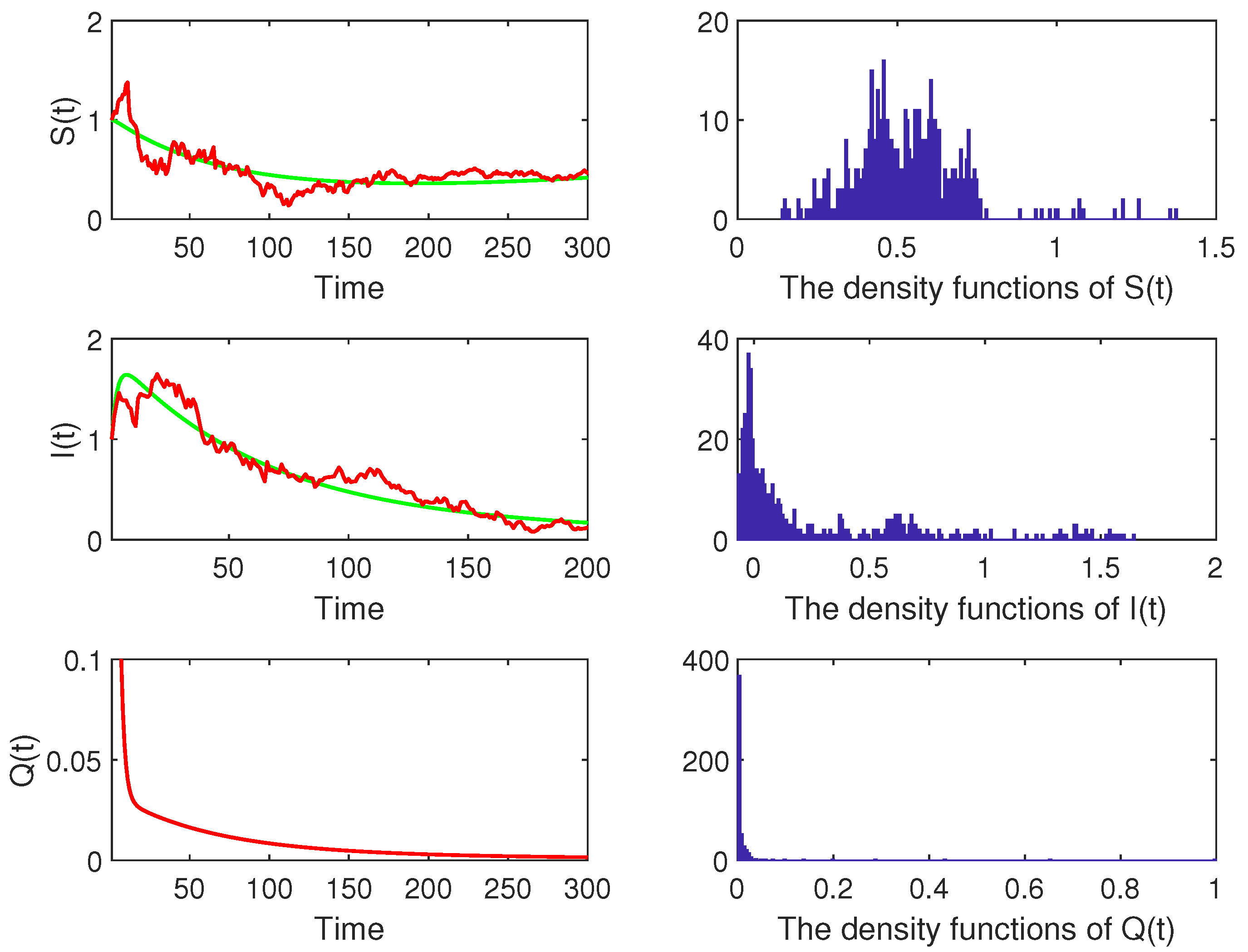
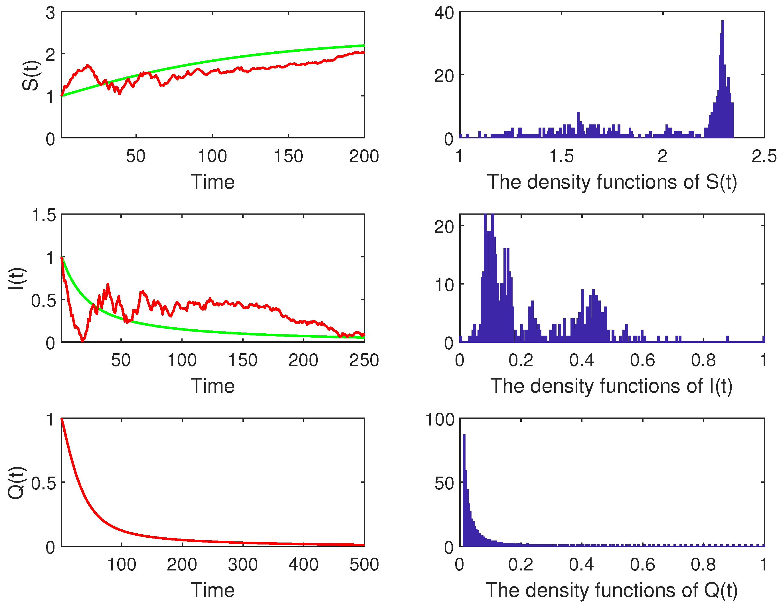
6. The Probability Density Function of the Stochastic Coronavirus Epidemic Model

Let N = S + I + Q ; we can transfer system (3) into the following system:
d S ( t ) = [ Λ β S ( t ) ( N ( t ) S ( t ) Q ( t ) ) N μ 0 S ( t ) ] d t η S ( t ) ( N ( t ) S ( t ) Q ( t ) ) N d B ( t ) d Q ( t ) = ( γ 1 N ( t ) γ 1 S ( t ) ( γ 1 + μ 0 + μ + σ ) Q ( t ) ) d t d N ( t ) = [ Λ ( μ 1 + μ 0 ) N ( t ) + μ 1 S ( μ 1 μ ) Q ( t ) ] d t .
Hence, we can consider the probability density function of system (17) in place of system (3).
Theorem 7. 
We consider the condition that R 0 * > 1 , for any initial value ( S ( 0 ) , Q ( 0 ) , N ( 0 ) ) R + 3 ; then, the solution ( S ( t ) , Q ( t ) , N ( t ) ) of system (3) with a weak kernel will have a normal probability density function Φ ( S ( t ) , Q ( t ) , N ( t ) ) around ( S * , Q * , N * ) , which is given by
Φ ( S ( t ) , Q ( t ) , N ( t ) ) = ( 2 π ) 3 2 Σ 1 2 ( S ( t ) , Q ( t ) , N ( t ) ) Σ 1 ( S ( t ) , Q ( t ) , N ( t ) ) T ,
where Σ is a positive definite matrix and satisfies
Σ = a 2 2 ( a 1 a 2 a 3 ) 0 1 2 ( a 1 a 2 a 3 ) 0 1 2 ( a 1 a 2 a 3 ) 0 1 2 ( a 1 a 2 a 3 ) 0 a 1 2 a 3 ( a 1 a 2 a 3 ) ,
where a 1 = γ 1 + 2 μ 0 + μ + σ + β ( N * 2 S * Q * ) N * , a 2 = ( μ 0 μ 1 ) ( γ 1 + 2 μ 0 + μ + σ ) + β ( N * 2 S * Q * ) N * ( 2 μ 0 + μ + σ ) + γ 1 β ( N * S * ) N * , a 3 = β S * ( N * S * Q * ) ( N * ) 2 + ( γ 1 μ + ( μ 0 μ 1 ) ( γ 1 + μ 0 + μ + σ ) ) ( μ 0 + β ( N * 2 S * Q * ) N * ) + μ 1 ( 2 γ 1 + μ 0 + μ + σ ) .
Proof. 
Firstly, we can obtain the linear system of system (17) at point ( y 1 , y 2 , y 3 ) = ( S * , Q * , N * ) .
d y 1 = ( b 11 y 1 ( t ) + b 12 y 2 ( t ) + b 13 y 3 ( t ) ) d t η S * ( N * S * Q * ) N * d B ( t ) d y 2 = ( b 21 y 1 ( t ) + b 22 y 2 ( t ) + b 23 y 3 ( t ) ) d t d y 3 = ( b 31 y 1 ( t ) + b 32 y 2 ( t ) + b 33 y 3 ( t ) ) d t ,
where
A = b 11 b 12 b 13 b 21 b 22 b 23 b 31 b 32 b 33 = ( μ 0 + β ( N * 2 S * Q * ) N * ) β S * N * β S * ( S * + Q * ) ( N * ) 2 γ 1 ( γ 1 + μ 0 + μ + σ ) γ 1 μ 1 μ μ 1 ( μ 1 + μ 0 ) ,
B = η S * ( N * S * Q * ) N * 0 0 0 0 0 0 0 0 ,
Let Y = ( y 1 , y 2 , y 3 ) T , G = d i a g ( η S * ( N * S * Q * ) N * , 0 , 0 ) ; then,
d Y = A Y d t + G d B ( t ) .
By the Roozen [21], we can obtain the fact that the density function Φ ( Y ) = Φ ( y 1 , y 2 , y 3 ) of system (18) nearby the origin point can approximate to the Fokker–Plank equation as follows:
η 2 2 2 Φ ( t ) y 1 2 + y 1 [ ( b 11 y 1 ( t ) + b 12 y 2 ( t ) + b 13 y 3 ( t ) ) Φ ( t ) ] + y 2 [ ( b 21 y 1 ( t ) + b 22 y 2 ( t ) + b 23 y 3 ( t ) ) Φ ( t ) ] + y 3 [ ( b 31 y 1 ( t ) + b 32 y 2 ( t ) + b 33 y 3 ( t ) ) Φ ( t ) ] = 0 .
By Gaussian distribution,
Φ ( Y ) = C exp { 1 2 ( Y Y * ) P ( Y Y * ) T } ,
where P is a real symmetric matrix that satisfies
P G 2 P + A T P + P A = 0 .
Let P 1 = Σ ; then, we have
G 2 + A Σ + Σ A T = 0 .
We know there exists a matrix
M ˜ = 1 0 0 0 1 0 0 μ 1 γ 1 1 ,
satisfying
M ˜ A M ˜ 1 = a 11 a 12 a 13 a 21 a 22 a 23 a 31 a 32 a 33 = ( μ 0 + β ( N * 2 S * Q * ) N * ) β S * N * β S * ( S * + Q * ) ( N * ) 2 γ 1 ( γ 1 + μ 0 + μ + σ ) γ 1 0 μ 1 ( 2 γ 1 + μ 0 + μ + σ ) + γ 1 μ γ 1 μ 0 .
Hence, we have the characteristic polynomials of A as
φ A ( λ ) = λ 3 + a 1 λ 2 + a 2 λ + a 3 .
Denote
d Y = d y 1 y 2 y 3 = a 1 a 2 a 3 1 0 0 0 1 0 y 1 y 2 y 3 d t ,
where a 1 = a 11 + a 22 + a 33 = γ 1 + 2 μ 0 + μ + σ + β ( N * 2 S * Q * ) N * > 0 , a 2 = a 11 a 22 + a 11 a 33 + a 22 a 33 + a 23 a 32 + a 12 a 21 = ( μ 0 μ 1 ) ( γ 1 + 2 μ 0 + μ + σ ) + β ( N * 2 S * Q * ) N * ( 2 μ 0 + μ + σ ) + γ 1 β ( N * S * ) N * > 0 , a 3 = a 11 a 22 a 33 + a 11 a 23 a 32 + a 12 a 21 a 33 + a 13 a 21 a 32 = β S * ( N * S * Q * ) ( N * ) 2 + ( γ 1 μ + ( μ 0 μ 1 ) ( γ 1 + μ 0 + μ + σ ) ) ( μ 0 + β ( N * 2 S * Q * ) N * ) + μ 1 ( 2 γ 1 + μ 0 + μ + σ ) > 0 . We can easily obtain a 1 a 2 a 3 > 0 . Therefore, by some transformation, the standard R 1 matrix of A is unique. By the same method of the Lemma 3 in [22], we can obtain a positive matrix.
Σ = a 2 2 ( a 1 a 2 a 3 ) 0 1 2 ( a 1 a 2 a 3 ) 0 1 2 ( a 1 a 2 a 3 ) 0 1 2 ( a 1 a 2 a 3 ) 0 a 1 2 a 3 ( a 1 a 2 a 3 ) .
Hence, Σ is a positive definite, and we complete the proof. □

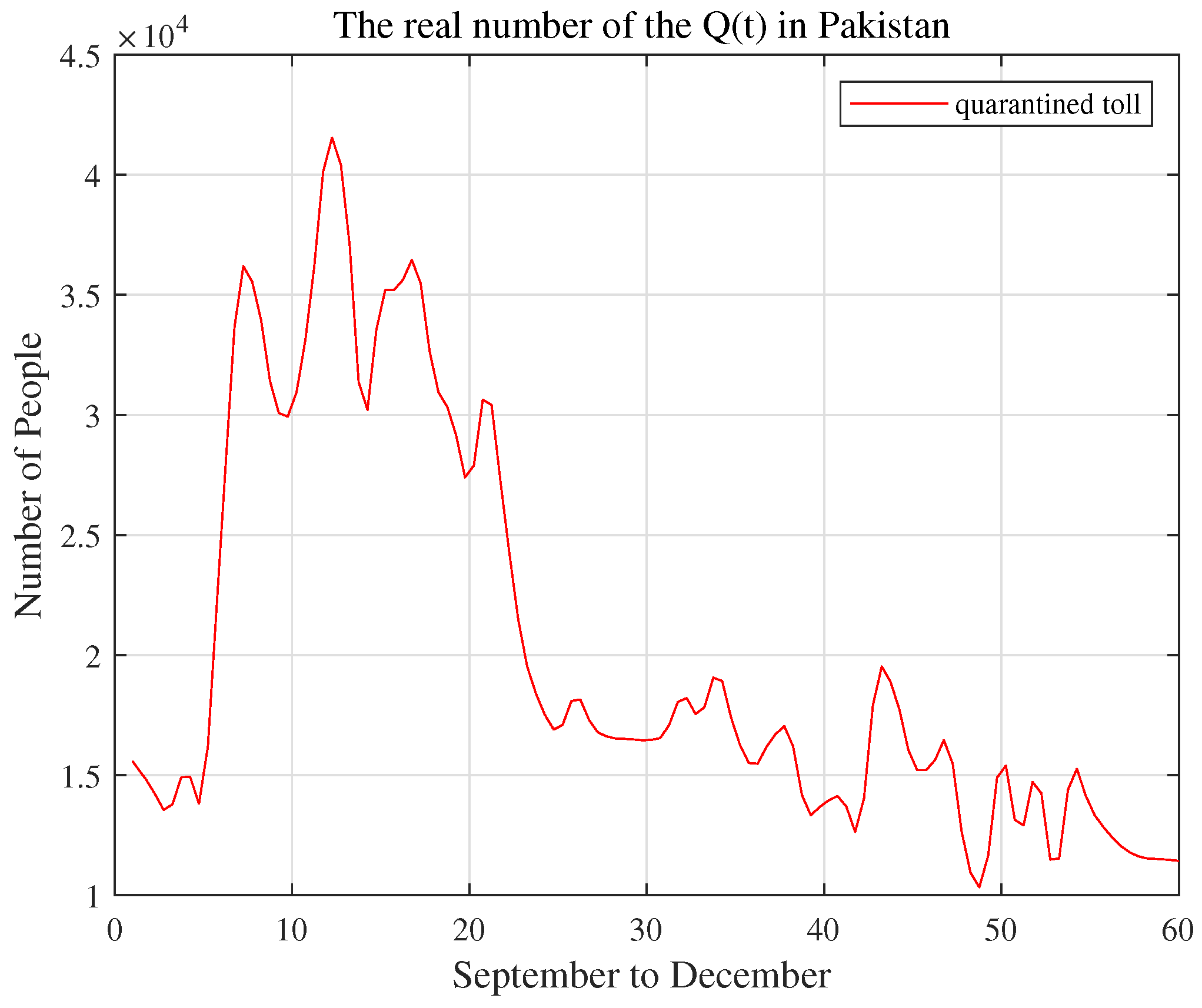
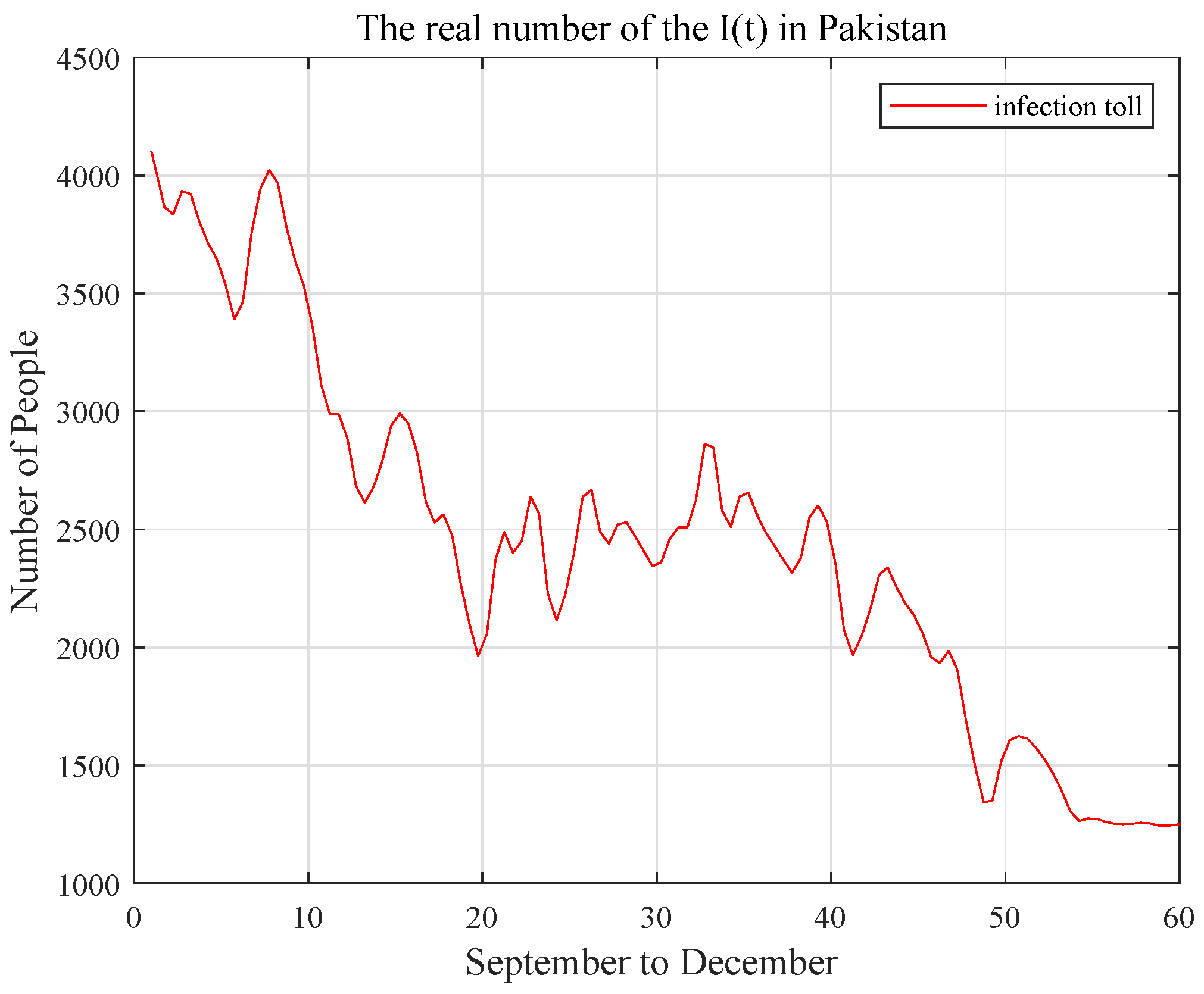
7. Examples and Numerical Simulations

In this section, we give the numerical simulation of system (3) by using the discrete equation with the same method as [10]. The equations are as follows:
S ( k + 1 ) = S ( k ) + [ Λ β S ( t ) I ( t ) N ( t ) μ 0 S ( t ) ] t η S ( t ) I ( t ) N ( t ) t ξ k η 2 2 S ( t ) I ( t ) N ( t ) t ( ξ k 2 1 ) , I ( k + 1 ) = I ( k ) + [ ( β S ( t ) I ( t ) N ( γ 1 + μ 1 + μ 0 ) I ( t ) + σ Q ( t ) ] t + η S ( t ) I ( t ) N ( t ) t ξ k + η 2 2 S ( t ) I ( t ) N ( t ) t ( ξ k 2 1 ) , Q ( k + 1 ) = Q ( k ) + [ γ 1 I ( t ) ( μ 0 + μ + σ ) Q ( t ) ] t ,
where the time increment t > 0 , and ξ k is a the Gaussian random variable ( k = 0 , 1 , 2 , n ) .
Example 1. 
Here, in system (3), we use the environmental noise parameter as η = 0.1 . In addition, following the biological feasibility result, the values of the parameters are as shown in Table 3.
In addition, we can choose the following real data S ( 0 ) = 355,250 , I ( 0 ) = 1453 , Q ( 0 ) = 51,343 , in Pakistan on 7 October 2021 [19]. Then, R 0 * = 3.208 > 1 , where R 0 * is defined in Section 4. By the results of Theorem 4, we can find that system (3) will persist for a long time by a distribution μ ( · ) . The numerical simulations (Figure 1) confirm this.
Example 2. 
Here, in system (3), we use the environmental noise parameter η = 0.1 . In addition, following the biological feasibility result, the values of the parameters are as shown in Table 4.
In addition, we can choose the following real data S ( 0 ) = 355,250 , I ( 0 ) = 1453 , Q ( 0 ) = 51,343 , in Pakistan on 7 October 2021 [19]. Then, R 0 * = 0.0769 < 1 , where R 0 * is defined in Section 4. We can find that system (3) will be extinct in a long time. The numerical simulations (Figure 2) confirm this.
In fact, using the statistical data of Pakistan for September to December 2021, it can be seen from the figure (Figure 3, Figure 4 and Figure 5) that the control of the isolation number will affect the disturbance of the infection rate and control the increase in the infection number. At the same time, when the infection rate is disturbed by other factors, such as vaccine injection, the number of deaths decreases with the decrease in the number of infections. This is basically consistent with the research results of system (3) in this paper.

8. Discussion

So far, the COVID-19 coronavirus disease is still one of the most serious diseases in the world. Until today, there is no appropriate treatment. At the same time, due to the strong transmission of the virus, with the existence of many uncertain factors (human activities, animal activities, express delivery, etc.), it also contains a lot of randomness. With the help of stochastic theory, we developed a model for the new 2019 coronavirus disease, and considered studying the transmission characteristics of the disease and understanding its transmission dynamics in the change in population and environment. The important role of isolation measures in controlling transmission is introduced. By disturbing the infection coefficient, the existence and positivity of Lyapunov function theory are studied. In this paper, in order to further discuss the extinction and stable distribution, we gave a new random infectious disease system under infection rate environmental noise. We give the existence and uniqueness of the solution of the system and discuss the ergodic stationary distribution and the extinction conditions of the system. The probability density function of the stochastic system is studied. Some digital simulations are used to demonstrate the probability density function and the extinction of system (3). Through numerical simulation, we analyzed the above results and drew a conclusion with the support of graphics. This work shows that random analysis is a better method used to study the dynamics of infectious diseases, especially the new 2019 coronavirus disease.
We know that the control of infectious diseases needs to consider a variety of random disturbance factors, and we will consider system (3) in more general random phenomena and their persistence and extinction properties in our future research.

Author Contributions

Writing—original draft preparation, J.S.; writing—review and editing, J.S. and M.G.; funding acquisition, J.S. and D.J. All authors have read and agreed to the published version of this manuscript.

Funding

The authors were supported by Shandong Provincial Natural Science Foundation (No. ZR2021MA052) and the National Natural Science Foundation of China (No. 11601520).

Institutional Review Board Statement

Not applicable.

Informed Consent Statement

Not applicable.

Data Availability Statement

Not applicable.

Conflicts of Interest

The authors declare no conflict of interest.

References

  1. Lai, C.C.; Shih, T.P.; Ko, W.C.; Tang, H.J.; Hsueh, P.R. Severe acute respiratory syndrome coronavirus 2 (SARS-CoV-2) and corona virus disease-2019 (COVID-19): The epidemic and the challenges. Int. J. Antimicrob. Agents 2020, 53, 105924. [Google Scholar] [CrossRef] [PubMed]
  2. Wu, Z.; Mcgoogan, J.M. Characteristics of and important lessons from the coronavirus disease 2019 (COVID-19) outbreak in china: Summary of a report of 72 314 cases from the chinese center for disease control and prevention. JAMA 2020, 323, 1239–1242. [Google Scholar] [CrossRef] [PubMed]
  3. Mao, X. Stochastic Differential Equations and Applications; Horwood: Chichester, UK, 1997. [Google Scholar]
  4. Has’miniskii, R. Stochastic Stability of Differential Equations; Horwood: Chichester, UK, 1997. [Google Scholar]
  5. Mao, X.; Marion, G.; Renshaw, E. Environmental Brownian noise suppresses explosions in population dynamics. Stoch. Process. Appl. 2002, 97, 95–110. [Google Scholar] [CrossRef]
  6. Alzahrani, E.O.; Khan, M.A. Modeling the dynamics of hepatitis E with optimal control. Chaos Solit. Fract. 2018, 116, 287–301. [Google Scholar] [CrossRef]
  7. Wilder-Smith, A.; Freedman, D.O. Isolation, quarantine, social distancing and community containment: Pivotal role for old-style public health measures in the novel coronavirus (2019-nCoV) outbreak. J. Travel Med. 2020, 27, taaa020. [Google Scholar] [CrossRef] [PubMed]
  8. Han, B.; Zhou, B.; Jiang, D.; Hayat, T.; Alsaedi, A. Stationary solution, extinction and density function for a high-dimensional stochastic SEI epidemic model with general distributed delay. Appl. Math. Comput. 2021, 405, 126236. [Google Scholar] [CrossRef]
  9. Thomas, C.G. Introduction to Stochastic Differential Equations; Dekker: New York, NY, USA, 1988. [Google Scholar]
  10. Gao, M.M.; Jiang, D.; Hayat, T.; Alsaedi, A. Threshold behavior of a stochastic Lotka-Volterra food chain chemostat model with jumps. Phys. A 2019, 523, 191–203. [Google Scholar] [CrossRef]
  11. Siqueira, J.D.; Goes, L.R.; Alves, B.M.; da Silva, A.C.P.; de Carvalho, P.S.; Cicala, C.; Arthos, J.; Viola, J.P.; Soares, M.A. Distinguishing SARS-CoV-2 bonafide re-infection from pre-existing minor variant reactivation, Infection. Genet. Evol. 2021, 90, 104772. [Google Scholar] [CrossRef] [PubMed]
  12. Lipster, R. A strong law of large numbers for local martingales. Stochastics 1980, 3, 217–218. [Google Scholar]
  13. Griffin, B.D.; Chan, M.; Tailor, N.; Mendoza, E.J.; Leung, A.; Warner, B.M.; Duggan, A.T.; Moffat, E.; He, S.; Garnett, L.; et al. SARS-CoV-2 infection and transmission in the North American deer mouse. Nat. Commun. 2021, 12, 3612. [Google Scholar] [CrossRef]
  14. Khan, M.A.; Abdon, A. Modeling the dynamics of novel coronavirus (2019-nCoV) with fractional derivative. Alex. Eng. J. 2020, 59, 2379–2389. [Google Scholar] [CrossRef]
  15. Abdon, A. Modelling the spread of COVID-19 with new fractal-fractional operators: Can the lockdown save mankind before vaccination. Chaos Solitons Fractals 2020, 136, 109860. [Google Scholar]
  16. Zhou, B.; Zhang, X.; Jiang, D. Dynamics and density function analysis of a stochastic SVI epidemic model with half saturated incidence rate. Chaos Solitons Fractals 2020, 137, 109865. [Google Scholar] [CrossRef]
  17. Chen, Y.; Cheng, J.; Jiang, Y.; Liu, K. A time delay dynamic system with external source for the local outbreak of 2019-nCoV. Appl. Anal. 2020, 12, 1–12. [Google Scholar] [CrossRef]
  18. Din, A.; Khan, A.; Baleanu, D. Stationary distribution and extinction of stochastic coronavirus (COVID-19) epidemic model. Chaos Solitons Fractals 2020, 139, 110036. [Google Scholar] [CrossRef] [PubMed]
  19. Available online: http://covid.gov.pk/ (accessed on 10 January 2022).
  20. Herwaarden, O.A.; Grasman, J. Stochastic epidemics: Major outbreaks and the duration of the endemic period. J. Math. Biol. 1995, 33, 581–601. [Google Scholar] [CrossRef] [PubMed]
  21. Roozen, H. An asymptotic solution to a two dimensional exit problem arising in population dynamics. SIAM J. Appl. Math. 1989, 49, 1973. [Google Scholar] [CrossRef] [Green Version]
  22. Hethcote, H.W. Qualitative analyses of communicable disease models. Math. Biosci. 1976, 28, 335–356. [Google Scholar] [CrossRef]
Figure 1. The red lines describe the solution of system (3) and the green lines stand for the solution of the corresponding system (2). The right pictures are the histogram of the density function for S , I , and Q populations.
Fractalfract 06 00245 g001
Figure 2. The red lines discribe the solution of system (3) and the green lines stand for the solution of the corresponding system (2). The right pictures are the histogram of the density function for S , I , and Q populations.
Fractalfract 06 00245 g002
Figure 3. The number of the daily statistics of quarantined people in Pakistan from September to December 2021.
Fractalfract 06 00245 g003
Figure 4. The red curve represents the daily statistics number of infections in Pakistan from September to December 2021.
Fractalfract 06 00245 g004
Figure 5. The blue curve represents the daily statistics death toll in Pakistan from September to December 2021.
Fractalfract 06 00245 g005
Table 1. The definitions of the parameters.
ParameterDefinitions
S ( t ) The susceptible class
I ( t ) Infected people
C ( t ) Carriers (dead corpse)
R ( t ) Recovered persons
D ( t ) Total number of deaths
μ Rate of natural death recruitment rate into S ( t )
θ Probability of an S ( t ) class to join C ( t ) class
σ Death rate induced by COVID-19
β Recovery rate of C ( t ) class
δ Force of infection of class S ( t )
τ Recovery rate of I ( t ) class
π Rate at which an C ( t ) class is recovered
η Rate at which treated persons become C ( t ) class
Table 2. The definitions of the parameters.
ParameterDefinitions
S ( t ) The susceptible class
I ( t ) Infected people
Q ( t ) Quarantined people
NTotal population
Λ Capita constant fecundity rate
β Infection rate
μ 0 Infected natural mortality rate
μ 1 Quarantined natural mortality rate
μ Disease-related mortality rate
γ 1 The constant rate of quarantining infected
σ The quarantined rate from infected people
B i ( t ) , i = 1 , 2 , 3 Brownian motion
η i , i = 1 , 2 , 3 The intensity of B i ( t )
Table 3. Parameters value.
NotationValueReferences
Λ 0.028[18]
β 0.2Estimated
μ 0 0.011[18]
μ 1 0.2Estimated
γ 0.06[18]
σ 0.3Estimated
μ 0.5[18]
Table 4. Parameters value.
NotationValueReferences
Λ 0.5[15]
β 0.6Estimated
μ 0 0.2[15]
μ 1 0.2Estimated
γ 0.3[15]
σ 0.1Estimated
μ 0.2[15]
Publisher’s Note: MDPI stays neutral with regard to jurisdictional claims in published maps and institutional affiliations.

