A Slow Single-Species Model with Non-Symmetric Variation of the Coefficients

Abstract

A single-species population model exhibiting a symmetric slow variation for the carrying capacity and intrinsic growth rate is evaluated explicitly. However, it is unrealistic to eliminate the possibility of a clear separation in the evolution of the biotic environmental elements; thus, this paper considers the situation where these elements have a hierarchical variation on the time scales. Accordingly, two particular situations are recognized, which are the carrying capacity varies faster than the growth rate and vice versa. Applying the multi-time scaling technique in such a system provides a small parameter, which leads us to construct analytical approximate expressions for the population behavior, using the perturbation approach. Such approximations display very good agreement with the numerical simulations.

1. Introduction

Describing the evolution of the population using the logistic growth model has an extensive research history. Such a model has been incorporated in numerous fields of biological applications, such as modeling yeast cultures [1], describing the human population [2], investigating a population of microorganisms [3], modeling the growth of fish school populations [4] and many other applications, presented in [5,6].

Considering the logistic model with constant environmental coefficients, the expression of the population behavior is well known in the literature—see, for example, the works of Banks [5] and Broun [6]. However, it is unrealistic to ignore the variation of the biotic environment which arises from the evolution of the ecosystem. Accordingly, Mayer and Ausubel [7] investigated the behavior of the human population utilizing the logistic model with a constant intrinsic growth rate, gradually increasing the carrying capacity. Their analysis provided the numerical solution for the population and shows very good agreement with experimental data of England and Japan populations. Similarly, Al-Moqbali et al. [8] investigated the stability along with obtaining the numerical solution of the prey–predator model with assuming a variable carrying capacity and fixed growth rate.

Assuming time-varying coefficients, the exact solution of the logistic model is no longer available, except in very special cases, so the numerical techniques must be adopted. However, although such a method provides expressions of the population behavior, it shows limited information for the evolution of the population in view of the influence of the environmental coefficients. In order to have a better understanding, an analytical approximate expression of the population evolution may be obtained via applying a multi-time scaling technique. Such a technique is well established in the literature for various fields—see, for example, [9,10,11,12]. Thus, Shepherd et al. [13] successfully applied the multi-time scaling technique to obtain the analytical expression of the logistic model, assuming a slow variation of the carrying capacity and a stationary growth rate. Their calculations were compared well with the exact solution. For the general case that the carrying capacity and growth rate both vary with time, Grozdanovski et al. [14] and Shepherd et al. [15] developed the methodology of applying the multi-time scaling method and obtained the analytical approximation for the population. They validated their result through comparing with the numerical solution under which was shown a very good accuracy with the analytical one. Following the calculation of [14], Idlango et al. [16,17,18] investigated the logistic model with harvesting, displaying the Allee effect and saturating harvesting. Their analysis shows the analytical expression for the population, in explicit and implicit forms, in the situation of subcritical and supercritical harvesting. These findings were compared with the numerical solution and showed favorable accuracy. Recently, Alsharidi et al. [19] investigated the anaerobic digestion model and obtained the expression by applying a parallel technique of those in [16,17,18].

Therefore, we aim in this paper to investigate the slow logistic model with asymmetric variation between the carrying capacity and the growth rate. This will allow the possibility of a clear separation in evolution of the environmental coefficients. We consider the multi-time scaling technique together with the perturbation approach to construct the analytical approximate expression of the population behavior. In addition, since the exact solution for our assumption is not available in the literature, we consider the numerical simulation using a fourth-order Runge–Kutta technique; we compare with the analytical approximation and find that the accuracy between the two methods is very good indeed.

2. Analytical Analysis

The non-autonomous single species population model may be written in the form,

$$\begin{array}{c}\hfill \frac{d\widehat{P}}{dT}=R\left(T\right)\widehat{P}\left(T\right)\left(1-\frac{\widehat{P}\left(T\right)}{K\left(T\right)}\right),\widehat{P}(T=0)={\widehat{P}}_0,\end{array}$$

(1)

where $\widehat{P}\left(T\right),R\left(T\right)$ and $K\left(T\right)$ represent the population density, growth rate and carrying capacity, respectively; all of them depend on the variable T, while ${\widehat{P}}_0$ is the initial population when $T=0$. Note that an explicit solution of (1) may be written as

$$\begin{array}{c}\hfill \widehat{P}\left(T\right)={\widehat{P}}_0{e}^{{\int }_0^{T}R\left(\zeta \right)d\zeta }{\left(1+{\widehat{P}}_0{\int }_0^T\left(\frac{R\left(\zeta \right)}{K\left(\zeta \right)}{e}^{{\int }_0^{\zeta }R\left(\eta \right)d\eta }\right)d\zeta \right)}^{-1},\end{array}$$

(2)

but due to the integral terms in (2), a full explicit solution to the population is only available for very special choices of $R\left(T\right)$ and $K\left(T\right)$ functions. Otherwise, a numerical technique must be employed.

Before constructing our analysis, we first non-dimensionalize the non-autonomous logistic model (1) by assuming $R\left(T\right)$ and $K\left(T\right)$ varying on the time scales $T_R$ and $T_K$, respectively. So, the functions $R\left(T\right)$ and $K\left(T\right)$ may be expressed in dimensionless form as follows

$$\begin{array}{c}\hfill R\left(T\right)=R_{0}r(T/T_R)\mathrm{and}K\left(T\right)=K_{0}k(T/T_K),\end{array}$$

(3)

where r and k are the dimensionless growth rate and carrying capacity, respectively, while $R_0$ and $K_0$ are the characteristic constants. Note that assuming constant environments, i.e., R and/or K are constant, which means that $R=R_0$ (and hence $r\equiv 1$) and/or $K=K_0$ (and hence $k\equiv 1$).

Regarding the dimensionless population $\widehat{P}\left(T\right)$, we introduce the dimensionless time by $t=R_{0}T$ and the dimensionless population by $\widehat{p}=\widehat{P}/K_0$. Thus, in a view of the above scalings, the dimensionless logistic model (1) can be expressed as

$$\begin{array}{c}\hfill \frac{d\widehat{p}}{dt}=r(t{R}_0^{-1}/T_R)\widehat{p}\left(t\right)\left(1-\frac{\widehat{p}\left(t\right)}{k(t{R}_0^{-1}/T_K)}\right),\widehat{p}(t=0)=\mu ,\end{array}$$

(4)

where $\mu$ is the dimensionless initial population corresponding to ${\widehat{P}}_0$.

At this stage, $R\left(T\right)$ and $K\left(T\right)$ are assumed to be varying on hierarchical time scales. So, there are two situations that are identified, which are $K\left(T\right)>R\left(T\right)$ and $R\left(T\right)>K\left(T\right)$. In what follows, we consider analyzing the situation where $K\left(T\right)>R\left(T\right)$, and we exhibit the solution of the population evolution when $R\left(T\right)>K\left(T\right)$ in the Discussion section.

Note that, from (4), when the time scales $T_R>T_K$ and both of them are large relative to $R_0^{-1}$, the variation of $r(t{R}_0^{-1}/T_R)$ is smaller than the small $k(t{R}_0^{-1}/T_K)$. Accordingly, the hierarchical relationship in variation between the coefficients might be established based on one small parameter as follows:

$$\begin{array}{c}\hfill \sqrt{ϵ}=\frac{R_0^{-1}}{T_K}\mathrm{and}ϵ=\frac{R_0^{-1}}{T_R},\end{array}$$

(5)

where $ϵ\ll 1$.

Applying (5) into (4) yields to the general dimensionless population model as

$$\begin{array}{c}\hfill \frac{d\widehat{p}}{dt}=r\left(ϵt\right)\widehat{p}(t,ϵ)\left(1-\frac{\widehat{p}(t,ϵ)}{k\left(\sqrt{ϵ}t\right)}\right),\widehat{p}(0,ϵ)=\mu .\end{array}$$

(6)

3. Multi-Time Scaling

Since the model (6) involves three time scales, which are the ordinary time variable t and the two slow time variables, $\sqrt{ϵ}t$ and $ϵt$, we adopt the multi-time scaling method by presenting the generalized ordinary time variable, $t_o$, and the two slow time variables, $t_k$ and $t_r$, as

$$\begin{array}{c}\hfill t_o=\frac{1}{\sqrt{ϵ}}w\left(t_k\right),t_k=\frac{1}{\sqrt{ϵ}}x\left(t_r\right)\mathrm{and}{t}_r=ϵt,\end{array}$$

(7)

where the subscripts k and r refer to the time scale for the carrying capacity and growth rate, respectively. Note that $w\left(t_k\right)$ and $x\left(t_r\right)$ are expected to be positive, continuous and differentiable functions on $t_k>0$ and $t_r>0$, with $w\left(0\right)=0$ and $x\left(0\right)=0$, respectively.

With respect to $t_r=ϵt$, the derivative of those in (7) are given by

$$\begin{array}{c}\hfill d{t}_o=w^{\prime }\left(t_k\right)x^{\prime }\left(t_r\right)dt,d{t}_k=\sqrt{ϵ}{x}^{\prime }\left(t_r\right)dt\mathrm{and}d{t}_r=ϵdt,\end{array}$$

(8)

and we point out, from (8), that the relationship between $t_o$ and t as well as $t_k$ and $\sqrt{ϵ}t$ are governed by the functions $w^{\prime }\left(t_k\right)$ and $x^{\prime }\left(t_r\right)$. Accordingly, we assume $w^{\prime }\left(t_k\right)>0$ and $x^{\prime }\left(t_r\right)>0$ to ensure that such relationships are monotonic. In a view of the above, we express the population solution $\widehat{p}(t,ϵ)$ as a function $p(t_o,t_k,t_r,ϵ)$ of these variables. With the application of the chain rule, the differential Equation (6) is translated to multi-timing scaled logistic equation as

$$\begin{array}{c}\hfill w^{\prime }\left(t_k\right)x^{\prime }\left(t_r\right)D_{o}p+\sqrt{ϵ}{x}^{\prime }\left(t_r\right)D_{k}p+ϵD_{r}p=r\left(t_r\right)p\left(1-\frac{p}{k\left(t_k\right)}\right),\end{array}$$

(9)

where $D_o,D_k$ and $D_r$ represent the partial derivatives of $t_o,t_k$ and $t_r$, respectively. Therefore, the multi-time scaling is successfully applied to the differential Equation (6) and such an equation becomes a partial differential equation for the unknown $p(t_o,t_k,t_r,ϵ)$. Since the parameter $ϵ$, which governs the order of the coefficients variation, appears explicitly in (9) rather than implicitly in (6), the perturbation method based on a small $ϵ$ is employed to explicitly obtain the analytical approximate expression for the population of (6) that is valid for all $t>0$.

4. Perturbation Analysis

In what follows, we apply the perturbation approach based on a small $ϵ$ to the partial differential Equation (9). This yields to express $p(t_o,t_k,t_r,ϵ)$ in power of $ϵ$ as

$$\begin{array}{c}\hfill p(t_o,t_k,t_r,ϵ)=p_0(t_o,t_k,t_r)+\sqrt{ϵ}{p}_1(t_o,t_k,t_r)+ϵp_2(t_o,t_k,t_r)+\dots ,\end{array}$$

(10)

then substituting (10) into (9) and equating the coefficients of like power of $ϵ$ give the leading and higher orders terms as

$$\begin{array}{cc}& w^{\prime }\left(t_k\right)x^{\prime }\left(t_r\right)D_o{p}_0=r\left(t_r\right)p_0\left(1-\frac{p_0}{k\left(t_k\right)}\right),\end{array}$$

(11)

$$\begin{array}{cc}& w^{\prime }\left(t_k\right)x^{\prime }\left(t_r\right)D_o{p}_1-r\left(t_r\right)\left(1-\frac{2p_0}{k\left(t_k\right)}\right)p_1=-x^{\prime }\left(t_r\right)D_k{p}_0,\end{array}$$

(12)

$$\begin{array}{cc}& w^{\prime }\left(t_k\right)x^{\prime }\left(t_r\right)D_o{p}_2-r\left(t_r\right)\left(1-\frac{2p_0}{k\left(t_k\right)}\right)p_2=-D_r{p}_0-x^{\prime }\left(t_r\right)D_k{p}_1-\frac{r\left(t_r\right)}{k\left(t_k\right)}{p}_1^2.\end{array}$$

(13)

Solving (11) for $p_0(t_o,t_k,t_r)$ gives

$$\begin{array}{c}\hfill p_0(t_o,t_k,t_r)=\frac{k\left(t_k\right)}{1+A(t_k,t_r)k\left(t_k\right)e^{-\beta \left(t_k\right)\theta \left(t_r\right)t_0}},\end{array}$$

(14)

where $\beta \left(t_k\right)$ and $\theta \left(t_r\right)$ are given by

$$\begin{array}{c}\hfill \beta \left(t_k\right)=\frac{1}{w^{\prime }\left(t_k\right)}>0\theta \left(t_r\right)=\frac{r\left(t_r\right)}{x^{\prime }\left(t_r\right)}>0,\end{array}$$

(15)

and $A(t_k,t_r)$ is an arbitrary function of $t_k$ and $t_r$ to be determined later.

In a similar manner, solving (12), on applying (14), we obtain the particular solution for $p_1(t_o,t_k,t_r)$ as

$$\begin{array}{ccc}{p}_1(t_o,t_k,t_r)& =& \frac{1}{{(1+A(t_k,t_r)k\left(t_k\right)e^{-\beta \left(t_k\right)\theta \left(t_r\right)t_o})}^2}\left[k^2\left(t_k\right)e^{-\beta \left(t_k\right)\theta \left(t_r\right)t_o}\right(A^{\prime }(t_k,t_r)t_o-\\ & & \frac{A(t_k,t_r){\beta }^{\prime }\left(t_k\right)\theta \left(t_r\right)t_o^2}{2})-\frac{k^{\prime }\left(t_k\right)}{\beta \left(t_k\right)\theta \left(t_r\right)}],\end{array}$$

(16)

where the primes in $A^{\prime }(t_k,t_r),{\beta }^{\prime }\left(t_k\right)$ and $k^{\prime }\left(t_k\right)$ represent the derivative with respect to $t_k$.

It is important to note that as $t_o\to \infty$, $p_0(t_o,t_k,t_r)$, given in (14), reaches the carrying capacity limit $k\left(t_k\right)$, and in (16), $p_1(t_o,t_k,t_r)$ reaches $-\frac{k^{\prime }\left(t_k\right)}{\beta \left(t_k\right)\theta \left(t_r\right)}$. However, the rate of convergence of $p_0(t_o,t_k,t_r)$ is exponential, while that of $p_1(t_o,t_k,t_r)$ is not. This asymmetry arises due to the presence of a quadratic polynomial function of $t_o$ in (16). Consequently, we argue that the rate of convergence of $p_1(t_o,t_k,t_r)$ must be aligned to reach its limit at the same time as that of $p_0(t_o,t_k,t_r)$. To achieve this, we apply parallel justifications to those of [16] and separately set the coefficients of $t_o$ and $t_o^2$ in (16) to zero. This yields

$$\begin{array}{c}\hfill A^{\prime }(t_k,t_r)=0,A(t_k,t_r){\beta }^{\prime }\left(t_k\right)\theta \left(t_r\right)=0.\end{array}$$

(17)

Thus, the first of (17) leads to concluding that $A(t_k,t_r)=\alpha \left(t_r\right)$, while in the second, we only have to select ${\beta }^{\prime }\left(t_k\right)=0$ to satisfy the equation, and hence $\beta \left(t_k\right)$ is constant. In particular and for simplicity, we may choose $\beta \left(t_k\right)=1$ and, accordingly, the first of (15) becomes $w^{\prime }\left(t_k\right)=1$.

Considering the above observations and results, (16) is reduced to

$$\begin{array}{c}\hfill p_1(t_o,t_k,t_r)=-\frac{k^{\prime }\left(t_k\right)}{\theta \left(t_r\right){(1+\alpha \left(t_r\right)k\left(t_k\right)e^{-\theta \left(t_r\right)t_o})}^2}.\end{array}$$

(18)

Solving the second correction term, given in (13), we obtain the solution of $p_2(t_o,t_k,t_r)$ as follows

$$\begin{array}{ccc}{p}_2(t_o,t_k,t_r)& =& \frac{{\theta }^{-2}\left(t_r\right)k^{-1}\left(t_k\right)}{{(1+\alpha \left(t_r\right)k\left(t_k\right)e^{-\theta \left(t_r\right)t_o})}^2}[\frac{{\theta }^2\left(t_r\right)k^3\left(t_k\right)e^{-\theta \left(t_r\right)t_o}}{x^{\prime }\left(t_r\right)}\left({\alpha }^{\prime }\left(t_r\right)t_o-\frac{\alpha \left(t_r\right){\theta }^{\prime }\left(t_r\right)t_o^2}{2}\right)+\\ & & k\left(t_k\right)k^{″}\left(t_k\right)-k^{\prime 2}\left(t_k\right)+\frac{{\alpha }^2\left(t_r\right)k^{\prime 2}\left(t_k\right)k^2\left(t_k\right)e^{-2\theta \left(t_r\right)t_o}}{1+\alpha \left(t_r\right)k\left(t_k\right)e^{-\theta \left(t_r\right)t_o}}],\end{array}$$

(19)

where the primes in ${\alpha }^{\prime }\left(t_r\right)$ and ${\theta }^{\prime }\left(t_r\right)$ denote the derivative with respect to $t_r$, while in $k^{\prime }\left(t_k\right)$, they represent the derivative with respect to $t_k$. Applying analogous observations to that in (16), we conclude that ${\alpha }^{\prime }\left(t_r\right)=0$, and hence $\alpha \left(t_r\right)=c$, where c is an arbitrary constant to be found using the initial condition, given in (6). Furthermore, ${\theta }^{\prime }\left(t_r\right)=0$, so $\theta \left(t_r\right)$ is constant, and for simplicity we choose $\theta \left(t_r\right)=1$. Consequently, we conclude form the second of (15) that $x^{\prime }\left(t_r\right)=r\left(t_r\right)$ and accordingly, the first and the second of (8) become

$$\begin{array}{c}\hfill t_o=\frac{1}{ϵ}{\int }_0^{t_r}r\left(s\right)ds,t_k=\frac{1}{\sqrt{ϵ}}{\int }_0^{t_r}r\left(s\right)ds,\end{array}$$

(20)

defining the variables $t_o$ and $t_k$ completely in terms of the growth rate function.

With respect to the observation above, (19) is reduced to

$$\begin{array}{cc}\hfill & p_2(t_o,t_k,t_r)=\frac{k^{-1}\left(t_k\right)}{{(1+ck\left(t_k\right)e^{-t_o})}^2}\left(k\left(t_k\right)k^{″}\left(t_k\right)-k^{\prime 2}\left(t_k\right)+\frac{c^2{k}^{\prime 2}\left(t_k\right)k^2\left(t_k\right)e^{-2t_o}}{1+ck\left(t_k\right)e^{-t_o}}\right).\end{array}$$

(21)

To recapitulate, applying (14), (18) and (21) into the expansion (10) yields, on considering the results arising from the observations,

$$\begin{array}{ccc}\hfill p(t_o,t_k,t_r,ϵ)& =& \frac{k\left(t_k\right)}{1+ck\left(t_k\right)e^{-t_o}}-\frac{\sqrt{ϵ}{k}^{\prime }\left(t_k\right)}{{(1+ck\left(t_k\right)e^{-t_o})}^2}+\frac{ϵk^{-1}\left(t_k\right)}{{(1+ck\left(t_k\right)e^{-t_o})}^2}\times \hfill \\ & & \left[k\left(t_k\right)k^{″}\left(t_k\right)-k^{\prime 2}\left(t_k\right)+\frac{c^2{k}^{\prime 2}\left(t_k\right)k^2\left(t_k\right)e^{-2t_o}}{1+ck\left(t_k\right)e^{-t_o}}\right]+\dots ,\hfill \end{array}$$

(22)

where the prime denotes to the derivative with respect to $t_k$. Since our expansion, given in (10), is built with $\mathcal{O}\left(1\right),\mathcal{O}\left(\sqrt{ϵ}\right)$ and $\mathcal{O}\left(ϵ\right)$, we assume that c in (22) follows a similar manner and take the form $c=c_0+c_1\sqrt{ϵ}+c_2ϵ$. Thus, with c expansion, (22) yields, on expansion of the like power of $ϵ$,

$$\begin{array}{cc}& p(t_o,t_k,t_r,ϵ)=\frac{k\left(t_k\right)}{F(t_o,t_k)}-\frac{\sqrt{ϵ}}{F^2(t_o,t_k)}\left(c_1{k}^2\left(t_k\right)e^{-t}+k^{\prime }\left(t_k\right)\right)+\frac{ϵ}{F^2(t_o,t_k)}[\frac{k\left(t_k\right)k^{″}\left(t_k\right)-k^{\prime 2}\left(t_k\right)}{k\left(t_k\right)}-\\ & c_2{k}^2\left(t_k\right)e^{-t_o}+\frac{k\left(t_k\right)e^{-2t_o}}{F(t_o,t_k)}\left(c_0^2{k}^{\prime 2}\left(t_k\right)+c_1^2{k}^2\left(t_k\right)+2c_1{k}^{\prime }\left(t_k\right)e^{t_o}\right)]+\dots ,\end{array}$$

(23)

where the function $F(t_o,t_k)$ is given by

$$\begin{array}{c}\hfill F(t_o,t_k)=1+c_{0}k\left(t_k\right)e^{-t_o},\end{array}$$

(24)

and the constants $c_0,c_1$ and $c_2$ are given by substituting the initial condition (6) into (23) on equating the like power of $ϵ$ and then are solved. Thus, these take the form as

$$\begin{array}{c}\hfill c_0=\frac{1}{\mu }-\frac{1}{k\left(0\right)},c_1=-\frac{k^{\prime }\left(0\right)}{k^2\left(0\right)},c_2=\frac{k^{″}\left(0\right)}{(k^2\left(0\right)}+\frac{k^{\prime }2\left(0\right)(k\left(0\right)-3\mu )}{k^3\left(0\right)\mu }.\end{array}$$

(25)

5. Results and Discussion

In this paper, the analytical approximate expression for the population of the slow logistic model with the non-parallel variation of the coefficients is readily and explicitly obtained, and the expansion (23) represents the result. It should be noted that the perturbation expansion (10) is limited to the first three terms of the series, and this is due to the observation that the three-term solution provides a remarkable accuracy without swell of the expression. In the limit of $ϵ\to 0$ along with considering a constant coefficients, (23) reduces to an exact solution—see, for example, [5]. In addition, when $t\to \infty$, the population in (23) reaches

$$\begin{array}{c}\hfill k\left(t_k\right)-\sqrt{ϵ}{k}^{\prime }\left(t_k\right)+ϵ\left(\frac{k\left(t_k\right)k^{″}\left(t_k\right)-k^{\prime 2}\left(t_k\right)}{k\left(t_k\right)}\right)+\dots ,\end{array}$$

(26)

varying close to the carrying capacity, $k\left(t_k\right)$, where $t_k$ is given in the second of (20). Note that for the long term, the slope of the carrying capacity trajectory becomes zero, i.e., $k^{\prime }\left(t_k\right)=0$ (and hence $k^{″}\left(t_k\right)=0)$. Thus, the population $p(t_o,t_k,t_r,ϵ)$ will eventually reach $k\left(t_k\right)$.

The relationship between the variables $t_r,t_k$ and $t_o$ is described in (20), and when the growth rate is assumed constant, for example, $r\left(t_r\right)\equiv 1$, then $t_k\equiv \frac{1}{\sqrt{ϵ}}{t}_r$ and $t_o\equiv \frac{1}{ϵ}{t}_r$, where $t_r=ϵt$. Such a relationship is realistic in describing the population through a variation of a biotic environment.

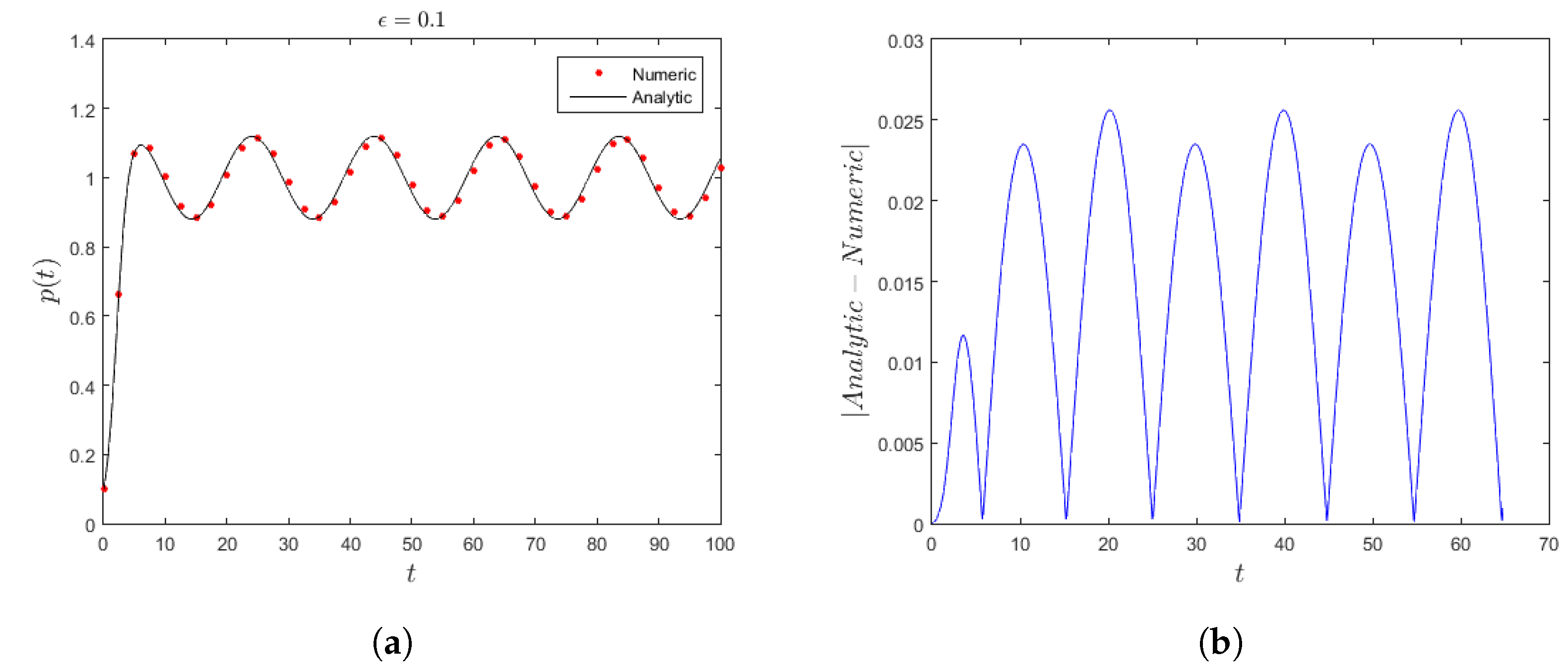
Since there is no exact solution for our assumption provided in the literature, we consider obtaining a numerical solution of our system, utilizing the fourth-order Runge–Kutta technique. Then, such a result is compared with the analytical approximation to validate the accuracy. To do that, we first consider that the carrying capacity, $k\left(t_k\right)$ is a periodic function, while the growth rate, $r\left(t_r\right)$, is an exponential decay function. These are given by

$$\begin{array}{c}\hfill k\left(t_k\right)=1+0.12sin\left(t_k\right),r\left(t_r\right)=1+0.12e^{-t_r}.\end{array}$$

(27)

Accordingly, Figure 1a, generated from the analytical approximation (23) (solid curve) along with the numerical solution (dotted curve), displays the population evolution from $\mu =0.1$ for slowly varying $k\left(t_k\right)$ and $r\left(t_r\right)$ coefficients, given in (27). It can clearly be seen that the comparison between the two methods shows very good agreement for $ϵ=0.1$. In the same context, Figure 1b, obtained by measuring the absolute difference between the approximate and numerical solution as $t\to \infty$, displays that the maximum discrepancy is less than $2.6\%$, which is a favorable accuracy.

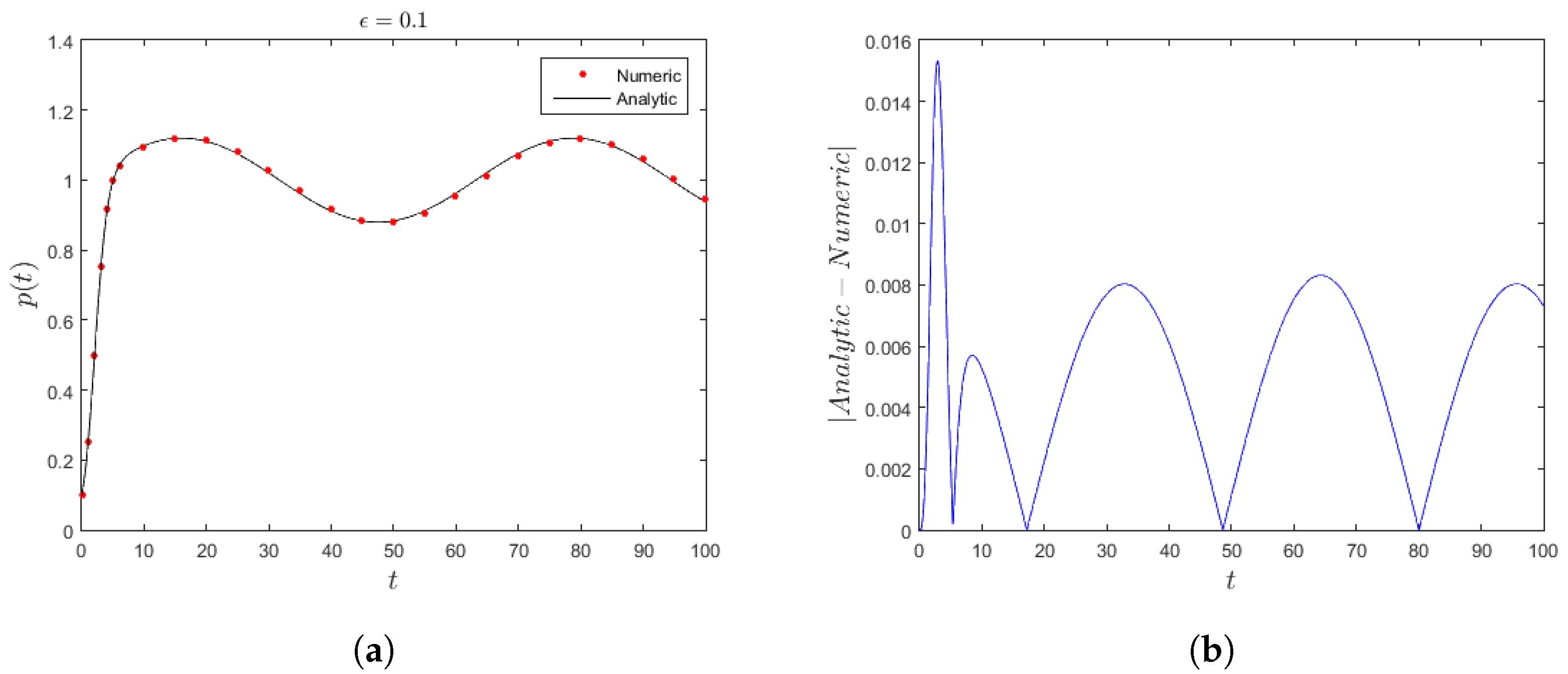
Note that we assume, earlier in this paper, that $K\left(T\right)>R\left(T\right)$. So, it is convenient to consider a solution for the population evolution when $R\left(T\right)>K\left(T\right)$. Consequently, applying analogous line of the above calculations, we reach the population expression as follows:

$$\begin{array}{cc}& p(t_o,t_k,t_r,ϵ)=\frac{k\left(t_k\right)}{H(t_o,t_k)}+\sqrt{ϵ}\left(\frac{k^2\left(t_k\right)k^{\prime }\left(0\right)e^{-t_o}}{H^2(t_o,t_k)k\left(0\right)r\left(0\right)\mu }-\frac{k^{\prime }\left(t_k\right)}{r\left(t_r\right)H(t_o,t_k)}\right)+\\ & ϵk\left(t_k\right)k^{\prime }\left(0\right)e^{-t_o}\left(\frac{k^2\left(t_k\right)k^{\prime }\left(0\right)e^{-t_o}}{H^3(t_o,t_k)k^2\left(0\right)r^2\left(0\right){\mu }^2}-\frac{k^{\prime }\left(t_k\right)}{r\left(t_r\right)H^2(t_o,t_k)k\left(0\right)r\left(0\right)\mu }\right)+\dots ,\end{array}$$

(28)

where $H(t_o,t_k),t_o,t_r$ and $t_k$ are given by

$$\begin{array}{c}\hfill H(t_o,t_k)=1+\left(\frac{1}{\mu }-\frac{1}{k\left(0\right)}\right)k\left(t_k\right)e^{-t_o},t_o=r\left(t_r\right)t,t_r=\sqrt{ϵ}t,t_k=ϵt,\end{array}$$

(29)

respectively.

Applying (27) in (28) together with considering the fourth-order Runge–Kutta technique for the numerical result generates Figure 2a, which displays the population evolution from $\mu =0.1$ to the equilibrium state where the coefficients very slowly. The accuracy between the two methods is very good for $ϵ=0.1$. In addition, Figure 2a shows that the variation of the carrying capacity is much slower than that in Figure 1a for the same period of time. This is due to changing the order of the coefficients’ variation. Moreover, for $t\to \infty$, the absolute difference between the approximate solution and the numerical simulation is less than $1.6\%$ as shown in Figure 2b.

6. Conclusions

The analytical approximation of the slow logistic population model with asymmetric variation coefficients was readily and explicitly obtained using the multi-time scaling technique. Such a result is adequate for a wide range of parameter values. In addition, the results of the numerical computations were obtained using the fourth-order Runge–Kutta technique and show very good agreement with the analytical one.