Article

Analytical Solutions of a Class of Fluids Models with the Caputo Fractional Derivative

Department of Mathematics, Cheikh Anta Diop University, Dakar Fann BP 5683, Senegal
Fractal Fract. 2022, 6(1), 35; https://doi.org/10.3390/fractalfract6010035
Submission received: 28 November 2021 / Revised: 5 January 2022 / Accepted: 6 January 2022 / Published: 11 January 2022

Abstract

:
This paper studies the analytical solutions of the fractional fluid models described by the Caputo derivative. We combine the Fourier sine and the Laplace transforms. We analyze the influence of the order of the Caputo derivative the Prandtl number, the Grashof numbers, and the Casson parameter on the dynamics of the fractional diffusion equation with reaction term and the fractional heat equation. In this paper, we notice that the order of the Caputo fractional derivative plays the retardation effect or the acceleration. The physical interpretations of the influence of the parameters of the model have been proposed. The graphical representations illustrate the main findings of the present paper. This paper contributes to answering the open problem of finding analytical solutions to the fluid models described by the fractional operators.

1. Introduction

Recently, fractional calculus has attracted much attention, and many papers have been published addressing the real applications of fractional calculus in real-world problems [1,2,3,4,5,6,7]. Many discussions have been had related to the utility of fractional calculus and where this field can be applied. Nowadays, many papers are addressing the utility of fractional calculus and the methods used to model the so-called fractional operators [8,9,10,11,12,13]. Note that, regarding the existing literature, fractional calculus can be applied in many fields such as modeling epidemic model [14], in sciences and engineering [15], in physics, and in others [16]. The existing fractional operators can be divided into two categories. The first is singular operators: the Caputo derivative and the Riemann–Liouville derivative [9,10]. These two derivatives are the most used in the literature. We also have the non-singular derivative as the Caputo–Fabrizio derivative and the Atangana–Baleanu derivative [11]. Many other derivatives in the literature exist such as the conformable derivative and the Hilfer derivative. Still, here we limited our citations to the most used derivatives in the literature of fractional calculus.
In the present paper, we model fluids using the Caputo derivative. Many papers deal with modeling fluid models with fractional operators. In [17], the authors propose the solutions for natural convection flow subject to arbitrary velocity and Newtonian heating. In [18], Kalid et al. propose a study on the unsteady MHD freeflow of a Casson fluid past an oscillating vertical plate with constant wall temperature and propose the method for obtaining a fluid model using Laplace transform. In [19], Khan et al. investigate using the Laplace transform of the Atangana–Baleanu derivative, the exact solutions of the constructive equations in the study of the second-grade fluids flow with combined gradients of mass concentration, and temperature distribution over a vertical flat plate. In [20], the authors propose the solutions of type of Casson fluid models. In [21], the authors use the Laplace transform of the Mittag–Leffler fractional operators in proposing the analytical solutions for the governing equations of the thermal diffusion process in terms of fractional differentiation. In [22], Sene proposes the solution of the second-grade fluid using integral balance methods. We mean that the double integral method and the heat balance the integral method. In [23], the authors also investigate getting the exact solutions of the constructive equations of the convective flow of a generalized Casson fluid. In [24], Abro and Atangana give a comparative presentation of convective fluid motion in a rotating cavity described by the non-singular fractal-fractional operators for differentiation. In [25], Ali et al. apply the derivative with the exponential kernel to MHD free convection flow of generalized Walters’-B fluid model. See also in the following investigations [24,26,27,28].
The modeling of the fluid model with Caputo derivative permits us to take into account the memory effect. However, finding the exact solutions is a problem. In the literature of fractional differential, there are many methods to get the solutions of the fractional differential equations. We can cite the homotopy analysis method and the numerical methods as the implicit scheme, explicit scheme, Adams–Basforth methods, and others. In this paper, we propose a technique for getting the solutions of a class of fluid models. The technique is the combination between the Laplace transform and Fourier transform. The method permits us to get the exact solutions of the fluid models; therefore, we do not need to utilize the integral balance methods and the numerical discretizations. The novelty will be the use of the Caputo derivative and its Laplace transform. We will provide the order of the Caputo derivative that has retardation and acceleration effects in the dynamics of the considered model. The influence of the Prandtl number, the Grashof numbers, and the Casson parameter will be analyzed and interpreted physically.
The paper is structured as follows. In Section 2, we recall the fractional operators as Caputo derivative, Riemann–Liouville integral, and the Riemann–Liouville derivative. In Section 3, we present the constructive equations of the fluid model; we will present the model using the Caputo derivative. The procedure to obtain the solutions with Fourier and the Laplace transform will be presented in Section 4. In Section 5, we discuss the findings of our paper. The final remarks and conclusion will be described in Section 6.

2. Fractional Calculus Operators

This section is devoted to recalling the fractional operators. We mean the Riemann–Liouville integral, the Caputo derivative, and the Riemann–Liouville integral. The other fractional operators, such as the fractional operators without singular kernels, will be referenced, and the readers can check the cited paper for these operators. In this paper, the Caputo derivative will be considered in our modeling due to its physical relationship with real-world problems. We have the following definitions that will be considered.
Definition 1.
The Riemann–Liouville integral [9,10] of a considered function h : [ 0 , + [ R can be represented as the following form
I α h ( t ) = 1 Γ ( α ) 0 t t s α 1 h ( s ) d s ,
where Γ ( ) represents the Gamma function and with order α satisfying the condition that α > 0 .
Definition 2.
We describe the Riemann–Liouville derivative [9,10] of the considered function h : [ 0 , + [ R , of order α as the form
D α h ( t ) = 1 Γ 1 α d d t 0 t h ( s ) t s α d s ,
where t > 0 , is the order of the operator that obeys the assumption that α 0 , 1 and Γ ( ) symbolize the Gamma Euler function.
In our modeling, we use the so-called Caputo derivative [9,10]. This derivative is the most used in the literature of fractional calculus. It is used because it considers the so-called memories effect, and the derivative of a constant function gives zero. It is well known that the fractional operators do not satisfy classical properties in derivations. We outline them in the following definitions.
Definition 3.
We represent the Caputo fractional operator with the considered function h : [ 0 , + [ R , of order α as the following representation
D α h ( t ) = 1 Γ 1 α 0 t d h ( s ) d s t s α d s ,
where t > 0 is the order of the operator that obeys the assumption that α 0 , 1 and Γ ( ) symbolizes the Gamma Euler function.
For the resolutions of the differential equations, including the fractional operators, their Laplace transform plays an important role. The role of the Laplace transform is, in general, to obtain analytical solutions. It is used in many methods such as the Homotopy analysis method, the homotopy perturbation method, and the domain decomposition method. The Laplace transform of the Caputo operator [9,10] can be represented as the following form
L D c α h ( t ) = s α L h ( t ) s α 1 h ( 0 ) ,
where the order α obeys the relationship α ( 0 , 1 ) .
For information related to the other new fractional operators as the conformable derivative [8] and the Caputo and Riemann–Liouville derivative, see paper [9,10]; for the derivative with Mittag–Leffler kernel, see the paper [11]; and for the Caputo–Fabrizio derivative, see paper [29]. For the above-cited derivative, it is also important to mention that their fractional integrals and Laplace transforms exist. The solution for the Cauchy problem can be obtained via the Laplace transforms.

3. Constructive Equations

In this section, we present the constructive equations subject of investigations. The novelty will be the consideration of the Caputo derivative in the modeling. We suppose the flow in x-direction, and we consider the y-axis to be normal to the plate. Let the initial time mean t = 0 ; we presume that the plate starts motion on its own plane with velocity considered constant U . Note that the temperature of the plate is considered to be T w at time t. As mentioned in the papers [23,30], the rheological equation for an incompressible Casson fluid can be represented as the following forms
π i j = 2 μ γ + p y 2 π e i j   when   π > π c ,
and
π i j = 2 μ γ + p y 2 π c e i j   when   π < π c .
In Equations (5) and (6), π = e i j e i j , μ denotes the dynamic viscosity, e i j represents ( i j ) th component of the deformation rate, p y symbolizes the yields stress, π c is the critical value of the number π , and μ γ denotes the plastic dynamic viscosity of the non-Newtonian flow. The governing equations, including the velocity and the temperature for free convection flow of the Casson fluid, can be represented using Caputo fractional derivative as the following form
ρ D α u = μ B 1 + 1 β 2 u x 2 + ρ g γ T T ,
and
ρ c p D t α T = k 2 T x 2 ,
with the initial and boundary conditions defined as the following forms
t < 0 : u = 0 , T = T x > 0 ,
t 0 : u = U , T = T w   at   x = 0 ,
u 0 , T T   as   x ,
where ρ is fluid density, c p is the specific heat capacity of fluid, k represents the thermal conductivity, μ B is the dynamic viscosity of fluids, β is the material parameter of Casson fluid, g represents the acceleration constant, and γ is the volumetric coefficient of thermal expansion. Let us simplify Equations (7) and (8) by using the so-called in literature the dimensionless variables given us the following forms
u = u U x = U ν x t = U 2 ν t ,
v = T T T w T , w = w ν U 2 , τ = τ ρ u 2 .
Using the above following variables changes for our system (7) and (8), we can represent the model (7) and (8) under consideration in our paper by the following forms
D τ α u = 2 u x 2 + 1 β 2 u x 2 + G r v ,
and
D τ α v = 1 P r 2 v x 2 ,
with the initial conditions given by
u ( x , 0 ) = 0 ,
v ( x , 0 ) = 0 ,
and the functions u and v have as boundary conditions the following relations
u ( 0 , τ ) = 1 ,
v ( 0 , τ ) = 1 .
Furthermore, we set the Prandtl number, the Grashof numbers, and the Casson parameter, respectively, as the forms
P r = μ c p k , G r = ν g γ T w T U 3 , β = μ B 2 π c p x .
This paper aims to propose the analytical solution of the fractional differential equation defined by the above Equations (14) and (15). Some investigations address the model presented in this paper. In these papers, they determined the analytical solutions using the Laplace transform, and after transformation, they will have to solve second-order differential equations and use the classical method to solve them. The difference with the existing investigation is that we combine the Laplace transform and the Fourier sine transforms to obtain the analytical solution. The method is valuable, and the implementation is not difficult. Another new aspect of this paper is the new initial conditions (18) and (19) and the use of the Caputo derivative in the investigation.

4. Solutions Procedures

There are many methods for determining the solutions for the fractional differential equations in the class of equations described in Equations (14) and (15). In this section, we describe the method to obtain the solutions with analytical techniques. We can cite the homotopy methods most used in fluid and nanofluid models; we mean the homotopy analysis and homotopy perturbation methods. The numerical methods can be seen, for example, in [31]. In the present investigation, we propose the exact solutions of our current model using the Laplace transform and the Fourier sine transformation. The combination between the Laplace transform and the Fourier sine transform is reported in the literature in the following investigations [28,32] and can also be found in many other papers. The advantage of this method in the present paper is it permits the obtaining of the linear fractional differential equations. The Laplace transform permits obtaining of the exact analytical solution by applying the inverse of the Laplace transform to the linear fractional differential equation obtained after the application of the Fourier sine transform. We can also observe that in the form of the solutions, there exists an improper integral, which is due to the formula of the inverse of the Fourier sine transform. The Laplace transform of the Caputo derivative will play an essential role in our investigations. The first step of the procedure will consist of applying sine transformation to the considered equations.

4.1. Temperature Distribution

Let us consider the heat equation represented in Equation (15), which is subject to the initial and boundary conditions in Equations (17) and (19). We have the following equation
D τ α v = 1 P r 2 v x 2 .
Note that using the classical formula of the Fourier sine transform, we have that F D α v ( x , τ ) = D α v ( q , τ ) and F 2 v x 2 = 2 q P r π v ( 0 , τ ) q 2 P r v ( q , τ ) , where F denotes the Fourrier sine transformation and q is the Fourrier sine variable [28]. We apply the Fourier sine transformation to this previous equation, and we obtain the following relationship
D c α v ( q , τ ) = 2 q P r π v ( 0 , τ ) q 2 P r v ( q , τ ) .
The second step will be to Laplace the Laplace transformation, including the Laplace transform to the Caputo derivative; after minor rearrangement, we get the following relationship
s α v ¯ ( q , s ) s α 1 v ( q , 0 ) + q 2 P r v ¯ ( q , s ) = 2 q P r π s , s α v ¯ ( q , s ) + q 2 P r v ¯ ( q , s ) = 2 q P r π s , v ¯ ( q , s ) = 2 q P r π s s α + q 2 P r , v ¯ ( q , s ) = 2 q π 1 s s α 1 s α + q 2 P r .
To obtain the solution of the heat equation with fractional order derivative according to the investigations in [28], we apply the inverse of the Laplace and obtain the following relation
v ( q , τ ) = 2 q π 1 E α q 2 P r τ α .
Following the procedure in [28], we should apply the inverse of the Fourier transform to Equation (24). Note that by using the formula of the inverse of the Fourier transform, an improper integral will appear and is due to the used formula, which is 2 π 0 + sin q x q v ( q , τ ) d q ; thus, we get the following solution
v ( x , τ ) = 2 π 0 + sin q x q 1 E α q 2 P r τ α d q , v ( x , τ ) = 2 π 0 + sin q x q d q 2 π 0 + sin q x q 1 E α q 2 P r τ α d q , v ( x , τ ) = 1 2 π 0 + sin q x q E α q 2 P r τ α d q .
Similar results in the integer-order version can be found in [28]. The transformation (23) is also vital in diffusion equations. It is used in physics to determine the so-called mean square displacement essential to characterize the nature of the diffusion processes: sub-diffusion, hyper-diffusion, super-diffusion, ballistic diffusion, and others, see [33]. Before ending this section, it is crucial to mention that the same method can be used in the classical case; we describe the procedure in the following lines. The application of the Laplace and the Fourier transform in the classical heat equation give the following relations:
s v ¯ ( q , s ) v ( q , 0 ) + q 2 P r v ¯ ( q , s ) = 2 q P r π s , s v ¯ ( q , s ) + q 2 P r v ¯ ( q , s ) = 2 q P r π s , v ¯ ( q , s ) = 2 q P r π s s + q 2 P r , v ¯ ( q , s ) = 2 q π 1 s 1 s + q 2 P r .
The step consists of applying the inverse of the Laplace transform as it is described in the previous parts; thus, we obtain the following relationship:
v ( q , τ ) = 2 q π 1 exp q 2 P r τ .
We now apply the inverse of the Fourier sine transform, and then we get the solution of the classical heat equation using the present method as the form
v ( x , τ ) = 2 π 0 + sin q x q 1 exp q 2 P r τ d q , v ( x , τ ) = 2 π 0 + sin q x q d q 2 π 0 + sin q x q 1 exp q 2 P r τ d q , v ( x , τ ) = 1 2 π 0 + sin q x q exp q 2 P r τ d q = 1 e r f x 2 τ P r ,
where e r f ( . ) is Gaussian error function. For comparative study, the same results can be found in [28], see Equation (45).

4.2. Velocity Distribution

We now continue the procedure of the solution with the first equation, and we use the solution of the fractional heat equation described above. We set that μ = 1 + 1 β . We repeat the previous steps, the procedure can also be found in the literature in the following paper [28]. We apply the Fourier sine transform to Equation (14) and get the following equation
D c α u ( q , τ ) = 2 q μ π u ( 0 , τ ) q 2 μ u ( q , τ ) + G r v ( q , τ ) .
The second step consists of applying the Laplace transform to both sides of Equation (29); thus, we get the following relationships
s α u ¯ ( q , s ) s α 1 u ( q , 0 ) + μ q 2 u ¯ ( q , s ) = 2 μ q π s + G r v ¯ ( q , s ) , s α u ¯ ( q , s ) + μ q 2 u ¯ ( q , s ) = 2 μ q π s + G r v ¯ ( q , s ) , 2 μ q π s s α + μ q 2 + 2 q G r P r π s s α + q 2 P r s α + μ q 2 = u ¯ ( q , s ) .
For simplification in the calculations, we consider two Laplace transform functions defined by the following
a ¯ ( q , s ) = 2 μ q π s s α + μ q 2 ,
b ¯ ( q , s ) = 2 q G r P r π s s α + q 2 P r s α + μ q 2 .
For the inverse of the Laplace transform, we proceed by inverting the function b ¯ , which can be rewritten as the following form
b ¯ ( q , s ) = 2 G r P r π q μ 1 P r s α ( 1 + α ) s α + q 2 P r s α ( 1 + α ) s α + μ q 2 .
We can apply the inverse of the Laplace transform to both sides of Equation (33); thus, we obtain the following equation
b ¯ ( q , τ ) = 2 G r P r π q μ 1 P r τ α E α , β q 2 P r τ α E α , β μ q 2 τ α .
Using the formula of the inverse of the Fourier sine transform and applying it to both sides of Equation (34), we get the following form
b ( x , τ ) = 2 G r κ 0 + sin q x q τ α E α , β q 2 P r τ α E α , β μ q 2 τ α d q ,
where κ = P r π μ 1 P r and β = 1 + α . We repeat the same process with the first function a ¯ . Here, we proceed by using the inverse of the Fourier transform. At first, before applying the inverse, the function a ¯ can be rewritten as the following form:
a ¯ ( q , s ) = 2 q π 1 s s α 1 s α + μ q 2 .
We can apply the inverse of the Laplace transform to both sides of Equation (36); thus, we obtain the following equation:
a ¯ ( q , τ ) = 2 q π 1 E α μ q 2 τ α .
The final form of the function a is obtained after applying the inverse of the Fourier transform, which can be expressed as the following form
a ( x , τ ) = 1 2 π 0 + sin q x q E α μ q 2 τ α d q .
Finally, the analytical solution of the first fractional differential equation is obtained by summing Equations (35) and (38). Thus, we obtain the following form:
u ( x , τ ) = a ( x , τ ) + b ( x , τ ) .
For Equation (39), we have the following details, the inverse of the Laplace of Equation (30) gives u ¯ ( q , τ ) = a ¯ ( q , τ ) + b ¯ ( q , τ ) , in other words, the sum of Equations (34) and (37). Then, Equation (39) is obtained after the inverse of the Fourier sine transform of the function u ¯ ( q , τ ) . The next section will represent graphically the solutions obtained in this section for the temperature and velocity. We will also analyze the impact of the fractional-order derivative in the diffusion processes.
Before ending this section, we talk about the limitation of the method present in this paper. The limitations of the combination between the Laplace transform, and the Fourier sine transform are: first, for particular initial conditions, the Laplace transform does not exist or can not be determined. Second, we can apply the Laplace transform and the Fourier sine transform, but when we want to obtain the analytical solution, the function to be inverted in terms of Laplace transform or Fourier transform is impossible to calculate. These two limitations are the significant limitations of the method presented in this paper. The present method provides an analytical method, and it is not possible to compare them with the numerical scheme as an implicit numerical scheme. Perhaps, for the model considered in this paper, the numerical schemes can provide numerical solutions, and the dynamics of the solution are the same. In the numerical schemes, the method consists of using the numerical discretization of the Caputo derivative; for more details and investigation, see [34]. The Laplace transform and Fourier sine method can be applied with the fractional model described by the Riemann–Liouville fractional operator because this method needs the form of the Laplace transform of the used derivative [9,10] in the modeling, which exists in the literature of fractional calculus.

5. Results and Discussions

In this section, we illustrate with graphics the analytical solutions presented. We will consider different orders of the Caputo derivative to represent all the dynamics of the considered model in this paper. We will also analyze the impact of the order of the Caputo derivative in the dynamics of the model. All the dynamics will also be examined when τ = 0.5 and τ = 1.5 . The model’s parameters as the P r number, the G r number, and the mass β will also be analyzed, and their impact will be explained when the modeling uses the Caputo derivative.

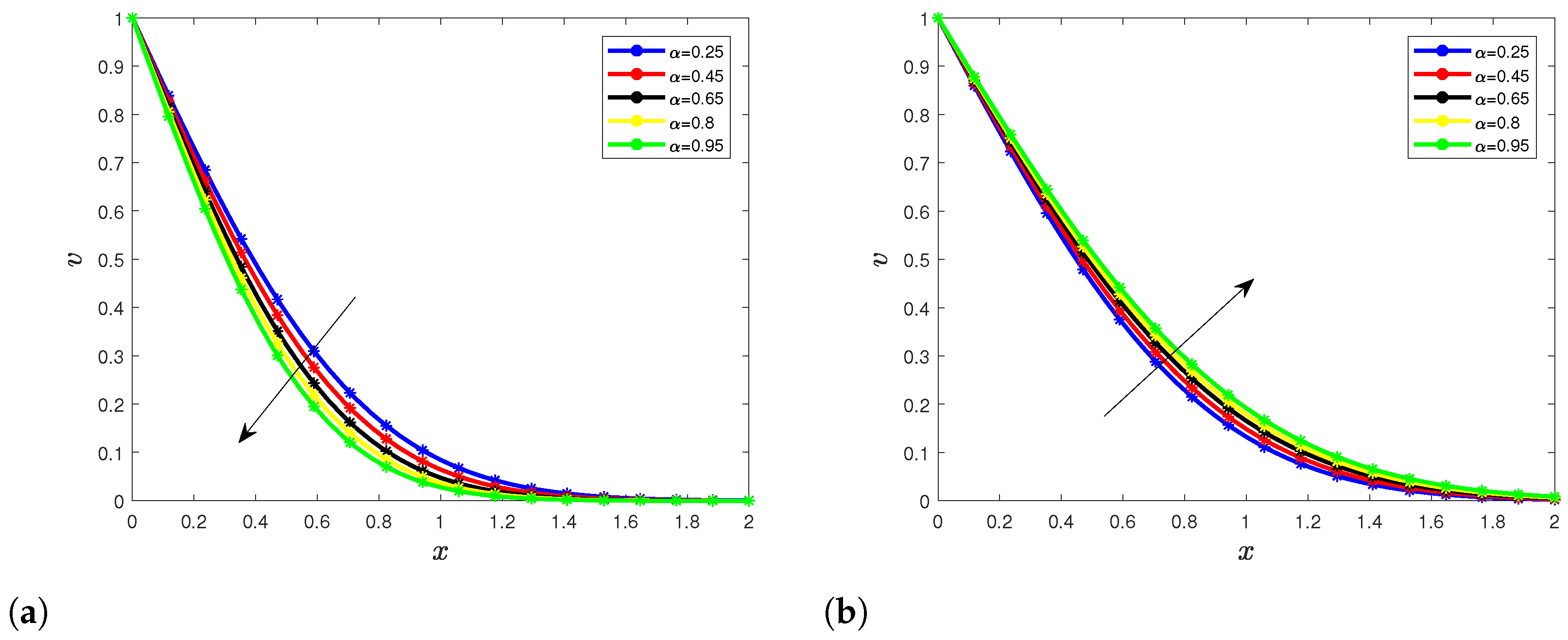
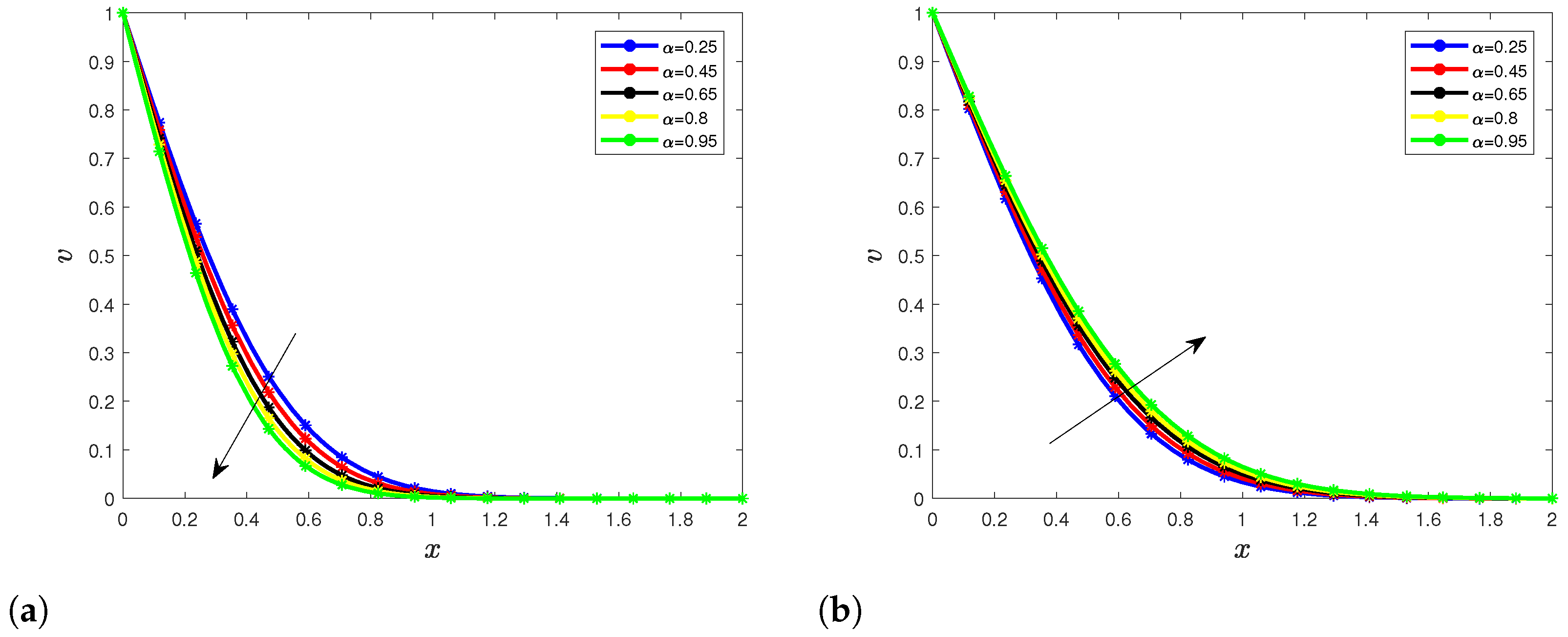
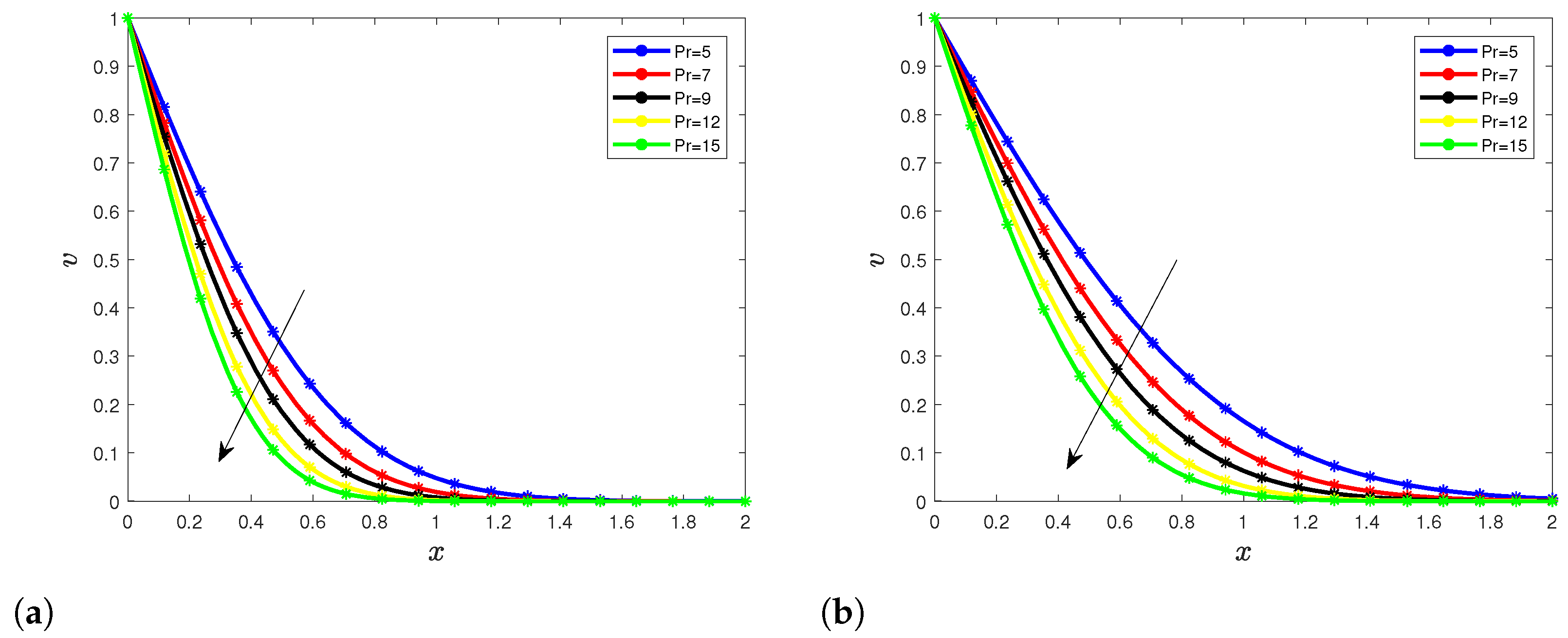
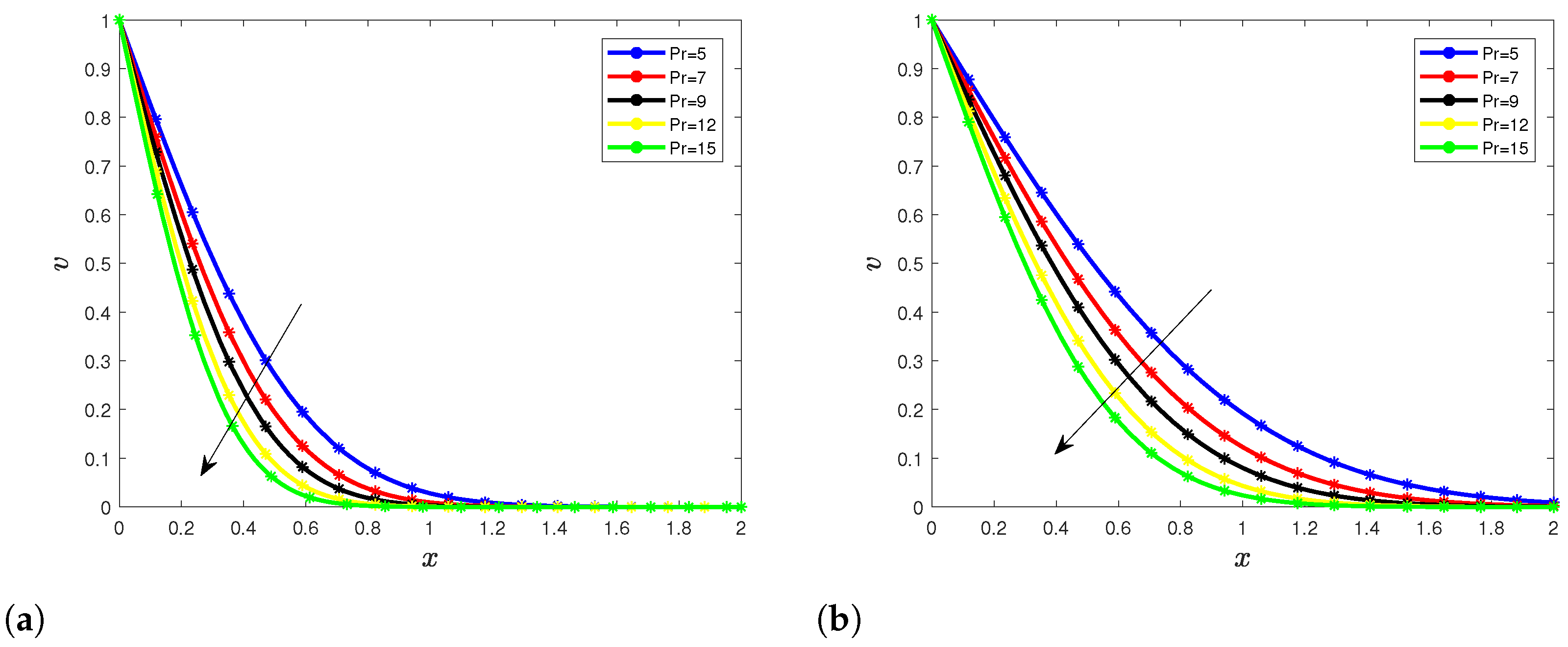
5.1. Temperature Profile

We begin our analysis with the heat Equation (15), whose solution is represented in Equation (25). For the figures in this section, Equation (25) has been considered. In the first dynamics, we consider different values of the order of the Caputo derivative and τ = 0.5 and τ = 1.5 . Without losing generality, we suppose that P r = 1 and P r = 5 , respectively. The figures are represented in the following Figure 1a,b and Figure 2a,b.
In Figure 1a and Figure 2a, we can observe when the considered time is τ = 0.5 ; in this case, when the order of the Caputo derivative increases, the dynamics of the fractional heat equation decrease as well. This means that when the considered time is less than 1, the Caputo derivative has an acceleration effect in the diffusion process. The arrow indicates the direction of the dynamics when the order increases. In Figure 1b and Figure 2b, the considered time is τ = 1.5 ; the direction of the dynamics can be observed by the direction of the arrow, and we observe that when the order increases, the dynamics of the heat diffusion equation increase as well. The numerical values can confirm the behaviors; see the results in the Tables.
The values in the Table 1 and Table 2 also confirm the boundary conditions considered in the present paper. It is visible that when the order of the fractional operator varies at each considered time, the temperature distribution decrease as well. In case the influence of the order of the derivative cannot be observed with the figures, it is recommended to calculate the difference that exists between the temperature profiles as illustrated in the Table 1 and Table 2. At the beginning of the diffusion process, we can observe that the difference between the trajectories is zero but increases when the variable x increases. We notice changes after a certain x because the errors term decreases and converges to zero. Thus, the Caputo derivative has a retardation effect in the diffusion processes. The differences in Table 1 and Table 2 are represented in Figure 3.
We now continue with the impact of the number P r . We consider different values of the P r numbers at two different times: τ = 0.5 and τ = 1.5 . The order of the fractional derivative is fixed to α = 0.65 and α = 0.95 , and the figures are represented as follows: Figure 4a,b and Figure 5a,b.
In Figure 4a and Figure 5a with τ = 0.5 and Figure 4b and Figure 5b with τ = 1.5 , the arrow indicates the direction of the dynamics when the P r number increases; we can observe, in both cases, that the influence of the P r number does not change. The increase in the P r number implies a decrease in the dynamics of the heat differential Equation (15). This finding can be explained by the fact greater values of this number reduce the heat temperature.

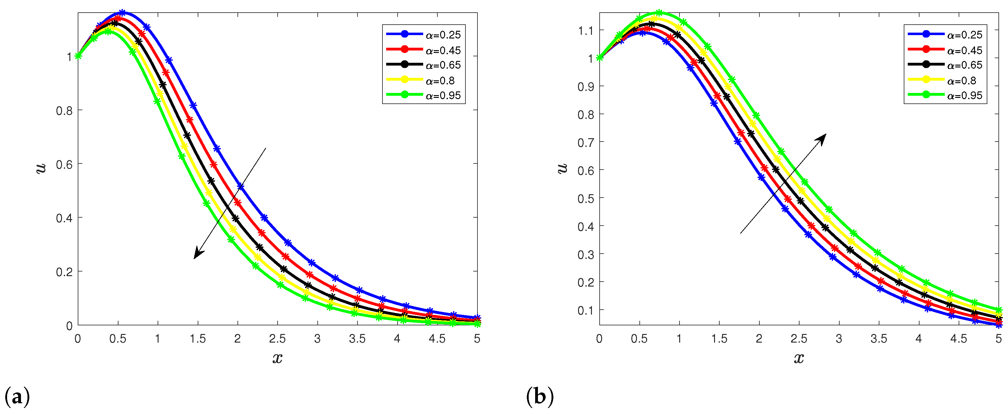
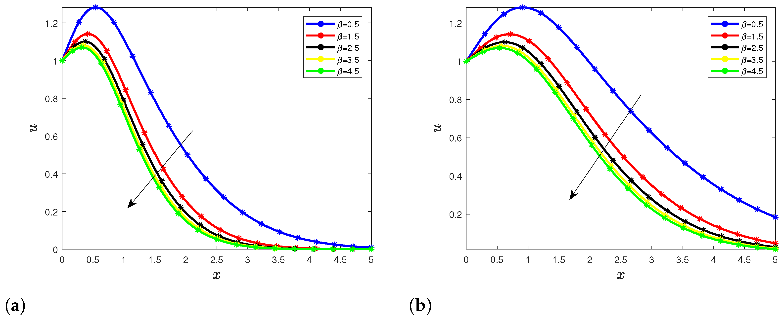
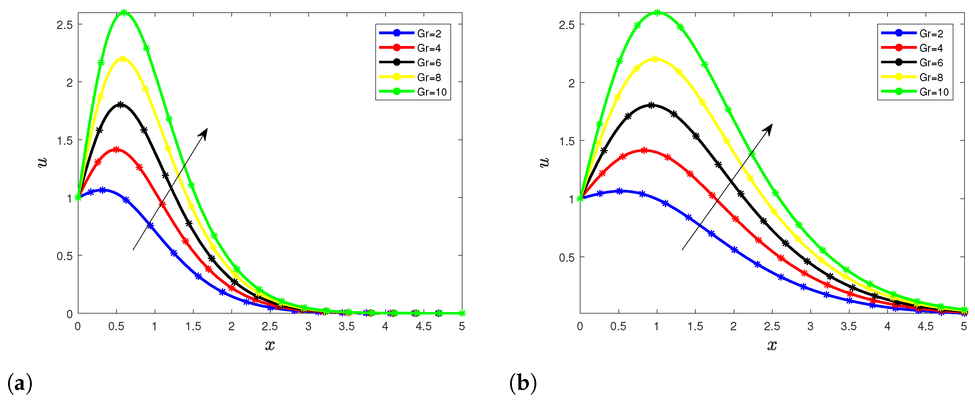
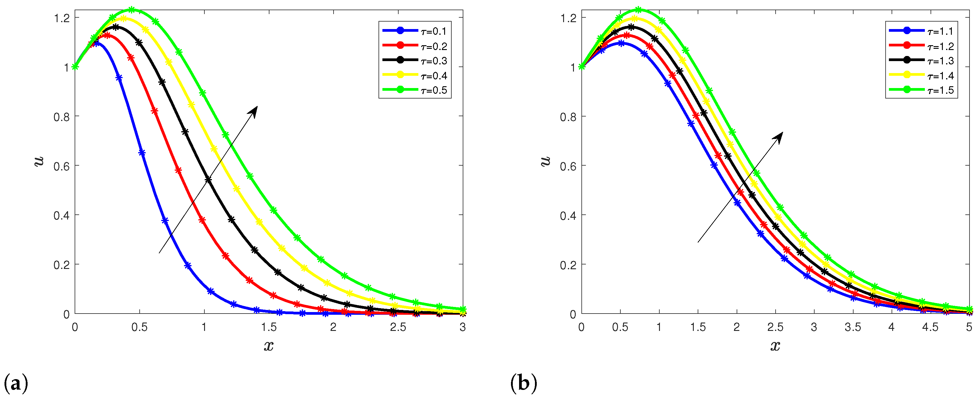
5.2. Velocity Profile

We now represent the dynamics of the velocity for different values of the fractional-order derivative at two different times τ = 0.5 and τ = 1.5 . In all figures in this section, Equation (39) has been considered. We consider β = 0.5 . The thermal grashof G r and the Prandtl number P r are assumed to be fixed in this part. We consider P r = 5 number and G r = 2 in this section for the graphical representations. We have the following Figure 6a,b.
When the time is τ = 0.5 in Figure 6a, we notice that when the order of the Caputo operator increases, then the velocity decreases following the arrow in this figure. That is, the order α of the Caputo derivative accelerates the decrease of the velocity to zero. We notice opposite phenomena when the considered time is τ = 1.5 in Figure 6b. Here, the increase in the order generates an increase in the velocity. Thus, the fractional-order has a regulator role in the fluid model considered in this paper. The role of the fractional operator does not change in the temperature distribution and the velocity profile.
Let us analyze the impact of the parameter β in the dynamics. We consider different values of the parameter β . We fix the following numbers P r = 5 and G r = 2 , and the order of the derivative is considered as α = 0.65 and α = 0.95 . We represent the figures in the following Figure 7a,b.
We notice that when the values of β increase, the velocity decreases as well for considered times τ = 0.5 and τ = 1.5 . This can be explained by the fact when Casson fluid parameter increases, the velocity boundary layer thickness is reduced.
We finish with the variation of the thermal grashof G r . We consider fixing P r = 5 and the order of the Caputo derivative to α = 0.95 . Referring to Equation (14), it is not hard to see for that all considered orders of the Caputo derivative when the parameter G r increases, it will generate an increase of the velocity. See the illustration in the following Figure 8a,b.
The increase of the velocity can be explained by the fact that when the thermal grashof G r increases, the difference of the temperature generated by the fractional heat equation increases as well, caused the augmentation of the velocity of the Casson fluid. Furthermore, when we combine these variations with the variation of the order of the Caputo derivative, it is normal for the velocity to increase as well.
Time also has an influence on the dynamics. We can notice that when the time increases, the velocity of the model increases too. This increase in the velocity is illustrated in the following Figure 9a,b.
The arrows in Figure 9a,b provide the directions generated by the impact of the time.
The present paper contributed to the application of the Caputo derivative to the model fluids model and to finding their exact analytical model. Note that the Caputo derivative nowadays has many domains of application, as in fractional-order neurons for parameter estimate [35], fractional viscoelasticity model described by fractional-order operators [36,37], fractional single-phase-lag model of heat conduction [38], and eigenproblem of molecular alignment and many others domains. The present investigations can be compared with the investigation by Ali et al. in [39], where the same model has been considered with different initial and boundaries conditions. In their investigation, the authors proposed the analytical solution using Laplace transform. We can observe that the results in [39] are in good agreement with the findings of the present investigations. In our present investigations, the novelty is we have used the combination between the Laplace transform and the Fourier sine transforms to get our solutions. Note that in these two works, the initial and boundaries conditions for the temperature and the velocity distributions in the constructive equations have minor differences. Note that the initial and boundaries conditions considered in this paper are particular cases of the initial and boundaries conditions considered in [39]. We consider the particular cases because the combination between the Laplace transform and the Fourier sine transform is not trivial when applied directly to the initial and boundaries conditions described in Equation (9) in [39].

6. Conclusions

In this paper, we have presented and illustrated the Laplace transform and the Fourier sine transform to solve the constructive equations presented in our paper. Many findings have been given. We notice that the fractional-order derivative has an retardation or acceleration effect on the heat equation. The parameter G r generates a retardation effect on the velocity of the model presented in this paper. Depending on the time considered, the order of the Caputo derivate can cause an increase in the velocity or a decrease in the velocity. Future research is needed to investigate the same problem using the fractional derivative with a non-singular derivative.

Funding

This research received no external funding.

Data Availability Statement

Not applicable.

Conflicts of Interest

The author declares that he has no conflict of interest.

References

  1. Atangana, A.; Araz, S.I. Extension of Atangana-Seda numerical method to partial differential equations with integer and non-integer order. Alex. Eng. J. 2020, 59, 2355–2370. [Google Scholar] [CrossRef]
  2. Qurashi, M.M.A.; Korpinar, Z.; Baleanu, D.; Inc, M. A new iterative algorithm on the time-fractional Fisher equation: Residual power series method. Adv. Mech. Eng. 2017, 9, 1–8. [Google Scholar] [CrossRef] [Green Version]
  3. Avci, D.; Yavuz, M.; Ozdemir, N. Fundamental Solutions to the Cauchy and Dirichlet Problems for a Heat Conduction Equation Equipped with the Caputo–Fabrizio Differentiation; Nova Science Publishers: Hauppauge, NY, USA, 2019; pp. 95–107. [Google Scholar]
  4. Lohana, B.; Abro, K.A.; Shaikh, A.W. Thermodynamical analysis of heat transfer of gravity-driven fluid flow via fractional treatment: An analytical study. J. Therm. Anal. Calorim. 2021, 144, 155–165. [Google Scholar] [CrossRef]
  5. Ali, F.; Sheikh, N.A.; Khan, I.; Saqib, M. Magnetic field effect on blood flow of Casson fluid in axisymmetric cylindrical tube: A fractional model. J. Magn. Magn. Mater. 2017, 423, 327–336. [Google Scholar] [CrossRef]
  6. Birajdar, G.A. An Implicit Numerical Method for Semilinear Space-Time Fractional Diffusion Equation. Dyn. Contin. Discret. Impuls. Syst. Ser. A Math. Anal. 2020, 27, 209–217. [Google Scholar]
  7. Birajdar, G.A. A New Approach for Non-linear Fractional Heat Transfer Model by Adomian Decomposition Method. In Mathematical Analysis and Computing. ICMAC 2019; Mohapatra, R.N., Yugesh, S., Kalpana, G., Kalaivani, C., Eds.; Springer Proceedings in Mathematics & Statistics; Springer: Berlin/Heidelberg, Germany, 2021; Volume 344. [Google Scholar]
  8. Khalil, R.; Horani, M.A.; Yousef, A.; Sababheh, M. A new definition of fractional derivative. J. Comput. Appl. Math. 2014, 264, 65–70. [Google Scholar] [CrossRef]
  9. Kilbas, A.A.; Srivastava, H.M.; Trujillo, J.J. Theory and Applications of Fractional Differential Equations; North-Holland Mathematics Studies; Elsevier: Amsterdam, The Netherlands, 2006; p. 204. [Google Scholar]
  10. Podlubny, I. Fractional Differential Equations; Mathematics in Science and Engineering; Academic Press: New York, NY, USA, 1999; p. 198. [Google Scholar]
  11. Atangana, A.; Baleanu, D. New fractional derivatives with nonlocal and non-singular kernel: Theory and application to heat transfer model. Therm. Sci. 2016, 20, 763–769. [Google Scholar] [CrossRef] [Green Version]
  12. Fahd, J.; Abdeljawad, T.; Baleanu, D. On the generalized fractional derivatives and their Caputo modification. J. Nonlinear Sci. Appl. 2017, 10, 2607–2619. [Google Scholar]
  13. Fahd, J.; Abdeljawad, T. Generalized fractional derivatives and Laplace transform. Discret. Contin. Dyn. Syst.-S 2019, 13, 709–722. [Google Scholar]
  14. Wang, X.; Wang, Z. Dynamic Analysis of a Delayed Fractional-Order SIR Model with Saturated Incidence and Treatment Function. Int. J. Bifurc. Chaos 2018, 28, 1850180. [Google Scholar] [CrossRef]
  15. Owolabi, K.M.; Atangana, A. On the formulation of Adams-Bashforth scheme with Atangana-Baleanu-Caputo fractional derivative to model chaotic problems. Chaos 2019, 29, 023111. [Google Scholar] [CrossRef]
  16. Hahn, D.W.; Özişik, M.N. Heat Conduction, 3rd ed.; John Wiley & Sons, Inc.: Hoboken, NJ, USA, 2020. [Google Scholar]
  17. Imran, M.A.; Shah, N.A.; Khan, I.; Aleem, M. Applications of non-integer Caputo time fractional derivatives to natural convection flow subject to arbitrary velocity and Newtonian heating. Neural Comput. Appl. 2018, 30, 1589–1599. [Google Scholar] [CrossRef]
  18. Khalid, A.; Khan, I.; Khan, A.; Shafie, S. Unsteady MHD free convection flow of Casson fluid past over an oscillating vertical plate embedded in a porous medium. Eng. Sci. Technol. Int. J. 2015, 18, 309–317. [Google Scholar] [CrossRef] [Green Version]
  19. Khan, A.; Abro, K.A.; Tassaddiq, A.; Khan, I. Atangana-Baleanu and Caputo Fabrizio analysis of fractional derivatives for heat and mass transfer of second grade fluids over a vertical plate: A comparative study. Entropy 2017, 19, 279. [Google Scholar] [CrossRef] [Green Version]
  20. Pramanik, S. Casson fluid flow and heat transfer past an exponentially porous stretching surface in presence of thermal radiation. Ain Shams Eng. J. 2014, 5, 205–212. [Google Scholar] [CrossRef] [Green Version]
  21. Abro, K.A. A Fractional and Analytic Investigation of Thermo-Diffusion Process on Free Convection Flow: An Application to Surface Modification Technology. Eur. Phys. J. Plus 2019, 135, 31–45. [Google Scholar] [CrossRef]
  22. Sene, N. Second-grade fluid model with Caputo-Liouville generalized fractional derivative. Chaos Solitons Fractals 2020, 133, 109631. [Google Scholar] [CrossRef]
  23. Sheikh, N.A.; Ali, F.; Saqib, M.; Khan, I.; Jan, S.A.A. A comparative study of Atangana-Baleanu and Caputo–Fabrizio fractional derivatives to the convective flow of a generalized Casson fluid. Eur. Phys. J. Plus 2017, 132, 54. [Google Scholar] [CrossRef]
  24. Abro, K.A.; Atangana, A. A comparative study of convective fluid motion in rotating cavity via Atangana–Baleanu and Caputo–Fabrizio fractal–fractional differentiations. Eur. Phys. J. Plus 2020, 135, 226. [Google Scholar] [CrossRef]
  25. Ali, F.; Saqib, M.; Khan, I.; Sheikh, N.A. Application of Caputo–Fabrizio derivatives to MHD free convection flow of generalized Walters’-B fluid model. Eur. Phys. J. Plus 2016, 131, 377. [Google Scholar] [CrossRef]
  26. Sene, N. Integral Balance Methods for Stokes’ First Equation Described by the Left Generalized Fractional Derivative. Physics 2019, 1, 154–166. [Google Scholar] [CrossRef] [Green Version]
  27. Khan, I.; Shah, N.A.; Vieru, D. Unsteady flow of generalized Casson fluid with fractional derivative due to an infinite plate. Eur. Phys. J. Plus 2016, 131, 181. [Google Scholar] [CrossRef]
  28. Shen, F.; Tan, W.; Zhao, Y.; Masuoka, T. The Rayleigh-Stokes problem for a heated generalized second grade fluid with fractional derivative model. Nonlinear Anal. Real World Appl. 2006, 7, 1072–1080. [Google Scholar] [CrossRef]
  29. Caputo, M.; Fabrizio, M. A new definition of fractional derivative without singular kernel. Progr. Fract. Differ. Appl. 2015, 1, 1–15. [Google Scholar]
  30. Sheikh, N.A.; Ali, F.; Saqib, M.; Khan, I.; Jan, S.A.A.; Alshomrani, A.S.; Alghamdi, M.S. Comparison and analysis of the Atangana–Baleanu and Caputo–Fabrizio fractional derivatives for generalized Casson fluid model with heat generation and chemical reaction. Results Phys. 2017, 7, 789–800. [Google Scholar] [CrossRef]
  31. Sene, N. A Numerical Algorithm Applied to Free Convection Flows of the Casson Fluid along with Heat and Mass Transfer Described by the Caputo Derivative. Adv. Math. Phys. 2021, 2021, 5225019. [Google Scholar] [CrossRef]
  32. Sene, N. Stokes’ first problem for heated flat plate with Atangana–Baleanu fractional derivative. Chaos Solitons Fractals 2018, 117, 68–75. [Google Scholar] [CrossRef]
  33. Sene, N. Analysis of the fractional diffusion equations described by Atangana-Baleanu-Caputo fractional derivative. Chaos Solitons Fractals 2019, 127, 158–164. [Google Scholar] [CrossRef]
  34. Sene, N. Analytical solutions and numerical schemes of certain generalized fractional diffusion models. Eur. Phys. J. Plus 2019, 134, 199. [Google Scholar] [CrossRef]
  35. Fazzino, S.; Caponetto, R.; Patane, C. A new model of Hopfield network with fractional-order neurons for parameter estimation. Nonlinear Dyn. Vol. 2021, 104, 2671–2685. [Google Scholar] [CrossRef]
  36. Mashayekhi, S.; Miles, P.; Hussainia, M.Y.; Oates, W.S. Fractional viscoelasticity in fractal and non-fractal media: Theory, experimental validation, and uncertainty analysis. J. Mech. Phys. Solids 2018, 111, 134–156. [Google Scholar] [CrossRef]
  37. Bonfanti, A.; Kaplan, J.L.; Charras, G.; Kabla, A. Fractional viscoelastic models for power-law materials. Soft Matter 2020, 16, 6002–6020. [Google Scholar] [CrossRef] [PubMed]
  38. Mishra, T.N.; Rai, K.N. Fractional single-phase-lagging heat conduction model for describing anomalous diffusion. Propuls. Power Res. 2016, 5, 45–54. [Google Scholar] [CrossRef] [Green Version]
  39. Ali, F.; Sheikh, N.A.; Khan, I.; Saqib, M. Solutions with Wright Function for Time Fractional Free Convection Flow of Casson Fluid. Arab. J. Sci. Eng. 2017, 42, 2565–2572. [Google Scholar] [CrossRef]
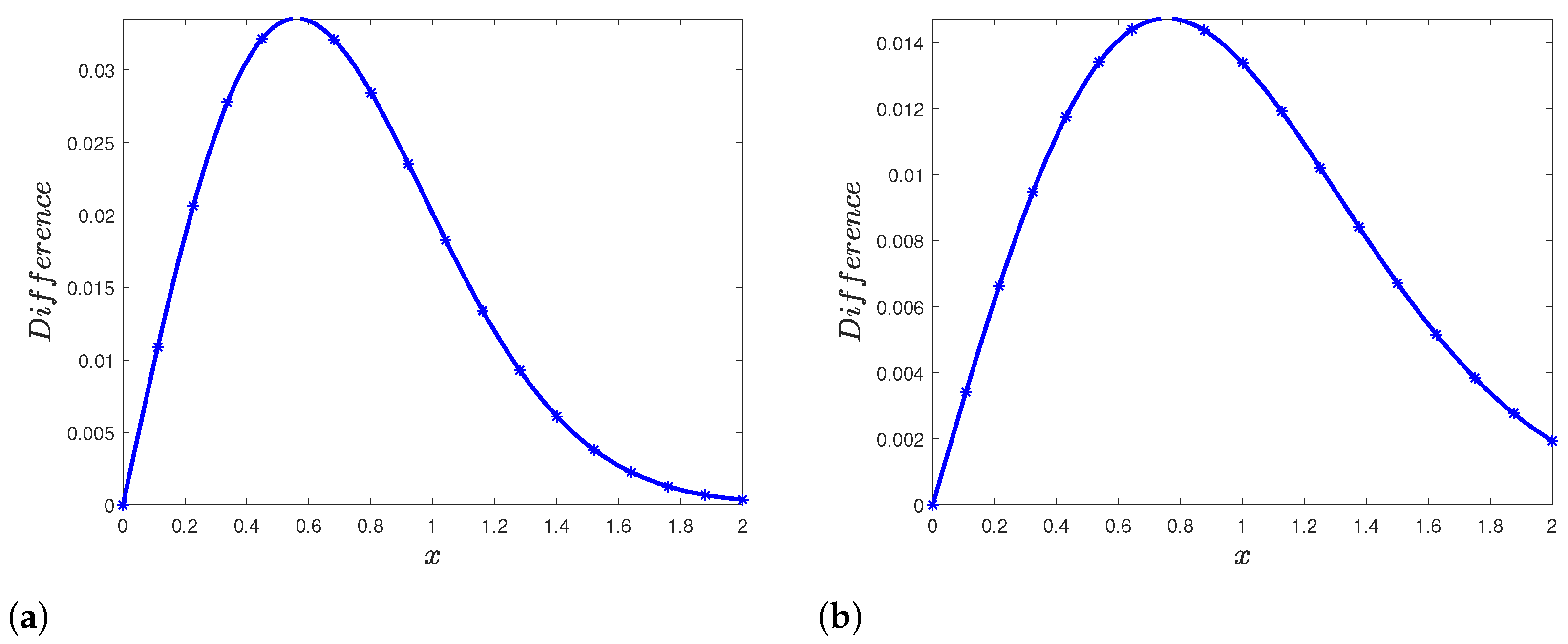
Figure 1. Dynamics of the fractional heat equation with various orders with respectively τ = 0.5 (a) and τ = 1.5 (b) for P r = 1 .
Fractalfract 06 00035 g001
Figure 2. Dynamics of the fractional heat equation with various order with, respectively, τ = 0.5 (a) and τ = 1.5 (b) for P r = 5 .
Fractalfract 06 00035 g002
Figure 3. Fractional-order influence in Table 1 (a) and Table 2 (b).
Fractalfract 06 00035 g003
Figure 4. Dynamics of the fractional heat equation with various orders with, respectively, τ = 0.5 (a) and τ = 1.5 (b) with α = 0.65 .
Fractalfract 06 00035 g004
Figure 5. Dynamics of the fractional heat equation with various orders with, respectively, τ = 0.5 (a) and τ = 1.5 (b) with α = 0.95 .
Fractalfract 06 00035 g005
Figure 6. Dynamics of the fractional diffusion reaction equation with various orders with, respectively, τ = 0.5 (a) and τ = 1.5 (b) with β = 0.5.
Fractalfract 06 00035 g006
Figure 7. Dynamics of the fractional diffusion reaction equation with various orders with, respectively, τ = 0.5 (a) with α = 0.65 and τ = 1.5 (b) with β = 0.95.
Fractalfract 06 00035 g007
Figure 8. Dynamics of the fractional diffusion reaction equation with various orders with, respectively, τ = 0.5 (a) and τ = 1.5 (b) with Pr = 5.
Fractalfract 06 00035 g008
Figure 9. Dynamics of the fractional diffusion reaction equation with various orders with, respectively, τ = 0.5 (a) and τ = 1.5 (b).
Fractalfract 06 00035 g009
Table 1. Temperature profile with P r = 1 .
x v ( x , τ ) at α = 0.25 and τ = 0.5 v ( x , τ ) at α = 0.45 and τ = 0.5 Difference ( . )
0.01.01.00
0.11760.83920.82780.0114
0.23530.68480.66350.0213
0.35290.54260.5140.0286
0.47060.41680.38420.03826
0.58920.30940.27590.0335
0.70590.22320.19170.0315
0.82350.15520.12760.0276
0.94120.10420.081520.02268
1.0590.067430.04990.01753
1.5290.00078590.0042030.0034171
Table 2. Temperature profile with P r = 5 .
x v ( x , τ ) at α = 0.8 and τ = 0.5 v ( x , τ ) at α = 0.95 and τ = 0.5 Difference ( . )
0.01.01.00
0.11760.87430.8780.0037
0.23530.75160.75880.0072
0.35290.6350.64510.0101
0.47060.52670.53920.0125
0.58920.4280.4420.014
0.70590.34230.35690.0146
0.82350.26790.28250.0146
0.94120.20530.21930.014
1.0590.15420.16690.0127
1.5290.039280.045610.00633
Publisher’s Note: MDPI stays neutral with regard to jurisdictional claims in published maps and institutional affiliations.

