Fractional Order Modeling the Gemini Virus in Capsicum annuum with Optimal Control

Abstract

In this article, a fractional model of the Capsicum annuum (C. annuum) affected by the yellow virus through whiteflies (Bemisia tabaci) is examined. We analyzed the model by equilibrium points, reproductive number, and local and global stability. The optimal control methods are discussed to decrease the infectious B. tabaci and C. annuum by applying the Verticillium lecanii (V. lecanii) with the Atangana–Baleanu derivative. Numerical results described the population of plants and comparison values of using V. lecanni. The results show that using 60% of V. lecanni will control the spread of the yellow virus in infected B. tabaci and C. annuum in 10 days, which helps farmers to afford the costs of cultivating chili plants.

1. Introduction

Growth of Capsicum annuum (chili plant) [1,2] is excessive in the mid-hill region of India. It contains vitamin C, provitamin A, and calcium, which are good for health. The spicy taste and high nutritional benefit the marketing of C. annuum. Capsicum annuum is used in the pharmaceutical industries to increase immunity, antiulcer, analgesic, antidiabetic, and antihemorrhoid agents. The extracts of C. annuum employ to relieve the pain of inflammation of joints, headaches, neuralgia, and burns. The framers require advantages to yield the C. annuum in large amounts. Due to natural obstacles like soil erosion, irrigation, and diseases spread, farmers encounter heavy losses while fertilizing C. annuum.

The cause of Geminivirus (yellow virus) [3,4,5] is one of the difficulties experienced by farmers in the cultivation of C. annuum. Yellow spots appear in young leaves and shoots, and the leaves turn out to be bright yellow or mixed yellow-green, which are symptoms of the yellow virus. This virus spreads by whitefly (Bemisia tabaci) from one host to another continuously.

Controlling these viruses using overlapping cropping methods is very difficult, since insecticide must be applied to mature plants. Controlling techniques vary depending on the conditions of the plants infected by virus variety, environment, and time. To reduce the populations of white-flies, systemic insecticides are applied to control the spread of the virus, as well as to cure the infected white-fly insect and plants, like rust fungi, etc., who have the host cyclodepsipeptide toxin. This toxin was produced via the mycelium of entomopathogenic fungi (Verticillium lecanii) [6,7,8]. However, the excess use of V. lecanii generates high costs. To minimize costs of controlling the B. tabaci population, an optimal control method must be found.

Over the past few decades, numerous analyses, real-world problems, and numerical methods were resolved by fractional derivatives and integrals [9,10,11,12,13,14,15,16]. The applications are fluid mechanics, electrochemistry, viscoelasticity, optics, and signals processing in engineering and science. Riemann–Liouville, Caputo, Caputo–Fabrizio, and Atangana–Baleanu are some of the fractional derivatives developed by several researchers. The Atangana–Baleanu fractional derivative (AB-derivative) [17] is a new one among the Mittag–Leffler Kernel. Recently, the existence analysis [18,19,20,21], stability analysis [22,23] and models [24,25,26,27] of AB-derivative were elaborated by many authors.

Optimal control is the approach of ascertaining control and circumstances path for dynamic systems to minimize an accomplishment period. The origin of the optimal control is related to the calculus of variations. In the 1940s, the formulation of dynamic programming in the optimal control was developed by Rochard Bellman. Using the analytical method, some of the optimal control problems’ solutions are difficult to find. N.H. Sweilam et al. [28] discussed the optimal control method for cancer treatment using AB-derivative. R. Amelia et al. [29] showed results to help farmers afford the costs of cultivating the red chilies by optimal control. In [30] N.H. Sweilam and S.M. AL–Mekhlafi described the fractional model of multistrain TB cure with optimal control. The optimal control problems to solve numerical procedures were investigated in [31,32].

To the best of our knowledge, the study of the C. annuum of the yellow virus with optimal control by applying the AB-derivative to the model is yet to come. This article was organized as follows: the basic results and definitions of the AB-derivative are discussed in Section 2. In Section 3, the formation of the C. annuum model with AB-derivative is explained. In Section 4, the optimality conditions demonstrate. In Section 5 and Section 6, numerical results with graphs for the fractional optimal control problem have presented and conclusions.

Motivated by [22,23,28,30], this document discusses the fractional model of Geminivirus in C. annuum with AB-derivative via optimal control and stability analysis. The main contributions are organized as follows:

(A)

The fractional model of Geminivirus in C. annuum with AB-derivative constructed.

(B)

We obtained some stability results of this fractional model and discussed the equilibrium points and reproductive number of the model.

(C)

We derived the optimal control of this fractional model and plotted the population and comparison results of each variable in the model.

2. Preliminaries

This section briefly discussed some preliminaries regarding fractional derivatives. There are few definitions for the fractional derivatives, including Riemann–Liouville, Caputo, and Caputo–Fabrizio [9,18]. Recently, a new fractional derivative with Mittag–Leffler Kernel was elaborated and implemented in a few real-world models [24,25,26,27]. We present the following definitions.

The Riemann–Liouville fractional integral (RL) is defined as follows [9,18]

$$\begin{array}{c}\hfill \left({}_0{I}^{\zeta }\varphi \right)\left(t\right)=\frac{1}{\mathsf{\Gamma }\left(\zeta \right)}{\int }_0^t{(t-s)}^{\zeta -1}\varphi \left(s\right)ds,\zeta >0.\end{array}$$

The Riemann–Liouville fractional order derivative (RL) is defined as follows [9,18]

$$\begin{array}{c}\hfill \left({}_0^R{D}^{\zeta }\varphi \right)\left(t\right)=\frac{d}{dt}\left(\frac{1}{\mathsf{\Gamma }(1-\zeta )}{\int }_0^t{(t-s)}^{-\zeta }\varphi \left(s\right)ds\right),0<\zeta <1.\end{array}$$

The Caputo fractional order derivative (C) is defined as follows [9,18]

$$\begin{array}{c}\hfill \left({}_0^C{D}^{\zeta }\varphi \right)\left(t\right)=\frac{1}{\mathsf{\Gamma }(1-\zeta )}{\int }_0^t{(t-s)}^{-\zeta }{\varphi }^{{}^{\prime }}\left(s\right)ds,0<\zeta <1.\end{array}$$

The Caputo-Fabrizio fractional order derivative in Caputo sense (CFC) is defined as follows [33]

$$\begin{array}{c}\hfill \left({}_0^{CFC}{D}^{\zeta }\varphi \right)\left(t\right)=\frac{M\left(\zeta \right)}{1-\zeta }{\int }_0^t{\varphi }^{{}^{\prime }}\left(s\right)exp\left[\frac{-\zeta }{1-\zeta }{(t-s)}^{\zeta }\right]ds,0<\zeta <1.\end{array}$$

where ${\varphi }^{{}^{\prime }}\in H^1(0,T)$, $M\left(\zeta \right)$ is a constant of normalization that depends on $\zeta$, which satisfies that, $M\left(0\right)=M\left(1\right)=1.$

The Atangana–Baleanu fractional order derivative in the Riemann–Liouville sense (ABR) is defined as follows [17]

$$\begin{array}{c}\hfill \left({}_0^{ABR}{D}^{\zeta }\varphi \right)\left(t\right)=\frac{B\left(\zeta \right)}{1-\zeta }\frac{d}{dt}{\int }_0^t\varphi \left(s\right)E_{\zeta }\left[-\zeta \frac{{(t-s)}^{\zeta }}{1-\zeta }\right]ds,0<\zeta <1.\end{array}$$

where ${\varphi }^{{}^{\prime }}\in H^1(0,T)$, $B\left(\zeta \right)$ is a normalization function, $B\left(0\right)=B\left(1\right)=1$.

The Atangana–Baleanu fractional order derivative in the Caputo sense (ABC) is defined as follows [17]

$$\begin{array}{c}\hfill \left({}_0^{ABC}{D}^{\zeta }\varphi \right)\left(t\right)=\frac{B\left(\zeta \right)}{1-\zeta }{\int }_0^t{\varphi }^{{}^{\prime }}\left(s\right)E_{\zeta }\left[-\zeta \frac{{(t-s)}^{\zeta }}{1-\zeta }\right]ds,0<\zeta <1.\end{array}$$

where ${\varphi }^{{}^{\prime }}\in H^1(0,T)$, $B\left(\zeta \right)$ is a normalization function, $B\left(0\right)=B\left(1\right)=1$.

The Atangana–Baleanu fractional integral of order $\zeta$ of a function $\varphi \left(t\right)$ is defined as [17]

$$\begin{array}{c}\hfill \left({}_0^{AB}{I}^{\zeta }\varphi \right)\left(t\right)=\frac{1-\zeta }{B\left(\zeta \right)}\varphi \left(t\right)+\frac{\zeta }{B\left(\zeta \right)}\left({}_0^{}{I}^{\zeta }\varphi \right)\left(t\right).\end{array}$$

The Mittag–Leffler function of one and two parameters $E_{\alpha }\left(z\right),E_{\alpha ,\beta }\left(z\right)$ is defined as [9]

$$\begin{array}{cc}\hfill E_{\alpha }\left(z\right)& =\sum _{k=0}^{\infty }\frac{z^k}{\mathsf{\Gamma }(\alpha k+1)}z,\alpha \in C,Re\left(\alpha \right)>0.\hfill \\ \hfill E_{\alpha ,\beta }\left(z\right)& =\sum _{k=0}^{\infty }\frac{z^k}{\mathsf{\Gamma }(\alpha k+\beta )}z,\alpha ,\beta \in C,Re\left(\alpha \right)>0,Re\left(\beta \right)>0.\hfill \end{array}$$

The generalized Mittag–Leffler function is defined as [9]

$$\begin{array}{c}\hfill E_{\alpha ,\beta }^{\gamma }\left(z\right)=\sum _{k=0}^{\infty }\frac{{\left(\gamma \right)}_n}{\mathsf{\Gamma }(\alpha k+\beta )}\frac{z^k}{k!}z,\alpha ,\beta ,\gamma \in C,Re\left(\alpha \right)>0,Re\left(\beta \right)>0,Re\left(\gamma \right)>0,\end{array}$$

where $\mathsf{\Gamma }(·)$ denotes the Gamma function, and note that

$$\begin{array}{c}\hfill E_{1,1}^1\left(z\right)=e^z,E_{\alpha ,1}^1\left(z\right)=E_{\alpha }\left(z\right),E_{\alpha ,\beta }^1\left(z\right)=E_{\alpha ,\beta }\left(z\right).\end{array}$$

3. Modeling Framework of Gemini Virus

The fractional model based on the cure of yellow virus in C. annuum by V. lecanii with modified variables and parameters is presented. Here, the parameters depend on the fractional model, which is an extension of the integer model given in [29]. The mathematical model of C. annuum with AB fractional derivative is represented as follows:

$$\begin{array}{c}\hfill \left.\begin{array}{cc}\hfill \left({}_0^{ABC}{D}_t^{\zeta }\right)\left(S_v\left(t\right)\right)& =A-\alpha S_v-{\beta }_1(1-{\delta }_p)S_v{I}_{BT}-{\mu }_p{S}_v\hfill \\ \hfill \left({}_0^{ABC}{D}_t^{\zeta }\right)\left(I_v\left(t\right)\right)& ={\beta }_1(1-{\delta }_p)S_v{I}_{BT}-{\mu }_p{I}_v\hfill \\ \hfill \left({}_0^{ABC}{D}_t^{\zeta }\right)\left(S_g\left(t\right)\right)& =\alpha S_v-{\beta }_2(1-{\delta }_p)S_g{I}_{BT}-{\mu }_p{S}_g\hfill \\ \hfill \left({}_0^{ABC}{D}_t^{\zeta }\right)\left(I_g\left(t\right)\right)& ={\beta }_2(1-{\delta }_p)S_g{I}_{BT}-{\mu }_p{I}_g\hfill \\ \hfill \left({}_0^{ABC}{D}_t^{\zeta }\right)\left(S_{BT}\left(t\right)\right)& =B{N}_v-{\gamma }_1(1-{\delta }_p)I_v{S}_{BT}-{\gamma }_2(1-{\delta }_p)I_g{S}_{BT}\hfill \\ & -{\theta }_1{\delta }_p{S}_{BT}{N}_p-{\mu }_1{S}_{BT}\hfill \\ \hfill \left({}_0^{ABC}{D}_t^{\zeta }\right)\left(I_{BT}\left(t\right)\right)& ={\gamma }_1(1-{\delta }_p)I_v{S}_{BT}+{\gamma }_2(1-{\delta }_p)I_g{S}_{BT}\hfill \\ & -{\theta }_1{\delta }_p{I}_{BT}{N}_p-{\mu }_1{I}_{BT}\hfill \\ \hfill \mathrm{with}{S}_v\left(0\right)& =S_{v0},I_v\left(0\right)=I_{v0},\hfill \\ \hfill S_g\left(0\right)& =S_{g0},I_g\left(0\right)=I_{g0},\hfill \\ \hfill S_{BT}\left(0\right)& =S_{BT0},I_{BT}\left(0\right)=I_{BT0},\hfill \end{array}\right\}\end{array}$$

(1)

where $0<\zeta <1$.

The total population is denoted by $N_p$ of C. annuum $N_p=S_v+I_v+S_g+I_g$ is taken to be constant. The total population of B. tabaci is denoted by $N_v=S_{BT}+I_{BT}$. Here, the total population can be divided into 6 subgroups.

•

$S_v$ denotes a set of noninfected C. annuum in vegetative phase liable to possible infection.

•

$I_v$ denotes a set of infected C. annuum in vegetative phase.

•

$S_g$ denotes a set of noninfected C. annuum in generative phase liable to possible infection.

•

$I_g$ denotes a set of infected C. annuum in generative phase.

•

$S_{BT}$ denotes a set of noninfected B. tabaci(white bug) liable to possible infection.

•

$I_{BT}$ denotes a set of infected B. tabaci.

The recruitment rate of C. annuum and B. tabaci is denoted by A and B respectively. The growth rate of C. annuum from vegetative to generative phase is denoted by $\alpha$. ${\beta }_1$, and ${\beta }_2$ denoted the infection rate of C. annuum in the vegetative and generative phase respectively. ${\gamma }_1$, and ${\gamma }_2$ denoted the infection rate of B. tabaci in the vegetative and generative phase respectively. ${\delta }_p$ stands for the rate of use of V. lecanii. The death rate of C. annuum is denoted by ${\mu }_p$. The natural death rate of B. tabaci is denoted by ${\mu }_1$, and the death rate of B. tabaci due to curative intervention is denoted by ${\theta }_1$.

4. Basic Analysis of the Model

4.1. Invariant Region

The fractional order C. annuum model of yellow virus (1) can be analyzed in the biological feasible region discussed as follows. The system (1) is split into two parts, namely the C. annuum population $(N_p;\mathrm{with}{N}_p=S_v+I_v+S_g+I_g)$ and the B. tabaci population $(N_v;\mathrm{with}{N}_v=S_{BT}+I_{BT})$.

Let the feasible region $F=F_p\cup F_v\subset R_{+}^4\times R_{+}^2$ with

$$\begin{array}{cc}\hfill F_p& =\left\{(S_v,I_v,S_g,I_g)\in R_{+}^4:S_v+I_v+S_g+I_g\le \frac{A}{{\mu }_p}\right\},\hfill \\ \hfill F_v& =\left\{(S_{BT},I_{BT})\in R_{+}^2:S_{BT}+I_{BT}\le \frac{B}{{\theta }_1{\delta }_p{N}_p+{\mu }_1}\right\}.\hfill \end{array}$$

To establish the positive invariance of $F〈\mathrm{i}.\mathrm{e}.,\mathrm{solutions}\mathrm{in}F\mathrm{remain}\mathrm{in}F\mathrm{for}\mathrm{all}t>0〉$. Adding the first four equations and the last two equations of the model (1) gives

$$\begin{array}{cc}\hfill {}_0^{ABC}{D}_t^{\zeta }{N}_p\left(t\right)& =A-{\mu }_p(S_v+I_v+S_g+I_g)=A-{\mu }_p{N}_p\hfill \end{array}$$

(2)

$$\begin{array}{cc}\hfill \hspace{1em}\hspace{1em}\hspace{1em}{}_0^{ABC}{D}_t^{\zeta }{N}_v\left(t\right)& =B{N}_v-({\theta }_1{\delta }_p{N}_p+{\mu }_1)N_v=B-({\theta }_1{\delta }_p{N}_p+{\mu }_1)N_v\hfill \end{array}$$

(3)

This can be used to show that the fractional order of the C. annuum and B. tabaci population in the system (1) shows that

$$\begin{array}{c}\hfill \left.\begin{array}{cc}\hfill {}_0^{ABC}{D}_t^{\zeta }{N}_p\left(t\right)& \le A-{\mu }_p{N}_p,\hfill \\ \hfill {}_0^{ABC}{D}_t^{\zeta }{N}_v\left(t\right)& \le B-({\theta }_1{\delta }_p{N}_p+{\mu }_1)N_v.\hfill \end{array}\right\}\end{array}$$

(4)

which implies that

$$\begin{array}{cc}\hfill N_p\left(t\right)& \le A{t}^{\zeta }{E}_{\zeta ,\zeta +1}(-{\mu }_p{t}^{\zeta })-N_p\left(0\right)E_{\zeta ,1}(-{\mu }_p{t}^{\zeta }),\hfill \\ \hfill N_v\left(t\right)& \le B{t}^{\zeta }{E}_{\zeta ,\zeta +1}(-({\theta }_1{\delta }_p{N}_p+{\mu }_1)t^{\zeta })+N_v\left(0\right)E_{\zeta ,1}(-({\theta }_1{\delta }_p{N}_p+{\mu }_1)t^{\zeta }).\hfill \end{array}$$

From above inequality, we observe that $N_p\left(t\right)\le \frac{A}{{\mu }_p}$ & $N_v\left(t\right)\le \frac{B}{({\theta }_1{\delta }_p{N}_p+{\mu }_1)}$. Thus, the region F is positively-invariant.

Hence, it is sufficient to consider the dynamics model of system (1) in F. The mathematical model is well-posed in the region F.

∴ Every solution of the basic model (1) with initial conditions in F remains in F for all $t>0$. The result is summarized below.

Lemma 1.

The region $F=F_p\cup F_v\subset R_{+}^4\times R_{+}^2$ is positively invariant for the basic model (1) with non-negative initial conditions in $R_{+}^6$.

4.2. Disease-Free Equilibrium Point

To evaluate the equilibrium points

Let

$$\begin{array}{cc}\hfill {}_0^{ABC}{D}_t^{\zeta }{S}_v\left(t\right)& =0,{}_0^{ABC}{D}_t^{\zeta }{S}_g\left(t\right)=0,{}_0^{ABC}{D}_t^{\zeta }{S}_{BT}\left(t\right)=0,\hfill \\ \hfill {}_0^{ABC}{D}_t^{\zeta }{I}_v\left(t\right)& =0,{}_0^{ABC}{D}_t^{\zeta }{I}_g\left(t\right)=0,{}_0^{ABC}{D}_t^{\zeta }{I}_{BT}\left(t\right)=0.\hfill \end{array}$$

Then

$$\begin{array}{c}\hfill {\mathcal{E}}_0(S_v^0,I_v^0,S_g^0,I_g^0,S_{BT}^0,I_{BT}^0)=\left(\frac{A}{{\mu }_p},0,0,0,\frac{B}{{\theta }_1{\delta }_p{N}_p+{\mu }_1},0\right).\end{array}$$

4.3. Reproduction Number

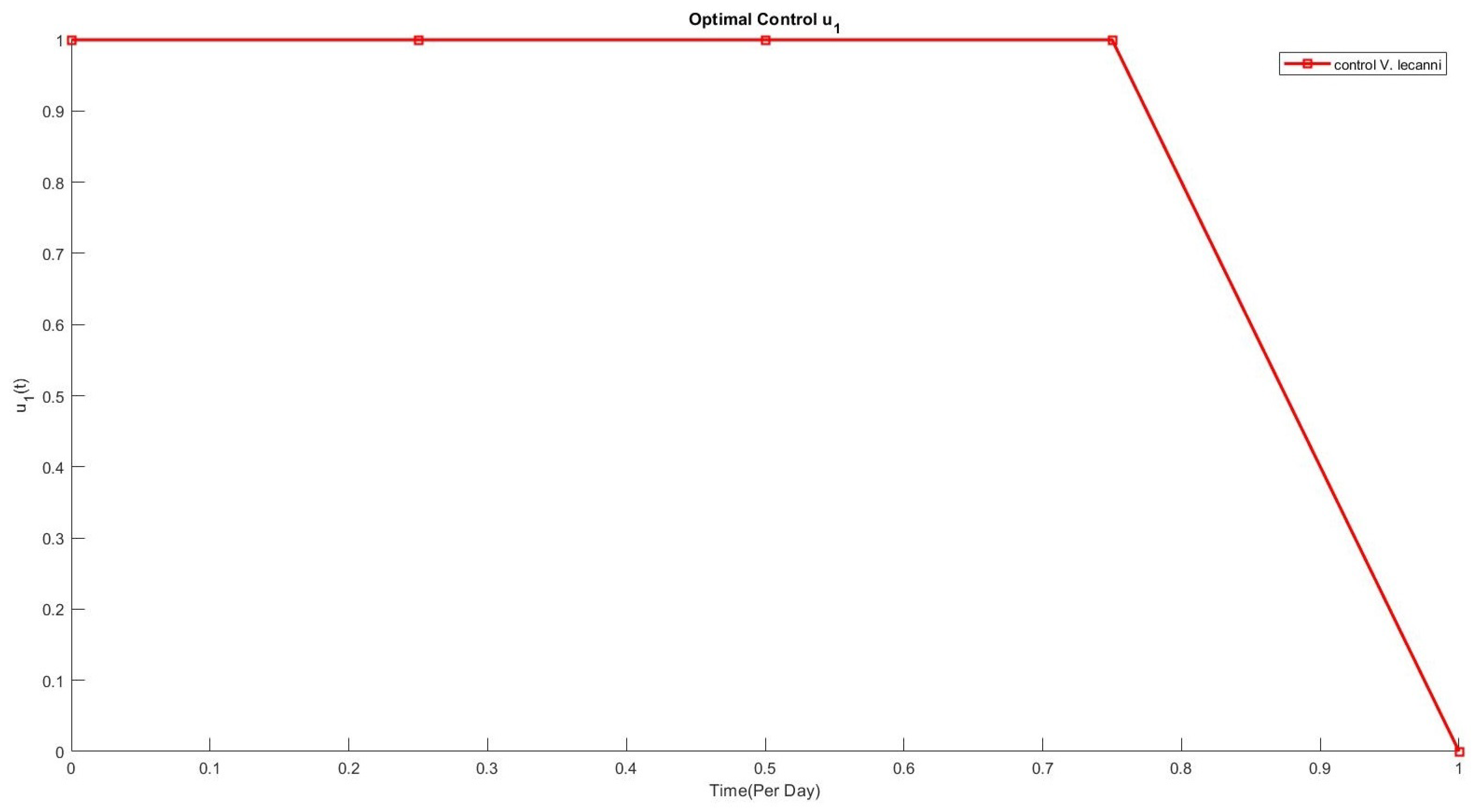
For the basic reproduction number for the C. annuum model (1), suppose that $y=(S_v,S_g,I_{BT})$ and using next generation matrix approach [34], we have

$$\begin{array}{c}\hfill \frac{dy}{dt}=\mathcal{F}\left(y\right)-\mathcal{V}\left(y\right),\end{array}$$

where Jacobian of $\mathcal{F}$ and $\mathcal{V}$ at ${\mathcal{E}}_0$, we have

$$\mathcal{F}=\left(\begin{array}{ccc}\alpha +{\mu }_p& 0& 0\\ -\alpha & {\mu }_p& 0\\ 0& 0& {\mu }_1\end{array}\right)\&\mathcal{V}=\left(\begin{array}{ccc}\frac{{\beta }_1(1-{\delta }_p)B}{{\theta }_1{\delta }_p{N}_p+{\mu }_1}& 0& \frac{{\beta }_1(1-{\delta }_p)A}{{\mu }_p}\\ 0& \frac{{\beta }_2(1-{\delta }_p)B}{{\theta }_1{\delta }_p{N}_p+{\mu }_1}& \frac{{\beta }_2(1-{\delta }_p)A}{{\mu }_p}\\ 0& 0& {\theta }_1{\delta }_p{N}_p\end{array}\right).$$

The basic reproduction number ${\psi }_0$ comes from the spectral radius ${\psi }_0=\rho \left[{\mathcal{FV}}^{-1}\right]$, given by

$$\begin{array}{c}\hfill {\psi }_0=\frac{(\alpha +{\mu }_p)({\theta }_1{\delta }_p{N}_p+{\mu }_1)}{{\beta }_1(1-{\delta }_p)B},\end{array}$$

where

$${\mathcal{FV}}^{-1}=\left(\begin{array}{ccc}\frac{(\alpha +{\mu }_p)({\theta }_1{\delta }_p{N}_p+{\mu }_1)}{{\beta }_1(1-{\delta }_p)B}& 0& 0\\ 0& \frac{{\mu }_p({\theta }_1{\delta }_p{N}_p+{\mu }_1)}{{\beta }_2(1-{\delta }_p)B}& 0\\ 0& 0& \frac{{\mu }_1}{{\theta }_1{\delta }_p{N}_p}\end{array}\right).$$

Theorem 1.

There exists a unique positive endemic equilibrium point ${\mathcal{E}}^{*}$ for system (1) if ${\psi }_0>1$.

Proof. 

Endemic equilibrium point is obtained from system (1), and by putting right-hand side of each equation equal to zero, we have

$$\begin{array}{cc}\hfill S_v^{*}& =\frac{A}{a}\hfill \\ \hfill I_v^{*}& =\frac{A{\beta }_1(1-{\delta }_p)I_{BT}}{{\mu }_{p}a}\hfill \\ \hfill S_g^{*}& =\frac{A\alpha }{ab}\hfill \\ \hfill I_g^{*}& =\frac{A\alpha {\beta }_2(1-{\delta }_p)I_{BT}}{{\mu }_{p}ab}\hfill \\ \hfill S_{BT}^{*}& =\frac{B{N}_v{\mu }_{p}ab}{{\gamma }_1(1-{\delta }_p^{2}A{\beta }_1)I_{BT}b+{\gamma }_2{\beta }_2\alpha A{(1-{\delta }_p)}^2{I}_{BT}+({\theta }_1{\delta }_p{N}_p-{\mu }_1){\mu }_{p}ab},\hfill \end{array}$$

where $a=\alpha +{\beta }_1(1-{\delta }_p)I_{BT}-{\mu }_p$ and $b={\beta }_2(1-{\delta }_p)I_{BT}+{\mu }_p$ and $I_{BT}^{*}$ is the positive root of $\mathcal{K}\left(I_{BT}\right)=i_5{I}_{BT}^5+i_4{I}_{BT}^4+i_3{I}_{BT}^3+i_2{I}_{BT}^2+i_1{I}_{BT}=0,$

where

$$\begin{array}{cc}\hfill i_1& ={({\theta }_1{\delta }_p{N}_p+{\mu }_1)}^2{\mu }_p^4(\alpha -{\mu }_p)[(\alpha -{\mu }_p)+2{\beta }_1(1-{\delta }_p)]\hfill \\ & -AB{N}_v({\gamma }_1{\beta }_1{\mu }_p^2+\alpha {\gamma }_2{\beta }_2{\mu }_p){(1-{\delta }_p)}^2[\alpha {\mu }_p-{\mu }_p^2],\hfill \\ \hfill i_2& =(A\alpha {\gamma }_1{\beta }_1{\mu }_p^2{(1-{\delta }_p)}^2-A{\gamma }_1{\beta }_1{\mu }_p^3{(1-{\delta }_p)}^2+A{\alpha }^2{\gamma }_2{\beta }_2{\mu }_p^2{(1-{\delta }_p)}^2-A\alpha {\gamma }_2{\beta }_2{\mu }_p^3{(1-{\delta }_p)}^2\hfill \\ & +2{\beta }_2({\theta }_1{\delta }_p{N}_p+{\mu }_1){\mu }_p^3{(\alpha -{\mu }_p)}^2(1-{\delta }_p))({\theta }_1{\delta }_p{N}_p+{\mu }_1)-AB{N}_v{\gamma }_1{\beta }_1{\beta }_2{\mu }_p{(1-{\delta }_p)}^3[\alpha {\mu }_p-{\mu }_p^2]\hfill \\ & -AB{N}_v({\gamma }_1{\beta }_1{\mu }_p^2+\alpha {\gamma }_2{\beta }_2{\mu }_p){(1-{\delta }_p)}^2[\alpha {\beta }_2(1-{\delta }_p)+{\mu }_p{\beta }_1(1-{\delta }_p)-{\mu }_p{\beta }_2(1-{\delta }_p)],\hfill \\ \hfill i_3& =(A\alpha {\gamma }_1{\beta }_1{\beta }_2{\mu }_p{(1-{\delta }_p)}^3+A{\gamma }_1{\beta }_1^2{\mu }_p{(1-{\delta }_p)}^3-A{\gamma }_1{\beta }_1{\beta }_2{\mu }_p^2{(1-{\delta }_p)}^3+A{\alpha }^2{\gamma }_2{\beta }_2^2{\mu }_p{(1-{\delta }_p)}^3\hfill \\ & +A\alpha {\gamma }_2{\beta }_1{\beta }_2{\mu }_p^2{(1-{\delta }_p)}^3-A\alpha {\gamma }_2{\beta }_2^2{\mu }_p^2{(1-{\delta }_p)}^3\hfill \\ & +({\theta }_1{\delta }_p{N}_p+{\mu }_1){\mu }_p^2\left[{\beta }_2^2{(\alpha -{\mu }_p)}^2{(1-{\delta }_p)}^2+4{\beta }_1{\beta }_2{\mu }_p{(1-{\delta }_p)}^2(\alpha -{\mu }_p)+{\beta }_1^2{\mu }_p^2{(1-{\delta }_p)}^2\right])\hfill \\ & \times ({\theta }_1{\delta }_p{N}_p+{\mu }_1)-AB{N}_v{\gamma }_1{\beta }_1{\beta }_2{\mu }_p{(1-{\delta }_p)}^3[\alpha {\beta }_2(1-{\delta }_p)+{\mu }_p{\beta }_1(1-{\delta }_p)-{\mu }_p{\beta }_2(1-{\delta }_p)]\hfill \\ & -AB{N}_v{\gamma }_1{\beta }_1^2{\beta }_2{\mu }_p^2{(1-{\delta }_p)}^4-AB{N}_v\alpha {\gamma }_2{\beta }_1{\beta }_2^2{\mu }_p{(1-{\delta }_p)}^4,\hfill \\ \hfill i_4& =(A{\gamma }_1{\beta }_1^2{\beta }_2{\mu }_p{(1-{\delta }_p)}^4+A\alpha {\gamma }_2{\beta }_1{\beta }_2^2{\mu }_p{(1-{\delta }_p)}^4\hfill \\ & +({\theta }_1{\delta }_p{N}_p+{\mu }_1){\mu }_p^2[2{\beta }_1{(1-{\delta }_p)}^3{\beta }_2^2(\alpha -{\mu }_p)+2{\mu }_p{\beta }_1^2{\beta }_2{(1-{\delta }_p)}^3])({\theta }_1{\delta }_p{N}_p+{\mu }_1)\hfill \\ & -AB{N}_v{\gamma }_1{\beta }_1^2{\beta }_2{\mu }_p{(1-{\delta }_p)}^5,\hfill \\ \hfill i_5& ={\beta }_1^2{\beta }_2^2{(1-{\delta }_p)}^4{({\theta }_1{\delta }_p{N}_p+{\mu }_1)}^2{\mu }_p^2.\hfill \end{array}$$

It is obvious from the values of $S_v^{*},I_v^{*},S_g^{*},I_g^{*},S_{BT}^{*}\&I_{BT}^{*}$ that there exists a unique positive endemic equilibrium point ${\mathcal{E}}^{*}$, if $\psi \left(0\right)>1$. □

Theorem 2.

The system (1) is locally stable at ${\mathcal{E}}_0$ for ${\psi }_0<1$ and unstable for ${\psi }_0>1$.

Proof. 

The Jacobian of system (1) is

$$J=\left(\begin{array}{cccccc}{Q}_1& 0& 0& 0& 0& \frac{-{\beta }_1(1-{\delta }_p)A}{{\mu }_p}\\ \frac{{\beta }_1(1-{\delta }_p)B}{{\theta }_1{\delta }_p{N}_p+{\mu }_1}& -{\mu }_p& 0& 0& 0& \frac{{\beta }_1(1-{\delta }_p)A}{{\mu }_p}\\ \alpha & 0& Q_2& 0& 0& \frac{-{\beta }_2(1-{\delta }_p)A}{{\mu }_p}\\ 0& 0& \frac{{\beta }_2(1-{\delta }_p)B}{{\theta }_1{\delta }_p{N}_p+{\mu }_1}& -{\mu }_p& 0& \frac{{\beta }_2(1-{\delta }_p)A}{{\mu }_p}\\ 0& \frac{-{\gamma }_1(1-{\delta }_p)B}{{\theta }_1{\delta }_p{N}_p+{\mu }_1}& 0& \frac{-{\gamma }_2(1-{\delta }_p)B}{{\theta }_1{\delta }_p{N}_p+{\mu }_1}& Q_3& 0\\ 0& \frac{{\gamma }_1(1-{\delta }_p)B}{{\theta }_1{\delta }_p{N}_p+{\mu }_1}& 0& \frac{{\gamma }_2(1-{\delta }_p)B}{{\theta }_1{\delta }_p{N}_p+{\mu }_1}& Q_4& Q_5\end{array}\right)$$

where

$$\begin{array}{cc}\hfill Q_1& =-[\alpha +{\mu }_p+{\beta }_1(1-{\delta }_p)I_{BT}],\hfill \\ \hfill Q_2& =-[{\mu }_p+{\beta }_2(1-{\delta }_p)I_{BT}],\hfill \\ \hfill Q_3& =-[{\gamma }_1(1-{\delta }_p)I_v+{\gamma }_2(1-{\delta }_p)I_g+{\theta }_1{\delta }_p{N}_p+{\mu }_1],\hfill \\ \hfill Q_4& ={\gamma }_1(1-{\delta }_p)I_v+{\gamma }_2(1-{\delta }_p)I_g,\hfill \\ \hfill Q_5& =-[{\theta }_1{\delta }_p{N}_p+{\mu }_1].\hfill \end{array}$$

Along ${\mathcal{E}}_0$, it implies that

$$J\left({\mathcal{E}}_0\right)=\left(\begin{array}{cccccc}-(\alpha +{\mu }_p)& 0& 0& 0& 0& 0\\ 0& -{\mu }_p& 0& 0& 0& 0\\ \alpha & 0& -{\mu }_p& 0& 0& 0\\ 0& 0& 0& -{\mu }_p& 0& 0\\ 0& 0& 0& 0& -({\theta }_1{\delta }_p{N}_p+{\mu }_1)& 0\\ 0& 0& 0& 0& 0& -({\theta }_1{\delta }_p{N}_p+{\mu }_1)\end{array}\right)$$

which follows that all the eigenvalues are negative if ${\psi }_0<1$ and eigenvalues are positive for ${\psi }_0>1$. Hence, we conclude that the system (1) is locally stable under the condition ${\psi }_0<1$ and unstable for ${\psi }_0>1$. □

Theorem 3.

The system (1) is globally stable, if ${\psi }_0>1$ at ${\mathcal{E}}_0$.

Proof. 

First, we construct the Lyapunov function $\mathcal{L}\left(t\right)$, for the system as:

$$\begin{array}{c}\hfill \mathcal{L}\left(t\right)=1+I_{BT}\left(t\right)-\frac{ln{I}_{BT}\left(t\right)}{I_{BT}\left(0\right)}.\end{array}$$

(5)

Then, differentiating the Equation (5) with respect to time, we have

$$\begin{array}{cc}\hfill \frac{d}{dt}\left(\mathcal{L}\left(t\right)\right)& =\frac{d{I}_{BT}\left(t\right)}{dt}-\frac{1}{I_{BT}\left(t\right)}\frac{d{I}_{BT}\left(t\right)}{dt}\hfill \\ \hfill & =\left(1-\frac{1}{I_{BT}}\right)\frac{d{I}_{BT}}{dt}\hfill \\ \hfill & =\frac{d{I}_{BT}}{dt}-{\theta }_1{\delta }_p{N}_p-{\mu }_1.\hfill \end{array}$$

By manipulating along the point ${\mathcal{E}}_0$, we get

$$\begin{array}{cc}\hfill \frac{d}{dt}\left(\mathcal{L}\left(t\right)\right)& =-({\theta }_1{\delta }_p{N}_p+{\mu }_1)\hfill \\ \hfill & \le 0\mathrm{for}{\psi }_0>1.\hfill \end{array}$$

Again differentiating the above equation, we have

$$\begin{array}{cc}\hfill \frac{d^2}{dt}\left(\mathcal{L}\left(t\right)\right)& =\frac{d^2{I}_{BT}\left(t\right)}{dt}-\frac{d{N}_p}{dt}\hfill \\ \hfill & =\frac{d^2{I}_{BT}\left(t\right)}{dt}-4{\mu }_p.\hfill \end{array}$$

By manipulating along the point ${\mathcal{E}}_0$, we get

$$\begin{array}{cc}\hfill \frac{d^2}{dt}\left(\mathcal{L}\left(t\right)\right)& =-4{\mu }_p\hfill \\ \hfill & \le 0\mathrm{for}{\psi }_0>1.\hfill \end{array}$$

Therefore, if ${\psi }_0>1$, then $\frac{d}{dt}\left(\mathcal{L}\left(t\right)\right)<0$, which implies that the system (1) is globally stable for ${\psi }_0>1$ at ${\mathcal{E}}_0$. □

Remark 1.

In the case of ${\psi }_0<1$ at ${\mathcal{E}}^{*}$, it is an interesting problem to find an effective strategy to prevent the disease.

5. Optimal Control

The purpose of the dynamic red chili model is to minimize the population of plants infected during vegetative or generative period and insects infected by optimizing V. lecanni using AB-derivative [28,29,30].

The objective functions used are as follows:

$$\begin{array}{c}\hfill J\left(u\right)={\int }_0^{T_f}(A_1{I}_v\left(t\right)+A_2{I}_g\left(t\right)+A_3{I}_{BT}+A_4{u_1}^2\left(t\right))dt,\end{array}$$

(6)

where $u_1$ is the late of giving V. lecanni and $A_i\ge 0$, for $i=1,2,\dots ,4$ is the cost coefficient and $t_f$ is end time in $[0,T_f]$.

Therefore, by using $u_1$ V. lecanni in the Equation (1), it becomes

$$\begin{array}{c}\hfill \left.\begin{array}{cc}\hfill \left({}_0^{ABC}{D}_t^{\zeta }\right)\left(S_v\left(t\right)\right)& =A-\alpha S_v-{\beta }_1(1-u_1)S_v{I}_{BT}-{\mu }_p{S}_v\hfill \\ \hfill \left({}_0^{ABC}{D}_t^{\zeta }\right)\left(I_v\left(t\right)\right)& ={\beta }_1(1-u_1)S_v{I}_{BT}-{\mu }_p{I}_v\hfill \\ \hfill \left({}_0^{ABC}{D}_t^{\zeta }\right)\left(S_g\left(t\right)\right)& =\alpha S_v-{\beta }_2(1-u_1)S_g{I}_{BT}-{\mu }_p{S}_g\hfill \\ \hfill \left({}_0^{ABC}{D}_t^{\zeta }\right)\left(I_g\left(t\right)\right)& ={\beta }_2(1-u_1)S_g{I}_{BT}-{\mu }_p{I}_g\hfill \\ \hfill \left({}_0^{ABC}{D}_t^{\zeta }\right)\left(S_{BT}\left(t\right)\right)& =B{N}_v-{\gamma }_1(1-u_1)I_v{S}_{BT}-{\gamma }_2(1-u_1)I_g{S}_{BT}\hfill \\ & -{\theta }_1{u}_1{S}_{BT}{N}_p-{\mu }_1{S}_{BT}\hfill \\ \hfill \left({}_0^{ABC}{D}_t^{\zeta }\right)\left(I_{BT}\left(t\right)\right)& ={\gamma }_1(1-u_1)I_v{S}_{BT}+{\gamma }_2(1-u_1)I_g{S}_{BT}\hfill \\ & -{\theta }_1{u}_1{I}_{BT}{N}_p-{\mu }_1{I}_{BT}\hfill \\ \hfill \mathrm{with}{S}_v\left(0\right)& =S_{v0},I_v\left(0\right)=I_{v0},\hfill \\ \hfill S_g\left(0\right)& =S_{g0},I_g\left(0\right)=I_{g0},\hfill \\ \hfill S_{BT}\left(0\right)& =S_{BT0},I_{BT}\left(0\right)=I_{BT0}.\hfill \end{array}\right\}\end{array}$$

(7)

Now, to minimize the objective functional:

$$\begin{array}{c}\hfill J\left(u\right)={\int }_0^{T_f}\eta (S_v,I_v,S_g,I_g,S_{BT},I_{BT},u_1,t)dt,\end{array}$$

(8)

subject to the constraints

$$\begin{array}{cc}\hfill {}_0^{ABC}{D}_t^{\zeta }{S}_v\left(t\right)& ={\xi }_1,\hfill \\ \hfill {}_0^{ABC}{D}_t^{\zeta }{I}_v\left(t\right)& ={\xi }_2,\hfill \\ \hfill {}_0^{ABC}{D}_t^{\zeta }{S}_g\left(t\right)& ={\xi }_3,\hfill \\ \hfill {}_0^{ABC}{D}_t^{\zeta }{I}_g\left(t\right)& ={\xi }_4,\hfill \\ \hfill {}_0^{ABC}{D}_t^{\zeta }{S}_{BT}\left(t\right)& ={\xi }_5,\hfill \\ \hfill {}_0^{ABC}{D}_t^{\zeta }{I}_{BT}\left(t\right)& ={\xi }_6,\hfill \end{array}$$

where, ${\xi }_i=\xi (S_v,I_v,S_g,I_g,S_{BT},I_{BT},u_1,t),i=1,2,\dots ,6,$ with initial conditions:

$$\begin{array}{cc}\hfill S_v\left(0\right)& =S_{v\left(0\right)},S_g\left(0\right)=S_g\left(0\right),S_{BT}\left(0\right)=S_{BT}\left(0\right),\hfill \\ \hfill I_v\left(0\right)& =I_{v\left(0\right)},I_g\left(0\right)=I_g\left(0\right),I_{BT}\left(0\right)=I_{BT}\left(0\right).\hfill \end{array}$$

The modified equation of (8) is [30]

$$\begin{array}{cc}\hfill \tilde{J}& ={\int }_0^{T_f}[H_a(S_v,I_v,S_g,I_g,S_{BT},I_{BT},u_1,t)\hfill \\ & -\sum _{i=1}^6{\lambda }_i{\xi }_i(S_v,I_v,S_g,I_g,S_{BT},I_{BT},u_1,t)]dt,\hfill \end{array}$$

(9)

where the Hamiltonian is:

$$\begin{array}{cc}\hfill H_a(S_v,I_v,S_g,I_g,S_{BT},I_{BT},u_1,{\lambda }_i,t)& =\eta (S_v,I_v,S_g,I_g,S_{BT},I_{BT},u_1,t)\hfill \\ & +\sum _{i=1}^6{\lambda }_i{\xi }_i(S_v,I_v,S_g,I_g,S_{BT},I_{BT},u_1,t).\hfill \end{array}$$

(10)

from (9) and (10) the necessary conditions for FOCPs [35,36,37,38] are,

$$\begin{array}{c}\hfill \left.\begin{array}{cc}\hfill {}_0^{ABC}{D}_{t_f}^{\zeta }{\lambda }_1& =\frac{\partial H_a}{\partial S_v},\hfill \\ \hfill {}_0^{ABC}{D}_{t_f}^{\zeta }{\lambda }_2& =\frac{\partial H_a}{\partial I_v},\hfill \\ \hfill {}_0^{ABC}{D}_{t_f}^{\zeta }{\lambda }_3& =\frac{\partial H_a}{\partial S_g},\hfill \\ \hfill {}_0^{ABC}{D}_{t_f}^{\zeta }{\lambda }_4& =\frac{\partial H_a}{\partial I_g},\hfill \\ \hfill {}_0^{ABC}{D}_{t_f}^{\zeta }{\lambda }_5& =\frac{\partial H_a}{\partial S_{BT}},\hfill \\ \hfill {}_0^{ABC}{D}_{t_f}^{\zeta }{\lambda }_6& =\frac{\partial H_a}{\partial I_{BT}},\hfill \end{array}\right\}\end{array}$$

(11)

$$\begin{array}{c}\hfill 0=\frac{\partial H}{\partial u},\end{array}$$

(12)

$$\begin{array}{c}\hfill \left.\begin{array}{cc}\hfill {}_0^{ABC}{D}_t^{\zeta }{S}_v& =\frac{\partial H_a}{\partial {\lambda }_1},\hfill \\ \hfill {}_0^{ABC}{D}_t^{\zeta }{I}_v& =\frac{\partial H_a}{\partial {\lambda }_2},\hfill \\ \hfill {}_0^{ABC}{D}_t^{\zeta }{S}_g& =\frac{\partial H_a}{\partial {\lambda }_3},\hfill \\ \hfill {}_0^{ABC}{D}_t^{\zeta }{I}_g& =\frac{\partial H_a}{\partial {\lambda }_4},\hfill \\ \hfill {}_0^{ABC}{D}_t^{\zeta }{S}_{BT}& =\frac{\partial H_a}{\partial {\lambda }_5},\hfill \\ \hfill {}_0^{ABC}{D}_t^{\zeta }{I}_{BT}& =\frac{\partial H_a}{\partial {\lambda }_6},\hfill \end{array}\right\}\end{array}$$

(13)

$$\begin{array}{c}\hfill {\lambda }_j\left(T_f\right)=0,\end{array}$$

(14)

where ${\lambda }_j=1,2,3,\dots ,6$ are the Lagrange Multiplies.

Theorem 4.

If $u_1$ be the optimal controls with corresponding stats $S_v^{*},I_v^{*},S_g^{*},I_g^{*},S_{BT}^{*}$, and $I_{BT}^{*}$, then $\exists {\lambda }_j^{*},j=1,2,\dots ,6,$ satisfies the following.

$\left(i\right)$

Adjoint equations:

$$\begin{array}{c}\hfill \left.\begin{array}{cc}\hfill {}_0^{ABC}{D}_{t_f}^{\zeta }{\lambda }_1& =\frac{\partial H_a}{\partial S_v}\hfill \\ & ={\lambda }_1(-\alpha -{\beta }_1(1-u_1)I_{BT}-{\mu }_p)+{\lambda }_2{\beta }_1(1-u_1)I_{BT}\hfill \\ & +{\lambda }_3\alpha -{\lambda }_5{\theta }_1{u}_1{S}_{BT}-{\lambda }_6{\theta }_1{u}_1{I}_{BT},\hfill \\ \hfill {}_0^{ABC}{D}_{t_f}^{\zeta }{\lambda }_2& =\frac{\partial H_a}{\partial I_v}\hfill \\ & =A_1-{\lambda }_2{\mu }_p-{\lambda }_5({\gamma }_1(1-u_1)S_{BT}+{\theta }_1{u}_1{S}_{BT}),\hfill \\ \hfill {}_0^{ABC}{D}_{t_f}^{\zeta }{\lambda }_3& =\frac{\partial H_a}{\partial S_g}\hfill \\ & =-{\lambda }_3{\beta }_2(1-u_1)I_{BT}-{\lambda }_3{\mu }_p+{\lambda }_4{\beta }_2(1-u_1)I_{BT}\hfill \\ & -{\lambda }_5{\theta }_1{u}_1{S}_{BT}-{\lambda }_6{\theta }_1{u}_1{I}_{BT},\hfill \\ \hfill {}_0^{ABC}{D}_{t_f}^{\zeta }{\lambda }_4& =\frac{\partial H_a}{\partial I_g}\hfill \\ & =A_2-{\lambda }_4{\mu }_p+{\lambda }_5[B{N}_v-{\gamma }_2(1-u_1)S_{BT}-{\theta }_1{u}_1{S}_{BT}]\hfill \\ & +{\lambda }_6[{\gamma }_2(1-u_1)S_{BT}-{\theta }_1{u}_1{I}_{BT}],\hfill \\ \hfill {}_0^{ABC}{D}_{t_f}^{\zeta }{\lambda }_5& =\frac{\partial H_a}{\partial S_{BT}}\hfill \\ & ={\lambda }_5[B-{\gamma }_1(1-u_1)I_v-{\gamma }_2(1-u_1)I_g-{\theta }_1{u}_1{N}_p-{\mu }_1\hfill \\ & +{\lambda }_6[{\gamma }_1(1-u_1)I_v+{\gamma }_2(1-u_1)I_g],\hfill \\ \hfill {}_0^{ABC}{D}_{t_f}^{\zeta }{\lambda }_6& =\frac{\partial H_a}{\partial I_{BT}}\hfill \\ & =A_3-{\lambda }_1{\beta }_1(1-u_1)S_v-{\lambda }_2{\beta }_1(1-u_1)S_v\hfill \\ & -{\lambda }_3{\beta }_2(1-u_1)S_g+{\lambda }_4{\beta }_2(1-u_1)S_g-{\lambda }_6({\theta }_1{u}_1{N}_p-{\mu }_1).\hfill \end{array}\right\}\end{array}$$

(15)

$\left(ii\right)$

Transversality conditions:

$$\begin{array}{c}\hfill {\lambda }_j^{*}\left(T_f\right)=0,j=1,2,\dots ,6.\end{array}$$

(16)

$\left(iii\right)$

Optimality conditions:

$$\begin{array}{c}\hfill H_a(S_v^{*},I_v^{*},S_g^{*},I_g^{*},S_{BT}^{*},I_{BT}^{*},u,{\lambda }_{*})=\underset{0\le u\le 1}{min}H(S_v^{*},I_v^{*},S_g^{*},I_g^{*},S_{BT}^{*},I_{BT}^{*},u,{\lambda }^{*}).\end{array}$$

(17)

Furthermore, the control functions $u_1$ are given by,

$$\begin{array}{cc}\hfill u_1^{*}& =max\{min[\frac{1}{2A_4}({\lambda }_1^{*}{\beta }_1{S}_v{I}_{BT}-{\lambda }_2^{*}{\beta }_1{S}_v{I}_{BT}+{\lambda }_3^{*}{\beta }_2{S}_g{I}_{BT}\hfill \\ & -{\lambda }_4^{*}{\beta }_2{S}_g{I}_{BT}+{\lambda }_5^{*}{\gamma }_1{I}_v{S}_{BT}+{\lambda }_5^{*}{\gamma }_2{I}_g{S}_{BT}-{\lambda }_5^{*}{\theta }_1{S}_{BT}{N}_p\hfill \\ & -{\lambda }_6^{*}{\gamma }_1{I}_v{S}_{BT}-{\lambda }_6^{*}{\gamma }_2{I}_g{S}_{BT}-{\lambda }_6^{*}{\theta }_1{I}_{BT}{N}_p),1],0\}\hfill \end{array}$$

(18)

Proof. 

We can state that (7) using the conditions (11), where $H_a^{*}$ is,

$$\begin{array}{cc}\hfill H_a^{*}& =A_1+A_2+A_3+A_4{u}_1^2+{\lambda }_1^{*}{}_0^{ABC}{D}_t^{\zeta }{S}_v^{*}+{\lambda }_2^{*}{}_0^{ABC}{D}_t^{\zeta }{I}_v^{*}\hfill \\ & +{\lambda }_3^{*}{}_0^{ABC}{D}_t^{\zeta }{S}_g^{*}+{\lambda }_4^{*}{}_0^{ABC}{D}_t^{\zeta }{I}_g^{*}\hfill \\ & +{\lambda }_5^{*}{}_0^{ABC}{D}_t^{\zeta }{S}_{BT}^{*}+{\lambda }_6^{*}{}_0^{ABC}{D}_t^{\zeta }{I}_{BT}^{*}.\hfill \end{array}$$

Moreover, ${\lambda }_j^{*}\left(T_f\right)=0,j=1,\dots ,6$ holds.

The optimal control Equation (1) are proved by minimizing the condition (17). Substitute $u_1^{*}$ in (7) we get,

$$\begin{array}{cc}\hfill {}_0^{ABC}{D}^{\zeta }{S}_v^{*}& =A-\alpha S_v^{*}-{\beta }_1(1-u_1^{*})S_v^{*}{I}_{BT}^{*}-{\mu }_p{S}_v^{*}\hfill \\ \hfill {}_0^{ABC}{D}^{\zeta }{I}_v^{*}& ={\beta }_1(1-u_1^{*})S_v^{*}{I}_{BT}^{*}-{\mu }_p{I}_v^{*}\hfill \\ \hfill {}_0^{ABC}{D}^{\zeta }{S}_g^{*}& =\alpha S_v^{*}-{\beta }_2(1-u_1^{*})S_g^{*}{I}_{BT}^{*}-{\mu }_p{S}_g^{*}\hfill \\ \hfill {}_0^{ABC}{D}^{\zeta }{I}_g^{*}& ={\beta }_2(1-u_1^{*})S_g^{*}{I}_{BT}^{*}-{\mu }_p{I}_g^{*}\hfill \\ \hfill {}_0^{ABC}{D}^{\zeta }{S}_{BT}^{*}& =B^{*}{N}_v^{*}-{\gamma }_1(1-u_1^{*})I_v^{*}{S}_{BT}^{*}-{\gamma }_2(1-u_1^{*})I_g^{*}{S}_{BT}^{*}-{\theta }_1{u}_1^{*}{S}_{BT}^{*}{N}_p^{*}-{\mu }_1{S}_{BT}^{*}\hfill \\ \hfill {}_0^{ABC}{D}^{\zeta }{I}_{BT}^{*}& ={\gamma }_1(1-u_1^{*})I_v^{*}{S}_{BT}^{*}-{\gamma }_2(1-u_1^{*})I_g^{*}{S}_{BT}^{*}-{\theta }_1{u}_1^{*}{I}_{BT}^{*}{N}_p^{*}-{\mu }_1{I}_{BT}^{*}.\hfill \end{array}$$

□

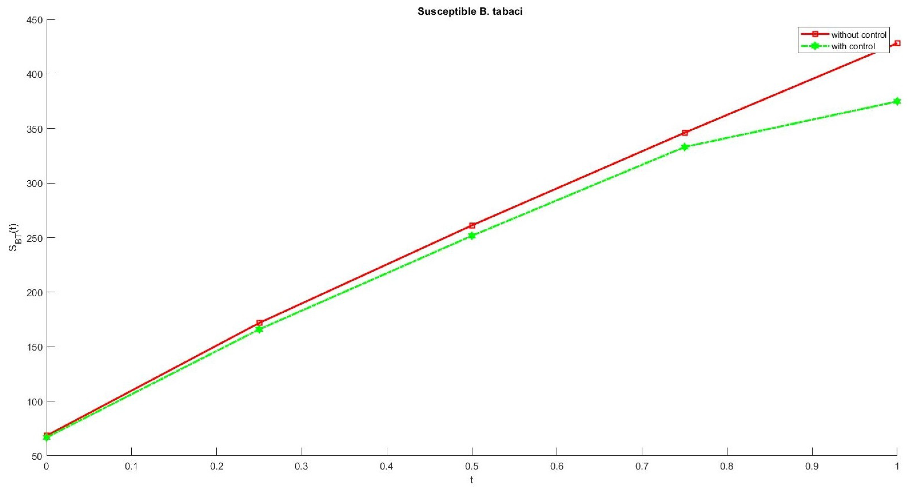
6. Numerical Results

Here, we examine the mathematical model of C. annuum with AB fractional derivative and optimal control numerically. We assume initial conditions and parameter values in

Table 1. Parametric representation with approximation values of (1) in [29].

Variable with Values	Definition
$N_p=80$	C. annuum population
$N_v=40$	B. tabaci population
$S_v=50$	Vegetative phase of Susceptible C. annuum
$I_v=10$	Vegetative phase of Infected C. annuum
$S_g=30$	Generative phase of Susceptible C. annuum
$I_g=10$	Generative phase of Infected C. annuum
$S_{BT}=30$	B. tabaci Susceptible insect
$I_{BT}=10$	B. tabaci Infected insect
$A=10$	Recruitment of C. annuum
$B=10$	Recruitment of B. tabaci
$\alpha =0.07$	Rate of growth from vegetative to generative phase
${\beta }_1=0.001$	Rate of infected C. annuum in the vegetaive phase
${\beta }_2=0.001$	Rate of infected C. annuum in the generative phase
${\gamma }_1=0.025$	Rate of B. tabaci infection in the vegetaive phase
${\gamma }_2=0.02$	Rate of B. tabaci infection in the generative phase
${\delta }_p=0.2$	V. lecanii
${\mu }_p=0.03$	The death rate of C. annuum
${\mu }_1=0.07$	Rate of natural death in B. tabaci
${\theta }_1=0.05$	The death rate of B. tabaci due to curative intervention

with $\zeta =0.9$ and $N\left(\zeta \right)=1$.

The optimal control is

$$\begin{array}{cc}\hfill u_1^{*}& =max\{min[\frac{1}{2A}({\lambda }_1^{*}{\beta }_1{S}_v{I}_{BT}-{\lambda }_2^{*}{\beta }_1{S}_v{I}_{BT}+{\lambda }_3^{*}{\beta }_2{S}_g{I}_{BT}-{\lambda }_4^{*}{\beta }_2{S}_g{I}_{BT}\hfill \\ & +{\lambda }_5^{*}{\gamma }_1{I}_v{S}_{BT}+{\lambda }_5^{*}{\gamma }_2{I}_g{S}_{BT}-{\lambda }_5^{*}{\theta }_1{S}_{BT}{N}_p-{\lambda }_6^{*}{\gamma }_1{I}_v{S}_{BT}-{\lambda }_6^{*}{\gamma }_2{I}_g{S}_{BT}-{\lambda }_6^{*}{\theta }_1{I}_{BT}{N}_p),1],0\}\hfill \end{array}$$

since $0\le u_1\le 1$. Consider $u_1=0.6$ and using the parametric values in (7) then,

$$\begin{array}{cc}\hfill S_{nv}\left(t\right)& =50+\left(0.1+\frac{{\left(t\right)}^{0.9}}{\mathsf{\Gamma }\left(0.9\right)}\right)[10-0.07S_{(n-1)v}\left(t\right)-0.001\times 0.4\times S_{(n-1)v}\left(t\right)I_{(n-1)BT}\left(t\right)\hfill \\ & -0.03S_{(n-1)v}\left(t\right)]\hfill \\ \hfill I_v\left(t\right)& =10+\left(0.1+\frac{{\left(t\right)}^{0.9}}{\mathsf{\Gamma }\left(0.9\right)}\right)[0.001\times 0.4\times S_{(n-1)v}\left(t\right)I_{(n-1)BT}\left(t\right)-0.03I_{(n-1)v}\left(t\right)]\hfill \\ \hfill S_g\left(t\right)& =30+\left(0.1+\frac{{\left(t\right)}^{0.9}}{\mathsf{\Gamma }\left(0.9\right)}\right)[0.07S_{(n-1)v}\left(t\right)-0.001\times 0.4\times S_{(n-1)g}\left(t\right)I_{(n-1)BT}\left(t\right)\hfill \\ & -0.03S_{(n-1)g}\left(t\right)]\hfill \\ \hfill I_g\left(t\right)& =10+\left(0.1+\frac{{\left(t\right)}^{0.9}}{\mathsf{\Gamma }\left(0.9\right)}\right)[0.001\times 0.4\times S_{(n-1)g}\left(t\right)I_{(n-1)BT}\left(t\right)-0.03I_{(n-1)g}\left(t\right)]\hfill \\ \hfill S_{BT}\left(t\right)& =30+\left(0.1+\frac{{\left(t\right)}^{0.9}}{\mathsf{\Gamma }\left(0.9\right)}\right)[10\times 40-0.025\times 0.4\times I_{(n-1)v}\left(t\right)S_{(n-1)BT}\left(t\right)-0.02\hfill \\ & \times 0.4\times I_{(n-1)g}\left(t\right)S_{(n-1)BT}\left(t\right)-0.05\times 0.6\times S_{(n-1)BT}\left(t\right)\times 80-0.07S_{(n-1)BT}\left(t\right)]\hfill \\ \hfill I_{BT}\left(t\right)& =10+\left(0.1+\frac{{\left(t\right)}^{0.9}}{\mathsf{\Gamma }\left(0.9\right)}\right)[0.025\times 0.4\times I_{(n-1)v}\left(t\right)S_{(n-1)BT}\left(t\right)+0.02\times 0.4\hfill \\ & \times I_{(n-1)g}\left(t\right)S_{(n-1)BT}\left(t\right)-0.05\times 0.6\times I_{(n-1)BT}\left(t\right)\times 80-0.07I_{(n-1)BT}\left(t\right)]\hfill \end{array}$$

which gives the numerical values plotted in Figure 1, Figure 2, Figure 3, Figure 4, Figure 5 and Figure 6.

In Figure 1, Figure 2, Figure 3, Figure 4, Figure 5 and Figure 6, we show that the use of 60% V. lecanni for 5 days changed the population of susceptible and infected plants in vegetative and generative phases, as well as the variation of population of susceptible and infected white bugs.

When $u_1=0$, i.e., without V. lecanni, the control system reduce to the model given below:

$$\begin{array}{cc}\hfill {}_0^{ABC}{D}_t^{\zeta }{S}_v\left(t\right)& =A-\alpha S_v-{\beta }_1{S}_v{I}_{BT}-{\mu }_p{S}_v\hfill \\ \hfill {}_0^{ABC}{D}_t^{\zeta }{I}_v\left(t\right)& ={\beta }_1{S}_v{I}_{BT}-{\mu }_p{I}_v\hfill \\ \hfill {}_0^{ABC}{D}_t^{\zeta }{S}_g\left(t\right)& =\alpha S_v-{\beta }_2{S}_g{I}_{BT}-{\mu }_p{S}_g\hfill \\ \hfill {}_0^{ABC}{D}_t^{\zeta }{I}_g\left(t\right)& ={\beta }_2{S}_g{I}_{BT}-{\mu }_p{I}_g\hfill \\ \hfill {}_0^{ABC}{D}_t^{\zeta }{S}_{BT}\left(t\right)& =B{N}_v-{\gamma }_1{I}_v{S}_{BT}-{\gamma }_2{I}_g{S}_{BT}-{\mu }_1{S}_{BT}\hfill \\ \hfill {}_0^{ABC}{D}_t^{\zeta }{I}_{BT}\left(t\right)& ={\gamma }_1{I}_v{S}_{BT}+{\gamma }_2{I}_g{S}_{BT}-{\mu }_1{I}_{BT}.\hfill \end{array}$$

In Figure 7, Figure 8, Figure 9, Figure 10, Figure 11 and Figure 12, we compare the numerical values of the variables $S_v\left(t\right)$, $I_v\left(t\right)$, $S_g\left(t\right)$, $I_g\left(t\right)$, $S_{BT}\left(t\right)$ and $I_{BT}\left(t\right)$ with and without V. lecanii $u_1$. The comparison of these variables of ordinary differential equations is shown in [29] of the figures are Figure 2, Figure 3, Figure 4, Figure 5, Figure 6 and Figure 7. The results with V. lecanni in each stage of plants and insects are more effective and accurate in Atangana–Baleanu fractional derivative than ordinary differential equations stated in [29].

Figure 7 and Figure 9 show that the susceptible C. annuum in vegetative and generative phases, which increased the population by 1% with V. lecanni compared to that of without V. lecanni because the infected B. tabaci cannot transmit the virus through chili plants. Figure 8 and Figure 10 show the comparison of infected C. annuum in vegetative and generative phases, which decrease the population by 1% with V. lecanni compared to that of without V. lecanni.

In Figure 11, the comparison of susceptible B. tabaci population decreases with V. lecanni by 50% compared to that of without V. lecanni because the infected B. tabaci cannot infect the healthy one with an antidote. In Figure 11, the comparison of infected B. tabaci population decreases with V. lecanni by 4% compared to that of without V. lecanni because the infected ones were either cured or dead due to curative intervention.

In Figure 13, the measure of implementing 60% of V. lecanni per day will reduce 1% of infected C. annuum and 1% of infected B. tabaci. By continuing this process, the 60% of V. lecanni control the spread of the yellow virus within 10 days, which helps the farmers to afford the costs of cultivating the C. annuum.

7. Conclusions

In this study, we described the C. annuum model of the yellow virus in two discrete aspects. First, we examined the C. annuum model and applied the optimal control. Second, we analyzed the C. annuum model using the Atangana–Baleanu derivative. The threshold quantity is less than one when the presented model is locally stable. Furthermore, the model is globally stable when ${\psi }_0>1$. With the help of V. lecanii (an entomopathogenic fungus), $u_1\left(t\right)$ optimal control reduced the population of infected B. tabaci and C. annuum. The numerical results of optimal conditions of the C. annuum model with AB-derivative are described detailly by successive approximation method. The infected population of C. annuum increases and decreases according to V. lecanii use and vice-versa for susceptible. The results show that using 60% of V. lecanni controls the spread of the yellow virus in infected B. tabaci and C. annuum over 10 days, which helps farmers to afford the costs of cultivation.

References

1. Mariyono, J. Impacts seed technology improvement on economic aspects of chilli production in central java-Indonesia. J. Ekon. Pembang. 2016, 17, 1–14. [Google Scholar] [CrossRef] [Green Version]
2. Khan, F.A.; Mahmood, T.; Ali, M.; Saeed, A.; Maalik, A. Pharmacological importance of an ethnobotanical plant: Capsicum annuum L. Nat. Prod. Res. 2014, 28, 1267–1274. [Google Scholar] [CrossRef] [PubMed]
3. Subban, R.; Sundaram, K. Effect of Antiviral Formulations on Chilli Leaf Curl Virus (CLCV) Disease of Chilli Plant (Capsicum annuum L.). J. Pharm. Res. 2012, 5, 5363–5366. [Google Scholar]
4. Solahudin, M.; Pramudya, B.; Manaf, R. Gemini Virus Attack Analysis in Field of Chili (Capsicum annuum L.) Using Aerial Photography and Bayesian Segmentation Method. Procedia Environ. Sci. 2015, 24, 254–257. [Google Scholar] [CrossRef] [Green Version]
5. Ganefianti, D.W.; Hidayat, H.S.; Syukur, M. Susceptible Phase of Chili Pepper Due to Yellow Leaf Curl Begomovirus Infection. Int. J. Adv. Sci. Eng. Inf. Technol. 2017, 7, 594–601. [Google Scholar] [CrossRef]
6. Bouhous, M.; Larous, L. Efficiency of the entomopathogenic fungus Verticillium lecanii in the biological control of Trialeurodes vaporariorum, (Homoptera: Aleyrodidae), a greenhouse culture pest. Afr. J. Microbiol. Res. 2012, 6, 2435–2442. [Google Scholar]
7. Alavo, T.B.C. The insect pathogenic fungus Verticillium lecanii (Zimm.) Viegas and its use for pests control: A review. J. Exp. Biol. Agric. Sci. 2015, 3, 337–345. [Google Scholar]
8. Sopp, P.I.; Gillespie, A.T.; Palmer, A. Application of Verticillium lecanii for the control of Aphis gossypii by a low-volume electrostatic rotary atomiser and a high-volume hydraulic sprayer. Entomophaga 1989, 34, 417–428. [Google Scholar] [CrossRef]
9. Podlubny, I. Fractional Differential Equations: An Introduction to Fractional Derivatives, Fractional Differential Equations, to Methods of Their Solution and Some of Their Applications; Academic Press: San Diego, CA, USA, 1999. [Google Scholar]
10. Ross, B. A brief history and exposition of the fundamental theory of fractional calculus. Fract. Calc. Appl. 2006, 457, 1–36. [Google Scholar]
11. Caputo, M.; Fabrizio, M. On the notion of fractional derivative and applications to the hysteresis phenomena. Meccanica 2017, 52, 3043–3052. [Google Scholar] [CrossRef]
12. Atangana, A.; Hammouch, Z. Fractional calculus with power law: The cradle of our ancestors. Eur. Phys. J. Plus 2019, 134, 429. [Google Scholar] [CrossRef]
13. Arqub, O.A.; Al-Smadi, M. Numerical solutions of Riesz fractional diffusion and advection-dispersion equations in porous media using iterative reproducing kernel algorithm. J. Porous Media 2020, 23, 783–804. [Google Scholar] [CrossRef]
14. Arqub, O.A.; Shawagfeh, N. Application of reproducing kernel algorithm for solving Dirichlet time-fractional diffusion-Gordon types equations in porous media. J. Porous Media 2019, 22, 411–434. [Google Scholar] [CrossRef]
15. Arqub, O.A. Application of residual power series method for the solution of time-fractional Schrodinger equations in one-dimensional space. Fundam. Informaticae 2019, 166, 87–110. [Google Scholar] [CrossRef]
16. Djennadi, S.; Shawagfeh, N.; Arqub, O.A. A fractional Tikhonov regularization method for an inverse backward and source problems in the time-space fractional diffusion equations. Chaos Solitons Fractals 2021, 150, 111127. [Google Scholar] [CrossRef]
17. Atangana, A.; Baleanu, D. New fractional derivatives with non-local and non-singular kernel: Theory and application to heat transfer model. Therm. Sci. 2016, 20, 763–769. [Google Scholar] [CrossRef] [Green Version]
18. Jarad, F.; Abdeljawad, T.; Hammouch, Z. On a class of ordinary differential equations in the frame of Atangana–Baleanu derivative. Chaos Solitons Fractals 2018, 117, 16–20. [Google Scholar] [CrossRef]
19. Ravichandran, C.; Logeswari, K.; Jarad, F. New results on existence in the framework of Atangana–Baleanu derivative for fractional integro-differential equations. Chaos Solitons Fractals 2019, 125, 194–200. [Google Scholar] [CrossRef]
20. Logeswari, K.; Ravichandran, C. A new exploration on existence of fractional neutral integro-differential equations in the concept of Atangana–Baleanu derivative. Physica A 2020, 544, 123454. [Google Scholar] [CrossRef]
21. Ravichandran, C.; Logeswari, K.; Panda, S.K.; Nisar, K.S. On new approach of fractional derivative by Mittag–Leffler kernel to neutral integro-differential systems with impulsive conditions. Chaos Solitons Fractals 2020, 139, 110012. [Google Scholar] [CrossRef]
22. Bonyah, E.; Gómez-Aguilar, J.F.; Adu, A. Stability analysis and optimal control of a fractional human African trypanosomiasis model. Chaos Solitons Fractals 2018, 117, 150–160. [Google Scholar] [CrossRef]
23. Alzahrani, E.O.; Khan, M.A. Modeling the dynamics of Hepatitis E with optimal control. Chaos Solitons Fractals 2018, 116, 287–301. [Google Scholar] [CrossRef]
24. Logeswari, K.; Ravichandran, C.; Nisar, K.S. Mathematical model for spreading of COVID-19 virus with the Mittag–Leffler kernel. Numer. Methods Partial. Differ. Equ. 2020, 1–16. [Google Scholar] [CrossRef] [PubMed]
25. Tassaddiq, A.; Khan, I.; Nisar, K.S. Heat transfer analysis in sodium alginate based nanofluid using MoS2 nanoparticles: Atangana–Baleanu fractional model. Chaos Solitons Fractals 2020, 130, 109445. [Google Scholar] [CrossRef]
26. Korpinar, Z.; Inc, M.; Bayram, M. Theory and application for the system of fractional Burger equations with Mittag leffler kernel. Appl. Math. Comput. 2020, 367, 124781. [Google Scholar] [CrossRef]
27. Panda, S.K.; Ravichandran, C.; Hazarika, B. Results on system of Atangana–Baleanu fractional order Willis aneurysm and nonlinear singularly perturbed boundary value problems. Chaos Solitons Fractals 2021, 142, 110390. [Google Scholar] [CrossRef]
28. Sweilam, N.H.; Al-Mekhlafi, S.M.; Assiri, T.; Atangana, A. Optimal control for cancer treatment mathematical model using Atangana–Baleanu-Caputo fractional derivative. Adv. Differ. Equ. 2020, 2020, 334. [Google Scholar] [CrossRef]
29. Amelia, R.; Anggriani, N.; Supriatna, A.K. Optimal Control Model of Verticillium lecanii Application in the Spread of Yellow Red Chili Virus. WSEAS Trans. Math. 2019, 18, 351–358. [Google Scholar]
30. Sweilam, N.H.; L-Mekhlafi, S.M.A. On the optimal control for fractional multi-strain TB model. Optim. Control Appl. Methods 2016, 37, 1355–1374. [Google Scholar] [CrossRef]
31. Trigeassou, J.-C.; Maamri, N. Optimal State Control of Fractional Order Differential Systems: The Infinite State Approach. Fractal Fract. 2021, 5, 29. [Google Scholar] [CrossRef]
32. Wang, F.; Li, X.; Zhou, Z. Spectral Galerkin Approximation of Space Fractional Optimal Control Problem with Integral State Constraint. Fractal Fract. 2021, 5, 102. [Google Scholar] [CrossRef]
33. Caputo, M.; Fabrizio, M. A new Definition of Fractional Derivative without Singular Kernel. Prog. Fract. Differ. Appl. 2015, 1, 73–85. [Google Scholar]
34. Brauer, F.; den Driessche, P.V.; Wu, J. Mathematical Epidemiology; Springer: Berlin/Heidelberg, Germany, 2008. [Google Scholar]
35. Agrawal, O.P. On a general formulation for the numerical solution of optimal control problems. Int. J. Control 1989, 50, 627–638. [Google Scholar] [CrossRef]
36. Agrawal, O.P. Formulation of Euler-Lagrange equations for fractional variational problems. J. Math. Anal. Appl. 2002, 272, 368–379. [Google Scholar] [CrossRef] [Green Version]
37. Agrawal, O.P. A formulation and numerical scheme for fractional optimal control problems. IFAC Proc. Vol. 2006, 39, 68–72. [Google Scholar] [CrossRef]
38. Agrawal, O.P.; Defterli, O.; Baleanu, D. Fractional optimal control problems with several state and control variables. J. Vib. Control 2010, 16, 1967–1976. [Google Scholar] [CrossRef]
Figure 1. Optimal control of susceptible vegetative phase S v ( t ) of C. annuum.
Fractalfract 06 00061 g001
Figure 2. Optimal control of infected vegetative phase I v ( t ) of C. annuum.
Fractalfract 06 00061 g002
Figure 3. Optimal control of susceptible generative phase S g ( t ) of C. annuum.
Fractalfract 06 00061 g003
Figure 4. Optimal control of infected generative phase I v ( g ) of C. annuum.
Fractalfract 06 00061 g004
Figure 5. Optimal control of susceptible B. tabaci S B T ( t ) in C. annuum.
Fractalfract 06 00061 g005
Figure 6. Optimal control of infected B. tabaci I B T ( t ) in C. annuum.
Fractalfract 06 00061 g006
Figure 7. Comparison of susceptible vegetative phase S v ( t ) in C. annuum with and without V. lecanni.
Fractalfract 06 00061 g007
Figure 8. Comparison of infected vegetative phase I v ( t ) in C. annuum with and without V. lecanni.
Fractalfract 06 00061 g008
Figure 9. Comparison of susceptible generative phase S g ( t ) in C. annuum with and without V. lecanni.
Fractalfract 06 00061 g009
Figure 10. Comparison of infected generative phase I v ( g ) in C. annuum with and without V. lecanni.
Fractalfract 06 00061 g010
Figure 11. Comparison of susceptible B. tabaci S B T ( t ) in C. annuum with and without V. lecanni.
Fractalfract 06 00061 g011
Figure 12. Comparison of infected B. tabaci I B T ( t ) in C. annuum with and without V. lecanni.
Fractalfract 06 00061 g012
Figure 13. Control of V. lecanni.
Fractalfract 06 00061 g013