1. Introduction
The importance of nanofluids has been growing with the passage of time, and investigators have been intending to examine the attitude of nanofluids subjected to heat transport systems. Nanofluids and their inclusions in the industrial sector have been growing more due to their homogeneous nature in thermal conductivity and rudimentary heat transport. Regular fluids such as water, propylene glycol, and ethylene glycol, among others, have poor heat transport properties. Nanoliquids, a homogenous solid liquid mixture, are applied to promote the classical, heat transfer base fluids thermal conductivity. Nanofluids have a vast domain of applications, including cancer therapy, microelectronics cooling, imaging, sensing, vehicle and industrial cooling, the evolution of new kinds of cooling towers, fuels, cooling and heating of household appliances, and hybrid-powered engine efficiency, etc. [
1,
2,
3]. Choi [
4] coined the term nanoparticle to characterize a particle that improves the thermal conductivity of nanoparticles. In order to realize how thermal conductivity is improved, he provided many numerical and experimental studies. Khanafer et al. [
5] examined the impact of nanomaterials on convection exploring that driving nanomaterials at some Grashof number considered a rapid thermal conductivity. Sun et al. [
6] studied the influence of nanomaterial size and considered this improving nanoparticle size improves heat capacity.
Meanwhile, magnetohydrodynamics (MHD) also has a pivotal role in the effective application of fluid flow and heat transport. MHD is widely applied to investigate the properties of magnetic fields and the conduct of electrically conducting liquids. The definition of MHD is coming from the word magnetohydrodynamics, which far boost the meaning of magnetic field, water, and movement, respectively. The basic principle underlying the MHD is that magnetic fields produce currents in a flowing conducting liquid, polarizing, in turn, the liquid and changing the magnetic field itself. The magnetic field is useful in material processes, heat exchangers, and scientific research. The magnetic field can create a force which is used in water evaporation, silver deposition, and protein crystallization, etc. However, the MHD boundary layer flows also grow in MHD power generator designs, plasma studies, liquid metal manipulation, cooling of nuclear reactors, plasma cutting, induction heating, etc. Mabood et al. [
7] addressed the magnetoflow of nanofluid and heat transfer along the stretching sheet. Srinivasacharya et al. [
8] analyzed magnetic nanofluid flow across a wedge. The problem of magnetized nanofluid flow over a stretchable surface was analyzed by Rashed et al. [
9]. Yohannes and Shanker [
10] analyzed melting heat transfer in magnetonanofluid flow over a porous sheet. Free convection flow of magnetic nanofluid through a vertical semi-infinite flat plate was discussed by Hamad et al. [
11]. Rajesh and Chamkha [
12] studied and analyzed the heat transport and free convective flowing of nanofluid through an orthogonal plate under magnetic field influence. Nabwey et al. [
13] analyzed the unsteady flow of ferrofluid along the radiative stretchable surface with convective heating. Khan et al. [
14] investigated the impact of heat generation on magnetonanofluid free convection flow about sphere in the plume region.
Industrial and physiological evolutions and the non-Newtonian materials flow are more known than the viscous fluids. The kind involves the assortment of non-Newtonian materials. Essentially, there is no integrated constitutive rheological relevance that can classify all non-Newtonian material topics to their various, assigning fields such as shear thinning, viscoelasticity, shear thickening and viscoplasticity, among others. Thus, many constitutive rheological non-Newtonian material patterns were encouraged. Among those, the micropolar liquid pattern is one that appoints the water solutions showing a great level of polymer concentration. Lately, many investigators have been focused on the prominent characteristics of micropolar liquid flows subject to diverse geometries. The first to present the micropolar fluid theory was Eringen [
14,
15]. Airman [
16,
17] introduced many types of research on micropolar fluids implementations. Bourantas and Loukopoulos [
18] formulated the free convective flow of micropolar nanoliquids. They examined that the microrotations in general reduce overall heat transport from the heated side and thus should not be removed. Rashad et al. [
19] investigated the flow of a micropolar nanoliquid along a circular cylinder in a porous medium employing convective boundary conditions. They noted that the skin friction and heat transference depend on the volume fraction of nanoparticles and material parameters. Rashad et al. [
20] also studied the unsteady slip flow of a polar nano liquid over a vertical moving surface. They concluded that the skin friction declines expressively along the moving surface for both metallic and nonmetallic nanoparticles. Other recent investigations reported by authors relevant to this topic could be found in references [
21,
22].
This study explores the magneto-free convective of micropolar nanofluid flow through a solid sphere, considering the Newtonian heating. The goal of the evaluations is to diagnose the effects of various governing parameters on velocity, temperature, angular velocity curves, and the variations of skin friction and Nusselt number along different positions. This simulation is pertinent to multiphysical magnetic micropolar nanoliquid materials processing.
2. Basic Equations
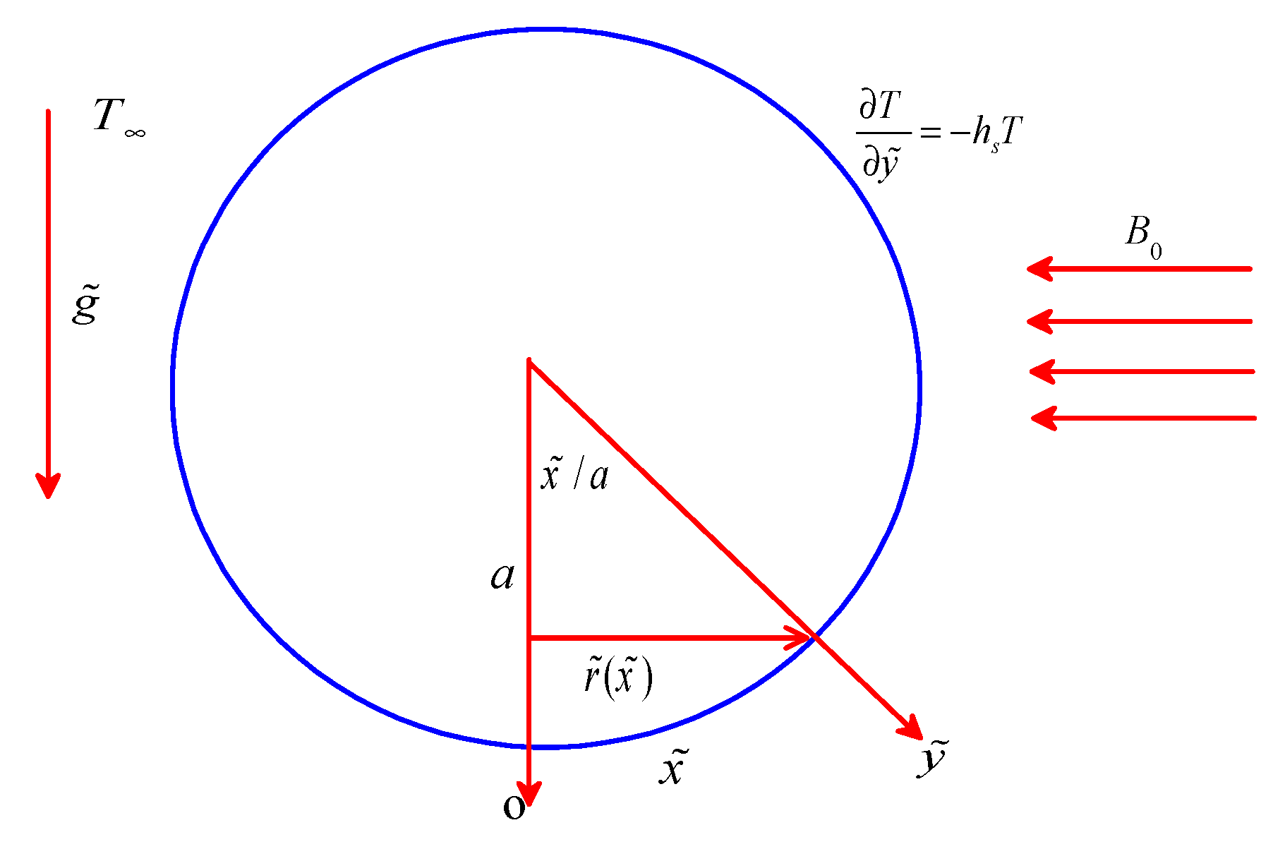
Consider the steady laminar 2-D incompressible magneto-free convective flow of copper (Cu) and cobalt (Co) water-based micropolar nanofluid over a heated sphere of the radius
a which is immersed in a viscous and incompressible micropolar fluid of ambient temperature
and subjected to a Newtonian heating(NH) as shown in
Figure 1, where
is the gravity vector, the
coordinate is measured along the surface of the solid sphere at the lower stagnation point (
), the
coordinate is measured the distance normal to the surface of the sphere, and
is the radial distance from the symmetricalaxis to the surface of the solid sphere. A uniform magnetic field
B0 is utilized in the direction perpendicular to the surface. Under the Boussinesq and boundary layer approximations, the basic equations are (Salleh et al. [
23]);
The boundary conditions of Equations (1)–(4) are:
where (
) stand for the velocity components along
axes.
is the angular velocity,
is the temperature of the fluid,
is the acceleration,
is the microinertia density,
is the vortex viscosity,
is the magnetic field strength, and
is the heat transfer coefficient for Newtonian heatingcondition.
The nondimensional variables are defined as ([
23]):
Substituting Equation (6) into Equations (1)–(4) as follows:
The boundary condition for Equations (7)–(10) are defined as:
where
,
,
,
are the micropolar parameter, magnetic parameter, Prandtl number, and Grashof number, respectively.
is the conjugate parameter for Newtonian heating case (NH). From condition (11),
when
, corresponding to the presence of
, and thus, there is no heat from the sphere [
24]. The following variables are used to solve Equations (7)–(10) and condition (11):
where
is a stream function and defined as:
In the current research, the following thermophysical relations are applied; see Tiwari and Das’s model [
23];
where
is the thermal diffusivity,
is the spin-gradient nanofluid viscid,
is the stands for the specific heat at a uniform pressure,
is the thermal expansion coefficient of the nanofluid,
and
are the thermal expansion coefficients of the base fluid and nanoparticle, respectively, and
and
are the densities of the base fluid and nanoparticles, respectively. The dynamic viscosity for nanofluid is denoted by
, and
is the electric conductivity of the base fluid, and
is the electric conductivity of the nanoparticles.
is the effective thermal conductivity of nanofluid. The efficient thermal and physical properties of nanofluid are presented in
Table 1.
Substituting Equations (12) and (13) into Equations (7)–(10), then
with the boundary-condition:
At
(lower stagnation point) for the sphere, Equations (19)–(21) can be written as:
In addition, the boundary condition
Important quantities, namely, the skin friction coefficient
and local Nusselt number
, are defined for physical interest as follows:
Using Equations (6) and (11) thus:
At (lower stagnation point of the sphere), wall temperature and skin friction coefficient are defined as ,
3. Numerical Method
Following [
25,
26], Equations (19)–(21) with boundary conditions (22) can be solved using the local similarity and nonsimilarity methods. In the local similarity method, the first derivatives concerning
are neglected, and Equations (19)–(21) can be rewritten as:
with the same boundary conditions (22) and
Following [
25,
26], for the local nonsimilarity solution, now we hold all the terms by assuming the new auxiliary functions
and
, which are defined by
Using these functions, Equations (19)–(21) can be rewritten as
subjected to the same boundary conditions (22) and (33). The new ordinary differential Equations (34)–(37) with boundary conditions (22) represent a local nonsimilarity model. To simplify this model, these equations and the corresponding boundary conditions are now differentiated, w.r.t.
, simplified, and the derivatives, w.r.t.
, are neglected again to obtain a local similarity model and can be written as:
The ordinary differential Equations (38)–(40) with boundary conditions (22) and (33) were solved numerically by employing the Runge–Kutta–Fehlberg method (RKF45) using MAPLE software (Version 20). This software uses the most excellent method available and delivers more accurate results. The step size
and a convergence criterion of
were selected in the numerical computations. The asymptotic boundary conditions, given in Equation (22), were replaced by using a value of 10 for the similarity variable
as follows:
To ensure the proper convergence of dimensionless velocity and temperature, is selected. The value of is progressedin small intervals from the lower stagnation point to the upper stagnation point, and the derivatives of the functions are revised after every outer iteration step.
On account of the complexity of the given problem, the local similar and nonsimilar Equations (34)–(40) with boundary conditions (22) and (33) are solved by the Runge–Kutta–Fehlberg method. RKF 45th order was used with the effective choice of step h to decrease governing equations into first-order equations. Considering the function,
f (
t,
y) was applied, and the technique was written as follows;
Hence, the iterative process for the solution is obtained by using the Runge–Kutta fifth-order formula as,
As mentioned above, we chose a convenient finite value of
so that far field boundary conditions are satisfiedasymptotically. In this investigation, anappropriate finite value of
is addressed as
in such a way that not only numerical solutions converge but also boundary conditions satisfied at infinity satisfy asymptotically. The relative error tolerance to 10
−6 is addressed for convergence, and the step size is chosen as
. Moreover, the CPU time to appreciate the values of velocity profiles (1.23 s) ismuch less than the CPU time to estimate the values of temperature profiles (1.67 s), and the CPU time for angular velocity is 2.01 s. For a check, the accuracy of this numerical method was validated by comparing the present results with the results reported by Salleh et al. [
23], in the absence of magnetic field, and micropolar parameter for Newtonian pure fluid.
Table 2 presents the results of this comparison. The current results are found in an excellent agreement with the existing results.
4. Results and Discussion
The local similar and nonsimilar Equations (34)–(39) with boundary conditions (22) and (33) are solved by the Runge–Kutta–Fehlberg method. Two different Cu and Co nanoparticles are employed to investigate the effects of Newtonian heating and magnetic and micropolar parameters along the surface of a solid sphere. The present numerical results are validated with the existing results and are found in good agreement.
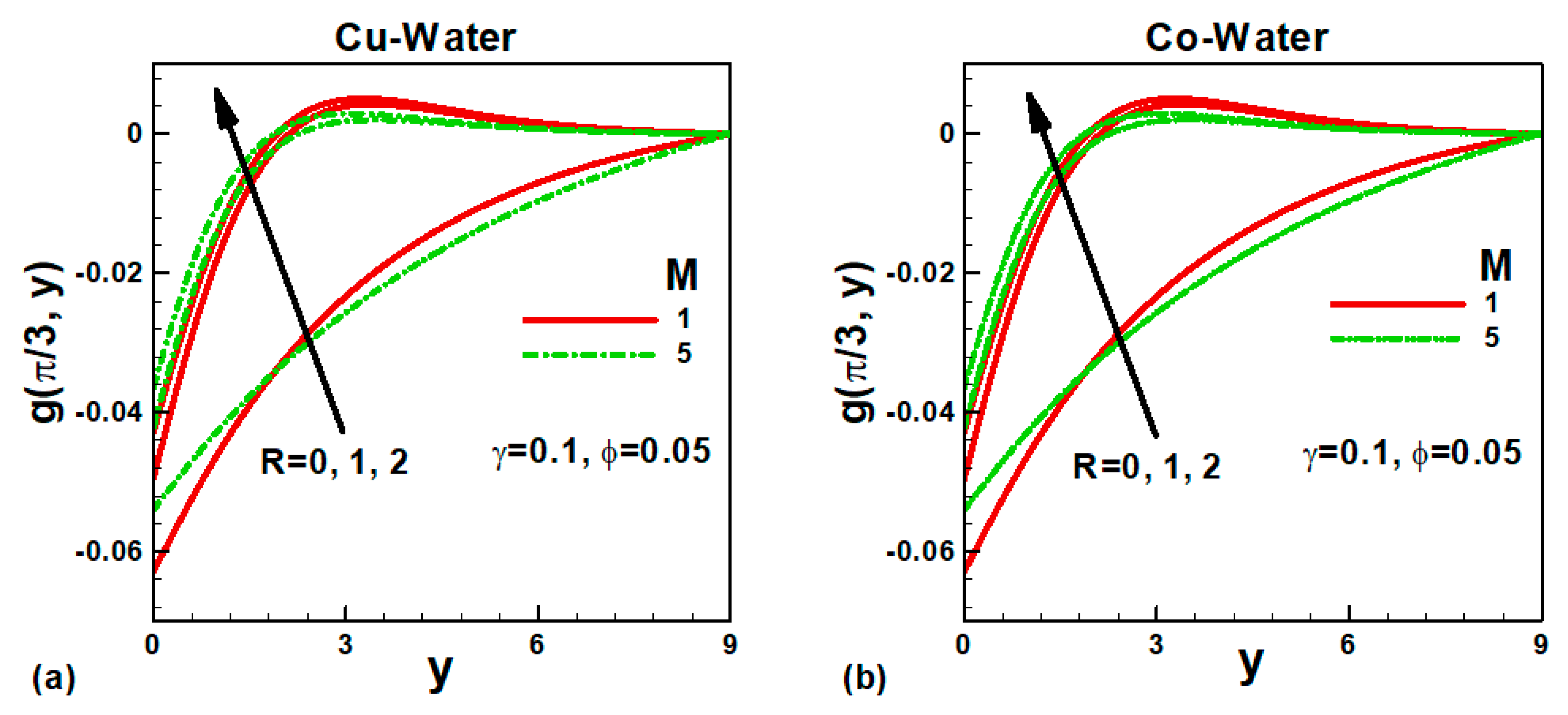
The effects of magnetic parameter M, micropolar parameter R, and solid volume fraction of both nanoparticles ϕ on velocity curves
are presented in
Figure 2 and
Figure 3 along the surface of the sphere. Due to buoyancy forces, the dimensionless velocity reaches a maximum value near the solid surface. It then goes to the ambient velocity at the edge of the velocity boundary layer. The magnetic field creates a Lorentz force, which opposes the motion of the fluid. As the magnetic field increases, the maximum velocity near the surface reduces. Consequently, the velocity boundary layer thickness increases in both cases. Physically, the encouragement of Lorentz strength through the prompting in the magnetic constraint caused a deceleration to flow and boosted the temperature for pure fluid and nanofluid at two positions. The effects of the micropolar parameter R on the dimensionless velocity are also shown in
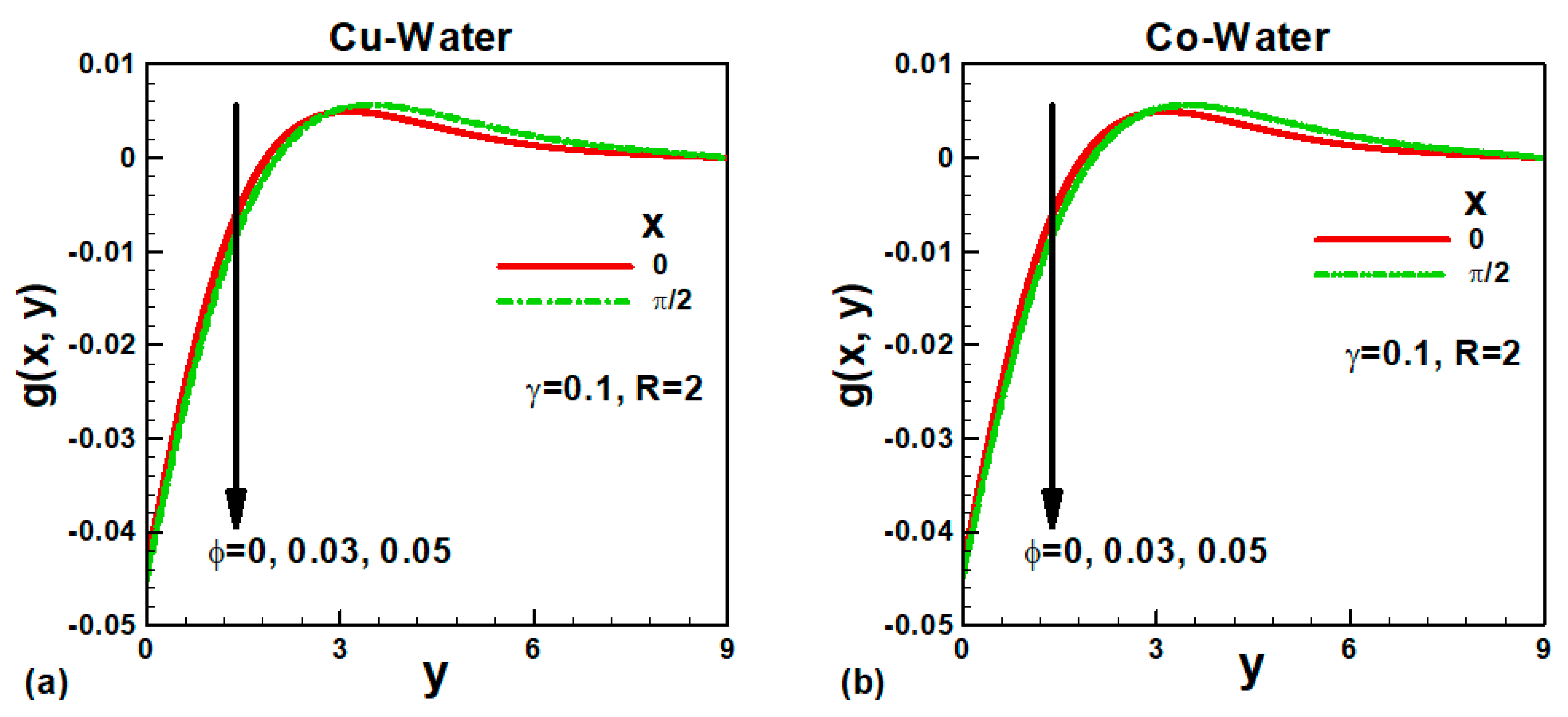
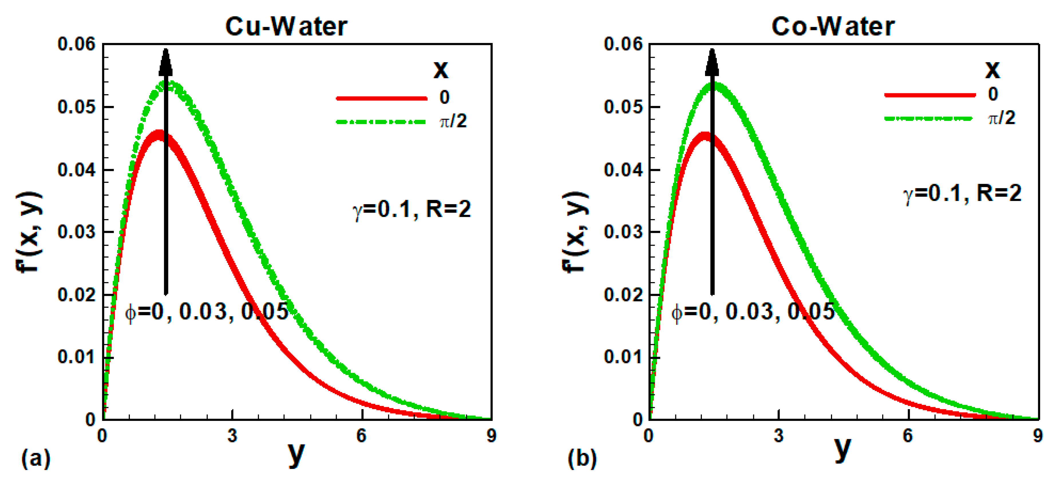
Figure 2 for both nanofluids. It is noticed that the velocity boundary layer thickness decreases as R increases from R = 0 (Newtonian fluid) to R = 2 (micropolar fluid). The variation of dimensionless velocity with a solid volume fraction of selected nanoparticles is depicted in
Figure 3a,b at the lower and upper stagnation points. The variation is examined only for micropolar fluid. The maximum velocity at the lower stagnation point is the smallest and increases along the sphere surface up to the upper stagnation point. Consequently, the velocity boundary layer thickness increases along the surface. However, no appreciable effect of solid volume fraction of nanoparticles ϕ on the dimensionless velocity could be observed.
The behavior of the dimensionless angular velocity
for different values of the magnetic parameter M is depicted in
Figure 4a,b for Newtonian and micropolar nanofluids. In this case, the solid volume fraction of both nanoparticles ϕ is taken as 5%. Due to the magnetic field’s Lorentz forces, the dimensionless angular velocity rises at the surface and within the boundary layer. For the Newtonian nanofluid (R = 0), the angular velocity is lesser at the surface and higher for the micropolar nanofluid (R = 2). The impact of solid volume fraction of selected nanoparticles ϕ on dimensionless angular velocity
is exhibited in
Figure 5a,b along the spherical surface. No noticeable effect of solid volume fraction of nanoparticles could be noticed on the angular velocity.
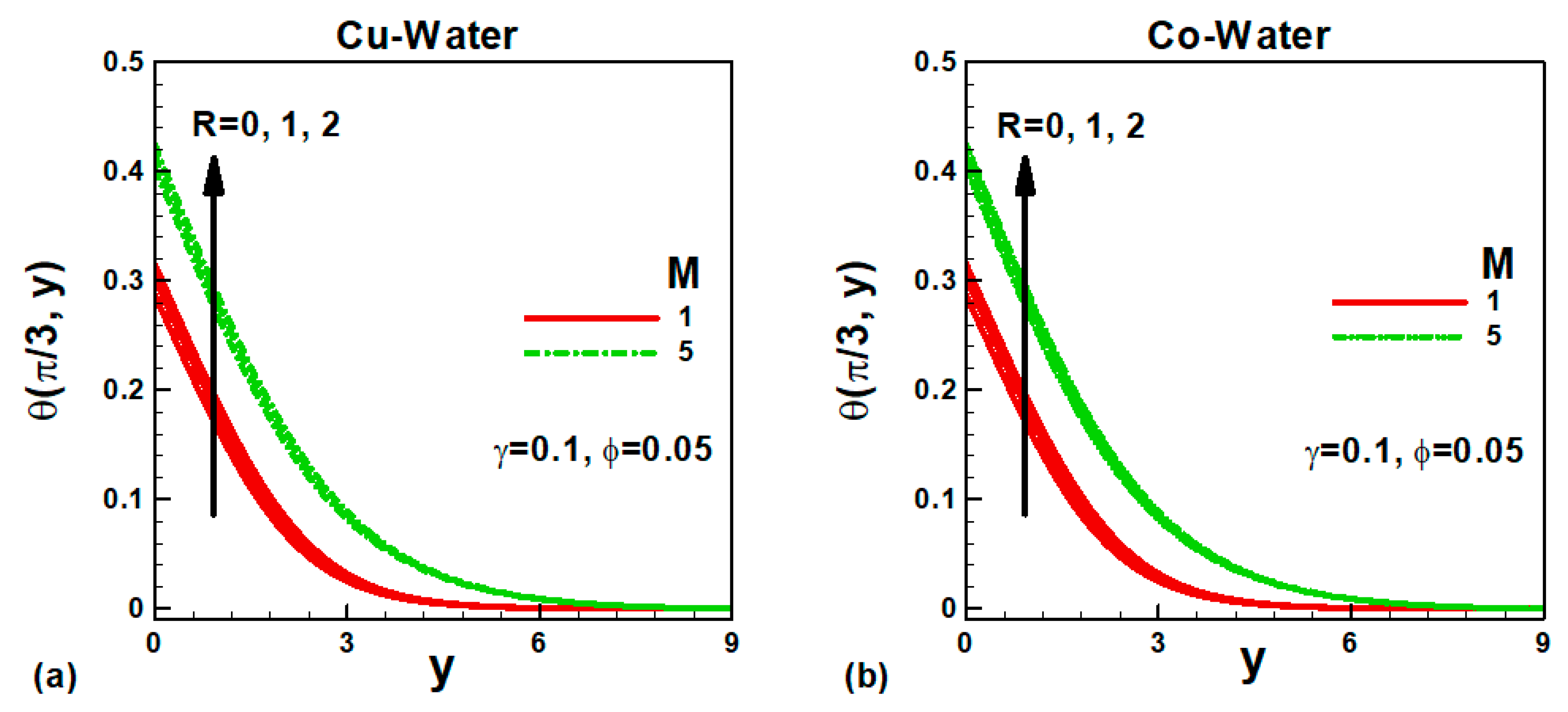
The influence of the magnetic field M on the dimensionless temperature
at the selected position is displayed in
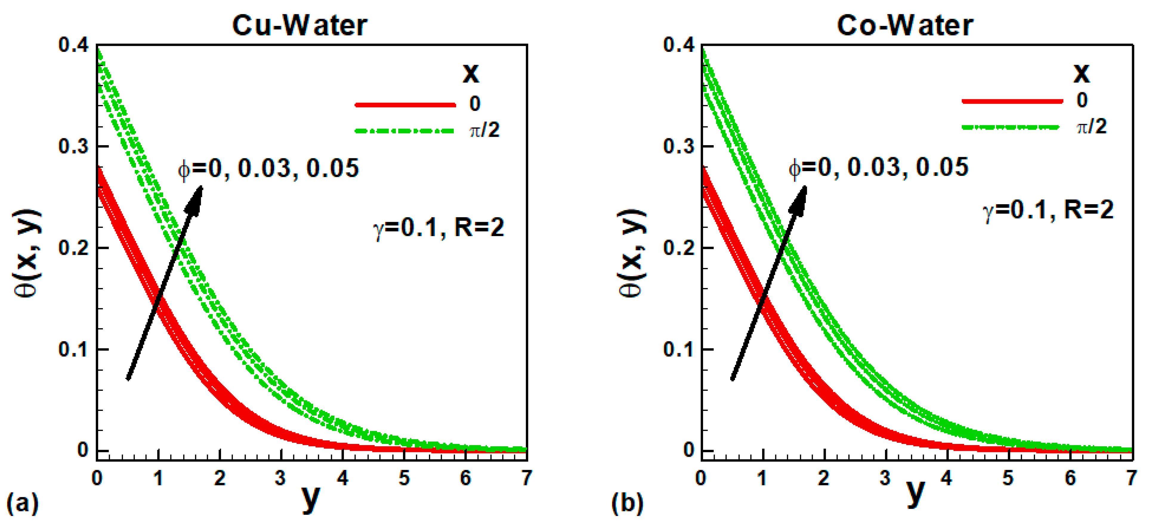
Figure 6a,b for the nanofluids under consideration. The magnetic field tends to increase the surface temperature and the boundary layer thickness in both cases. Consequently, the thermal resistance to heat flow increases with an increase in the magnetic field. For the Newtonian nanofluid, the surface temperature is found to be lower and increases for micropolar nanofluid. The variation of dimensionless temperature
with the solid volume fraction of nanoparticles ϕ is displayed in
Figure 7a,b at the lower and upper stagnation points for the micropolar fluid. The effects of the solid volume fraction of both nanoparticles are not significant. It is important to note that the dimensionless temperature increases from lower to upper stagnation points.
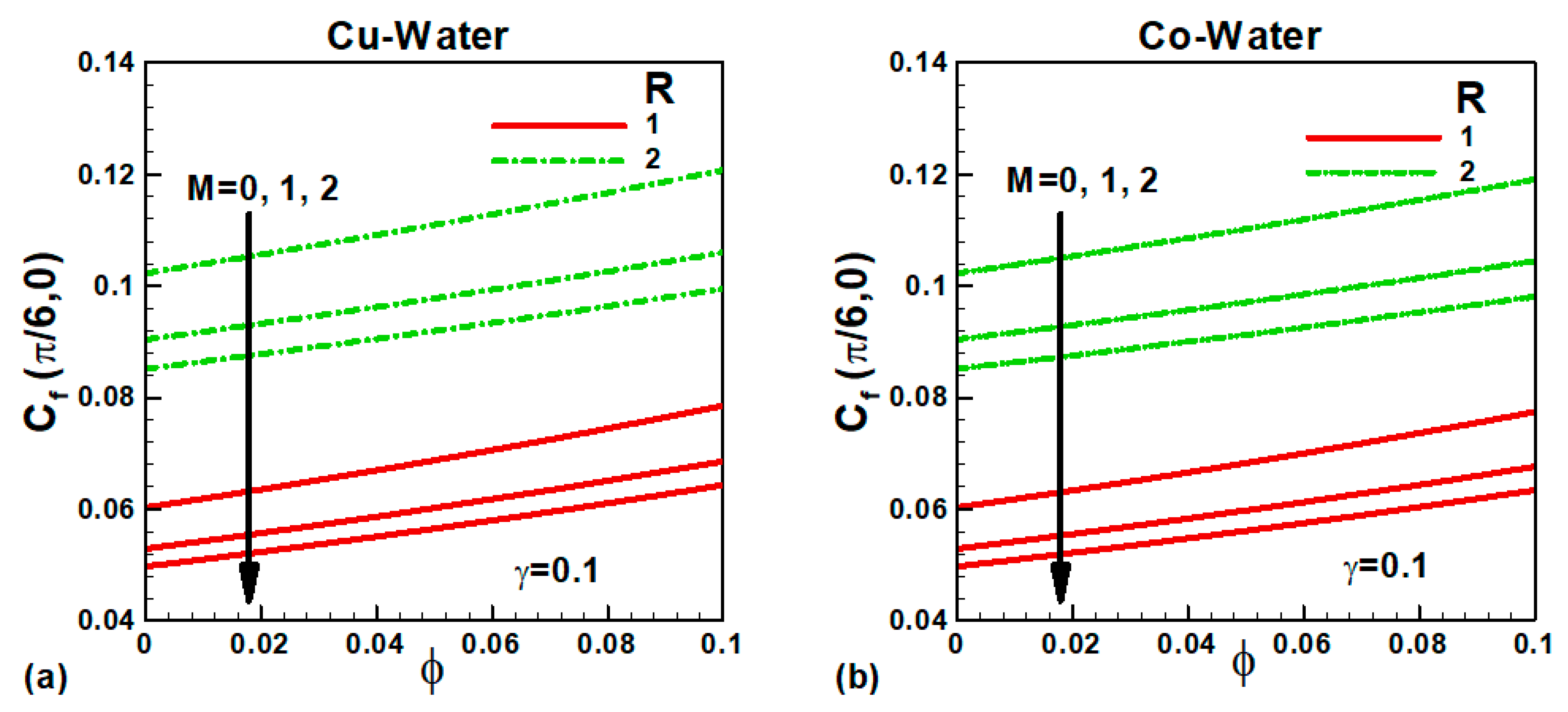
The variation of skin friction
with governing parameters is explained in
Figure 8 and
Figure 9 for both nanofluids. The variation of skin friction with the solid volume fraction of the selected nanoparticles for different magnetic field values is shown in
Figure 8a,b for micropolar nanofluids. In the absence of a magnetic field, the skin friction is higher and declines with an increase in the magnetic field due to Lorentz forces in both cases. Since both nanoparticles’ density is 9–11 times higher than water (
Table 1), the density of both nanofluids increases with an increase in the solid volume fraction of nanoparticles. As a result, the skin friction increases with φ, as shown in
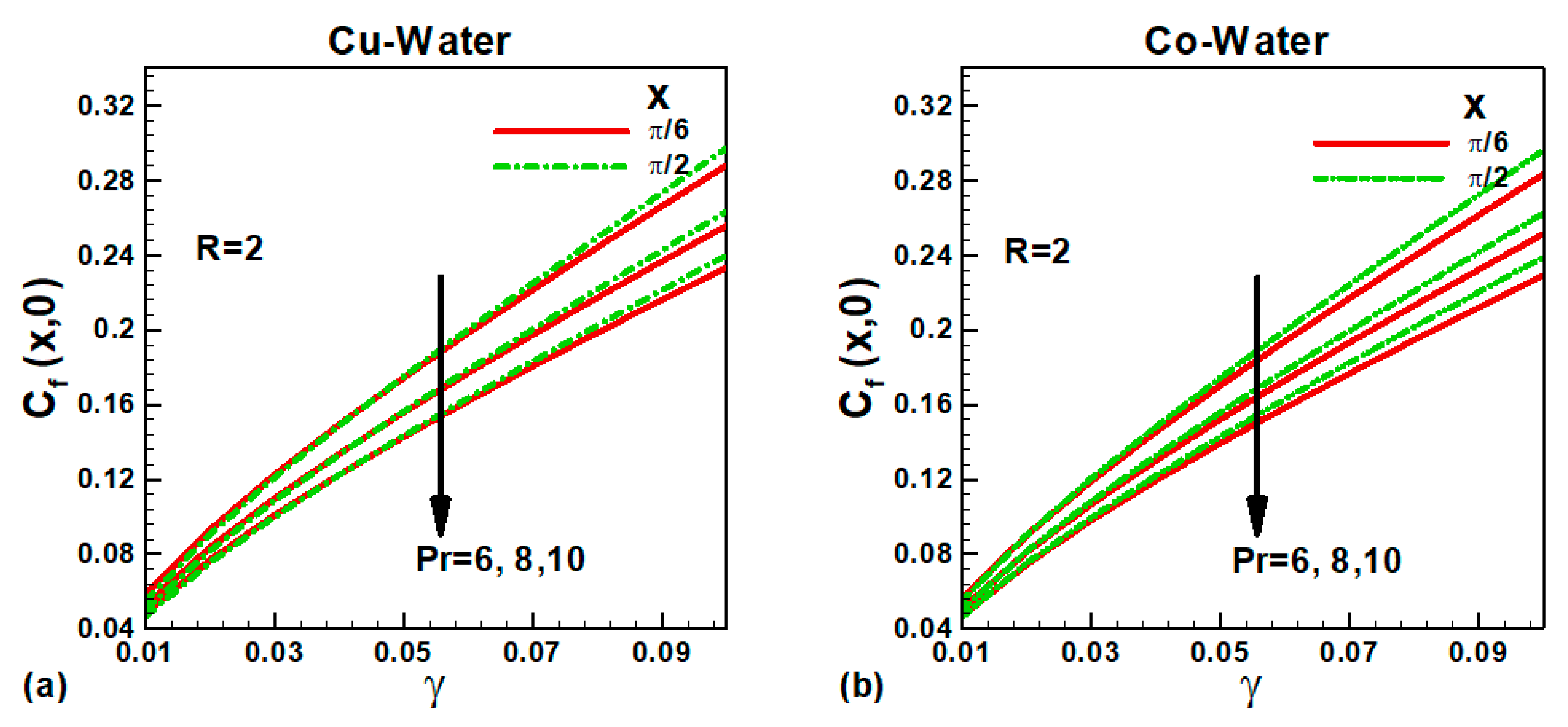
Figure 8a,b. The variation of skin friction with Newtonian heating is demonstrated in
Figure 9a,b for water-based nanofluids at different locations on the solid sphere. During Newtonian heating, surface resistance is dominant over internal resistance. Consequently, the skin friction increases with an increase in Newtonian heating and the location from lower stagnation point to upper stagnation point. The Prandtl number measures the momentum and thermal transport capacities of the fluids and varies directly with the fluid’s viscosity. Consequently, the skin friction decreases with an increase in the Prandtl number.
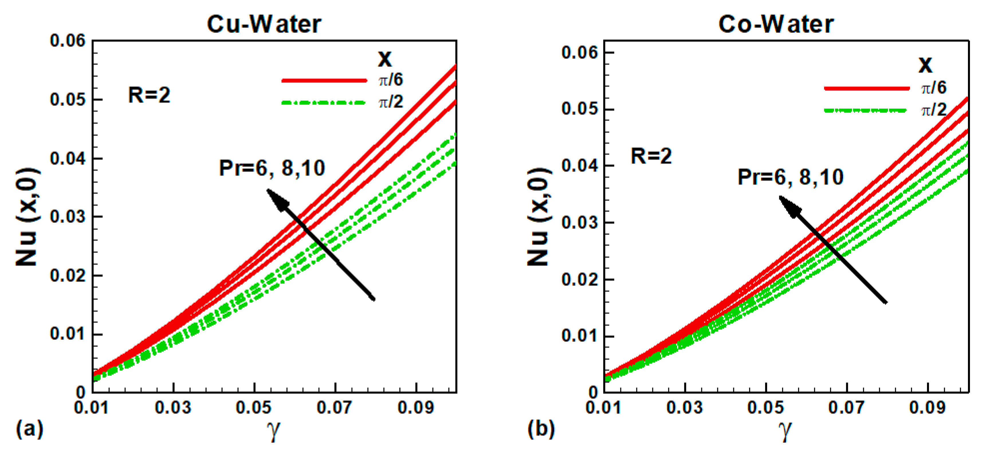
The variation of Nusselt number
with pertinent parameters is depicted in
Figure 10 and
Figure 11 for the selected nanofluids at different positions.
Figure 10a,b shows Nusselt number’s variation with the solid volume fraction of nanoparticles chosen for different magnetic parameter values. The dimensionless temperature at the surface is due to an increase in the magnetic field, which reduces the heat transfer rate. The Nusselt number varies directly with the nanofluid’s thermal conductivity, which depends upon the solid volume fraction of nanoparticles. As a result, the Nusselt number
increases with φ, as shown in
Figure 10a,b for both nanofluids at the selected position. The micropolar parameter also tends to reduce the heat transfer rate in both cases. The variation of the Nusselt number
with the Newtonian heating parameter is shown in
Figure 11a,b for different values of Prandtl number at two selected positions. It is demonstrated that the Prandtl number enhances the heat transfer rate.


