Non-Debye Relaxations: The Ups and Downs of the Stretched Exponential vs. Mittag–Leffler’s Matchings

Abstract

Experimental data collected to provide us with information on the course of dielectric relaxation phenomena are obtained according to two distinct schemes: one can measure either the time decay of depolarization current or use methods of the broadband dielectric spectroscopy. Both sets of data are usually fitted by time or frequency dependent functions which, in turn, may be analytically transformed among themselves using the Laplace transform. This leads to the question on comparability of results obtained using just mentioned experimental procedures. If we would like to do that in the time domain we have to go beyond widely accepted Kohlrausch–Williams–Watts approximation and become acquainted with description using the Mittag–Leffler functions. To convince the reader that the latter is not difficult to understand we propose to look at the problem from the point of view of objects which appear in the stochastic processes approach to relaxation. These are the characteristic exponents which are read out from the standard non-Debye frequency dependent patterns. Characteristic functions appear to be expressed in terms of elementary functions whose asymptotics is simple. This opens new possibility to compare behavior of functions used to describe non-Debye relaxations. It turnes out that the use of Mittag-Leffler function proves very convenient for such a comparison.

1. Introduction

A description of physical phenomena whose kinetics is influenced by complexity, disorder, or randomness often requires a radical departure from theoretical methods established for analogous, but simpler, phenomena discussed in textbooks of general physics. Such a situation arises when we become interested in study of dielectric relaxations and encounter their time behavior different from the commonly expected exponential decay. Depending on the experimental setup empirical investigation of the relaxation phenomena and collecting the data is done by measuring either their time behavior or frequency characteristics, i.e., the experiment provides us with data in the time or in the frequency domains. A typical example of dielectric relaxation phenomena is provided by a dipolar system which approaches the equilibrium being earlier driven out of it, i.e., polarized, by a step or alternating external electric field. Depolarization is usually described in terms of the relaxation or spectral functions [1]. The first just mentioned quantity, namely the time dependent relaxation function $n\left(t\right)$, counts dipoles surviving depolarization during the time $(0,t)\subset (0,\infty )$ and evolves form $n(0+)=1$ to $n(\infty )=0$. The frequency dependent spectral function $\hat{\varphi }\left(\mathrm{i}\omega \right)$, describing diffractive and absorptive effects, results from the analysis of phenomenological data obtained as a response of the system when it is probed by the harmonic electric field. Defined as the normalized ratio of dielectric permittivities $[\widehat{\epsilon }\left(\mathrm{i}\omega \right)-{\epsilon }_{\infty }]/[{\epsilon }_0-{\epsilon }_{\infty }]$, where ${\epsilon }_{\infty }={lim}_{\omega \to \infty }\widehat{\epsilon }\left(\mathrm{i}\omega \right)$ and ${\epsilon }_0={lim}_{\omega \to 0}\widehat{\epsilon }\left(\mathrm{i}\omega \right)$, it is complex valued function whose analytical properties stem from those obeyed by $\widehat{\epsilon }\left(\mathrm{i}\omega \right)$. Following standard rules the data obtained in the time t or in the frequency $\omega$ domains are interrelated by the Laplace transform $\mathcal{L}[-;·]$

$$\widehat{\varphi }\left(\mathrm{i}\omega \right)=1-\mathrm{i}\omega \widehat{n}\left(\mathrm{i}\omega \right),\widehat{n}\left(\mathrm{i}\omega \right)=\mathcal{L}[n\left(t\right);\mathrm{i}\omega ].$$

(1)

In typical non-Debye relaxation experiments the data measured in the time domain are usually fitted using the stretched exponential or, in physicists’ community language, the Kohlrausch–Williams–Watts (KWW) function

$$n_{KWW}\left(t\right)=exp[-{(t/\tau )}^{\alpha }]$$

(2)

with $\alpha >0$. In what follows we will consider only the case $\alpha \in (0,1)$ which preserves the interpretation of the stretched exponential as the continuous sum of Debye exponential decays weighted by a probability distribution belonging to the class of Lévy stable distributions [2,3]. Phenomenological functions usually used to fit the data in the frequency domain, called the standard non-Debye relaxation patterns, are the Cole–Cole (CC), Havriliak–Negami (HN), and Jurlewicz–Weron–Stanislawsky (JWS) models

$$\begin{array}{c}{\widehat{\varphi }}_{CC}\left(\mathrm{i}\omega \right)={[1+{\left(\mathrm{i}\omega \tau \right)}^{\alpha }]}^{-1},{\widehat{\varphi }}_{HN}\left(\mathrm{i}\omega \right)={[1+{\left(\mathrm{i}\omega \tau \right)}^{\alpha }]}^{-\beta },\mathrm{and}\hfill \\ \hfill {\widehat{\varphi }}_{JWS}\left(\mathrm{i}\omega \right)=1-{[1+{\left(\mathrm{i}\omega \tau \right)}^{-\alpha }]}^{-\beta },\end{array}$$

(3)

where $\alpha ,\beta \in (0,1]$ (The range of $\alpha$ and $\beta$ ensures that the spectral functions initially found as a fit for $\omega >0$ can be analytically continued to the upper half plane $\Im \omega >0$ and satisfy assumptions of [4] (Theorem 2.7)). Notice that the CC spectral function generalizes the Debye case ${\widehat{\varphi }}_D\left(\mathrm{i}\omega \right)={[1+\left(\mathrm{i}\omega \tau \right)]}^{-1}$ and simultaneously can be obtained from ${\widehat{\varphi }}_{HN}\left(\mathrm{i}\omega \right)$ or ${\widehat{\varphi }}_{JWS}\left(\mathrm{i}\omega \right)$ for $\beta =1$. Additionally, if we set $\alpha =1$ and $\beta \in (0,1)$ in the HN model then we get the Cole–Davidson (CD) pattern. An important property of relaxation patterns (3) is that if transformed to the time domain they all lead to the relaxation functions $n\left(t\right)$ expressed in terms of functions belonging to the family of the Mittag–Leffler functions (see Appendix A). Thus, we arrive at a two-fold way how to analyze the non-Debye relaxation phenomena-we can take into account their modelling either in terms of the KWW function or to choose the Mittag–Leffler functions. None of these approaches are singled out by fundamental theoretical arguments and thus it is understood to treat them as challengers whose usefulness is to be determined by comparison with experimental data. In our opinion, the results of such comparison lead far beyond its instructive meaning as they may be used to clarify ambiguities coming from difficulties that experiments are facing in asymptotic (short/long time and high/low frequencies) regimes. Thus, looking for arguments shedding light on choosing one of the just mentioned different approaches on experimentally observed data is worth attention and more systematic investigation.

We shall begin comparison of the Mittag–Leffler family and KWW matchings with recalling relations between the KWW and the standard Mittag–Leffler function that is responsible for the time behavior of the CC model. Although the KWW function has been used in modeling physical processes mainly in the context of relaxations (e.g., the Curie–von Schweidler law), the CC pattern is by no means restricted to this class of phenomena. Taken for real argument, $t\in {\mathbb{R}}_{+}$, and $\alpha >0$, the CC pattern becomes an example of the generalized Cauchy–Lorentz (GCL) distributions used in numerous fields of basic and applied sciences. To attract attention on the utility of the GCL distributions recall that for $\alpha =2$ it found applications in optics long time ago [5,6]. Much more recently it has appeared in quantum mechanics [7] where it describes the so-called Maxwell’s fish eye problem. An interesting application, coming from the interface of the basic and applied science, is using the CC pattern in electrochemistry [8,9], bioelectrochemistry [10,11,12,13] and photovoltaics [14]. Effects of distributed, i.e., non-Debye, relaxation processes, inhomogeneities of the system and possible deviations from the Gaussian diffusion spreading lead to non-ideal interfacial behavior. As the consequence to model electrochemical response one has to go beyond simple models of electric circuits including capacity, such as, e.g., the Randles circuit (Randles circuit is an equivalent circuit composed of a resistor in series with combination of a resistor and a capacitor in parallel), and the necessity of modifying current-voltage relations introducing into them (sometimes ad hoc) additional time dependent factors given by the KWW or GCL functions [9]. Recent progress in investigations of electrochemical processes taking place in biological systems has shown that some results coming from the fractional calculus may be useful to push forward understanding of non-ideal interfacial capacitance. A working example is that if the so-called constant phase element (CPE) is mounted to replace the standard capacitor in the effective circuit, then the differential relation which describes capacitor discharging becomes fractional. Thus, we leave the realm of exponential decays (also generalized, like the KWW pattern is) and it becomes quite natural that functions characteristic for fractional calculus, such as the Mittag–Leffler type, come into play and replace exponential-like decay laws. Such an approach has been presented in investigations [10,11,12,13] where it has been also noticed that asymptotic properties of the (standard) Mittag–Leffler function for short times agree with those of the KWW function and that the Mittag–Leffler function interpolates between the KWW for short times and the power-like behavior for long times. Among consequences of this property it has been found that the (standard) Mittag–Leffler function appears useful not only in studies of short time effects characteristic for biochemical processes [11,13] but also in analysis of the long time phenomena occurring in the perovskite solar cells [12,14]. Here we want to address the readers’ attention and emphasize that attempts to fit the data by the (standard) Mittag–Leffler function instead of the KWW decay suggest to try the use of other function belonging to the Mittag–Leffler family, especially if one would be interested in search of matchings functioning beyond the leading order of small t asymptotics.

Let us suppose that we perform an experiment in which we are able to observe the relaxation process taking place in two samples, each prepared exactly in the same way, having exactly the same structure and put into the same experimental conditions. Measurements performed for the first sample are taken in the time domain and provide us with direct information on the time decay of polarization while for the second sample we collect spectroscopy data which are next transformed to the time domain. In such a twin-like experimental setup, the question arises about agreement between the KWW function commonly used to fit the time data and the relaxation function(s) obtained using the Laplace transform of spectral functions of Equation (3), where the choice of suitable pattern emerges from the data analysis. Such comparison was first investigated numerically in refs. [15,16] for the KWW and HN models as the authors of analysis were unaware of the Laplace transform of the KWW function. Further study of the problem was announced a few years later in [17]. Currently, having in hands new mathematical tools, at that time unknown to the vast majority of physicists, we are going to show how to extend these results using contemporary knowledge, coming from sources far beyond the phenomenology, of the relaxation phenomena. Information expected to help us emerges from dynamics and evolution equations which govern the relaxation processes [18,19,20,21]. However, to get such equations from ab initio microscopic rules without implementing far going simplifications is extremely difficult, if possible at all. Thus, some “effective” theoretical approaches have to be used-in the case of relaxation processes suitable mathematical tools are provided by approaches rooted in the stochastic processes theory with the crucial role played by methods grown from the concepts of infinitely divisible distributions and subordination. To give a very brief explanation, the most important property of non-negative, non-decreasing stochastic processes. They are governed by infinitely divisible probability distributions and they are uniquely characterized by functions called the characteristic (either Laplace or Lévy) exponents, which carry all information concerning distributions under consideration. This formalism adopted for studies of the relaxation phenomena leads to an unexpected result which merges basic, mathematical in fact, theory and pure phenomenology-characteristic exponents may be uniquely reconstructed from the knowledge of spectral function, i.e., experimentally obtained relaxation patterns. This provides us with a new tool to compare various schemes describing relaxation processes-as we mentioned a few lines earlier our goal is to study similarities and/or dissimilarities of the relaxation descriptions based on the KWW and Mittag–Leffler functions.

The content of our paper goes as follows. Section 2 involves preliminaries concerning the characteristic exponents and stochastic approach to relaxations. The spectral and characteristic functions of the KWW model are computed in Section 3. Knowledge of the characteristic functions relevant for the standard non-Debye relaxation patterns and their asymptotics enables us to confront the challenge which of them is the best candidate to approximate the KWW model-we remark that results presented in Section 4 are conclusive only for short times. The last section, Section 5, summarizes properties of functions belonging to the Mittag–Leffler family, in particular their asymptotics and (fractional) equations which they obey. We collect in one place results of long and often cumbersome calculations in hope that experimentalists will find them useful in analyses of relaxation experiments. The paper is concluded in Section 6 and it contained five appendices directly devoted to mathematical tools used throughout it.

2. Characteristic Exponents and Stochastic Description—A Brief Tutorial

Characteristic exponents, $\widehat{\mathsf{\Psi }}\left(s\right)$’s, $s>0$, appear as basic objects reflecting properties of non-negative infinitely divisible stochastic processes $U\left(\xi \right)$ parametrized by a non-negative non-decreasing random variable $\xi$. They are defined by the relation

$$⟨exp(-sU(\xi \left)\right)⟩=exp(-\xi \widehat{\mathsf{\Psi }}\left(s\right))$$

(4)

and given by the Lévy–Khintchine formula [22] (Equation (1.3)). Among properties of the characteristic exponents the most essential is that they belong to the class of Bernstein functions (BFs), closely related to the class of completely monotone functions (CMFs), see Appendix B. To make the notions of BFs and CMFs more intuitive one may understand BFs as “maximally regularly” increasing positive functions, while CMFs as “maximally regularly” decreasing, but still non-negative, ones. Within the subordination approach to relaxation processes the characteristic exponents $\widehat{\mathsf{\Psi }}\left(s\right)$ are used to construct distribution functions which subordinate the Debye law assumed to depend on irregularly flowing stochastic operational time $\xi$. Subordination is realized by convolving such a Debye law with some infinitely divisible probability density function (PDF) $g(t,\xi )$. This last quantity provides us with the probability density of finding the system at $\xi$ if it is at the instant of time t measured by a laboratory clock. Having this in mind we can write down $n\left(t\right)$ as the integral decomposition [20,23,24]

$$n\left(t\right)={\int }_0^{\infty }{e}^{-B\left(\tau \right)\xi }g(t,\xi )\mathrm{d}\xi ,g(t,\xi )={\mathcal{L}}^{-1}\left[\frac{\widehat{\mathsf{\Psi }}\left(s\right)}{s}{\mathrm{e}}^{-\xi \widehat{\mathsf{\Psi }}\left(s\right)};t\right],$$

(5)

where $B\left(\tau \right)$ (B in short-hand-notation) denotes the material, time independent, transition rate characterizing the system. The PDF $g(t,\xi )$ may be calculated from the cumulative distribution function of $U\left(\xi \right)$ and its “inverse” process $S\left(t\right)=inf\{\xi :U(\xi )>t\}$ and is uniquely determined by the PDF of $U\left(\xi \right)$. In Ref. [25], it is shown that if the characteristic exponent $\widehat{\mathsf{\Psi }}\left(s\right)$ is the completely Bernstein function (CBF), see Appendix B, then there exists its associated partner function $\widehat{\mathsf{\Phi }}\left(s\right)=s/\widehat{\mathsf{\Psi }}\left(s\right)$ which also is CBF. The pair of $\widehat{\mathsf{\Psi }}\left(s\right)$ and $\widehat{\mathsf{\Phi }}\left(s\right)$ satisfies the relation $\widehat{\mathsf{\Psi }}\left(s\right)\widehat{\mathsf{\Phi }}\left(s\right)=s$, which is called the Sonine property, mathematical condition which enables reformulation of integral equations in terms integro-differential equations and vice versa [26]. This unexpected duality has deeply meaningful consequences which have been noticed and discussed elsewhere [27,28]. Here they are only briefly mentioned in Section 4.

3. Spectral Function for the KWW Pattern

According to best of our knowledge, the analytic expression for the spectral function of KWW model was found in Refs. [29,30] and is not quoted elsewhere. Numerically it was calculated in [16] employing Equation (1). Calculations presented in Refs. [29,30] lead to representation of the KWW spectral function in terms of the Fox H function:

$${\widehat{\varphi }}_{KWW}\left(s\right)=1-H_{1,1}^{1,1}\left({\left(s\tau \right)}^{\alpha }|\genfrac{}{}{0pt}{}{(1,1)}{(1,\alpha )}\right),\alpha \in (0,1].$$

(6)

According to their definition the Fox H functions $H_{p,q}^{m,n}\left(z|\genfrac{}{}{0pt}{}{[a_p,A_p]}{[b_q,B_q]}\right)$ are given by contour integrals of the Mellin–Barnes type (cf. Appendix C), where the upper list of parameters in short denoted as $[a_p,A_p]$ meaning $(a_1,A_1),\dots (a_p,A_p)$. Similarly, the lower list of parameters in short denoted as $[b_q,B_q]$ meaning $(b_1,B_1)\dots (b_q,B_q)$. Applying Equation (A7) to the Fox H function of Equation (6) we get

$$H_{1,1}^{1,1}\left({\left(s\tau \right)}^{\alpha }|\genfrac{}{}{0pt}{}{(1,1)}{(1,\alpha )}\right)={\int }_L\Gamma (1+\alpha \xi )\Gamma (-\xi ){\left(s\tau \right)}^{-\alpha \xi }\mathrm{d}\xi /\left(2\pi \mathrm{i}\right),$$

(7)

where the contour L omits the poles of $\Gamma (1+\alpha \xi )$ and $\Gamma (-\xi )$. We remark that according to Equation (1) in the Laplace space the Fox H function of Equation (6) equals to $s{\widehat{n}}_{KWW}\left(s\right)$.

The Fox H function is a complicated mathematical object difficult to apply in practice. Except of its general properties only a little information useful in calculations can be found in standard compendia dealing with special functions [31,32,33]. Additionally, it is not implemented in the computer algebra systems such as Mathematica and Maple. All this makes calculations involving the Fox H function difficult, time consuming, and hard to be verified. To avoid this trouble we have found a way how to express ${\widehat{\varphi }}_{KWW}\left(\mathrm{i}\omega \right)$ in terms of special functions which are analytically and numerically much more tractable. The solution goes as follows: begin with the observation that in most of numerical calculations we are always restricted to using rational numbers, such that the parameter $\alpha$ in Equation (7) may be put equal to $l/k$. In such a case the Fox H in Equation (7) can be expressed in terms of the Meijer G function $G_{p,q}^{m,n}\left(z|\genfrac{}{}{0pt}{}{\left(a_p\right)}{\left(b_q\right)}\right)$ (see Appendix C). Setting $\xi /k=-u$ in Equation (7) we rewrite the latter as

$$\begin{array}{c}\hfill \begin{array}{cc}\hfill 1-{\widehat{\varphi }}_{KWW}\left(s\right)& \equiv s{\widehat{n}}_{KWW}\left(s\right)=k{\int }_{L_u}{\left(s\tau \right)}^{lu}\Gamma (1-lu)\Gamma \left(ku\right)\mathrm{d}u/\left(2\pi \mathrm{i}\right)\hfill \\ \hfill & =\frac{\sqrt{lk}}{{\left(2\pi \right)}^{(l+k)/2-1}}{\int }_{L_u}{\left[\frac{l^l}{k^k{\left(s\tau \right)}^l}\right]}^{-u}\prod _{i=0}^{k-1}\Gamma \left(\frac{i}{k}+u\right)\prod _{i=0}^{l-1}\Gamma \left(\frac{1+i}{l}-u\right)\frac{\mathrm{d}u}{2\pi \mathrm{i}}\hfill \\ \hfill & =\frac{\sqrt{lk}}{{\left(2\pi \right)}^{(l+k)/2-1}}{G}_{l,k}^{k,l}\left(\frac{l^l}{k^k{\left(s\tau \right)}^l}|\genfrac{}{}{0pt}{}{\Delta (l,0)}{\Delta (k,0)}\right),\hfill \end{array}\end{array}$$

(8)

where we have used the Gauss multiplication formula, i.e., $\Gamma \left(nz\right)={\left(2\pi \right)}^{(1-n)/2}{n}^{nz-1/2}$${\prod }_{i=0}^{n-1}\Gamma (z+i/n)$, applied to $\Gamma (1-lu)$ and $\Gamma \left(ku\right)$. The upper and lower list of parameters are denoted as $\Delta (l,0)$ and $\Delta (k,0)$, respectively, where $\Delta (n,a)$ is a sequence of numbers $a/n,(a-1)/n,\dots ,(a+n-1)/n$. For $l\le k$, the Meijer G function in (8) can be expressed as the finite sum of the generalized hypergeometric functions (see Appendix C) by using [33] (Equation (8.2.2.3)).

$$\begin{array}{cc}\hfill 1-{\widehat{\varphi }}_{KWW}\left(s\right)& =\sum _{j=0}^{k-1}\frac{{(-1)}^j}{j!}\frac{\Gamma (1+\frac{l}{k}j)}{{\left(s\tau \right)}^{lj/k}}{}_{1+l}{F}_k\left(\genfrac{}{}{0pt}{}{1,\Delta (l,1+\frac{l}{k}j)}{\Delta (k,1+j)};\frac{{(-1)}^k{l}^l}{k^k{\left(s\tau \right)}^l}\right)\hfill \end{array}$$

(9)

$$\begin{array}{cc}\hfill & =\sum _{r\ge 0}\frac{{(-1)}^r}{r!}\frac{\Gamma (1+lr/k)}{{\left(s\tau \right)}^{lr/k}}.\hfill \end{array}$$

(10)

For passing between Equations (9) and (10) we have used the series definition of generalized hypergeometric function ${}_p{F}_q$ and the formula in which the sum of $a_r$ is split into k sums with the term $a_{kr},a_{kr+1},\dots a_{kr+k-1}$, namely ${\sum }_{r\ge 0}{a}_r={\sum }_{r\ge 0}{\sum }_{j=0}^{k-1}{a}_{kr+j}$. Note that the result Equation (9) we can get with the help of [34] (Equation (2.3.2.13)).

4. Comparison of Characteristic Exponents

According to [20,35] the characteristic (Laplace or Lévy) exponent may be retrieved from the knowledge the spectral function $\widehat{\varphi }\left(s\right)$:

$$\widehat{\mathsf{\Psi }}\left(s\right)=\frac{1-\widehat{\varphi }\left(s\right)}{\widehat{\varphi }\left(s\right)}.$$

(11)

In the remaining part of the paper, we assume $B\left(\tau \right)=1$ so that all dependence on $\tau$ is shifted to the spectral functions $\widehat{\varphi }\left(s\right)$. The spectral functions for the CC, HN, and JWS relaxation models are listed in Equation (3), while for the KWW model it is given by Equation (8) and/or Equation (9). Asymptotic behavior of all considered spectral functions for small and large frequencies confirms the experimentally established Jonscher’s universal relaxation law (Jonscher’s URL) [36]. From Refs. [29,30] or, independently, taking the Laplace transform of [18] (Equations (3.4), (3.29) and (3.45)) we get

$$\begin{array}{c}{\widehat{\varphi }}_{A;CC}\left(s\right)\sim \left\{\begin{array}{cc}{\left(s\tau \right)}^{-\alpha },& s\tau \gg 1\\ 1-{\left(s\tau \right)}^{\alpha },& s\tau \ll 1\end{array}\right.,{\widehat{\varphi }}_{A;HN}\left(s\right)\sim \left\{\begin{array}{cc}{\left(s\tau \right)}^{-\alpha \beta },& s\tau \gg 1\\ 1-\beta {\left(s\tau \right)}^{\alpha },& s\tau \ll 1\end{array}\right.,\hfill \\ \hfill \mathrm{and}{\widehat{\varphi }}_{A;JWS}\left(s\right)\sim \left\{\begin{array}{cc}\beta {\left(s\tau \right)}^{-\alpha },& s\tau \gg 1\\ 1-{\left(s\tau \right)}^{\alpha \beta },& s\tau \ll 1\end{array}\right.,\end{array}$$

(12)

where the parameters $\alpha$ and $\beta$ belong to the range $(0,1]$. We put reader’s attention that contrary to the CC model the asymptotics of the HN and JWS spectral functions is governed by two different exponentials-for the CC model it is only $\alpha$ while for the HN and JWS models $\alpha$ and $\alpha \beta =\gamma \le \alpha \le 1$ (In what follows we will use the index A to point out that we consider the asymptotics of given spectral function and/or characteristic functions). This suggests considering the CC and HN/JWS cases separately.

To compare the characteristic exponents relevant for the above presented models we choose the KWW spectral function as the reference. In Refs. [29,30] it was shown that

$${\widehat{\varphi }}_{A;KWW}\left(s\right)\sim \Gamma (1+\alpha ){\left(s\tau \right)}^{-\alpha },\mathrm{for}s\tau \gg 1,$$

(13)

which flows out also from the series form of ${\widehat{\varphi }}_{KWW}\left(s\right)$ given by Equation (10).

(a)

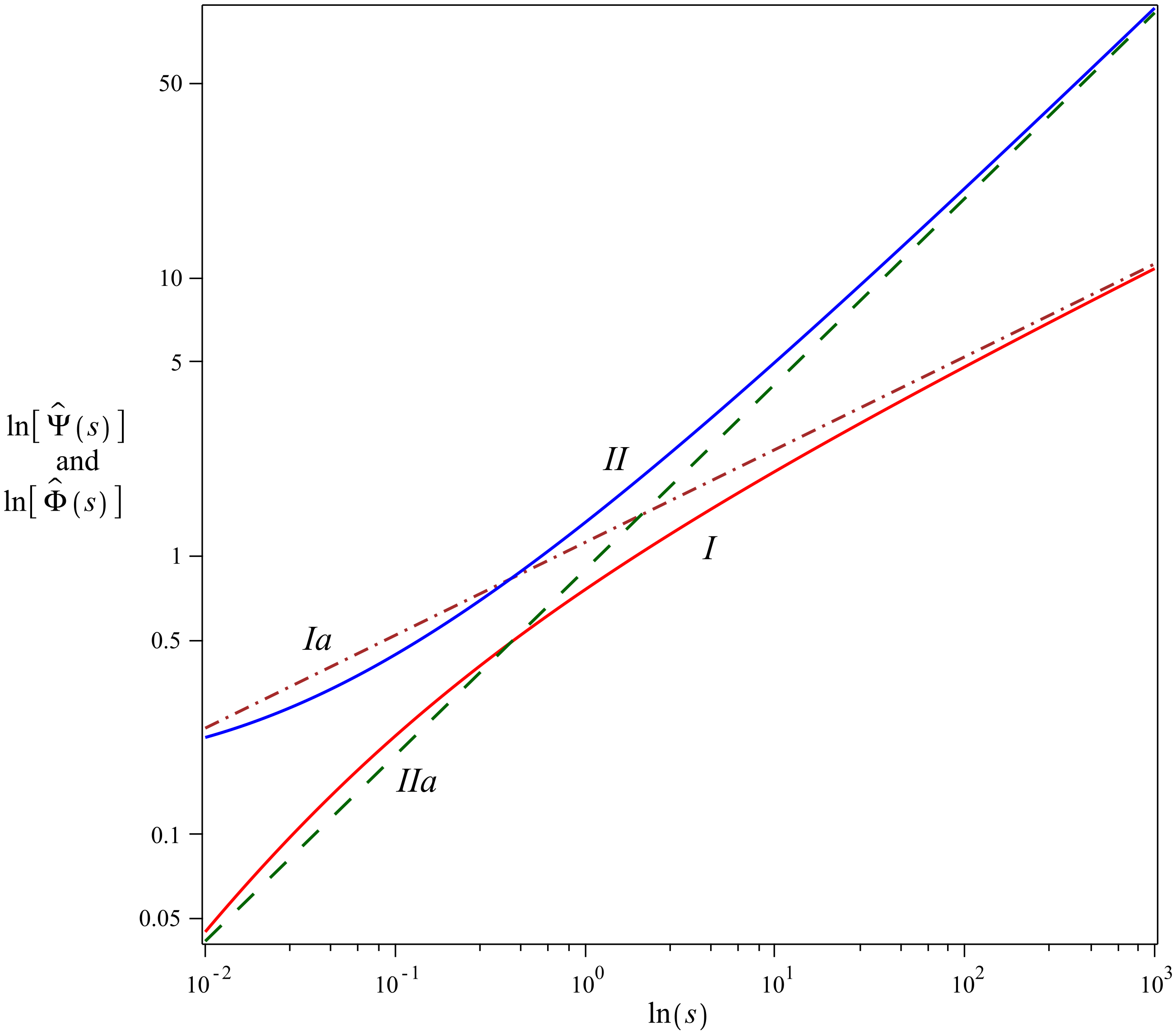
The characteristic exponents for CC relaxation model are given by the power-law functions

$${\widehat{\mathsf{\Psi }}}_{CC}\left(s\right)={\left(s\tau \right)}^{\alpha }\mathrm{and}{\widehat{\mathsf{\Phi }}}_{CC}\left(s\right)={\left(s\tau \right)}^{1-\alpha }$$

(14)

which differ from the asymptotic behavior of ${\widehat{\mathsf{\Psi }}}_{KWW}\left(s\right)$ and ${\widehat{\mathsf{\Phi }}}_{KWW}\left(s\right)$

$${\widehat{\mathsf{\Psi }}}_{A;KWW}\left(s\right)\sim {\left(s\tau \right)}^{\alpha }/\Gamma (1+\alpha )\mathrm{and}{\widehat{\mathsf{\Phi }}}_{A;KWW}\left(s\right)\sim \Gamma (1+\alpha ){\left(s\tau \right)}^{1-\alpha },s\tau \gg 1$$

(15)

only by the factor ${[\Gamma (1+\alpha )]}^{-1}$. Thus, by rescaling Equation (14) we expect the asymptotic agreement with the characteristic functions of the KWW model calculated using Equation (8) or (9). The comparison of ${\widehat{\mathsf{\Psi }}}_{KWW}\left(s\right)$ with ${\widehat{\mathsf{\Psi }}}_{CC}\left(s\right)$, as well as ${\widehat{\mathsf{\Phi }}}_{KWW}\left(s\right)$ with ${\widehat{\mathsf{\Phi }}}_{CC}\left(s\right)$ are presented in Figure 1 where plots are made for $\alpha =1/3$. It is seen that the characteristic exponents ${\widehat{\mathsf{\Psi }}}_{CC}\left(s\right)$ and ${\widehat{\mathsf{\Phi }}}_{CC}\left(s\right)$ match ${\widehat{\mathsf{\Psi }}}_{KWW}\left(s\right)$ and ${\widehat{\mathsf{\Phi }}}_{KWW}\left(s\right)$ for large s. In the opposite case, i.e., for small s, ${\widehat{\mathsf{\Psi }}}_{CC}\left(s\right)$ agrees with ${\widehat{\mathsf{\Phi }}}_{KWW}\left(s\right)$ much better than ${\widehat{\mathsf{\Psi }}}_{KWW}\left(s\right)$. Analogical observation can be made for ${\widehat{\mathsf{\Phi }}}_{CC}\left(s\right)$ which reconstructs ${\widehat{\mathsf{\Psi }}}_{KWW}\left(s\right)$ better than ${\widehat{\mathsf{\Phi }}}_{KWW}\left(s\right)$.

Figure 1. Plot presents the comparison between characteristic functions ${\widehat{\mathsf{\Psi }}}_{KWW}\left(s\right)$ (red solid curve no. I) and ${\widehat{\mathsf{\Psi }}}_{CC}\left(s\right)$ (brown dot-dashed curve no. Ia), as well as between partner functions ${\widehat{\mathsf{\Phi }}}_{KWW}\left(s\right)$ (blue solid curve no. II) and ${\widehat{\mathsf{\Phi }}}_{CC}\left(s\right)$ (green dashed curve no. IIa) for $\alpha =1/3$ and $\tau =1$. The characteristic exponents ${\widehat{\mathsf{\Psi }}}_{KWW}\left(s\right)$ and ${\widehat{\mathsf{\Phi }}}_{KWW}\left(s\right)$ have been calculated using Equation (8) whereas ${\widehat{\mathsf{\Psi }}}_{CC}\left(s\right)$ and ${\widehat{\mathsf{\Phi }}}_{CC}\left(s\right)$ are given by Equation (14). The latter ones are, respectively, multiplied and divided by ${[\Gamma (4/3)]}^{-1}$.

We should also observe that ${\widehat{\mathsf{\Psi }}}_{CC}\left(s\right)$ and ${\widehat{\mathsf{\Phi }}}_{CC}\left(s\right)$, as well as ${\widehat{\mathsf{\Psi }}}_{KWW}\left(s\right)$ and ${\widehat{\mathsf{\Phi }}}_{KWW}\left(s\right)$ are CBFs and by construction satisfy the Sonine condition.

(b)

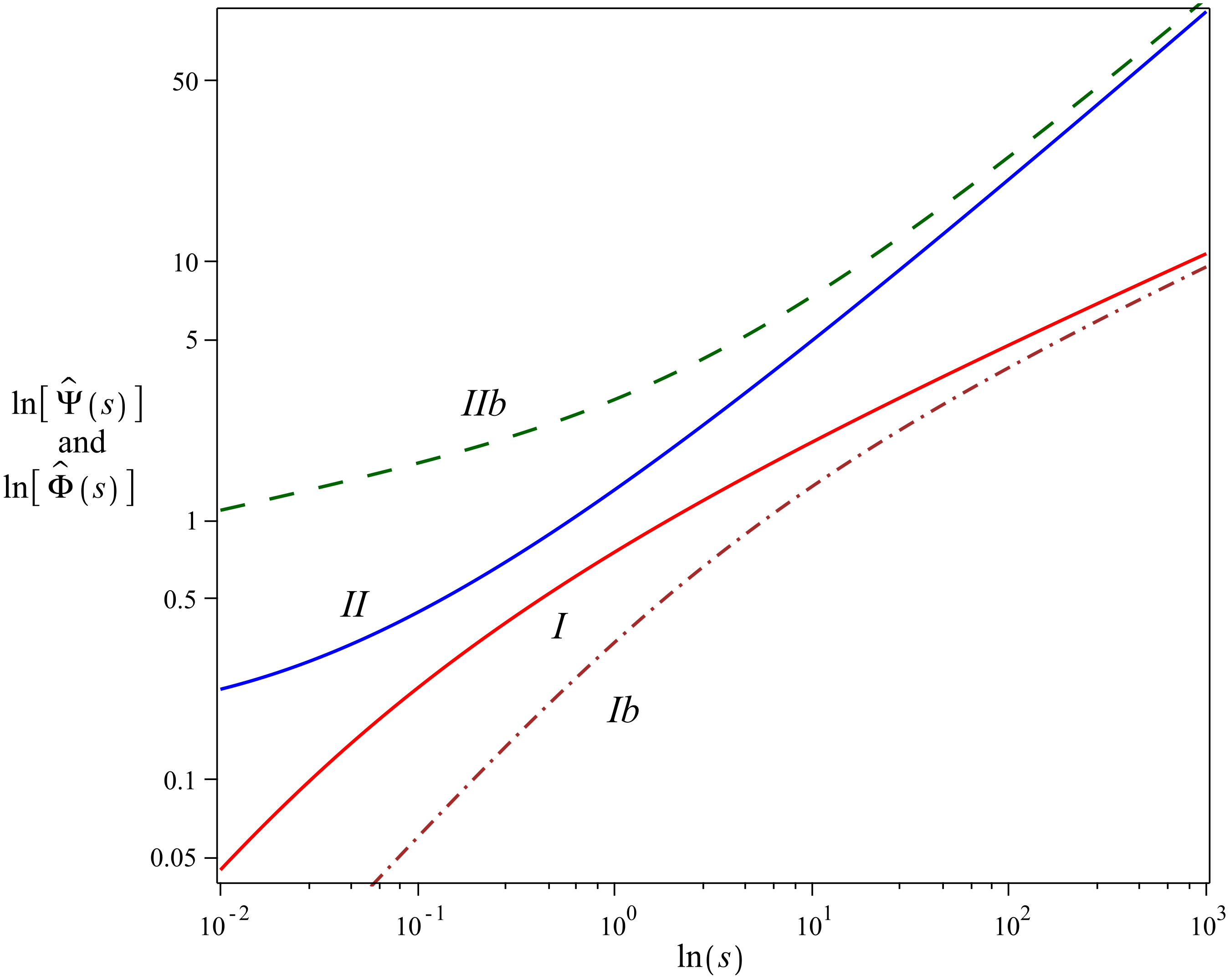
In case of the HN relaxation we have

$${\widehat{\mathsf{\Psi }}}_{HN}\left(s\right)=\{{[1+{\left(s\tau \right)}^{\alpha }]}^{\beta }-1\}\mathrm{and}{\widehat{\mathsf{\Phi }}}_{HN}\left(s\right)=s{\{{[1+{\left(s\tau \right)}^{\alpha }]}^{\beta }-1\}}^{-1}.$$

(16)

For large s the leading asymptotic term of ${\widehat{\mathsf{\Psi }}}_{HN}\left(s\right)$ is ${\left(s\tau \right)}^{\alpha \beta }$. For small s the relevant asymptotics is got if we rewrite ${\widehat{\mathsf{\Psi }}}_{HN}\left(s\right)$ as the series ${\sum }_{r\ge 0}\Gamma (1+\beta ){\left(s\tau \right)}^{\alpha r}/[r!\Gamma (1+\beta -r)]-1$ whose first two terms (i.e., the terms with $r=0$ and $r=1$) give the asymptotics of ${\widehat{\mathsf{\Psi }}}_{HN}\left(s\right)$ proportional to $\beta {\left(s\tau \right)}^{\alpha }$. Gathered together the asymptotic behavior of ${\widehat{\mathsf{\Psi }}}_{HN}\left(s\right)$ reads

$${\widehat{\mathsf{\Psi }}}_{A;HN}\left(s\right)\sim {\left(s\tau \right)}^{\alpha \beta },s\tau \gg 1,\mathrm{and}{\widehat{\mathsf{\Psi }}}_{A;HN}\left(s\right)\sim \beta {\left(s\tau \right)}^{\alpha },s\tau \ll 1$$

(17)

which determine the asymptotics of ${\widehat{\mathsf{\Phi }}}_{HN}\left(s\right)$

$${\widehat{\mathsf{\Phi }}}_{A;HN}\left(s\right)\sim {\left(s\tau \right)}^{1-\alpha }/\beta ,s\tau \gg 1,\mathrm{and}{\widehat{\mathsf{\Phi }}}_{A;HN}\left(s\right)\sim {\left(s\tau \right)}^{1-\alpha \beta },s\tau \ll 1.$$

(18)

As in the previous example also here ${\widehat{\mathsf{\Psi }}}_{A;HN}\left(s\right)$ and ${\widehat{\mathsf{\Phi }}}_{A;HN}\left(s\right)$ are CBFs for $\alpha ,\beta \in (0,1]$. The power-law asymptotics given by Equation (17) for $s\tau \gg 1$ shows that in order to match ${\widehat{\mathsf{\Psi }}}_{KWW}\left(s\right)$ the relations of exponentials ${\alpha }_{HN}{\beta }_{HN}={\alpha }_{KWW}$ has to be satisfied. It means that ${\alpha }_{HN}$ may be chosen arbitrarily if simultaneously ${\beta }_{HN}={\alpha }_{KWW}/{\alpha }_{HN}$. Thus, the small s asymptotics of ${\widehat{\mathsf{\Psi }}}_{A;HN}\left(s\right)$ becomes incompatible with the asymptotics of ${\widehat{\mathsf{\Psi }}}_{A;KWW}\left(s\right)$ and matches it only for $\beta =1$ which is the condition reducing the HN pattern to the CC one. Figure 2, with ${\alpha }_{KWW}=1/3$, ${\alpha }_{HN}=5/6$, and ${\beta }_{HN}=2/5$, shows that for large $\tau s$${\widehat{\mathsf{\Psi }}}_{HN}\left(s\right)$ and ${\widehat{\mathsf{\Phi }}}_{HN}\left(s\right)$ fit well ${\widehat{\mathsf{\Psi }}}_{KWW}\left(s\right)$ and ${\widehat{\mathsf{\Phi }}}_{KWW}\left(s\right)$, respectively, but the matching breaks down for small $s\tau$.

Figure 2. Plot presents the comparison between characteristic exponents ${\widehat{\mathsf{\Psi }}}_{KWW}\left(s\right)$ (red solid curve no. I) and ${\widehat{\mathsf{\Psi }}}_{HN}\left(s\right)$ (brown dot-dashed curve no. Ib), as well as between partner functions ${\widehat{\mathsf{\Phi }}}_{KWW}\left(s\right)$ (blue solid curve no. II) and ${\widehat{\mathsf{\Phi }}}_{HN}\left(s\right)$ (green dashed curve no. IIb). ${\widehat{\mathsf{\Psi }}}_{KWW}\left(s\right)$ and ${\widehat{\mathsf{\Phi }}}_{KWW}\left(s\right)$ are calculated with the help of Equation (8) where we use ${\alpha }_{KWW}=1/3$, $\tau =1$. The characteristic exponents ${\widehat{\mathsf{\Psi }}}_{HN}\left(s\right)$ and ${\widehat{\mathsf{\Phi }}}_{HN}\left(s\right)$ are given by Equation (16) where ${\alpha }_{HN}=5/6$ and ${\beta }_{HN}=2/5$. The comparison between the characteristic functions is made with the factor ${[\Gamma (1+5/6)]}^{-1}$ which is multiplied by ${\widehat{\mathsf{\Psi }}}_{HN}\left(s\right)$ and divided by ${\widehat{\mathsf{\Phi }}}_{HN}\left(s\right)$.

(c)

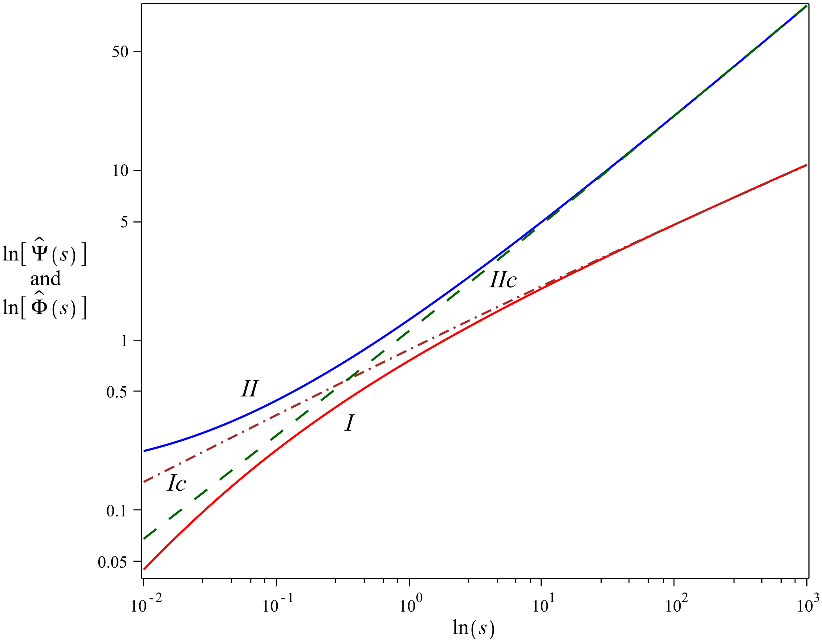
The characteristic exponents of the JWS model are equal to

$${\widehat{\mathsf{\Psi }}}_{JWS}\left(s\right)={\{{[1+{\left(s\tau \right)}^{-\alpha }]}^{\beta }-1\}}^{-1}\mathrm{and}{\widehat{\mathsf{\Phi }}}_{JWS}\left(s\right)=s\{{[1+{\left(s\tau \right)}^{-\alpha }]}^{\beta }-1\}$$

(19)

Their asymptotics read

$$\begin{array}{cc}\hfill {\widehat{\mathsf{\Psi }}}_{A;JWS}\left(s\right)\sim s^{\alpha }/\beta ,s\tau \gg 1,& \mathrm{and}{\widehat{\mathsf{\Psi }}}_{A;JWS}\left(s\right)\sim {\left(s\tau \right)}^{\alpha \beta },s\tau \ll 1,\hfill \end{array}$$

(20)

$$\begin{array}{cc}\hfill {\widehat{\mathsf{\Phi }}}_{A;JWS}\left(s\right)\sim s^{1-\alpha \beta },s\tau \gg 1,& \mathrm{and}{\widehat{\mathsf{\Phi }}}_{A;JWS}\left(s\right)\sim \beta {\left(s\tau \right)}^{1-\alpha },s\tau \ll 1.\hfill \end{array}$$

(21)

As in the previous case also here the asymptotics’ presented by Equation (20) are given by CBFs for $\alpha ,\beta \in (0,1]$. The comparison between ${\widehat{\mathsf{\Psi }}}_{KWW}\left(s\right)$ and ${\widehat{\mathsf{\Psi }}}_{JWS}\left(s\right)$, as well as between ${\widehat{\mathsf{\Phi }}}_{KWW}\left(s\right)$ and ${\widehat{\mathsf{\Phi }}}_{JWS}\left(s\right)$ is shown in Figure 3. It is seen that for large s ${\widehat{\mathsf{\Psi }}}_{JWS}\left(s\right)$ and ${\widehat{\mathsf{\Phi }}}_{JWS}\left(s\right)$ match ${\widehat{\mathsf{\Psi }}}_{KWW}\left(s\right)$ and ${\widehat{\mathsf{\Phi }}}_{KWW}\left(s\right)$ faster than for the CC and HN models. Nevertheless the matchings for small s remain disappointing although at the first glance they seem to be more acceptable than those resulting from the CC and HN models. This, however, may be treated as an artifact coming from the choice of parameters.

Figure 3. Plot presents the comparison between ${\widehat{\mathsf{\Psi }}}_{KWW}\left(s\right)$ (red solid curve no. I) and ${\widehat{\mathsf{\Psi }}}_{JWS}\left(s\right)$ (brown dot-dashed curve no. Ic), as well as between ${\widehat{\mathsf{\Phi }}}_{KWW}\left(s\right)$ (blue solid curve no. II) and ${\widehat{\mathsf{\Phi }}}_{JWS}\left(s\right)$ (green dashed curve no. IIc). ${\widehat{\mathsf{\Psi }}}_{KWW}\left(s\right)$ and ${\widehat{\mathsf{\Phi }}}_{KWW}\left(s\right)$ are calculated with the help of Equation (8) where we use ${\alpha }_{KWW}=1/3$, $\tau =1$. The characteristic exponents ${\widehat{\mathsf{\Psi }}}_{JWS}\left(s\right)$ and ${\widehat{\mathsf{\Phi }}}_{JWS}\left(s\right)$ are given by Equations (16) where ${\alpha }_{JWS}=2/5$, ${\beta }_{JWS}=5/6$, and are, respectively, multiplied and divided by ${[\Gamma (1+2/5)]}^{-1}$.

We complete this section with two remarks:

• The leading order of large s, i.e., short t, asymptotics of all relaxation patterns being considered matches the KWW function.
• In Figure 1, Figure 2 and Figure 3 the curves labelled by I and II show the behavior of various $\widehat{\mathsf{\Psi }}\left(s\right)$ and $\widehat{\mathsf{\Phi }}\left(s\right)$. Unidexed labels I and II characterize plots obtained for the KWW model if $\alpha =1/3$. The labels I and II indexed with subscripts a, b, and c distinguish non-Debye models: a is for the CC, b is for the HN, and c is for the JWS.

5. The Mittag–Leffler Family: Comparison of Useful Properties

5.1. An Interlude: A Few Mathematical Tools

5.1.1. The Efross Theorem as an Integral Decomposition

The Efross theorem [37,38,39,40,41,42] generalizes the Borel convolution theorem for the Laplace transform. According to it, for $\widehat{G}\left(s\right)$ and $\widehat{q}\left(s\right)$ being analytic functions, we have

$$\begin{array}{c}\hfill \begin{array}{cc}\hfill {\mathcal{L}}^{-1}\left[\widehat{G}\left(s\right){\widehat{h}}_1(x,\widehat{q}\left(s\right));t\right]& ={\int }_0^{\infty }{\mathcal{L}}^{-1}[{\widehat{h}}_1(x,s);\xi ]{\mathcal{L}}^{-1}[\widehat{G}\left(s\right){\mathrm{e}}^{-\xi \widehat{q}\left(s\right)};t]\mathrm{d}\xi \hfill \\ \hfill & ={\int }_0^{\infty }{h}_1(x,\xi )h_2(\xi ,t)\mathrm{d}\xi .\hfill \end{array}\end{array}$$

(22)

in which one immediately recognizes the structure of integral decomposition. In the probabilistic language, if $h_1(x,\xi )$ and $h_2(\xi ,t)$ are independent probability distributions, Equation (22) expresses the Bayes theorem and thus may be treated as a joint probability distributions. Namely this identification is made when stochastic methods are applied to the relaxation theory [24]. Within this approach the non-negative random variable $\xi$ is interpreted as an “internal” or operational time which governs the evolution of the function $h_1(x,\xi )={\mathcal{L}}^{-1}[{\widehat{h}}_1(x,s);\xi ]$ bearing the name of the parent process. The second component of the integral decomposition Equation (22) $h_2(\xi ,t)={\mathcal{L}}^{-1}[\widehat{G}\left(s\right){\mathrm{e}}^{-\xi \widehat{q}\left(s\right)};t]$ describes the mutual dependence of operational $\xi$ and physical t times. Unlike regularly clocked physical time t the internal time $\xi$ has the nature of a càdlàg (left continuous right limited) non-negative and non-decreasing stochastic process. According to classification proposed in Ref. [43] and recently reconsidered in Refs. [40,44] both functions $h_i$’s, $i=1,2$, can be either the “safe” or “dangerous” probability densities (PDFs). Sufficient condition to be the “safe” PDF is infinite divisibility, and if it is not the case we may deal with an example of “dangerous” PDF. The working criterion to distinguish the “safe” and “dangerous” cases is their adherence to the class of Bernstein functions. This guarantees that the features characterizing the “safe” PDFs, i.e., non-negativity and infinite divisibility, are satisfied (Appendix D). Remember also that $h_2(\xi ,t)$ should be normalized. For $h_2(\xi ,t)$ being the “safe” PDF we can say that it subordinates $h_1(x,\xi )$. In the opposite case, i.e., for $h_2(\xi ,t)$ being the “dangerous” PDF, we name $h_2(\xi ,t)$ and $h_1(x,\xi )$ the constituents of integral decomposition only.

5.1.2. Integral Decompositions as Subordinations

In the case of relaxation theory we know from Equation (5) that $h_1(x,\xi )$ is independent on x. It is equal to the Debye relaxation function, i.e., $h_1\left(\xi \right)\equiv n_D\left(\xi \right)=exp(-B\xi )$. The latter is CBF as it is the non-negative, normalized, and infinitely divisible with respect to $\xi$. Thus, $n_D\left(\xi \right)$ is the PDF of parent process. The function $h_2(\xi ,t)\equiv h_{2,\mathsf{\Psi }}(\xi ,t)$ involves $\widehat{G}\left(s\right)=\widehat{\mathsf{\Psi }}\left(s\right)/s$, as well as $\widehat{q}\left(s\right)=\widehat{\mathsf{\Psi }}\left(s\right)$ and it is equal to ${\mathcal{L}}^{-1}\{[\widehat{\mathsf{\Psi }}\left(s\right)/s]exp[-\xi \widehat{\mathsf{\Psi }}\left(s\right)];t\}$. Normalization of $h_{2,\mathsf{\Psi }}(\xi ,t)$ in $\xi$ is fulfilled automatically. Because $\widehat{\mathsf{\Psi }}\left(s\right)$ is the characteristic exponent, i.e., it belongs to the class of Bernstein functions, then using Appendix D we can show that $h_{2,\mathsf{\Psi }}(\xi ,t)$ is “safe” PDF and it subordinates the Debye relaxation process $h_1\left(\xi \right)$. With the help of Efross theorem Equation (22) $n\left(t\right)$ can be written as

$$\begin{array}{c}\hfill \begin{array}{cc}\hfill n\left(t\right)& ={\int }_0^{\infty }{\mathcal{L}}^{-1}[{\widehat{n}}_D\left(s\right);\xi ]{\mathcal{L}}^{-1}\left[\frac{\widehat{\mathsf{\Psi }}\left(s\right)}{s}{\mathrm{e}}^{-\xi \widehat{\mathsf{\Psi }}\left(s\right)};t\right]\mathrm{d}\xi \hfill \\ \hfill & ={\mathcal{L}}^{-1}\left[\frac{\widehat{\mathsf{\Psi }}\left(s\right)}{s}{\widehat{n}}_D\left(\widehat{\mathsf{\Psi }}\left(s\right)\right);t\right],\hfill \end{array}\end{array}$$

(23)

where ${\widehat{n}}_D\left(s\right)=\mathcal{L}[n_D\left(t\right);s]={(B+s)}^{-1}$. For $\widehat{\mathsf{\Psi }}\left(s\right)$ being CBF there exists associated CBF $\widehat{\mathsf{\Phi }}\left(s\right)$, such that $\widehat{\mathsf{\Psi }}\left(s\right)\widehat{\mathsf{\Phi }}\left(s\right)=s$. Thus, Equation (23) can be written down in its alternative form

$$\begin{array}{c}\hfill \begin{array}{cc}\hfill n\left(t\right)& ={\mathcal{L}}^{-1}\left\{{\left[\widehat{\mathsf{\Phi }}\left(s\right)\right]}^{-1}{\widehat{n}}_D\left(s/\widehat{\mathsf{\Phi }}\left(s\right)\right);t\right]\hfill \\ \hfill & ={\int }_0^{\infty }{\mathcal{L}}^{-1}[{\widehat{n}}_D\left(s\right);\xi ]{\mathcal{L}}^{-1}\left\{{\left[\widehat{\mathsf{\Phi }}\left(s\right)\right]}^{-1}{\mathrm{e}}^{-\xi s/\widehat{\mathsf{\Phi }}\left(s\right)};t\right\}\mathrm{d}\xi ,\hfill \end{array}\end{array}$$

(24)

where $h_2(\xi ,t)\equiv h_{2,\mathsf{\Phi }}(\xi ,t)={\mathcal{L}}^{-1}\{exp[-\xi s/\widehat{\mathsf{\Phi }}\left(s\right)]/\widehat{\mathsf{\Phi }}\left(s\right);t\}$ subordinates the Debye relaxation process as well. This duality is not problematic-both characteristic functions $\mathsf{\Psi }\left(s\right)$ and $\mathsf{\Phi }\left(s\right)$ lead to the same $n\left(t\right)$ if $\widehat{\mathsf{\Psi }}\left(s\right)\widehat{\mathsf{\Phi }}\left(s\right)=s$ which once more emphasizes the importance of the Sonine condition. Additionally, by virtue of considerations presented in Section 2 (cf. Equation (5)), we know that $h_{2,\mathsf{\Psi }}(\xi ,t)$ and $h_{2,\mathsf{\Phi }}(\xi ,t)$ are always the “safe” PDFs. Thus they may be used to subordinate the Debye relaxation, as well as other “safe” distributions, e.g., the normal distribution, cf. Ref. [28]. We can also use another subordinators, e.g., ${\mathcal{L}}^{-1}\{s^{\alpha \gamma -\beta }exp[-u{s}^{\alpha }];t\}$, which subordinates the CD relaxation model. The example of using two kinds of subordinators is presented in Ref. [40].

5.1.3. Subordinations as Signposts Leading to Evolution Equations

The subordination approach allows one to find the evolution equations which govern the behavior of subordinated parent process [43]; this we have named the relaxation function $n\left(t\right)$. To obtain suitable equations we need two building blocks. The first of them is the standard evolution equation for $n_D\left(t\right)$, but considered in the Laplace space and with s replaced by $\widehat{\mathsf{\Psi }}\left(s\right)$. The second one is the relation ${\widehat{n}}_D\left(\widehat{\mathsf{\Psi }}\left(s\right)\right)=s\widehat{n}\left(s\right)/\widehat{\mathsf{\Psi }}\left(s\right)$ derived from Equation (23).

The evolution equation (with respect to time t) of $n_D\left(t\right)$ is well-known. It reads ${\dot{n}}_D\left(t\right)=-B{n}_D\left(t\right)$ and in the Laplace space equals to

$$s{\widehat{n}}_D\left(s\right)-n_D\left(0\right)=-B{\widehat{n}}_D\left(s\right)$$

(25)

with the initial condition $n_D\left(0\right)=1$. After replacing s by $\widehat{\mathsf{\Psi }}\left(s\right)$ we have

$$\widehat{\mathsf{\Psi }}\left(s\right){\widehat{n}}_D\left(\widehat{\mathsf{\Psi }}\left(s\right)\right)-1=-B{\widehat{n}}_D\left(\widehat{\mathsf{\Psi }}\left(s\right)\right).$$

(26)

Setting ${\widehat{n}}_D\left(\widehat{\mathsf{\Psi }}\left(s\right)\right)=s\widehat{n}\left(s\right)/\widehat{\mathsf{\Psi }}\left(s\right)$ and substituting it into Equation (26) we get

$$\widehat{n}\left(s\right)=s^{-1}-B{\left[\widehat{\mathsf{\Psi }}\left(s\right)\right]}^{-1}\widehat{n}\left(s\right),$$

(27)

which can be rewritten as

$$\frac{\widehat{\mathsf{\Psi }}\left(s\right)}{s}[s\widehat{n}\left(s\right)-1]=-B\widehat{n}\left(s\right).$$

(28)

Taking the inverse Laplace transform of Equations (27) and (28) in which we use the Laplace convolution we get, respectively,

$$n\left(t\right)=1-B{\int }_0^{t}M(t-u)n\left(u\right)\mathrm{d}u\mathrm{and}{\int }_0^{t}k(t-u)\dot{n}\left(u\right)\mathrm{d}u=-Bn\left(t\right),$$

(29)

where

$$M\left(t\right)={\mathcal{L}}^{-1}[\widehat{M}\left(s\right);t]\mathrm{with}\widehat{M}\left(s\right)={\left[\widehat{\mathsf{\Psi }}\left(s\right)\right]}^{-1},$$

(30)

and

$$k\left(t\right)={\mathcal{L}}^{-1}[\widehat{k}\left(s\right);t]\mathrm{with}\widehat{k}\left(s\right)={[\widehat{\mathsf{\Psi }}\left(s\right)/s]}^{-1}={\left[\widehat{\mathsf{\Phi }}\left(s\right)\right]}^{-1}.$$

(31)

The functions $M\left(t\right)$ and $k\left(t\right)$ are non-negative and can be interpreted as memory functions or kernels. Because $\widehat{\mathsf{\Psi }}\left(s\right)$ is CBF then $\widehat{M}\left(s\right)$ is the Stieltjes function (SF) and $s/\widehat{\mathsf{\Psi }}\left(s\right)$ is also CBF, see Appendix B. Denoting the latter as $\widehat{\mathsf{\Phi }}\left(s\right)$ we learn that $\widehat{k}\left(s\right)$ is also SF [27,45,46]. The relation $\widehat{\mathsf{\Psi }}\left(s\right)\widehat{\mathsf{\Phi }}\left(s\right)=s$ indicates that $\widehat{M}\left(s\right)\widehat{k}\left(s\right)=s^{-1}$ which means that the memory functions $M\left(t\right)$ and $k\left(t\right)$ fulfill the Sonine equation

$${\int }_0^{t}M(t-u)k\left(u\right)\mathrm{d}u={\int }_0^{t}M\left(u\right)k(t-u)\mathrm{d}u=1.$$

(32)

Equation (29) express the time-smeared evolution, either of the relaxation function or its derivative. Detailed discussion of mutual relation between these equations has been presented in [27,46]. From the physical point of view the first equation present in the pair (29) is known as the master equation and may be considered as general modeling of the memory dependent linear evolution scheme. Equation (29) are both the Volterra type integral equations [4]. For some special choices of the kernel $k\left(t\right)$ the second of them specializes to the fractional differential equations. However, ulility of Equation (29) goes far beyond the well-established fractional analysis approach to the relaxation phenomena [18,45].

5.2. Examples

As noticed, Equations (23) and (24) yield the same results as governed by equivalent Equation (29). Thus, the relaxation function $n\left(t\right)$ can be derived with the help either of Equations (23) or (24). Without loss of generality we take Equation (23) with the characteristic function $\widehat{\mathsf{\Psi }}\left(s\right)$ presented in Section 3 to describe the evolution of $n\left(t\right)$.

To derive $n\left(t\right)$ for any among the non-Debye relaxation models listed in Section 3 we will use the formula

$${\mathcal{L}}^{-1}[s^{\alpha \gamma -\beta }{\mathrm{e}}^{-u{s}^{\alpha }};t]=\frac{\Gamma \left(\gamma \right)t^{\beta }}{\alpha u^{\gamma }}{g}_{\alpha ,\beta }^{\gamma }(u,t)$$

(33)

obtained from [47] (Equations (5) and (6)) with the help of the second formula in Equation (A4). The function $g_{\alpha ,\beta }^{\gamma }(u,t)$ is connected to its one variable version $g_{\alpha ,\beta }^{\gamma }\left(x\right)$ through Equation (A5). Equation (33) generalizes the known formula ${\mathcal{L}}^{-1}[s^{\alpha -1}{\mathrm{e}}^{-u{s}^{\alpha }};t]=t{g}_{\alpha }(u,t)/\left(\alpha u\right)$ appearing for the one-parameter Mittag-Leffer function [39,40,48]. Indeed, Equation (33) reduces to it for $\gamma =\beta =1$. Having all this at hands we are ready to find relaxation functions looked for.

(i)

For the CC model, for which ${\widehat{\mathsf{\Psi }}}_{CC}\left(s\right)$ is given by Equation (14) multiplied by B, we have

$$\begin{array}{c}\hfill \begin{array}{cc}\hfill n_{CC}\left(t\right)& ={\int }_0^{\infty }{\mathrm{e}}^{-Bu}{\mathcal{L}}^{-1}[B{\tau }^{\alpha }{s}^{\alpha -1}{\mathrm{e}}^{-uB{\tau }^{\alpha }{s}^{\alpha }};t]\mathrm{d}u\hfill \\ \hfill & ={\int }_0^{\infty }{\mathrm{e}}^{-{\tau }^{-\alpha }\xi }{\mathcal{L}}^{-1}[s^{\alpha -1}{\mathrm{e}}^{-\xi s^{\alpha }};t]\mathrm{d}\xi ,\hfill \end{array}\end{array}$$

(34)

where we set $uB{\tau }^{\alpha }=\xi$. We say that ${\mathcal{L}}^{-1}[s^{\alpha -1}{\mathrm{e}}^{-\xi s^{\alpha }};t]$ subordinates the Debye case. Using Equation (33) for $\gamma =\beta =1$ we get Equation (A1) with $a={\tau }^{-\alpha }$ and $p=t$ and

$$n_{CC}\left(t\right)=E_{\alpha }[-{(t/\tau )}^{\alpha }],$$

(35)

which is well-known relaxation function of the CC model [18,21,29,30]. Asymptotics of $n_{CC}\left(t\right)$ for t being smaller or larger than $\tau$ can be obtained from the first terms of the series representations given in Refs. [18,29,30]. The results read

$$n_{A;CC}\left(t\right)\sim 1-\frac{{(t/\tau )}^{\alpha }}{\Gamma (1+\alpha )},t\ll \tau ,\mathrm{and}{n}_{A;CC}\left(t\right)\sim \frac{{(t/\tau )}^{-\alpha }}{\Gamma (1-\alpha )},t\gg \tau .$$

(36)

The short time asymptotics given by the first equation in Equation (36) constitutes also the first two terms of the stretched exponential $exp[-t^{\alpha }/\Gamma (1+\alpha )]$. Such approximation was proposed in Ref. [49] and it offers good results for low values of $\alpha$ at sufficiently short times.

The evolution equations derived from Equation (29) read

$$n_{CC}\left(t\right)=1-{\tau }^{-1}\left(I^{\alpha }{n}_{CC}\right)\left(t\right)\mathrm{and}\left({}^c{D}^{\alpha }{n}_{CC}\right)\left(t\right)=-{\tau }^{\alpha }{n}_{CC}\left(t\right),$$

(37)

where the symbol $\left(I^{1-\alpha }\frac{\mathrm{d}}{\mathrm{d}x}f\right)\left(x\right)$ denotes the fractional integral defined in Appendix E for $\alpha \in (0,1)$ while ${}^c{D}^{\alpha }$ is the fractional (Caputo) derivative operator. Equations (37) are equivalent to [50] (Equation (3.7.43)) and [18] (Equation (3.10)), respectively.

(ii)

Our next example is the HN relaxation function. We begin with the subordination approach which involves the Debye relaxation and ${\mathcal{L}}^{-1}\{\widehat{\mathsf{\Psi }}\left(s\right)exp[-\xi \widehat{\mathsf{\Psi }}\left(s\right)]/s;t\}$. Substituting Equation (16) multiplied by B into Equation (23) we get

$$n_{HN}\left(t\right)=B{\int }_0^{\infty }{\mathcal{L}}^{-1}\{B{s}^{-1}[{\tau }^{\alpha \beta }{({\tau }^{-\alpha }+s^{\alpha })}^{\beta }-1]{\mathrm{e}}^{-\xi B{\tau }^{\alpha \beta }{({\tau }^{-\alpha }+s^{\alpha })}^{\beta }};t\}\mathrm{d}\xi ,$$

(38)

where $n_D\left(\xi \right)$ is cancelled by $exp(-B\xi )$ coming from ${\widehat{\mathsf{\Psi }}}_{HN}\left(s\right)$. Next, we apply once more the Efross theorem to the inverse Laplace transform in Equation (38), this time with $\widehat{G}\left(s\right)=s^{-1}$ and $\widehat{q}\left(s\right)={\tau }^{-\alpha }+s^{\alpha }$ put in. Thus, we can express Equation (38) as

$$\begin{array}{c}\hfill \begin{array}{cc}\hfill n_{HN}\left(t\right)& =B{\int }_0^{\infty }\left\{{\int }_0^{\infty }{\mathcal{L}}^{-1}[({\tau }^{\alpha \beta }{s}^{\beta }-1){\mathrm{e}}^{-\xi B{\tau }^{\alpha \beta }{s}^{\beta }};u]{\mathrm{e}}^{-u{\tau }^{-\alpha }}{\mathcal{L}}^{-1}[s^{-1}{\mathrm{e}}^{-u{s}^{\alpha }};t]\mathrm{d}u\right\}\mathrm{d}\xi \hfill \\ \hfill & =B{\int }_0^{\infty }{\mathcal{L}}^{-1}\left[({\tau }^{\alpha \beta }{s}^{\beta }-1){\int }_0^{\infty }{\mathrm{e}}^{-\xi B{\tau }^{\alpha \beta }{s}^{\beta }}\mathrm{d}\xi ;u\right]{\mathcal{L}}^{-1}[s^{-1}{\mathrm{e}}^{-u({\tau }^{-\alpha }+s^{\alpha })};t]\mathrm{d}u\hfill \\ \hfill & ={\int }_0^{\infty }{\mathrm{e}}^{-u{\tau }^{-\alpha }}{\mathcal{L}}^{-1}[s^{-\beta }(s^{\beta }-{\tau }^{-\alpha \beta });u]{\mathcal{L}}^{-1}[s^{-1}{\mathrm{e}}^{-u{s}^{\alpha }};t]\mathrm{d}u.\hfill \end{array}\end{array}$$

(39)

Because of ${\mathcal{L}}^{-1}[s^{-\beta }(s^{\beta }-{\tau }^{-\alpha \beta });u]=\delta \left(u\right)-{\tau }^{-\alpha \beta }{u}^{\beta -1}/\Gamma \left(\beta \right)$ we rewrite Equation (39) as

$$\begin{array}{cc}\hfill n_{HN}\left(t\right)& =1-{\tau }^{-\alpha \beta }{\int }_0^{\infty }{\mathrm{e}}^{-{\tau }^{-\alpha }u}\frac{u^{\beta -1}}{\Gamma \left(\beta \right)}{\mathcal{L}}^{-1}[s^{-1}{\mathrm{e}}^{-u{s}^{\alpha }};t]\mathrm{d}u\hfill \end{array}$$

(40)

$$\begin{array}{cc}\hfill & =1-{(t/\tau )}^{\alpha \beta }{\int }_0^{\infty }{\mathrm{e}}^{-{\tau }^{-\alpha }u}\frac{t}{\alpha u}{g}_{\alpha ,1+\alpha \beta }^{\beta }(u,t)\mathrm{d}u.\hfill \end{array}$$

(41)

From Equation (33) it comes out that ${\mathcal{L}}^{-1}[s^{-1}{\mathrm{e}}^{-u{s}^{\alpha }};t]=\Gamma \left(\beta \right)t^{1+\alpha \beta }/\left(\alpha u^{\beta }\right)g_{\alpha ,1+\alpha \beta }^{\beta }(u,t)$. Then, with the help of Equation (A4), we get

$$n_{HN}\left(t\right)=1-{(t/\tau )}^{\alpha \beta }{E}_{\alpha ,1+\alpha \beta }^{\beta }[-{(t/\tau )}^{\alpha }],$$

(42)

which is usually obtained by employing ${\widehat{\varphi }}_{HN}\left(\mathrm{i}\omega \right)$, Equations (A6) and (1) as it is presented in [18,29,30,51]. Notice that, due to ([18] Equation (3.13)) we have

$${\mathrm{e}}^{-{\tau }^{-\alpha }u}\frac{u^{\beta -1}}{\Gamma \left(\beta \right)}={\tau }^{\alpha \beta }{\mathcal{L}}^{-1}[{(1+s{\tau }^{\alpha })}^{-\beta };t],$$

(43)

proportional to the spectral function of CD model which now generates the parent process. Hence, looking on Equations (40) and (43) we can say that the CD relaxation together with ${\mathcal{L}}^{-1}[s^{-1}exp(-u{s}^{\alpha });t]$ are the constituents of the integral decomposition of $1-n_{HN}\left(t\right)$. From [18,29,30] we know that the short and long time power-law asymptotics of $n_{HN}\left(t\right)$ are equal to

$$n_{A;HN}\left(t\right)\sim 1-\frac{{(t/\tau )}^{\alpha \beta }}{\Gamma (1+\alpha \beta )},t\ll \tau ,\mathrm{and}{n}_{A;HN}\left(t\right)\sim \frac{\beta {(t/\tau )}^{-\alpha }}{\Gamma (1-\alpha )},t\gg \tau .$$

(44)

The evolution equation is equal to ([18] Equations (3.40) and (3.50))

$${}^{\mathrm{C}}{(D^{\alpha }+{\tau }^{-\alpha })}^{\beta }{n}_{HN}\left(t\right)=-{\tau }^{\alpha \beta },$$

(45)

where the pseudo-operator ${}^{\mathrm{C}}{(D^{\alpha }+{\tau }^{-\alpha })}^{\beta }$ is defined in Appendix E.

(iii)

Equation (23) for the JWS model gives

$$n_{JWS}\left(t\right)=B{\int }_0^{\infty }{\mathcal{L}}^{-1}\left[\frac{s^{\alpha \beta -1}}{{(s^{\alpha }+{\tau }^{-\alpha })}^{\beta }-s^{\alpha \beta }}{\mathrm{e}}^{-\xi B\frac{{(s^{\alpha }+{\tau }^{-\alpha })}^{\beta }}{{(s^{\alpha }+{\tau }^{-\alpha })}^{\beta }-s^{\alpha \beta }}};t\right]\mathrm{d}\xi ,$$

(46)

which after using once again the Efross theorem where $\widehat{G}\left(s\right)=s^{\alpha \beta -1}$ and $\widehat{q}\left(s\right)=s^{\alpha }+{\tau }^{-\alpha }$ can be represented as

$$\begin{array}{c}\hfill \begin{array}{cc}\hfill n_{JWS}\left(t\right)& =B{\int }_0^{\infty }\left\{{\int }_0^{\infty }{\mathcal{L}}^{-1}\left[\frac{1}{s^{\beta }-{(s-{\tau }^{-\alpha })}^{\beta }}{\mathrm{e}}^{-\xi B\frac{s^{\beta }}{s^{\beta }-{(s-{\tau }^{-\alpha })}^{\beta }}};u\right]\right.\hfill \\ & \left.\times {\mathcal{L}}^{-1}[s^{\alpha \beta -1}{\mathrm{e}}^{-u({\tau }^{-\alpha }+s^{\alpha })};t]\mathrm{d}u\right\}\mathrm{d}\xi .\hfill \end{array}\end{array}$$

(47)

Calculating the integral over $\xi$ (as it was done in the example (ii)) we can simplify the first inverse Laplace transform. It enables us to write down the above equation in the form

$$\begin{array}{c}\hfill \begin{array}{cc}\hfill n_{JWS}\left(t\right)& ={\int }_0^{\infty }{\mathcal{L}}^{-1}[s^{-\beta };u]{\mathrm{e}}^{-u{\tau }^{-\alpha }}{\mathcal{L}}^{-1}[s^{\alpha \beta -1}{\mathrm{e}}^{-u{s}^{\alpha }};t]\mathrm{d}u\hfill \\ \hfill & ={\int }_0^{\infty }{\mathrm{e}}^{-u{\tau }^{-\alpha }}{u}^{\beta -1}/\Gamma \left(\beta \right){\mathcal{L}}^{-1}[s^{\alpha \beta -1}{\mathrm{e}}^{-u{s}^{\alpha }};t]\mathrm{d}u\hfill \\ \hfill & ={\int }_0^{\infty }{\mathrm{e}}^{-{\tau }^{-\alpha }}\frac{t}{\alpha u}{g}_{\alpha ,1}^{\beta }(t,u)=E_{\alpha ,1}^{\beta }[-{(t/\tau )}^{\alpha }].\hfill \end{array}\end{array}$$

(48)

To show that ${\mathcal{L}}^{-1}[s^{\alpha \beta -1}{\mathrm{e}}^{-u{s}^{\alpha }};t]=\Gamma \left(\beta \right)t/\left(\alpha u^{\beta }\right)g_{\alpha ,1}^{\beta }(u,t)$ we employ Equation (33). Next, using Equation (43) we express $n_{JWS}\left(t\right)$ as

$$n_{JWS}\left(t\right)={\int }_0^{\infty }{\mathcal{L}}^{-1}[{({\tau }^{-\alpha }+s^{\alpha })}^{-\beta };u]{\mathcal{L}}^{-1}[s^{\alpha \beta -1}{\mathrm{e}}^{-u{s}^{\alpha }};t]\mathrm{d}u,$$

(49)

which means that to obtain the relaxation function of the JWS model we can use two kinds of subordination approaches. Using the different subordinators we can subordinate the Debye or CD process. Thus, the processes which lead to the JWS relaxation model can be obtained using various approaches. The asymptotic behavior of $n_{JWS}\left(t\right)$ can be given by

$$n_{A;JWS}\left(t\right)\sim 1-\frac{\beta {(t/\tau )}^{\alpha }}{\Gamma (1+\alpha )},t\ll \tau ,\mathrm{and}{n}_{A;JWS}\left(t\right)\sim \frac{\beta {(t/\tau )}^{-\alpha \beta }}{\Gamma (1-\alpha \beta )},t\gg \tau .$$

(50)

Its evolution equation reads

$${(D^{\alpha }+{\tau }^{-\alpha })}^{\beta }{n}_{JWS}\left(t\right)=\frac{t^{\alpha \beta }}{\Gamma (1-\alpha \beta )}.$$

(51)

Appendix E contains the definition of the pseudo-operator ${(D^{\alpha }+{\tau }^{-\alpha })}^{\beta }$. Equation (51) has been discussed in [52] (Equation (4.3)) and justified by the so-called under- and overshooting subordination technique applied for the anomalous diffusion.

Analyzing the above examples we see that the integral decomposition Equation (22) can be interpreted as an alternative form of Equation (1) obtained from Equation (5) by employing Equation (11). It provides us also a missing long-time asymptotics of the KWW relaxation model Equation (2). The relevant asymptotic behavior for short and long times is

$$n_{KWW}\left(t\right)\sim 1-{(t/\tau )}^{\alpha },t\ll \tau ,\mathrm{and}{n}_{KWW}\left(t\right)\sim exp[-{(t/\tau )}^{\alpha }],t\gg \tau ,$$

(52)

obtained in Refs. [29,30].

Looking at the asymptotics of CC and JWS relaxation functions we see that for short times they have similar power-law behavior as $n_{KWW}\left(t\right)$, albeit they differ by a constant. The HN relaxation function differs more significantly, the exponential involves two parameters and to bring the asymptotics to agreement we have to put in restrictive condition ${\alpha }_{HN}{\beta }_{HN}={\alpha }_{KWW}$. An analogous, but reverse situation we met when wanting to create agreement between the asymptotics for large t. This leads to the conclusion that going beyond the short time asymptotics one has to be careful with choosing one of the Mittag–Leffler functions as an object suitable to replace the KWW function. In order to make the proper choice it is necessary to have information concerning the middle and long-time behavior of the relaxation function.

6. Conclusions

It is known that the KWW function does not describe properly many relaxation phenomena. It is much better (and still friendly in practice) is to use the CC model. However, this model also breaks down in many physically interesting cases: this was the reason of introducing the HN and JWS models as phenomenological schemes fit the data in the frequency domain. If transformed to the time domain, both these models lead to the time decay laws given in terms of multiparameter Mittag–Leffler functions, until recently unfamiliar to the physicists’ community. Simultaneously information on the time decay of dielectric polarization is often much more needed for practical applications than data obtained in the spectroscopy experiments. The latter are more precise and cover larger range of the frequency involving 10 or even more orders of magnitude but they are not easy to be translated to the time domain. A fear of using scary looking special functions of the Mittag–Leffler family effectively discourages a vast majority of physicists, firt of all the experimentalists. As the consequences it causes that they consider fitting the data by the stretched exponential function not as a routine coming from the long-time habit but as a method which is the only doable procedure. We consider this situation perplexing and propose to give up this long-time habit. Having in mind that functions describing the relaxation phenomena are rather unknown, we propose to begin with analysis of the characteristic exponents expressed in terms of easily calculable functions. Properties of these functions illustrate the problems we face when comparing various theoretical schemes used in the relaxation theory, in particular the problem of choosing the most suitable relaxation pattern. As a benchmark for comparing different relaxation patterns, we took the stretched exponential and collated it, one by one, with well established models: CC, HN, and JWS. These models are significantly different and overlap only in the asymptotic regime of large s, i.e., at short times. Nevertheless we do not consider this result valueless—it only gives a warning that there is a need for additional information, e.g., the higher order short time asymptotics of relaxation functions or their long-time behavior. Tools to be used in order to push forward as such investigations are collected and listed in the Section 5. Thus our main conclusion is that both theoretical studies, as well as the time domain measurements of polarization decays, should go beyond the stretched exponential fit and should use more extensively the results obtained by spectroscopy methods translated to the time domain. Here, we would like to emphasize that Mittag–Leffler functions are well manageable with standard computer algebra packages, such as Mathematica, Matlab and Maple, and it is not a significant problem to familiarize oneself with them.

References

- Böttcher, C.J.F.; Bordewijk, P. Theory of Electric Polarization; Elsevier: Amsterdam, The Netherlands, 1996; Volume 2. [Google Scholar]
- Johnston, D.C. Stretched exponential relaxation arising from continuous sum of exponential decays. Phys. Rev. B 2006, 74, 184430. [Google Scholar] [CrossRef] [Green Version]
- Pollard, H. The Bernstein-Widder theorem on completely monotonic functions. Duke Math. J. 1944, 11, 427–430. [Google Scholar] [CrossRef]
- Grippenberg, G.; Londen, S.O.; Staffans, O.J. Volterra Integral and Functional Equations; Cambridge University Press: Cambridge, UK, 1990. [Google Scholar]
- Luneburg, R.K. Mathematical Theory of Optics; University of California Press: Berkeley, CA, USA; Los Angeles, CA, USA, 1966; Chapter II. [Google Scholar]
- Maxwell, J.C. The Scientific Papers; Dover: New York, NY, USA, 1952. [Google Scholar]
- Makowski, A.J.; Górska, K. Quantization of the Maxwell fish-eye problem and the quantum-classical correspondence. Phys. Rev. A 2009, 79, 052116. [Google Scholar] [CrossRef]
- Gettens, R.T.T.; Gilbert, J.L. The electrochemical impedance of polarized 316L stainless steel: Structure-property-adsorption correlation. J. Biomed. Mater. Res. A 2008, 90, 121–132. [Google Scholar] [CrossRef] [PubMed]
- Haeri, M.; Goldberg, S.; Gilbert, J.L. The voltage-dependent electrochemical impedance spectroscopy of CoCrMo medical alloy using time-domain techniques: Generalized Cauchy-Lorentz, and KWW-Randles functions describing non-ideal interfacial behaviour. Corros. Sci. 2011, 53, 582–588. [Google Scholar] [CrossRef]
- Hernández-Balaguera, E.; Polo, J.L. A generalized procedure for the coulostatic method using a constant phase element. Electro. Acta 2017, 233, 167–172. [Google Scholar] [CrossRef]
- Hernández-Balaguera, E.; Polo, J.L. On the potential-step hold time when the transient-current response exhibits a Mittag-Leffler decay. J. Electro. Chem. 2020, 856, 113631. [Google Scholar] [CrossRef]
- Hernández-Balaguera, E. Coulostatics in bielectrochemistry; A physical interpretation of the electrode-tissue processes from the theory of fractional calculus. Chaos Solitons Fractals 2021, 145, 110768. [Google Scholar] [CrossRef]
- Hernández-Balaguera, E. Numerical approximations on the transient analysis of bioelectric phenomena at long time scales. Chaos Solitons Fractals 2021, 145, 110787. [Google Scholar] [CrossRef]
- Hernández-Balaguera, E.; Del Pozo, G.; Arredondo, B.; Romero, B.; Pereyra, C.; Xie, H.; Lira-Cantú, M. Unraveling the Key Relationship between Perovskite Capacitive Memory, Long Timescale Cooperative Relaxation Phenomena, and Anomalous J-V Hysteresis. Solar RRL 2021, 5, 2000707. [Google Scholar] [CrossRef]
- Alvarez, F.; Alegría, A.; Colmenero, J. Relationship between the time-domain Kohlrausch-Williams-Watts and frequency-domain Havriliak-Negami relaxation functions. Phys. Rev. B 1991, 44, 7306–7312. [Google Scholar] [CrossRef]
- Alvarez, F.; Alegría, A.; Colmenero, J. Interconnection between frequency-domain Havriliak-Negami and time-domain Kohlrausch-Williams-Watts relaxation functions. Phys. Rev. B 1993, 47, 125–130. [Google Scholar] [CrossRef] [PubMed]
- Havriliak, S., Jr.; Havriliak, S.J. Comparison of the Havriliak-Negami and stretched exponential functions. Polymers 1996, 37, 4107–4110. [Google Scholar] [CrossRef]
- Garrappa, R.; Mainardi, F.; Maione, G. Models of dielectric relaxation based on completely monotone functions. Frac. Calc. Appl. Anal. 2016, 19, 1105–1160. [Google Scholar] [CrossRef] [Green Version]
- Metzler, R.; Klafter, J. From stretched exponential to inverse power-law: Fractional dynamics, Cole-Cole relaxation processes, and beyond. J. Non-Cryst. Solids 2002, 305, 81–87. [Google Scholar] [CrossRef]
- Stanislavsky, A.; Weron, K. Fractional-calculus tools applied to study the nonexponential relaxation in dielectrics. In Handbook of Fractional Calculus with Applications. Volume 5. Applications in Physics, Part B; Tarasov, V.E., Ed.; De Gruyter: Berlin, Germany, 2019. [Google Scholar]
- Weron, K.; Kotulski, M. On the Cole-Cole relaxation function and related Mittag-Leffler distribution. Phys. A 1996, 232, 180–188. [Google Scholar] [CrossRef]
- Schilling, R.L. An introduction to Lévy and Feller processes. In From Lévy–Type Processes to Parabolic SPDEs. Advanced Courses Mathematics Birkhäuser; Springer: Cham, Germany, 2016; pp. 1–126. [Google Scholar]
- Baule, A.; Friedrich, R. Joint probability distribution for a class on non-Markovian processes. Phys. Rev. 2003, 71, 026101. [Google Scholar] [CrossRef] [Green Version]
- Fogedby, H.C. Langevin equations for continuous time Lévy flights. Phys. Rev. E 1994, 50, 1657–1660. [Google Scholar] [CrossRef] [PubMed] [Green Version]
- Schilling, R.L.; Song, R.; Vondraček, Z. Bernstein Functions; De Gruyter: Berlin, Germany, 2010. [Google Scholar]
- Hanyga, A. A comment on a controversial issue: A generalized fractional derivative cannot have a regular kernel. Frac. Calc. Appl. Anal. 2020, 23, 211. [Google Scholar] [CrossRef] [Green Version]
- Górska, K.; Horzela, A. Non-Debye Relaxations: Two types of memories and their Stieltjes character. Mathematics 2021, 9, 477. [Google Scholar] [CrossRef]
- Stanislavsky, A.; Weron, A. Duality in fractional systems. Commun. Nonlinear. Sci. Numer. Simulat. 2021, 101, 105861. [Google Scholar] [CrossRef]
- Hilfer, R. Analytical representations for relaxation functions of glasses. J. Non-Cryst. Solids 2002, 305, 122–126. [Google Scholar] [CrossRef] [Green Version]
- Hilfer, R. H-function representations for stretched exponential relaxation and non-Debye susceptibilities in glassy systems. Phys. Rev. E 2002, 65, 061510. [Google Scholar] [CrossRef] [PubMed] [Green Version]
- Erdélyi, A.; Magnus, W.; Oberhettinger, F.; Tricomi, F.G. Higher Transcendental Functions; McGraw-Hill: New York, NY, USA; Toronto, ON, Canada; London, UK, 1953; Volume 2. [Google Scholar]
- Gradsteyn, I.S.; Ryzhik, I.M. Tables of Integrals, Series and Products, 6th ed.; Academic Press: San Diego, CA, USA, 2000. [Google Scholar]
- Prudnikov, A.; Brychkov, Y.; Marichev, O. More Special Functions. In Integrals and Series; Gordon and Breach: New York, NY, USA, 1990; Volume 3. [Google Scholar]
- Prudnikov, A.; Brychkov, Y.; Marichev, O. Elementary Functions. In Integrals and Series; Gordon and Breach: New York, NY, USA, 1998; Volume 1. [Google Scholar]
- Stanislavsky, A.; Weron, K.; Weron, A. Anomalous diffusion approach to non-exponential relaxation in complex physical systems. Commun. Nonlinear Sci. Numer. Simulat. 2015, 24, 117–126. [Google Scholar] [CrossRef]
- Jonscher, A.K. The universal dielectric response and its physical significance. IEEE Trans. Electr. Insul. 1992, 27, 407–423. [Google Scholar] [CrossRef]
- Apelblat, A.; Mainardi, F. Application of the Efros theorem to the function represented by the inverse Laplace transform of s−μexp(−sν). Symmetry 2021, 13, 354. [Google Scholar] [CrossRef]
- Efross, A.M. The application of the operational calculus to the analysis. Mat. Sb. 1935, 42, 699–706. (In Russian) [Google Scholar]
- Górska, K.; Penson, K.A. Lévy stable distributions via associated integral transform. J. Math. Phys. 2012, 53, 053302. [Google Scholar] [CrossRef] [Green Version]
- Górska, K. Integral decomposition for the solutions of the generalized Cattaneo equation. Phys. Rev. E 2021, 104, 024113. [Google Scholar] [CrossRef]
- Graf, U. Applied Laplace Transforms and z-Transforms for Sciences and Engineers; Birkhäuser: Basel, Switzerland, 2004. [Google Scholar]
- Włodarski, Ł. Sur une formule de Efross. Studia Math. 1952, 13, 183–187. [Google Scholar] [CrossRef] [Green Version]
- Sokolov, I.M. Solution of a class of non-Markovian Fokker-Planck equation. Phys. Rev. E 2002, 66, 041101. [Google Scholar] [CrossRef] [PubMed] [Green Version]
- Chechkin, A.V.; Sokolov, I.M. On relation between generalized diffusion and subordination schemes. Phys. Rev. E 2021, 103, 032133. [Google Scholar] [CrossRef] [PubMed]
- Górska, K.; Horzela, A. The Volterra type equation related to the non-Debye relaxation. Comm. Nonlinear Sci. Numer. Simulat. 2020, 85, 105246. [Google Scholar] [CrossRef]
- Górska, K.; Horzela, A.; Pogány, T.K. Non-Debye relaxations: Smeared time evolution, memory effects, and the Laplace exponents. Comm. Nonlinear Sci. Numer. Simulat. 2021, 99, 105837. [Google Scholar] [CrossRef]
- Górska, K.; Horzela, A.; Lattanzi, A.; Pogány, T.K. On the complete monotonicity of the three parameter generalized Mittag-Leffler function . Appl. Anal. Discret. Math. 2021, 15, 118–128. [Google Scholar] [CrossRef]
- Pollard, H. The completely monotonic character of the Mittag-Leffler function Eα(−x). Bull. Am. Math. Soc. 1948, 54, 1115–1116. [Google Scholar] [CrossRef] [Green Version]
- Mainardi, F. On some properties of the Mittag-Leffler function Eα(−tα), completely monotone for t > 0 with 0 < α < 1. Discrete. Contin. Dyn. Syst. Ser. B 2014, 19, 2267–2278. [Google Scholar]
- Gorenflo, R.; Kilbas, A.A.; Mainardi, F.; Rogosin, S.V. Mittag-Leffler Functions, Related Topics and Applications: Theory and Applications; Springer: Berlin, Germany, 2014. [Google Scholar]
- Górska, K.; Horzela, A.; Bratek, Ł.; Penson, K.A.; Dattoli, G. The Havriliak-Negami relaxation and its relatives: The response, relaxation and probability density functions. J. Phys. A 2018, 51, 135202. [Google Scholar] [CrossRef] [Green Version]
- Stanislavsky, A.; Weron, K. Atypical Case of the Dielectric Relaxation Responses and its Fractional Kinetic Equation. Frac. Calc. Appl. Anal. 2016, 19, 212–228. [Google Scholar] [CrossRef]
- Penson, K.A.; Górska, K. Exact and explicit probability densities for one-sided Lévy stable distributions. Phys. Rev. Lett. 2010, 105, 210604. [Google Scholar] [CrossRef] [PubMed] [Green Version]
- Pollard, H. The representation of e−xλ as a Laplace integral. Bull. Am. Math. Soc. 1946, 52, 908–910. [Google Scholar] [CrossRef] [Green Version]
- Weibull, W. A Statistical Distribution Function of Wide Applicability. J. App. Mech.-Trans. ASME 1951, 18, 293–297. [Google Scholar] [CrossRef]
- Wiman, A. Über den Fundamentalsatz in der Theorie der Funktionen Eα(x). Acta Math. 1905, 29, 191–201. [Google Scholar] [CrossRef]
- Kochubei, A.N. General fractional calculus, evolution equations, and renewal processes. Integr. Eq. Oper. Theory 2011, 71, 583–600. [Google Scholar] [CrossRef] [Green Version]
- Widder, D.V. The Laplace Transform; Princeton University Press: London, UK, 1946. [Google Scholar]
- Podlubny, I. Fractional Differential Equations; Academic Press: San Diego, CA, USA, 1999. [Google Scholar]
Publisher’s Note: MDPI stays neutral with regard to jurisdictional claims in published maps and institutional affiliations. |
© 2021 by the authors. Licensee MDPI, Basel, Switzerland. This article is an open access article distributed under the terms and conditions of the Creative Commons Attribution (CC BY) license (https://creativecommons.org/licenses/by/4.0/).