Extended Comparison between Two Derivative-Free Methods of Order Six for Equations under the Same Conditions

Abstract

Under the same conditions, we propose the extended comparison between two derivative free schemes of order six for addressing equations. The existing convergence technique used the standard Taylor series approach, which requires derivatives up to order seven. In contrast to previous researchers, our convergence theorems only demand the first derivative. In addition, formulas for determining the region of uniqueness for the solution, convergence radii, and error estimations are suggested. As a consequence, we broaden the utility of these productive schemes. Moreover, we present a comparison of attraction basins for these schemes to obtain roots of complex polynomial equations. The confirmation of our convergence findings on application problems brings this research to a close.

1. Introduction

Let $T_1$ and $T_2$ denote normed linear spaces which are complete. Suppose $A\subseteq T_1$ is non-null, open and convex. Nonlinear equations of the type [1,2,3,4]

$$L\left(t\right)=0,$$

(1)

where $L:A\subseteq T_1\to T_2$ is derivable as per Fréchet, may be used to simulate a wide range of complex scientific and engineering issues. The closed version of the solution $t_{*}$ can be determined only in some special cases. The employment of iterative algorithms to conclude is common among scientists and researchers because of this. Newton’s method is a popular iterative process for dealing with nonlinear equations. Many novels and higher-order iterative strategies for dealing with nonlinear equations have been discovered and are currently being used in recent years [5,6,7,8]. However, the theorems on the convergence of these schemes in most of these publications are derived by applying high-order derivatives. Furthermore, no results are discussed regarding the error distances, radii of convergence, or the region in which the solution is the only one.

In research work of iterative procedures, it is crucial to determine the region where convergence is possible. Most of the time, the convergence zone is rather small. It is required to broaden the convergence domain without making any extra assumptions. Likewise, while investigating the convergence of iterative algorithms, exact error distances must be estimated. Taking these points into consideration, we develop convergence theorems for two methods $G{M}_6$ (2) and $S{M}_6$ (3) proposed in [9,10], respectively. Let

$$\begin{array}{cc}\hfill u_n& =t_n+L\left(t_n\right),\hfill \\ \hfill s_n& =t_n-L\left(t_n\right)\hfill \end{array}$$

and $[u_n,s_n;L]$ is a first order divided difference [2,11], i.e., $[·,·;L]:A\times A\to L(T_1,T_2)$ denoted the space of continuous linear operators mapping $T_1$ to $T_2$, $[·,·;L]:A\to L(T_1,T_2)$ and for I denoting the identity operator on $T_1$,

$$\begin{array}{cc}\hfill y_n& =t_n-{[u_n,s_n;L]}^{-1}L\left(t_n\right),\hfill \\ \hfill z_n& =y_n-A_n^{-1}L\left(y_n\right),\hfill \\ \hfill t_{n+1}& =z_n-A_n^{-1}L\left(z_n\right),\hfill \\ \hfill A_n& =2[y_n,t_n;L]-[u_n,s_n;L],\hfill \end{array}$$

(2)

The convergence order is four for the two-step methods (2) and (3) and the order is six for the complete three step methods (2) and (3). The development, comparison, and performance of the four and six-order methods were also given in [9,10]

$$\begin{array}{cc}\hfill y_n& =t_n-{[u_n,s_n;L]}^{-1}L\left(t_n\right),\hfill \\ \hfill z_n& =y_n-(3I-2{[u_n,s_n;L]}^{-1}[y_n,t_n;L]){[u_n,s_n;L]}^{-1}L\left(y_n\right),\hfill \\ \hfill t_{n+1}& =z_n-(3I-2{[u_n,s_n;L]}^{-1}[y_n,t_n;L]){[u_n,s_n;L]}^{-1}L\left(z_n\right).\hfill \end{array}$$

(3)

Convergence works of these algorithms [9,10] are based on derivatives of L up to order seven and offer only a convergence rate. As a consequence, the productivity of these schemes is limited. To observe this, we define L on $A=[-\frac{1}{2},\frac{3}{2}]$ by

$$L\left(t\right)=\left\{\begin{array}{cc}0,\hfill & \mathrm{if}t=0\hfill \\ t^{3}ln\left(t^2\right)+t^5-t^4,\hfill & \mathrm{if}t\ne 0\hfill \end{array}\right..$$

(4)

Due to the unboundedness of $L^{‴}$ the results on the convergence of $G{M}_6$ [9] and $S{M}_6$ [10] do not stand true for this example. Furthermore, these articles do not produce any formula for approximating the error $\parallel t_n-t_{*}\parallel$, the convergence region, or the uniqueness and accurate location of $t_{*}$. The same approach applies to other methods with inverses such as [8,12,13,14,15,16,17,18,19]. This encourages us to develop the ball convergence theorems and hence compare the convergence domains of $G{M}_6$ and $S{M}_6$ by considering assumptions only on $L^{\prime }$. Our research provides important formulas for the estimation of $\parallel t_n-t_{*}\parallel$ and convergence radii. This study also discusses an exact location and the uniqueness of $t_{*}$. Furthermore, a visual process, called the attraction basin, is utilized to compare the convergence regions of these algorithms.

The other contents include follow: In Section 2, theorems on $G{M}_6$ and $S{M}_6$ are given. Section 3 describes the comparison of the attraction basins. Numerical testing of convergence outcomes is placed in Section 4. Concluding remarks are also stated.

2. Local Analysis

The local analysis is presented in this section for the methods $G{M}_6$ and $S{M}_6$, respectively. This analysis used real parameters and real functions. Let $D=[0,\infty )$ and $a\ge 0$, $b\ge 0$, $c\ge 0$.

Assume function:

(i)

$$B_0(ax,bx)-1$$

has a minimal root $R_0\in D_0\backslash \left\{0\right\}$ for some continuous and non-decreasing function $B_0:D\times D\to D$. Let $D_0=[0,R_0)$.

(ii)

$$N_1\left(x\right)-1$$

has a minimal root $r_1\in D_0\backslash \left\{0\right\}$, with the function $B:D_0\times D_0\to D$ being non-decreasing and continuous and non-decreasing, and $N_1:D_0\to D$ is given as

$$N_1\left(x\right)=\frac{B(cx,bx)}{1-B_0(ax,bx)}.$$

(iii)

$$p\left(x\right)-1$$

has a minimal root $R_p\in D_0\backslash \left\{0\right\}$, where $p:D_0\to D$ is given as

$$p\left(x\right)=2B_0(N_1\left(x\right)x,x)+B_0(ax,bx).$$

Set $R_1=min\{R_0,R_p\}$ and $D_1=[0,R_1).$

(iv)

$$N_2\left(x\right)-1$$

has a minimal root $r_2\in D_1\backslash \left\{0\right\}$, where $N_2:D_1\to D$ is given as

$$N_2\left(x\right)=\left[\frac{B((a+N_1\left(x\right))x,bx)}{1-B_0(ax,bx)}+\frac{2c{B}_1((a+N_1\left(x\right))x,cx)}{(1-B_0(ax,bx))(1-p\left(x\right))}\right]N_1\left(x\right)$$

for some function $B_1:D_1\times D_1\to D$ which is continuous and non-decreasing.

(v)

$$N_3\left(x\right)-1$$

has a minimal root $r_3\in D_1\backslash \left\{0\right\}$, where $N_3:D_1\to D$ is given as

$$N_3\left(x\right)=\left[\frac{B((a+N_2\left(x\right))x,bx)}{1-B_0(ax,bx)}+\frac{2c{B}_1((a+N_1\left(x\right))x,cx)}{(1-B_0(ax,bx))(1-p\left(x\right))}\right]N_2\left(x\right)$$

Let

$$r=min\left\{r_m\right\},m=1,2,3.$$

(5)

Let $D_2=[0,r)$. Notice that for each $x\in D_2$

$$0\le B_0(ax,bx)<1$$

(6)

$$0\le p\left(x\right)<1$$

(7)

and

$$0\le N_m\left(x\right)<1.$$

(8)

We utilize the condition $\left(C\right)$ provided $x_{*}$ is a simple root of L and the functions “B” is as given above.

($C_1$)

$$\parallel I+[t,x_{*};L]\parallel \le a$$

$$\parallel I-[t,x_{*};L]\parallel \le b$$

and

$$\parallel L^{\prime }{\left(x_{*}\right)}^{-1}([t,y;L]-L^{\prime }\left(x_{*}\right))\parallel \le B_0(\parallel x_{*}-t\parallel ,\parallel x_{*}-y\parallel )$$

hold for each $t,y\in A$. Let $A_1=D(x_{*},R_0)\cap A$.

($C_2$)

$$\parallel L^{\prime }{\left(x_{*}\right)}^{-1}([t,x_{*};L]-[u,s;L])\parallel \le B(\parallel u-t\parallel ,\parallel s-x_{*}\parallel ),$$

$$\parallel L^{\prime }{\left(x_{*}\right)}^{-1}([t,y;L]-[u,s;L])\parallel \le B_1(\parallel u-t\parallel ,\parallel s-y\parallel )$$

and

$$\parallel L^{\prime }{\left(x_{*}\right)}^{-1}L\left(t\right)\parallel \le c\parallel x_{*}-t\parallel$$

hold for $t,u,s,y\in A_0$.

($C_3$)

$\overline{D}(x_{*},R)\subset A$, where parameter $R=max\{\tilde{r},a\tilde{r},b\tilde{r},c\tilde{r}\}$ and $\tilde{r}$ is given later.

($C_4$)

There exist $r_{*}\ge \tilde{r}$ satisfying $B_0(0,\tilde{r})<1$ or $B_0(\tilde{r},0)<1$.

Let $A_1=\overline{D}(x_{*},\tilde{r})\cap A$.

Next, conditions $\left(C\right)$ are needed to prove the local convergence analysis of method $G{M}_6$.

Theorem 1.

Assume conditions $\left(C\right)$ hold for $\tilde{r}=r$. Then, we have ${\displaystyle \underset{n\to \infty }{lim}{t}_n=x_{*}}$, provided $t_0\in D(x_{*},\tilde{r})\backslash \left\{x_{*}\right\}$ and the only root of L in the set $A_1$ is $x_{*}$.

Proof. 

Items

$$\parallel y_n-x_{*}\parallel \le N_1(\parallel t_n-x_{*}\parallel )\parallel x_{*}-t_n\parallel \le \parallel x_{*}-t_n\parallel <r$$

(9)

$$\parallel z_n-x_{*}\parallel \le N_2(\parallel x_{*}-t_n\parallel )\parallel x_{*}-t_n\parallel \le \parallel x_{*}-t_n\parallel$$

(10)

and

$$\parallel t_{n+1}-x_{*}\parallel \le N_3(\parallel x_{*}-t_n\parallel )\parallel x_{*}-t_n\parallel \le \parallel x_{*}-t_n\parallel ,$$

(11)

shall be proven, where the radius r is given in (2) and function $N_m$ are as previously defined. By hypothesis $t_0\in D(x_{*},r)\backslash \left\{x_{*}\right\}$.

It follows by $\left(C_1\right)$, and $\left(C_3\right)$ that

$$\begin{array}{cc}\hfill \parallel u_0-x_{*}\parallel & =\parallel x_{*}-t_0+L\left(t_0\right)\parallel \hfill \\ \hfill & =\parallel (I+[t_0,x_{*};L])(x_{*}-t_0)\parallel \hfill \\ \hfill & \le \parallel I+[t_0,x_{*};L]\parallel \parallel x_{*}-t_0\parallel \le a\parallel x_{*}-t_0\parallel <ar<R\hfill \end{array}$$

(12)

$$\begin{array}{cc}\hfill \parallel s_0-x_{*}\parallel & =\parallel x_{*}-t_0-L\left(t_0\right)\parallel \hfill \\ \hfill & =\parallel (I-[t_0,x_{*};L])(x_{*}-t_0)\parallel \hfill \\ \hfill & \le \parallel I-[t_0,x_{*};L]\parallel \parallel x_{*}-t_0\parallel \le b\parallel x_{*}-t_0\parallel <br<R\hfill \end{array}$$

(13)

and

$$\begin{array}{cc}\hfill \parallel L^{\prime }{\left(x_{*}\right)}^{-1}([u_0,s_0;L]-L^{\prime }\left(x_{*}\right))\parallel & \le B_0(\parallel u_0-x_{*}\parallel ,\parallel s_0-x_{*}\parallel )\hfill \\ \hfill & \le B_0(a\parallel x_{*}-t_0\parallel ,b\parallel x_{*}-t_0\parallel )\le B_0(ar,br)<1.\hfill \end{array}$$

(14)

Estimate (14) with a lemma due to Banach on linear operators with inverses [2,11] give ${[u_0,s_0;L]}^{-1}\in L(T_2,T_1)$, and

$$\parallel {[u_0,s_0;L]}^{-1}{L}^{\prime }\left(x_{*}\right)\parallel \le \frac{1}{1-B_0(\parallel u_0-x_{*}\parallel ,\parallel s_0-x_{*}\parallel )}.$$

(15)

It also follows by (15) and the first substep of method $G{M}_6$ that iterate $y_0$ is well defined, and

$$\begin{array}{cc}\hfill y_0-x_{*}& =x_{*}-t_0-{[u_0,s_0;L]}^{-1}L\left(t_0\right)\hfill \\ \hfill & ={[u_0,s_0;L]}^{-1}([u_0,s_0;L]-[t_0,x_{*};L])(x_{*}-t_0).\hfill \end{array}$$

(16)

Using (2), (8) (for $m=1$), $\left(C_2\right)$, (15) and (16),

$$\begin{array}{cc}\hfill \parallel y_0-x_{*}\parallel & \le \frac{B(\parallel u_0-t_0\parallel ,\parallel s_0-x_{*}\parallel )\parallel x_{*}-t_0\parallel }{1-B_0(a\parallel x_{*}-t_0\parallel ,b\parallel x_{*}-t_0\parallel )}\hfill \\ \hfill & \le N_1(\parallel x_{*}-t_0\parallel )\parallel x_{*}-t_0\parallel \le \parallel x_{*}-t_0\parallel <r,\hfill \end{array}$$

(17)

proving (9) if $n=0$ and that the iterate $y_0\in D(x_{*},r)$.

Next, we prove $A_0^{-1}\in L(T_2,T_1)$. By (2), (7) and (17),

$$\begin{array}{cc}\hfill \parallel L^{\prime }{\left(x_{*}\right)}^{-1}(A_0-L^{\prime }\left(x_{*}\right))\parallel & \le 2\parallel L^{\prime }{\left(x_{*}\right)}^{-1}([y_0,t_0;L]-L^{\prime }\left(x_{*}\right))\parallel \hfill \\ \hfill & +\parallel L^{\prime }{\left(x_{*}\right)}^{-1}([u_0,s_0;L]-L^{\prime }\left(x_{*}\right))\parallel \hfill \\ \hfill & \le 2B_0(\parallel y_0-x_{*}\parallel ,\parallel x_{*}-t_0\parallel )+B_0(\parallel u_0-x_{*}\parallel ,\parallel s_0-x_{*}\parallel )\hfill \\ \hfill & \le 2B_0(N_1(\parallel x_{*}-t_0\parallel )\parallel x_{*}-t_0\parallel ,\parallel x_{*}-t_0\parallel )\hfill \\ \hfill & +B_0(a\parallel x_{*}-t_0\parallel ,b\parallel x_{*}-t_0\parallel )=p(\parallel x_{*}-t_0\parallel )\hfill \\ \hfill & \le p\left(r\right)<1,\hfill \end{array}$$

(18)

so

$$\parallel A_0^{-1}{L}^{\prime }\left(x_{*}\right)\parallel \le \frac{1}{1-p(\parallel x_{*}-t_0\parallel )}.$$

(19)

Hence, the iterate $z_0$ exists given $G{M}_6$. Moreover, we get

$$\begin{array}{cc}\hfill z_0-x_{*}& =y_0-x_{*}-{[u_0,s_0;L]}^{-1}L\left(y_0\right)\hfill \\ \hfill & +{[u_0,s_0;L]}^{-1}(A_0-[u_0,s_0;L])A_0^{-1}L\left(y_0\right).\hfill \end{array}$$

(20)

Then, it follows by (2), (8) (for $m=2$), (15), $\left(C_2\right)$, $\left(C_3\right)$, (17), (19) and (20),

$$\begin{array}{cc}\parallel z_0-x_{*}\parallel & \le [\frac{B(\parallel u_0-y_0\parallel ,\parallel s_0-x_{*}\parallel )}{1-B_0(a\parallel x_{*}-t_0\parallel ,b\parallel x_{*}-t_0\parallel )}\hfill \\ \hfill & +\frac{2c{B}_1(\parallel y_0-u_0\parallel ,\parallel t_0-s_0\parallel )}{(1-B_0(a\parallel x_{*}-t_0\parallel ,b\parallel x_{*}-t_0\parallel \left)\right)(1-p(\parallel x_{*}-t_0\parallel )}]\parallel y_0-x_{*}\parallel \hfill \\ \hfill & \le N_2(\parallel x_{*}-t_0\parallel )\parallel x_{*}-t_0\parallel \le \parallel x_{*}-t_0\parallel ,\hfill \end{array}$$

(21)

proving (10) if $n=0$ and the iterates $z_0\in D(x_{*},r)$. The iterate $t_1$ is well defined by the third substep of method $G{M}_6$. Furthermore, as in (20) and (21)), we write

$$\begin{array}{cc}{t}_1-x_{*}& =z_0-x_{*}-{[u_0,s_0;L]}^{-1}L\left(z_0\right)\hfill \\ \hfill & +({[u_0,s_0;L]}^{-1}-A_0^{-1})L\left(z_0\right)\hfill \\ \hfill & =z_0-x_{*}-{[u_0,s_0;L]}^{-1}L\left(z_0\right)\hfill \\ \hfill & +{[u_0,s_0;L]}^{-1}(A_0-[u_0,s_0;L])A_0^{-1})L\left(z_0\right).\hfill \end{array}$$

(22)

By using (2), (8) (for $m=2$), (15), (17), (19), (21) and (22),

$$\begin{array}{cc}\hfill \parallel t_1-x_{*}\parallel & \le [\frac{B(\parallel u_0-z_0\parallel ,\parallel s_0-x_{*}\parallel )}{1-B_0(a\parallel x_{*}-t_0\parallel ,b\parallel x_{*}-t_0\parallel )}\hfill \\ \hfill & +\frac{2c{B}_1(\parallel y_0-u_0\parallel ,\parallel t_0-s_0\parallel )}{(1-B_0(a\parallel x_{*}-t_0\parallel ,b\parallel x_{*}-t_0\parallel \left)\right)(1-p(\parallel x_{*}-t_0\parallel )}]\parallel z_0-x_{*}\parallel \hfill \\ \hfill & \le N_3(\parallel x_{*}-t_0\parallel )\parallel x_{*}-t_0\parallel \le \parallel x_{*}-t_0\parallel ,\hfill \end{array}$$

(23)

proving (11) if $n=0$ and that the iterate $t_1\in D(x_{*},r)$. Simply exchange $u_0$, $s_0$, $t_0$, $y_0$, $z_0$, $t_1$ by $u_i$, $s_i$, $t_i$, $y_i$, $z_i$, $t_{i+1}$ in the above calculations, the induction for (9)–(11) is done. Then, from the inequality

$$\parallel t_{i+1}-x_{*}\parallel \le \rho \parallel t_i-x_{*}\parallel <r,$$

(24)

we get ${\displaystyle \underset{i\to \infty }{lim}{t}_i=x_{*}}$ and $t_{i+1}\in D(x_{*},r)$.

Let $T=[x_{*},q;L]$ for some $q\in A_1$ and $L\left(q\right)=0$. Then, by $\left(C_1\right)$ and $\left(C_4\right)$, it follows that

$$\parallel L^{\prime }{\left(x_{*}\right)}^{-1}(x_{*}-T))\parallel \le B_0(0,\parallel x_{*}-q\parallel )\le B_0(0,r_{*})<1,$$

which implies $q=x_{*}$, since $T^{-1}\in L(B_2,B_1)$ and $0=L\left(x_{*}\right)-L\left(q\right)=T(x_{*}-q)$. □

Next, the local analysis of method $S{M}_6$ follows analogously. However, this time the “$N_i"$ functions are given as

$$\begin{array}{cc}\hfill \overline{N_2}\left(x\right)& =[\frac{B((a+N_1\left(x\right))x,bx)}{1-B_0(ax,bx)}\hfill \\ \hfill & +\frac{2c{B}_1(cx,cx)}{{(1-B_0(ax,bx))}^2}]N_1\left(x\right)\hfill \end{array}$$

and

$$\begin{array}{cc}\hfill \overline{N_3}\left(x\right)& =[\frac{B((a+\overline{N_2}\left(x\right))x,cx)}{1-B_0(ax,bx)}\hfill \\ \hfill & +\frac{2c{B}_1((a+N_1\left(x\right))x,cx)}{{(1-B_0(ax,bx))}^2}]\overline{N_2}\left(x\right),\hfill \end{array}$$

and

$$\overline{r}=min\{r_1,\overline{r_2},\overline{r_3}\},$$

(25)

where $\overline{r_2}$, $\overline{r_3}$ are the minimal positive roots of $\overline{N_2}\left(x\right)-1$, $\overline{N_3}\left(x\right)-1$ (assumed to exist). These functions are motivated by the estimations (under conditions $\left(C\right)$ with $\tilde{r}=\overline{r}$):

$$\begin{array}{cc}\hfill z_n-x_{*}& =y_n-x_{*}-{[u_n,s_n;L]}^{-1}L\left(y_n\right)\hfill \\ \hfill & +2(I-{[u_n,s_n;L]}^{-1}[y_n,t_n;L]){[u_n,s_n;L]}^{-1}L\left(y_n\right)\hfill \\ \hfill & =y_n-x_{*}-{[u_n,s_n;L]}^{-1}L\left(y_n\right)\hfill \\ \hfill & +2{[u_n,s_n;L]}^{-1}([u_n,s_n;L]-[y_n,t_n;L]){[u_n,s_n;L]}^{-1}L\left(y_n\right),\hfill \end{array}$$

so

$$\begin{array}{cc}\hfill \parallel z_n-x_{*}\parallel & \le [\frac{B(\parallel u_n-y_n\parallel ,\parallel s_n-t_n\parallel )}{1-B_0(a\parallel t_n-x_{*}\parallel ,b\parallel t_n-x_{*}\parallel )}\hfill \\ \hfill & +\frac{2c{B}_1(\parallel u_n-t_n\parallel ,\parallel s_n-t_n\parallel )}{(1-B_0(a\parallel t_n-x_{*}\parallel ,b\parallel t_n-x_{*}{\parallel \left)\right)}^2}]\parallel y_n-x_{*}\parallel \hfill \\ \hfill & \le \overline{N_2}(\parallel t_n-x_{*}\parallel )\parallel t_n-x_{*}\parallel \le \parallel t_n-x_{*}\parallel <\overline{r},\hfill \end{array}$$

and

$$\begin{array}{cc}\hfill t_{n+1}-x_{*}& =z_n-x_{*}-{[u_n,s_n;L]}^{-1}L\left(z_n\right)\hfill \\ \hfill & +2{[u_n,s_n;L]}^{-1}([u_n,s_n;L]-[y_n,t_n;L]){[u_n,s_n;L]}^{-1}L\left(z_n\right),\hfill \end{array}$$

so

$$\begin{array}{cc}\hfill \parallel t_{n+1}-x_{*}\parallel & \le [\frac{B(\parallel u_n-z_n\parallel ,\parallel s_n-t_n\parallel )}{1-B_0(a\parallel t_n-x_{*}\parallel ,b\parallel t_n-x_{*}\parallel )}\hfill \\ \hfill & +\frac{2c{B}_1(\parallel u_n-y_n\parallel ,\parallel s_n-t_n\parallel )}{(1-B_0(a\parallel t_n-x_{*}\parallel ,b\parallel t_n-x_{*}{\parallel \left)\right)}^2}]\parallel z_n-x_{*}\parallel \hfill \\ \hfill & \le \overline{N_3}(\parallel t_n-x_{*}\parallel )\parallel t_n-x_{*}\parallel \le \parallel t_n-x_{*}\parallel .\hfill \end{array}$$

That is we have proven the corresponding local convergence analysis for method $S{M}_6$.

Theorem 2.

Assume conditions $\left(C\right)$ hold for $\tilde{r}=\overline{r}$ provided that $t_0\in D(x_{*},\tilde{r})\backslash \left\{x_{*}\right\}$. Then, the items of Theorem 2 hold for method $S{M}_6$ with $\overline{r}$, $\overline{N_2}$, $\overline{N_3}$ replacing r, $N_2$, $N_3$, respectively.

3. Attraction Basins Comparison

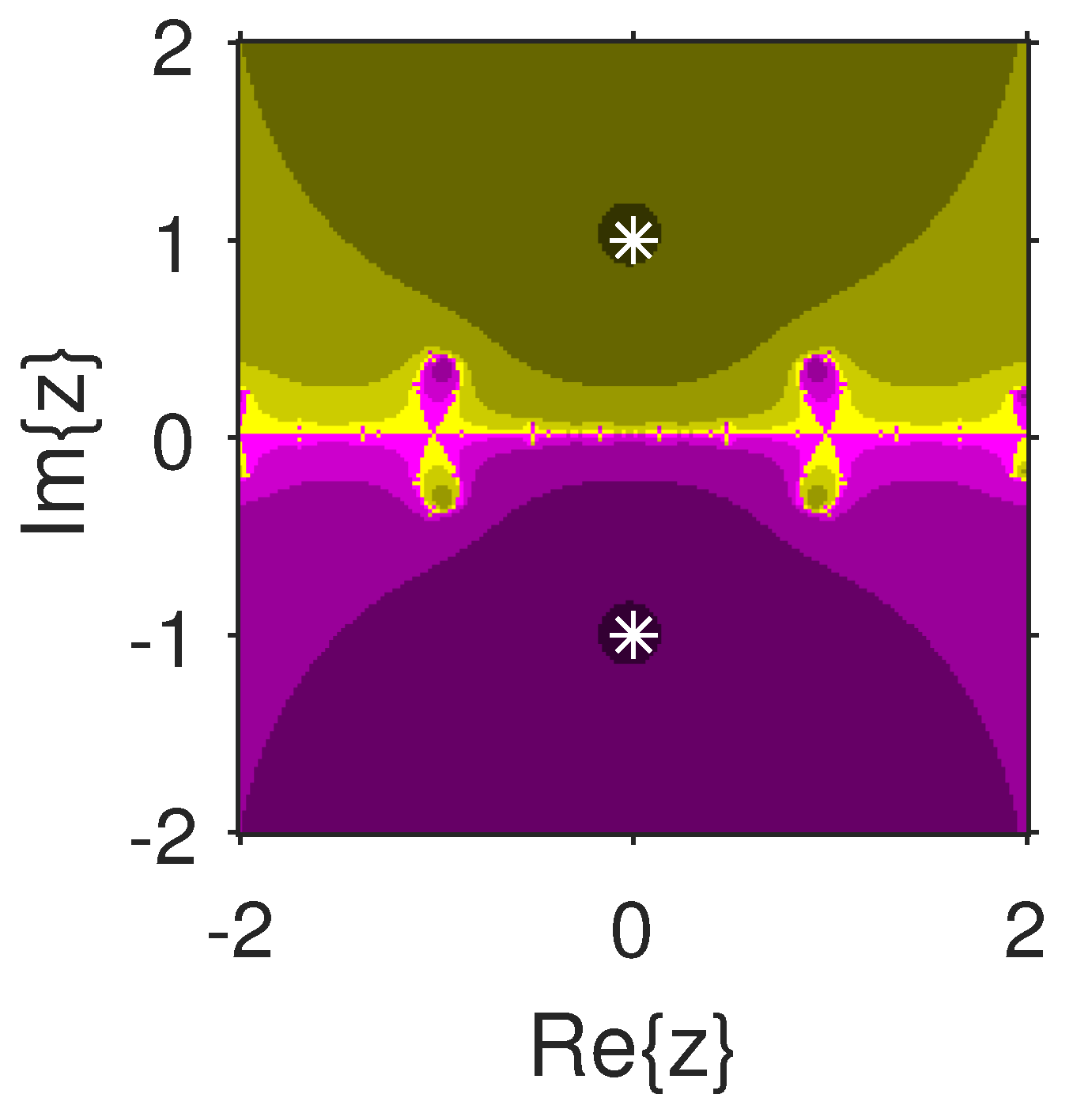
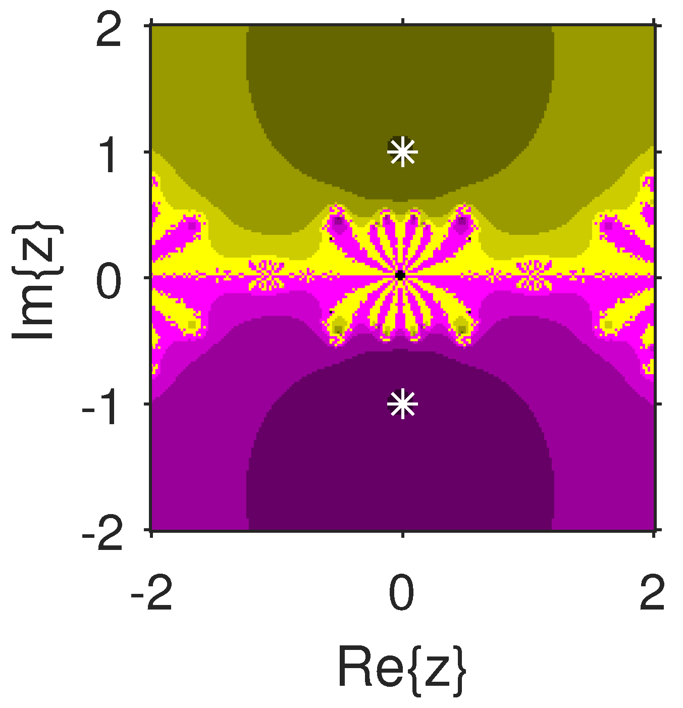
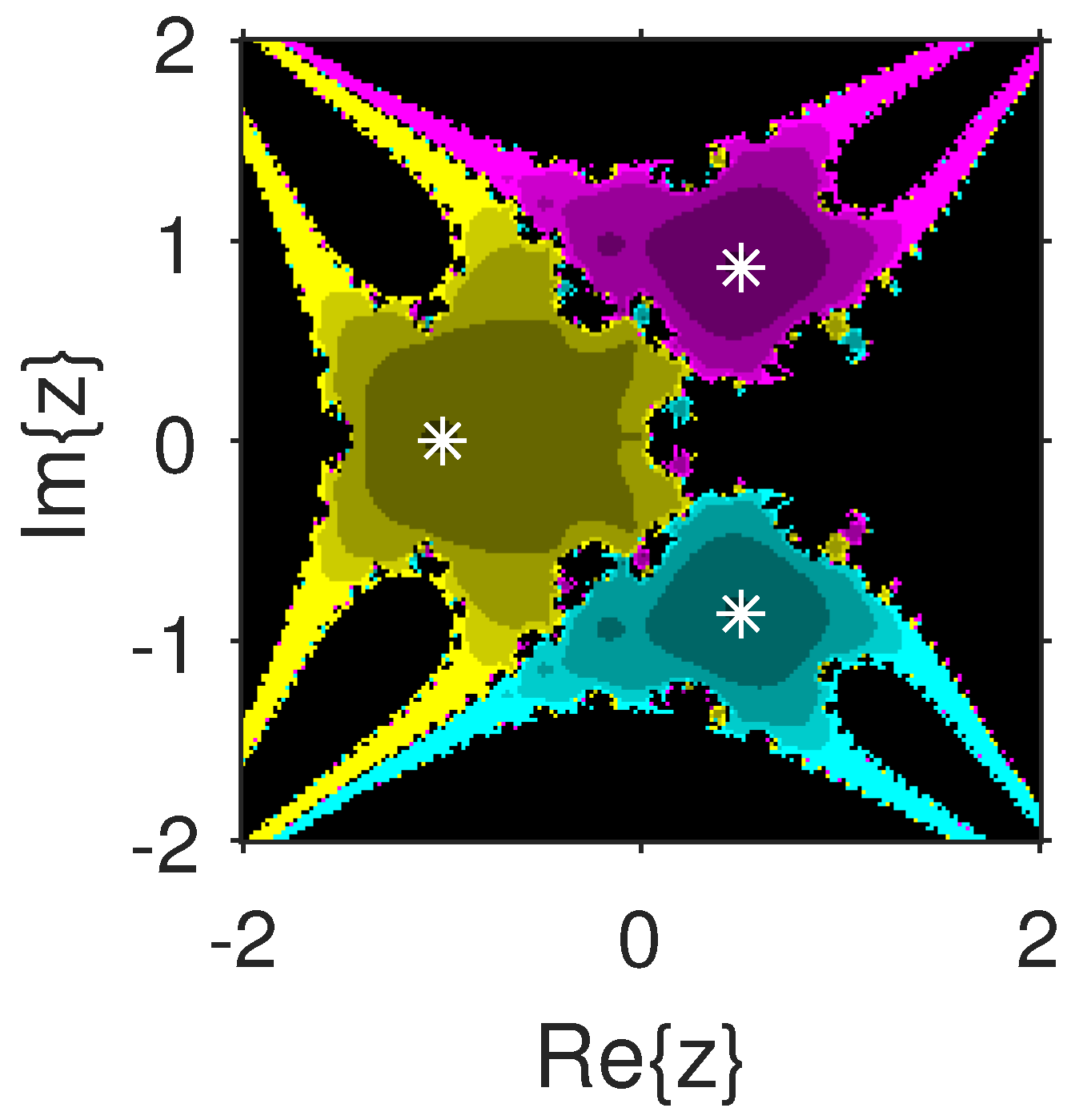
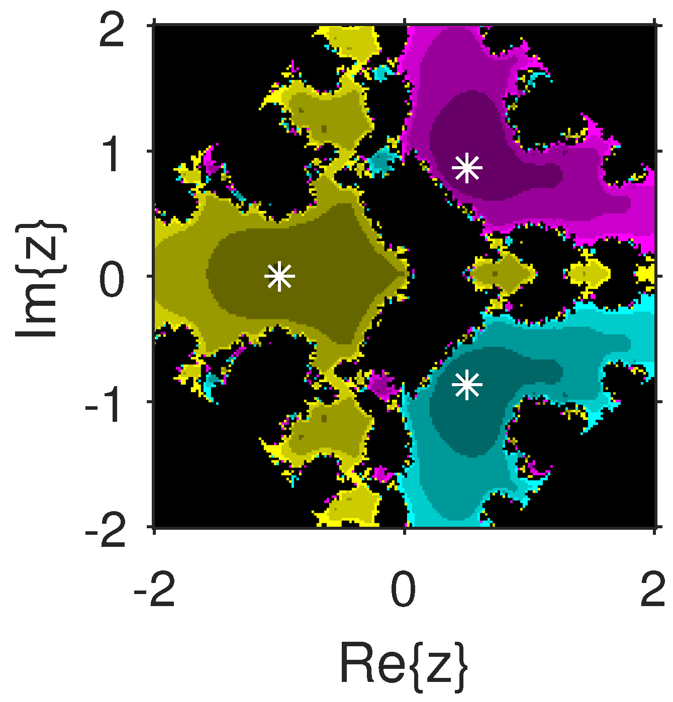
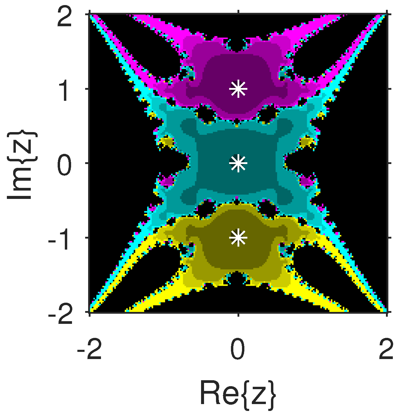
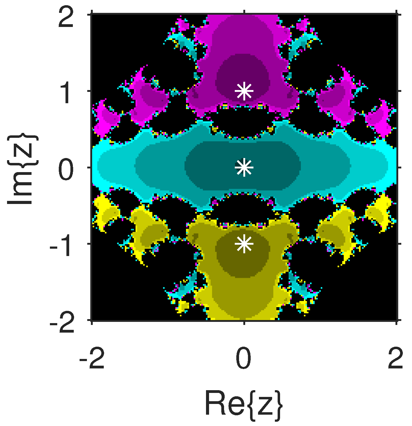
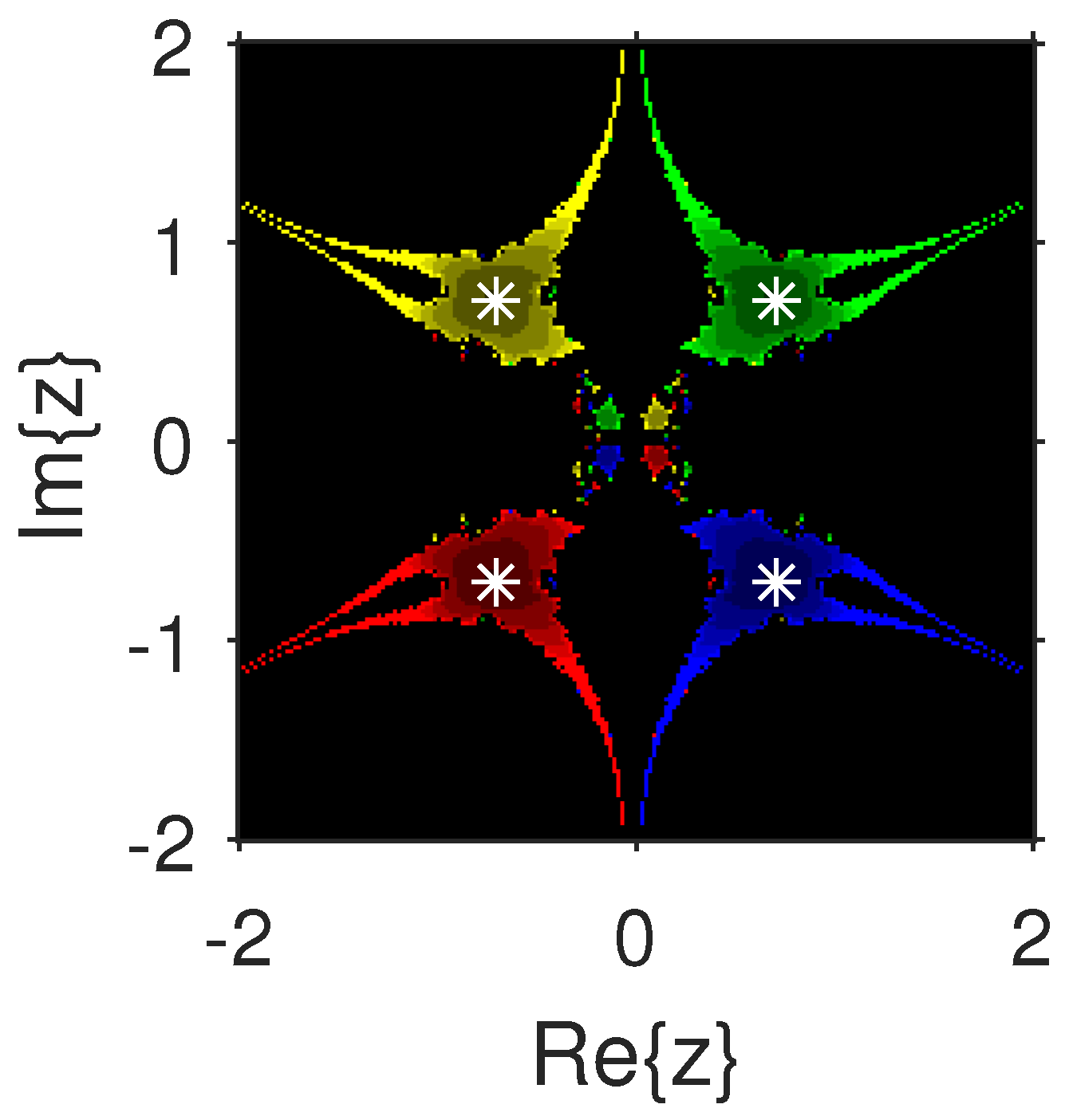
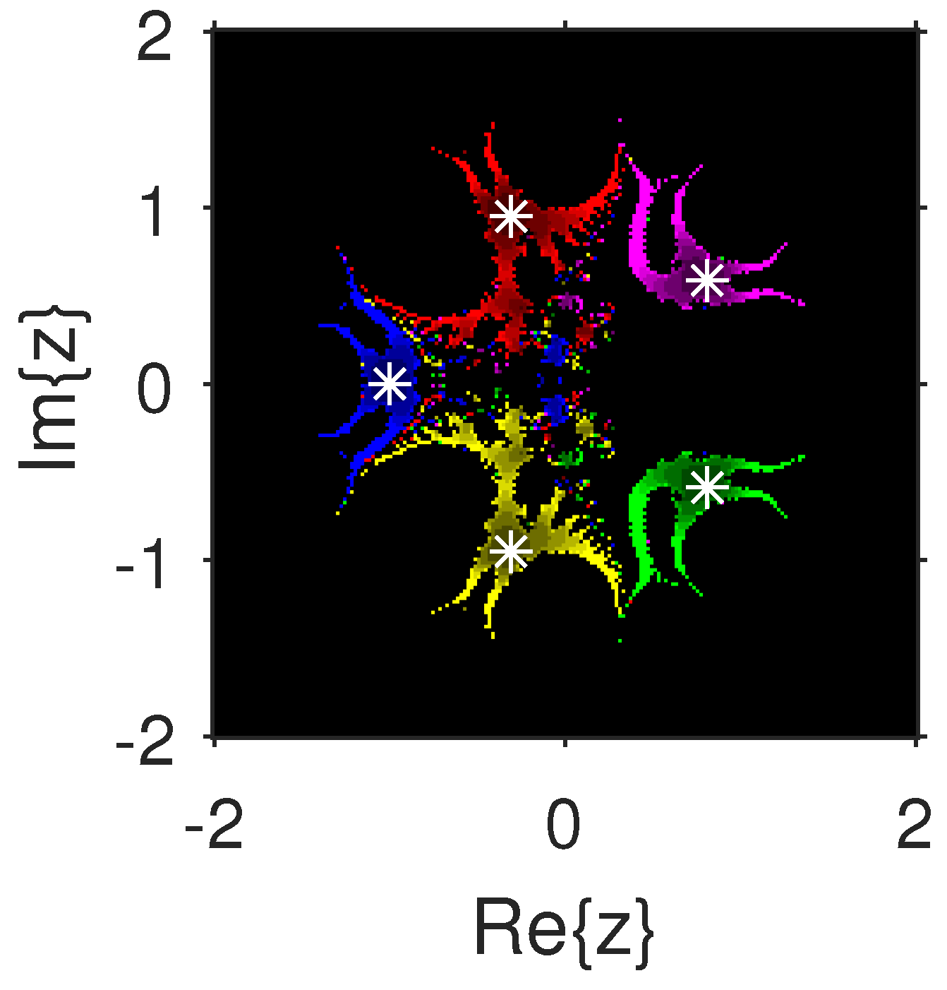
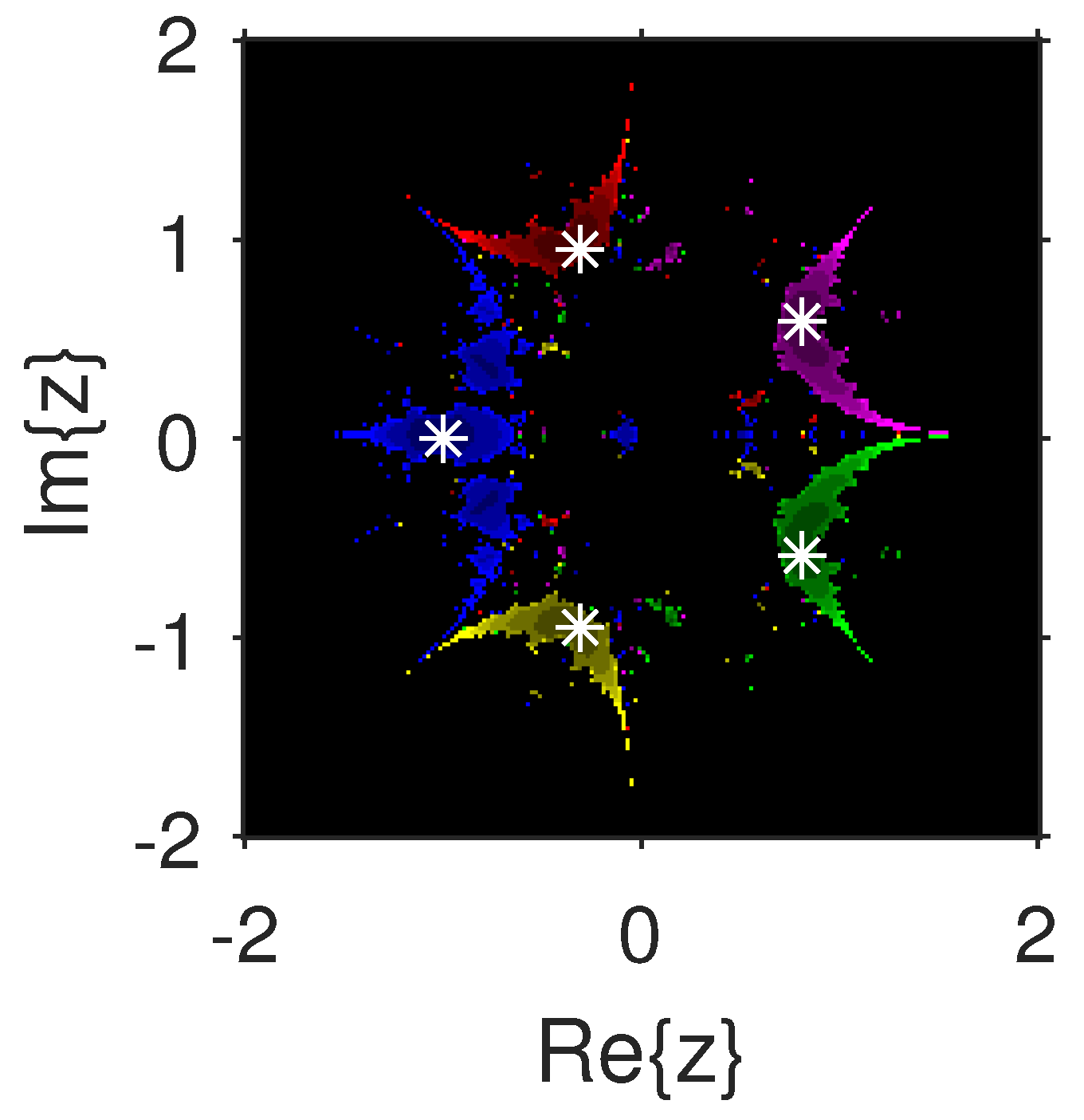
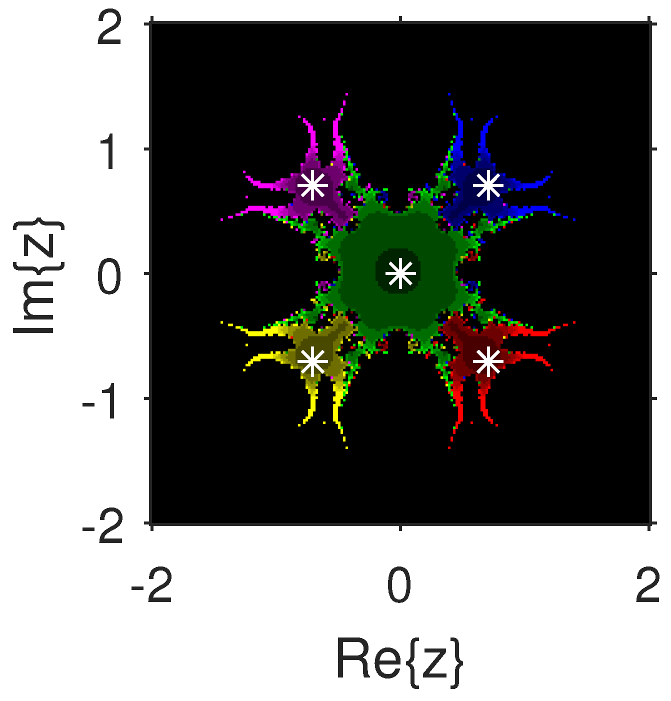
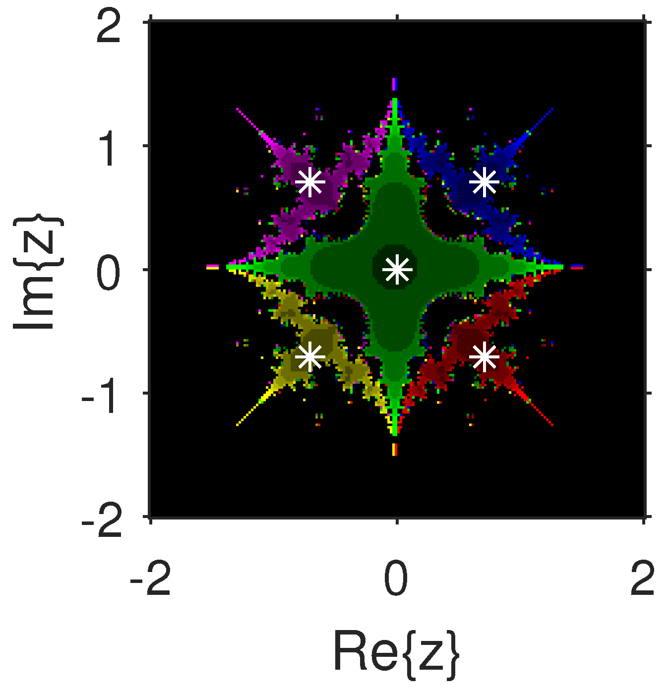
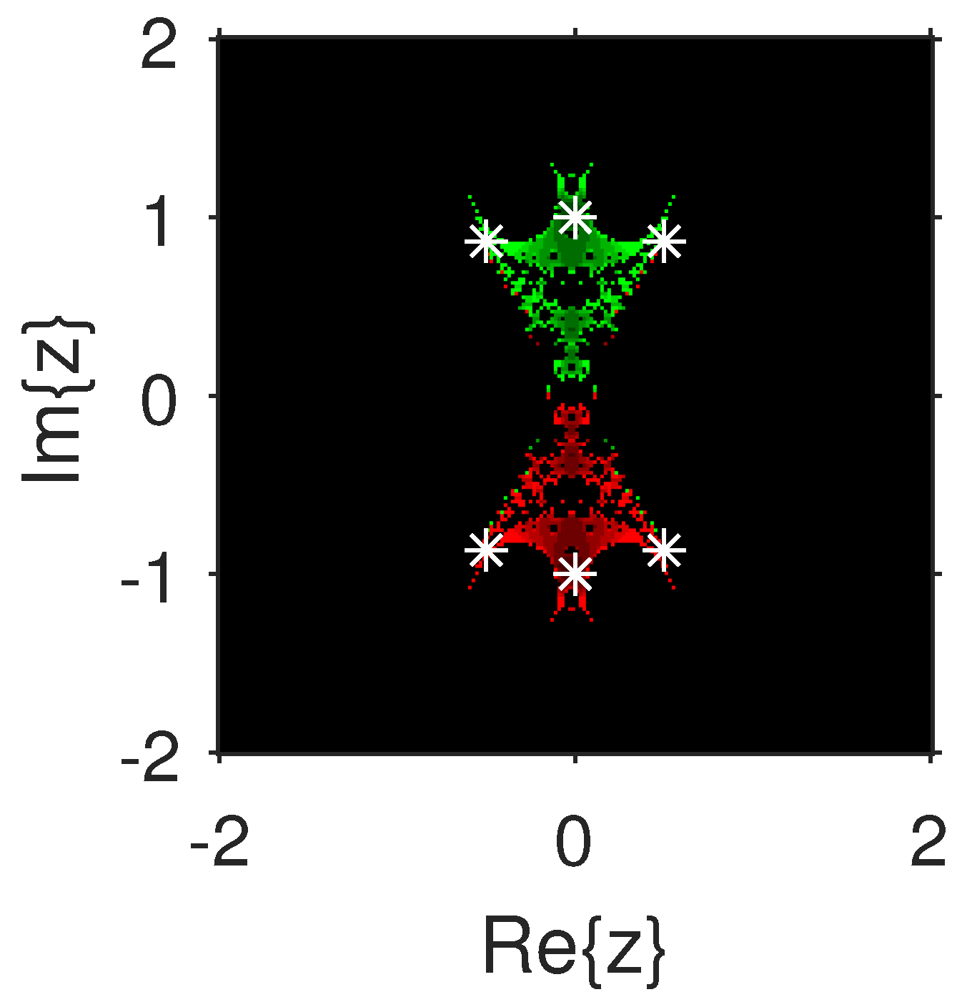
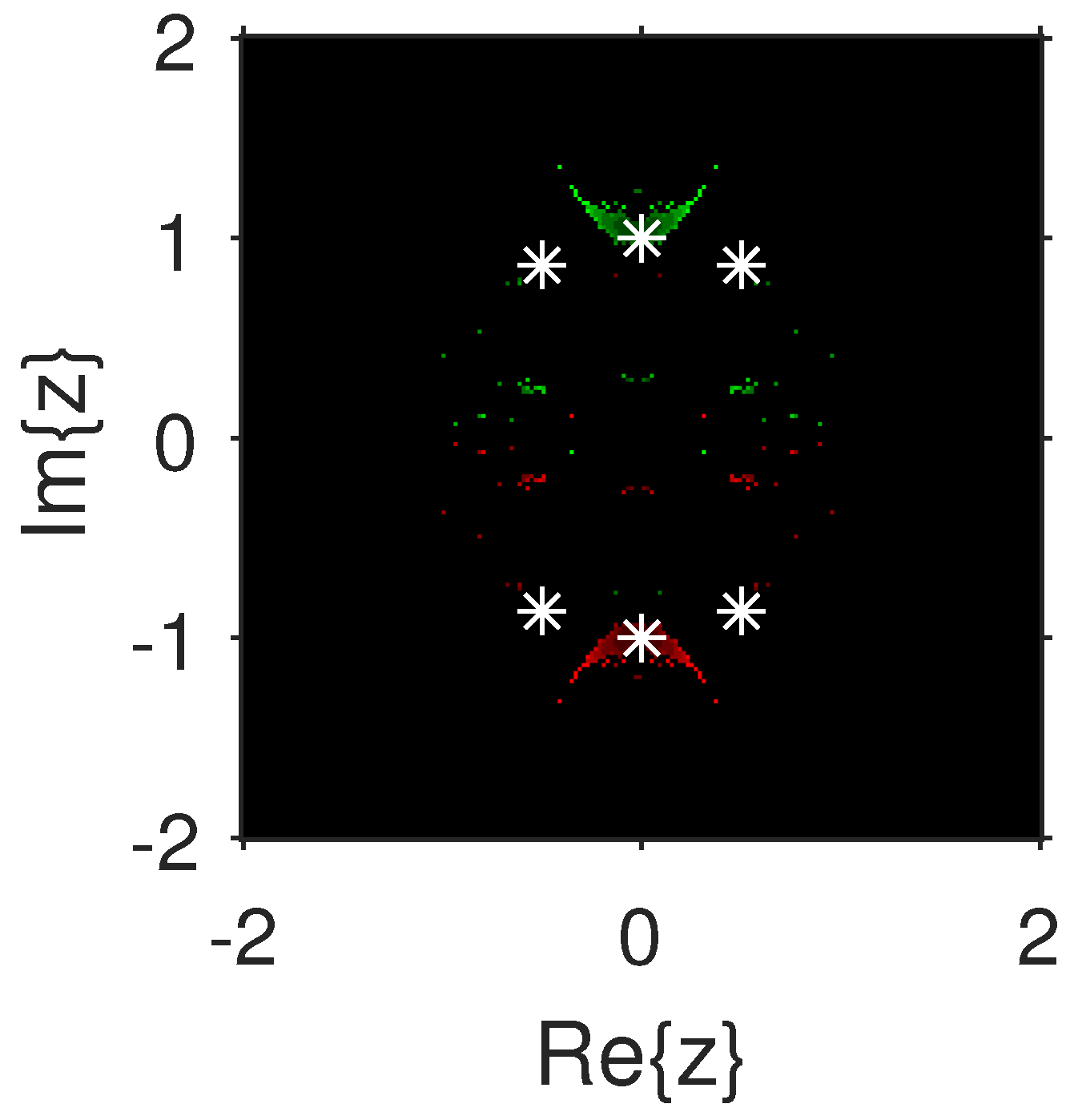
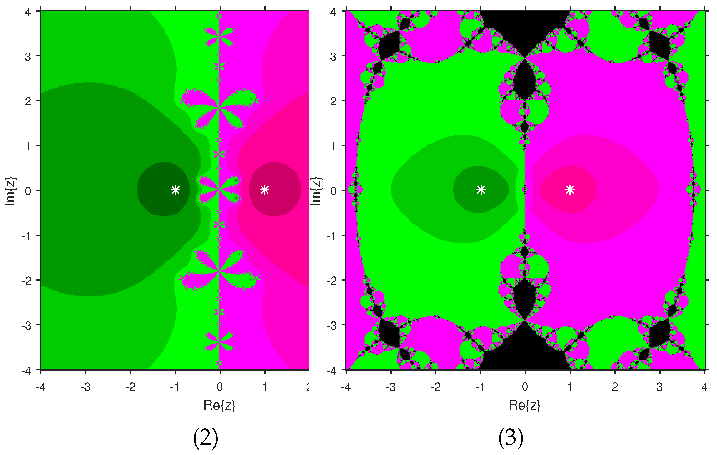
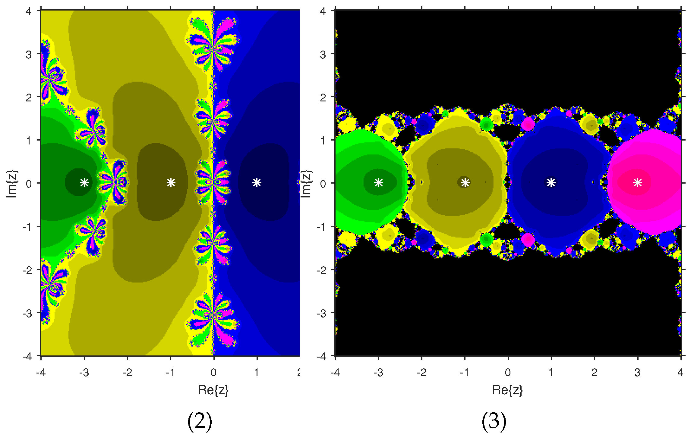
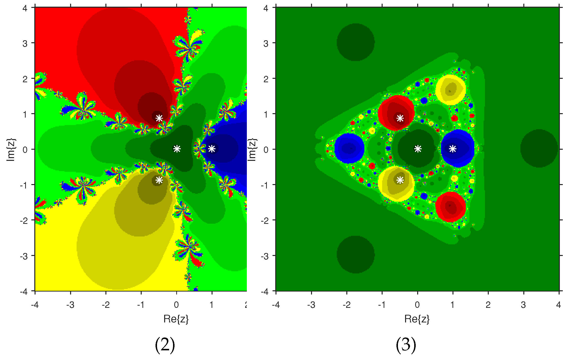
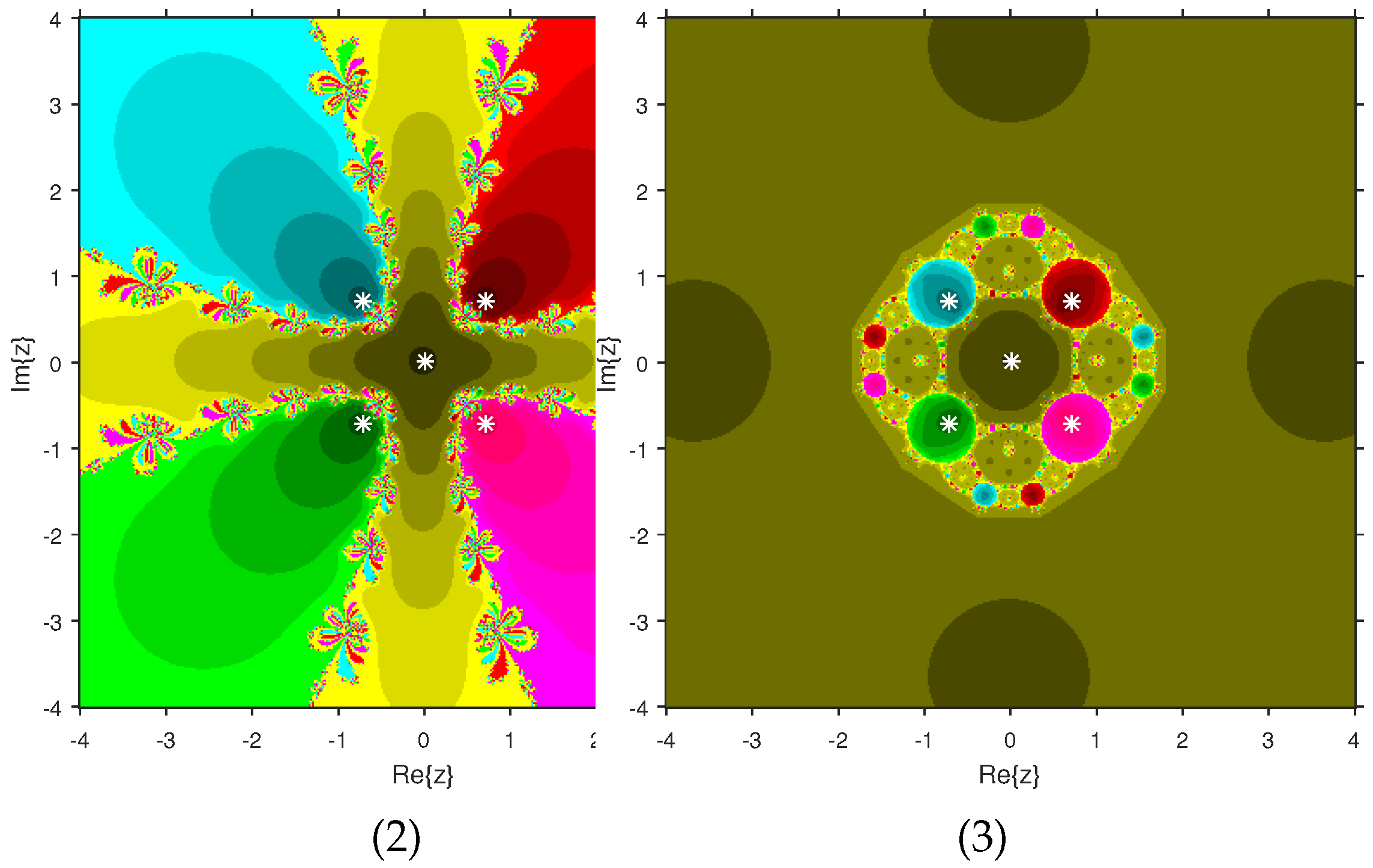
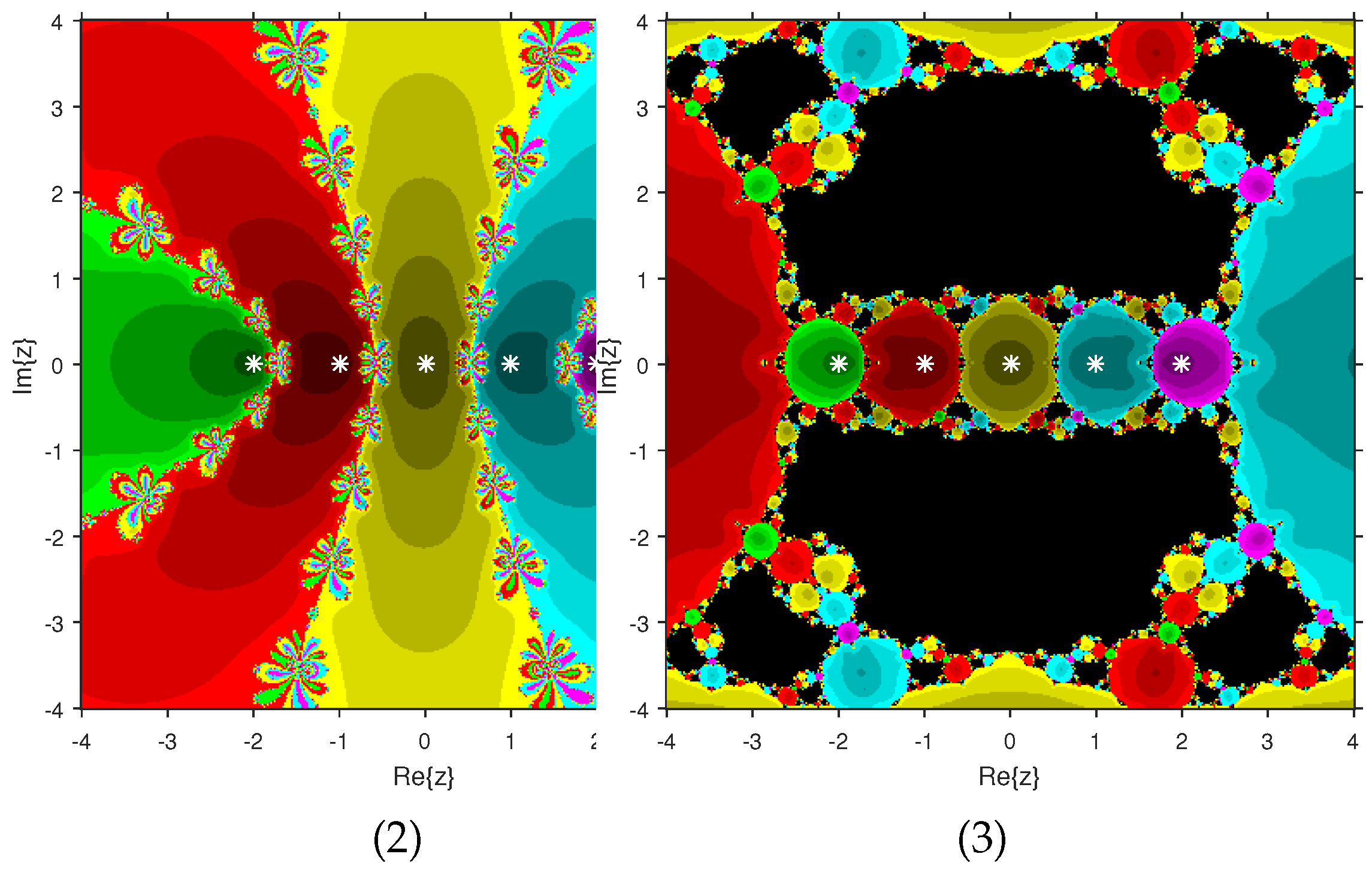
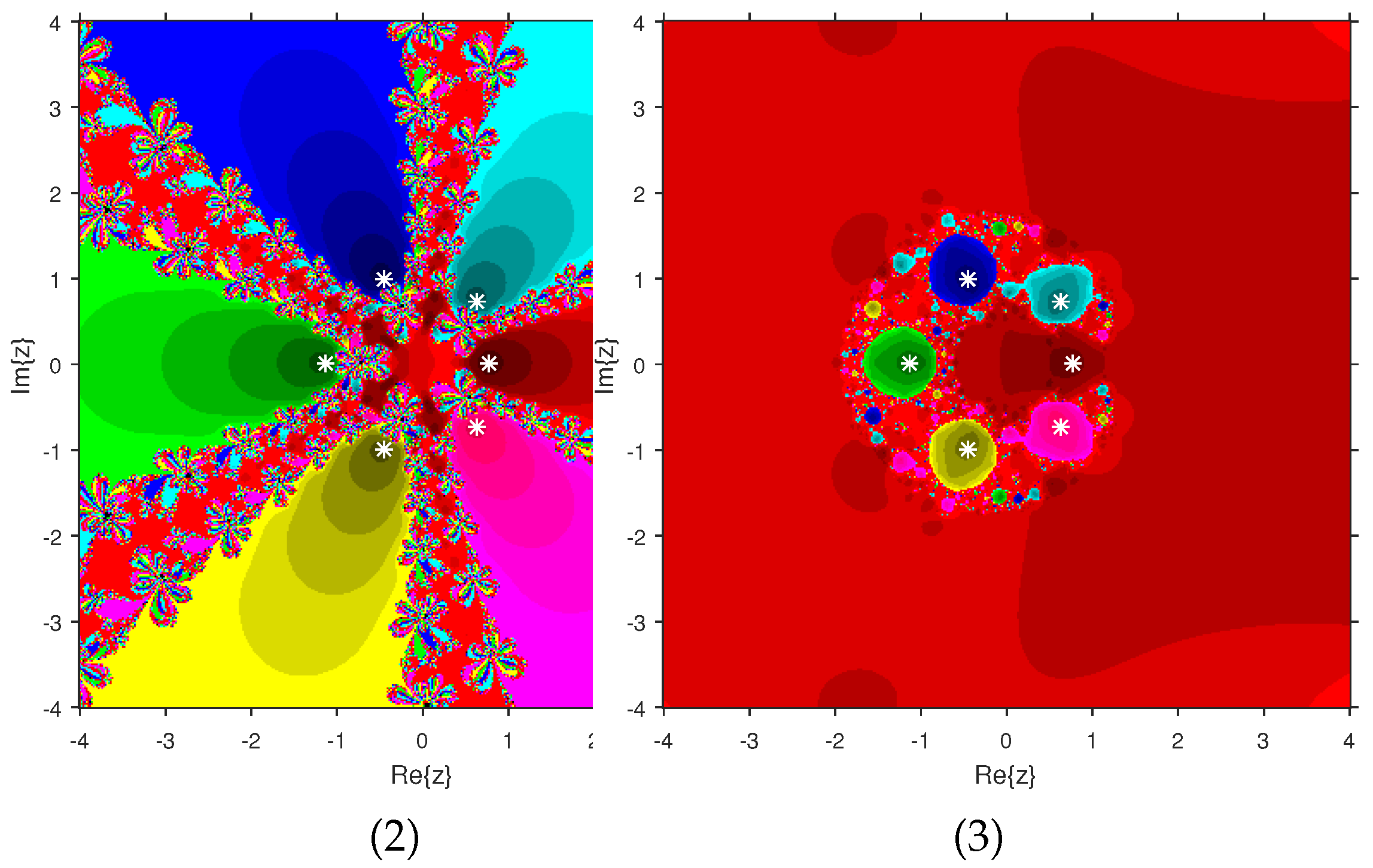
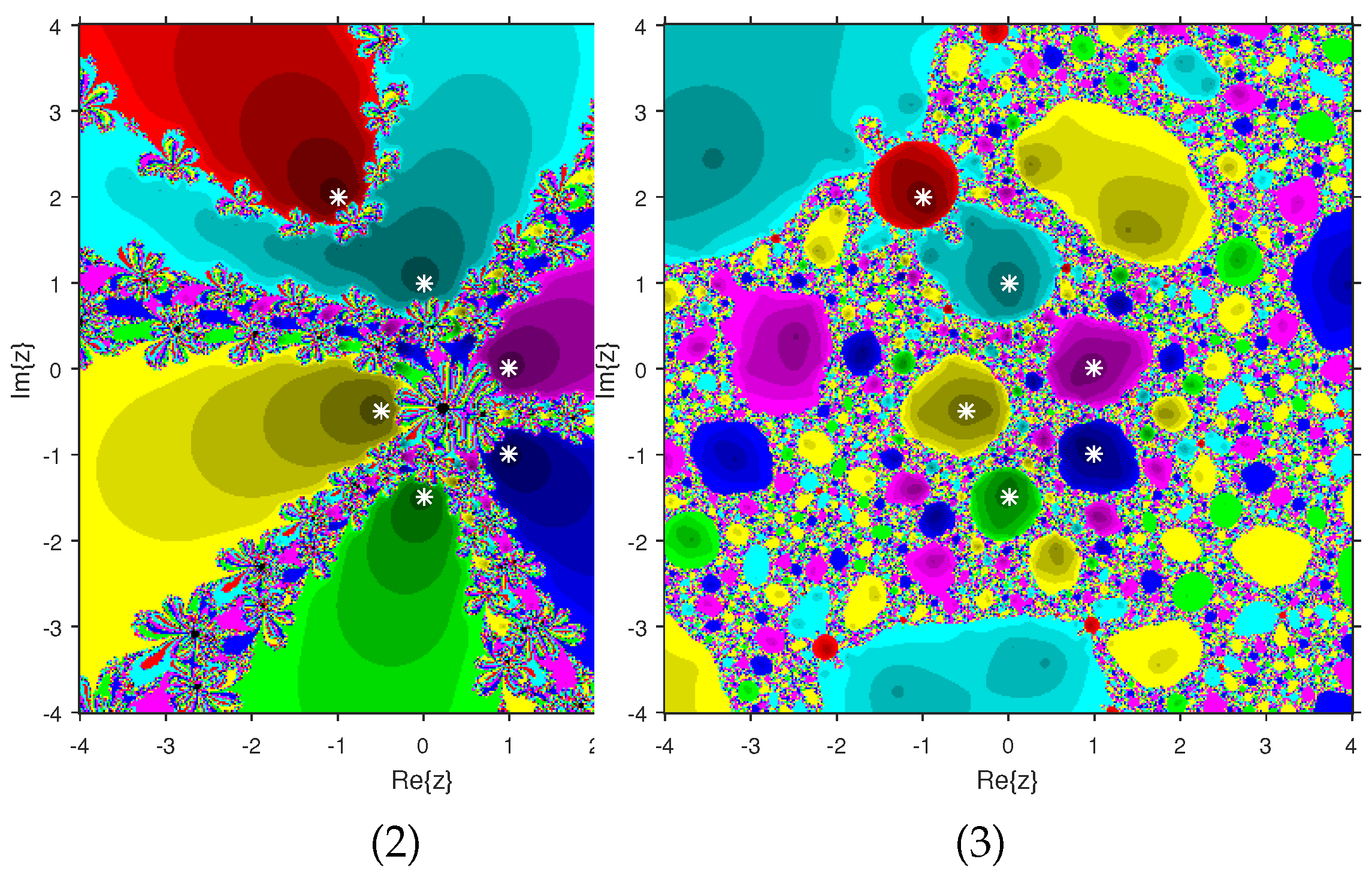
For evaluating the convergence zones of iterative algorithms the basin of attraction is a valuable geometrical tool. These basins illustrate all the initial estimations that imply convergence to a root of an equation when an iterative approach is used, allowing us to see visually which places are suitable starters and which are not. Using this excellent tool, we compare the convergence areas of $G{M}_6$ and $S{M}_6$ for a variety of complex polynomials. With the starting point $z_0\in W=[-2,2]$×$[-2,2]\subset \mathbb{C}$, $G{M}_6$ and $S{M}_6$ used on polynomials with complex coefficients. The starter $z_0$ is in the basin of a root $z_{*}$ of a test polynomial if ${\displaystyle \underset{m\to \infty }{lim}{z}_m=z_{*}}$ and then a typical color associated with $z_{*}$ is applied on $z_0$. Black color is applied on $z_0\in W$ if $\left\{z_m\right\}$ diverges. To end the iteration process, the conditions $\parallel z_m-z_{*}\parallel <{10}^{-6}$ or the maximum of 100 iterations is used. The fractal figures are created in MATLAB 2019a.

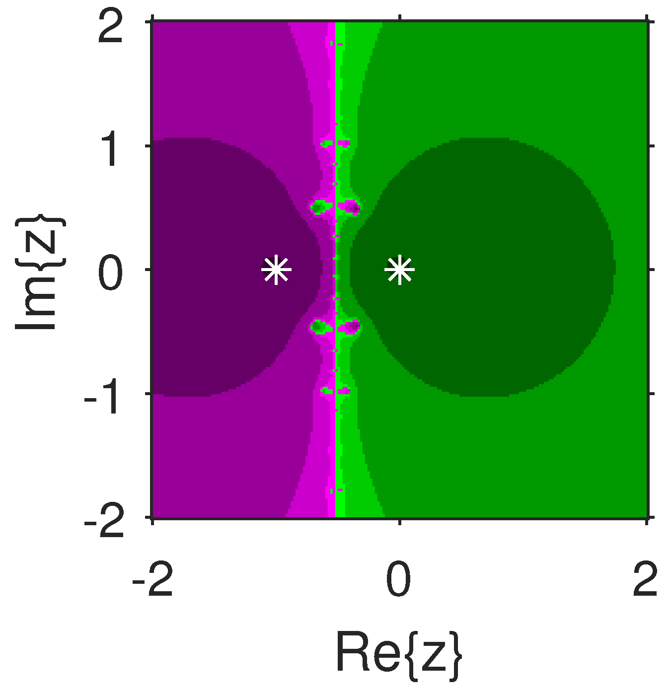
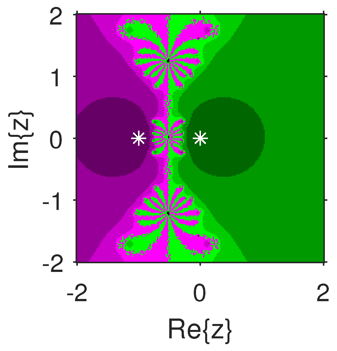
The experiment begins with the polynomials $F_1\left(z\right)=z^2+1$ and $F_2\left(z\right)=z^2+z$ to design the basins of their roots. In Figure 1 and Figure 2, yellow and magenta colors are associated with the roots i and $-i$, of $F_1\left(z\right)$, respectively. Figure 3 and Figure 4 offer basins of roots $-1$ and 0 of $F_2\left(z\right)$ in magenta and green colors, respectively. Next, the polynomials $F_3\left(z\right)=z^3+1$ and $F_4\left(z\right)=z^3+z$ are picked. 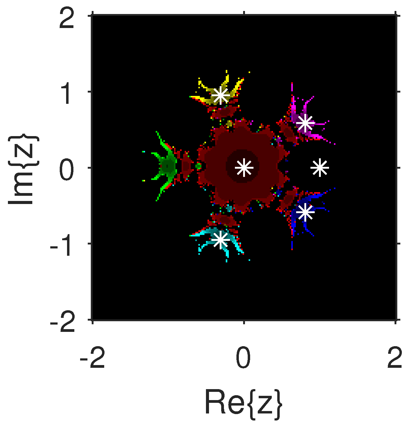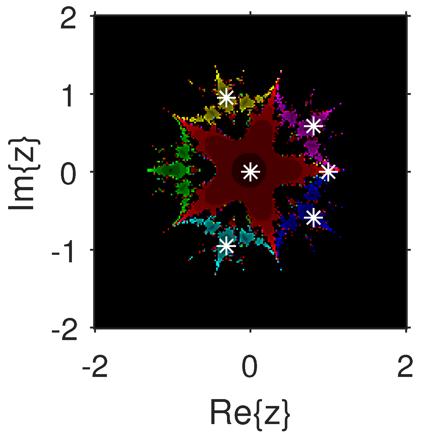Figure 5 and Figure 6 give the attraction basins of roots $\frac{1}{2}-\frac{\sqrt{3}}{2}i$, $-1$ and $\frac{1}{2}+\frac{\sqrt{3}}{2}i$ of $F_3\left(z\right)$ in cyan, yellow and magenta, respectively. In Figure 7 and Figure 8, the basins of the roots 0, $-i$, and i of $F_4\left(z\right)$ are painted in cyan, yellow and magenta colors, respectively. Further, $F_5\left(z\right)=z^4+1$ and $F_6\left(z\right)=z^4+z$ are chosen to decorate the attraction basins of their roots. 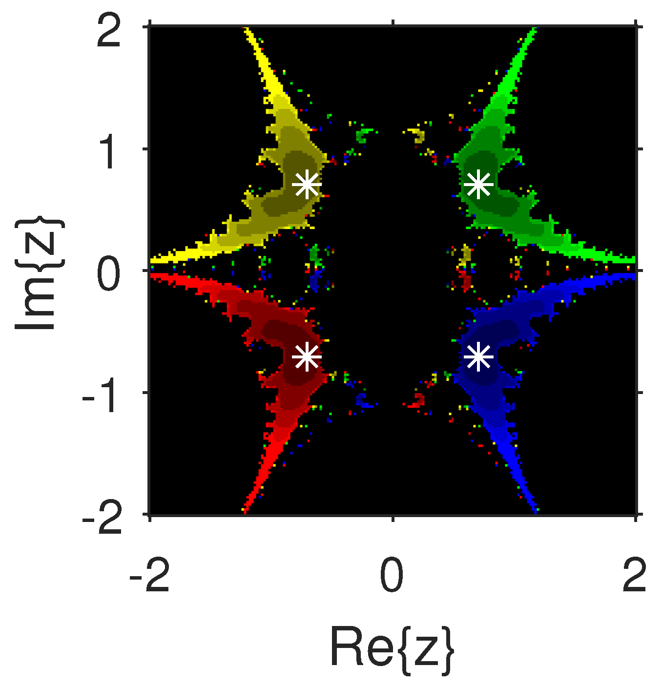In Figure 9 and Figure 10, the basins of the roots $0.707106+0.707106i$, $0.707106-0.707106i$, $-0.707106-0.707106i$ and $-0.707106+0.707106i$ of $F_5\left(z\right)=0$ are, respectively, indicated in green, blue, red and yellow zones. In Figure 11 and Figure 12, convergence to the roots $-1$, $\frac{1}{2}+\frac{\sqrt{3}}{2}i$, $\frac{1}{2}-\frac{\sqrt{3}}{2}i$ and 0 of the polynomial $F_6\left(z\right)$ is presented in yellow, blue, green and red, respectively. Furthermore, $F_7\left(z\right)=z^5+1$ and $F_8\left(z\right)=z^5+z$ are taken. In Figure 13 and Figure 14, magenta, green, yellow, blue and red colors are applied to the basins of roots $0.809016+0.587785i$, $0.809016-0.587785i$, $-0.309016-0.951056i$, $-1$ and $-0.309016+0.951056i$, respectively, of $F_7\left(z\right)$. 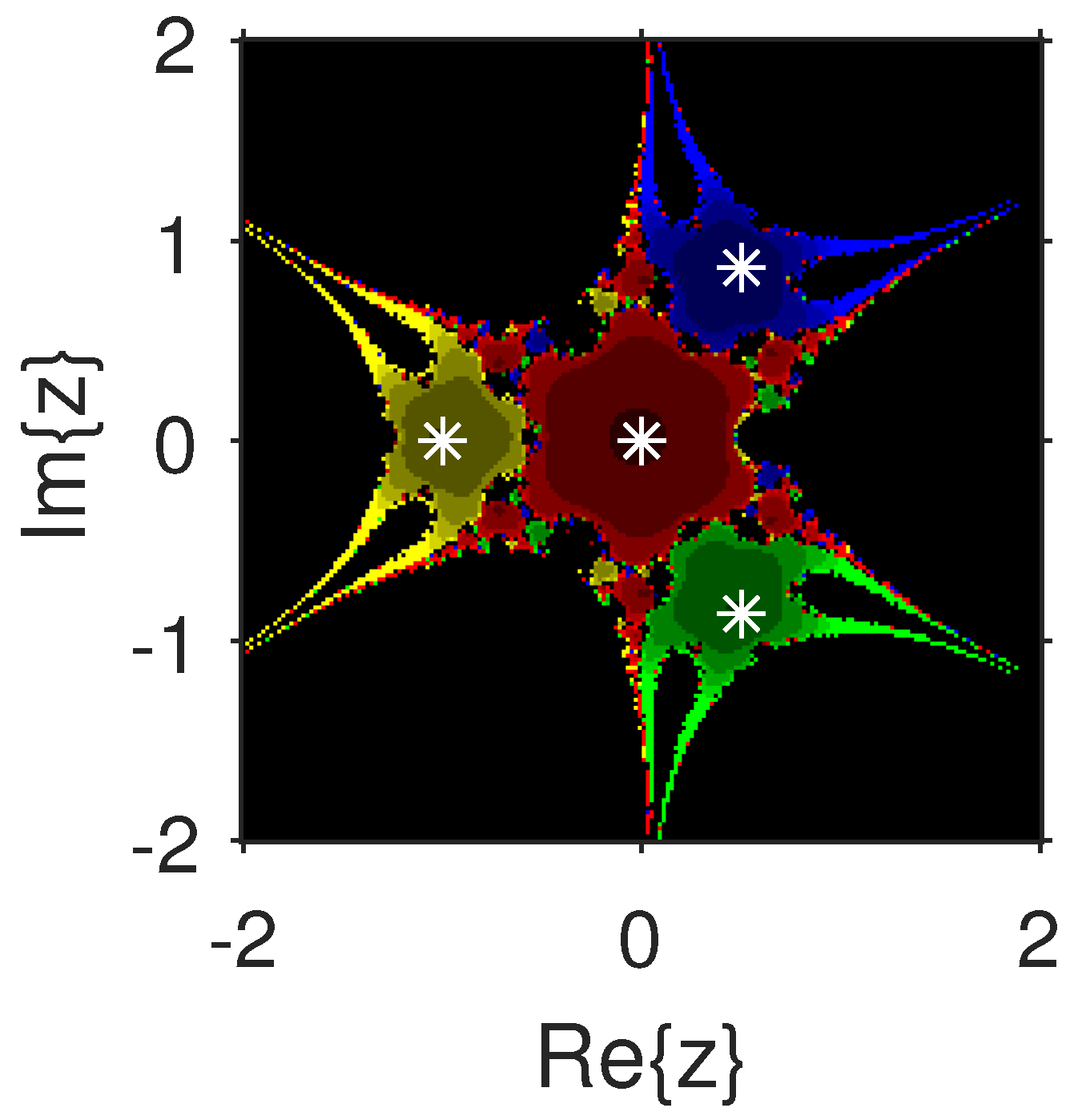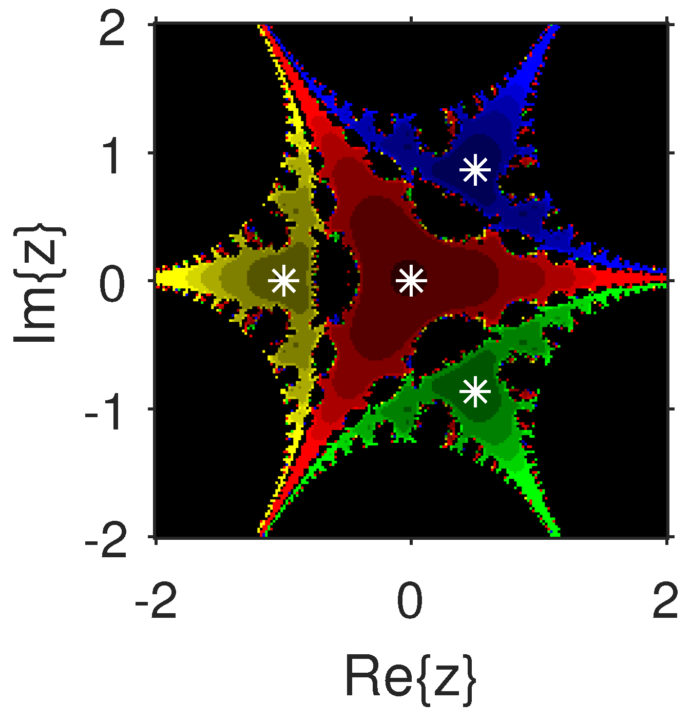Figure 15 and Figure 16 display the basins of the roots $0.707106+0.707106i$, 0, $-0.707106+0.707106i$, $-0.707106-0.707106i$ and $0.707106-0.707106i$ of $F_8\left(z\right)=0$ in blue, green, magenta, yellow, and red colors, respectively. Lastly, we select $F_9\left(z\right)=z^6+1$ and $F_{10}\left(z\right)=z^6+z$. In Figure 17 and Figure 18, the basins of the roots $0.500000-0.866025i$, $0.500000+0.866025i$, $1i$, $-0.500000-0.866025i$, $-0.500000+0.866025i$ and $-1i$ of $F_9\left(z\right)=0$ are illustrated in yellow, blue, green, magenta, cyan and red, respectively. Figure 19 and Figure 20 give the basins of the roots $-1$, $-0.3090169+0.951056i$, 0, $-0.3090169-0.951056i$, $0.809016+0.587785i$ and $0.809016-0.587785i$ of $F_{10}\left(z\right)=0$ in green, yellow, red, cyan, magenta and blue colors, respectively.

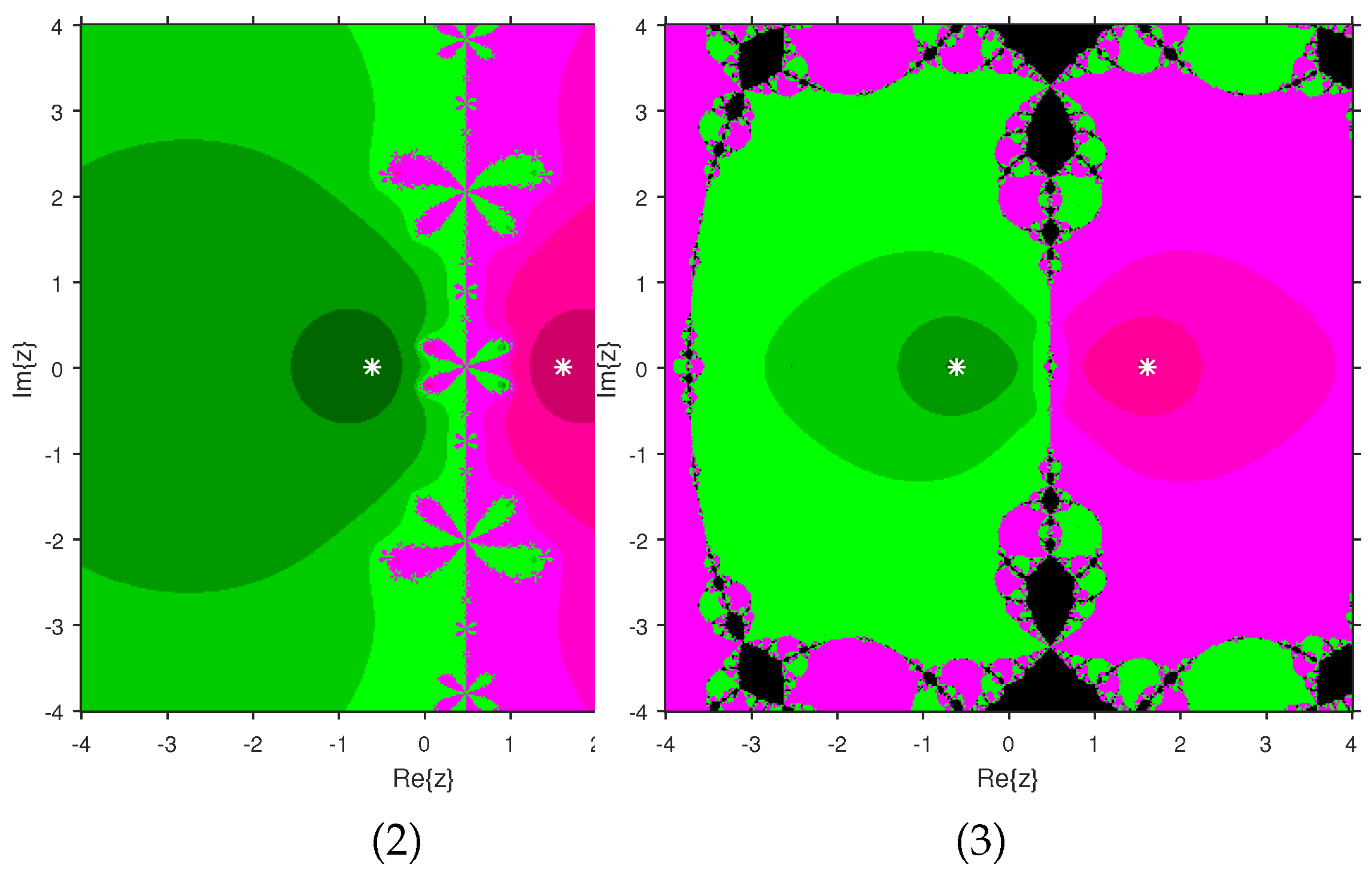
We consider polynomials $W_1\left(z\right)=z^2-1$ and $W_2\left(z\right)=z^2-z-1$ of degree two. The results of the comparison between attraction basins for (2) and (3) are displayed in Figure 21 and Figure 22. In Figure 21, green and pink areas show the attraction basins corresponding to the roots $-1$ and 1, respectively, of $W_1\left(z\right)$. The basins of the roots $\frac{1+\sqrt{5}}{2}$ and $\frac{1-\sqrt{5}}{2}$ of $W_2\left(z\right)=0$ are shown in Figure 22 by using pink and green colors, respectively. 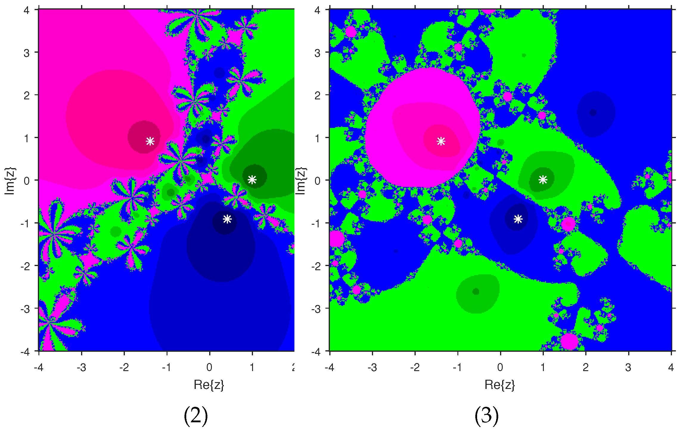Figure 23 and Figure 24 determine the attraction basins for (2) and (3) associated with the roots of $W_3\left(z\right)=z^3+(-0.7250+1.6500i)z-0.2750-1.6500i$ and $W_4\left(z\right)=z^3-z$. The basins for (2) and (3) associated with the roots 1, $-1.401440+0.915201i$ and $0.4014403-0.915201i$ of $W_3\left(z\right)$ are given in Figure 23 by means of green, pink and blue domains, respectively. 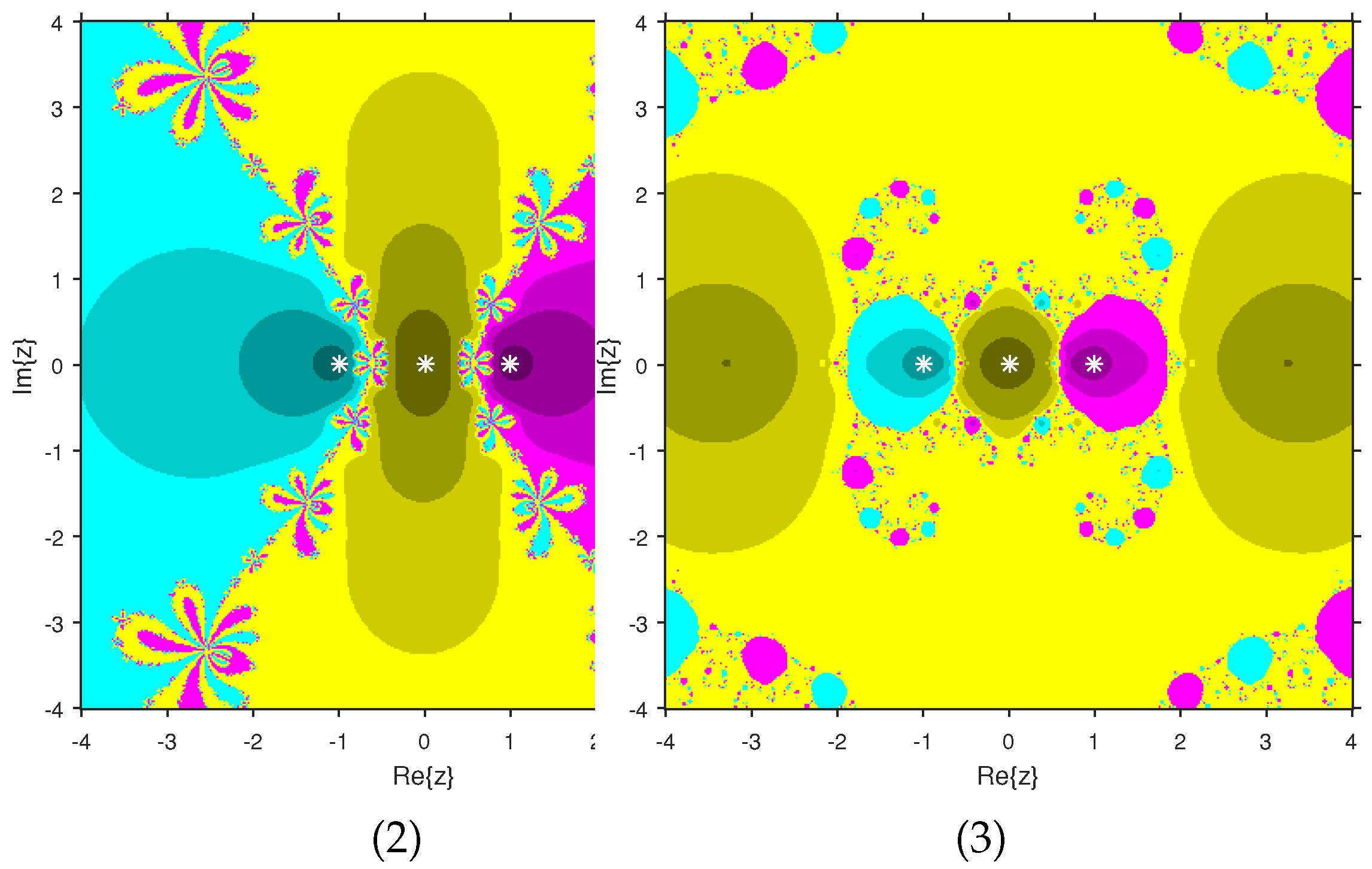In Figure 24, the basins of the roots 0, 1, and $-1$ of $W_4\left(z\right)=0$ are painted in yellow, magenta and cyan, respectively. Next, we use polynomials $W_5\left(z\right)=z^4-10z^2+9$ and $W_6\left(z\right)=z^4-z$ of degree four to compare the attraction basins for (2) and (3). The basins for (2) and (3) corresponding to the roots $-1$, 3, $-3$ and 1 of $W_5\left(z\right)$ are illustrated in Figure 25 using yellow, pink, green and blue colors, respectively. Figure 26 gives the comparison of basins for these schemes associated with the roots 0, 1, $-\frac{1}{2}-\frac{3}{2}i$ and $-\frac{1}{2}+\frac{3}{2}i$ of $W_6\left(z\right)=0$, which are denoted in green, blue, yellow and red regions, respectively. Moreover, we select polynomials $W_7\left(z\right)=z^5+z$ and $W_8\left(z\right)=z^5-5z^3+4z$ of degree five to give and compare the attraction basins for (2) and (3). In Figure 27, green, cyan, red, pink and yellow regions illustrate the attraction basins of the roots $-0.707106-0.707106i$, $-0.707106+0.707106i$, $0.707106+0.707106i$, $0.707106-0.707106i$ and 0, respectively, of $W_7\left(z\right)=0$. Figure 28 gives the basins of roots 0, 2, $-1$, $-2$ and 1 of $W_8\left(z\right)$ in yellow, magenta, red, green and cyan colors, respectively. Lastly, sixth degree complex polynomials $W_9\left(z\right)=z^6+z-1$ and $W_{10}\left(z\right)=z^6-0.5z^5+\frac{11}{4}(1+i)z^4-\frac{1}{4}(19+3i)z^3+\frac{1}{4}(11+i)z^2-\frac{1}{4}(19+3i)z+\frac{3}{2}-3i$ are considered. In Figure 29, green, pink, red, yellow, cyan and blue colors are used to give the basins related to the roots $-1.134724$, $0.629372-0.735755i$, $0.7780895$, $-0.451055-1.002364i$, $0.629372+0.735755i$ and $-0.451055+1.002364i$ of $W_9\left(z\right)=0$, respectively. In Figure 30, the attraction basins for (2) and (3) corresponding to the roots $1-i$, $-\frac{1}{2}-\frac{i}{2}$, $-\frac{3}{2}i$, 1, i and $-1+2i$ of $W_{10}\left(z\right)$ are provided in blue, yellow, green, magenta, cyan and red colors, respectively.

From Figure 21, Figure 22, Figure 23, Figure 24, Figure 25, Figure 26, Figure 27, Figure 28, Figure 29 and Figure 30, we deduce that (2) has the wider basins in comparison to (3). as it can be seen that the black zones that appear in Figure 21, Figure 25 and Figure 28 only appear in (3) method and not in (2). Furthermore, (2) is better than (3) in terms of less chaotic behavior as it can be seen that basins are bigger in (2) and there are fewer changes of basin than in (3) in each figure, which means that the fractal dimension is lower in (2) and consequently less chaotic. Hence, the overall conclusion of this comparison is that the numerical stability of (2) is higher than (3). This means that (2) is the preferable alternative for solving real problems. Moreover, related to the patterns that appear in the basin of attraction, it is clear that the (2) is similar to third-order methods such us Halley or Chebyshev and the immediate basin of attraction is big and black zones are avoided. On the other hand, in the (3) everything seems more independent with different structures, for example in Figure 29 where the roots are bounded by a small basin and then a really big one in red appears or Figure 21, Figure 25 and Figure 28 where zones with no convergence appear, especially in Figure 25 where almost the half of the plane is black. Finally, in Figure 24, Figure 26, Figure 27, and Figure 29 it seems that a compactification appears in the roots but one of the basins is much bigger than the rest, and this behavior is really interesting and can be considered in the future.

4. Examples

The convergence radii are determined for the iterative procedures $G{M}_6$ and $S{M}_6$.

Example 1.

Let $T_1=T_2={\mathbb{R}}^3$ and $A=\overline{D}(0,1)$. Consider L on A for $t={(t_1,t_2,t_3)}^T$ as

$$L\left(t\right)={(e^{t_1}-1,\frac{e-1}{2}{t}_2^2+t_2,t_3)}^T$$

Notice that

$$t_{*}=\left[\begin{array}{c}0\\ 0\\ 0\end{array}\right]$$

Also,

$$\begin{array}{cc}\hfill a=b& =\frac{1}{2}(3+e^{\frac{1}{e-1}}),c=2,\hfill \\ \hfill B_0(v,v_1)& =\frac{(e-1)}{2}(v+v_1),\hfill \\ \hfill B(v,v_1)& =\frac{e^{\frac{1}{e-1}}}{2}(v+v_1),\hfill \\ \hfill B_1(v,v_1)& =\frac{1}{2}(e^{\frac{1}{e-1}}v+(e-1)v_1).\hfill \end{array}$$

Using proposed theorems, we obtained r and $\overline{r}$. These radii are given in

Table 1. Comparison of the radii in Example 1.

${\mathit{SM}}_6$	${\mathit{GM}}_6$
$r_1=0.124265$	$r_1=0.124265$
$\overline{r_2}=0.071733$	$r_2=0.064445$
$\overline{r_3}=0.057472$	$r_3=0.052507$
$\overline{r}=0.057472$	$r=0.052507$

.

Example 2.

Let us choose $T_1=T_2=C[0,1]$ and $A=\overline{D}(0,1)$. Consider the operator L on A defined as

$$L\left(t\right)\left(v\right)=t\left(v\right)-5{\int }_0^{1}vs.yt{\left(y\right)}^{3}dy,$$

where $t\left(v\right)\in C[0,1]$. We have $t_{*}=0$. Furthermore,

$$\begin{array}{cc}\hfill a=b& =9,c=2,\hfill \\ \hfill B_0(x,y)& =\frac{7.5}{2}(x+y),\hfill \\ \hfill B(x,y)& =\frac{15}{2}(x+y),\hfill \\ \hfill B_1(x,y)& =\frac{1}{2}(15x+7.5y).\hfill \end{array}$$

The convergence radii r and $\overline{r}$ are obtained using the suggested theorems and presented in

Table 2. Comparison of the radii in Example 2.

${\mathit{SM}}_6$	${\mathit{GM}}_6$
$r_1=0.066667$	$r_1=0.066667$
$\overline{r_2}=0.004614$	$r_2=0.003524$
$\overline{r_3}=0.003497$	$r_3=0.002828$
$\overline{r}=0.003497$	$r=0.002828$

.

Example 3.

We solve the nonlinear systems

$$\begin{array}{cc}\hfill y_m{y}_{m+1}-1& =0,1\le m\le 18\hfill \\ \hfill y_m{y}_1-1& =0,m=19.\hfill \end{array}$$

The initial point is chosen to be $t_0={[1.5,1.5,\cdots ,1.5]}^T$. Then, the two-step method (2) and (3) after three iterations as well as the three-step methods (2) and (3) after two iterations given the solution vector $t_{*}={[1,1,\cdots ,1]}^T$.

Example 4.

Let us consider the two-point differential equation

$$w^{″}+3w{w}^{\prime }=0,w\left(0\right)=0,w\left(2\right)=1.$$

Moreover, let

$$p_0=0<p_1<p_2\cdots <p_{j-1}<p_j=2,p_{i+1}=p_i+h,h=\frac{2}{i}.$$

Set $p_0=w\left(p_0\right)=0$, $p_1=w\left(p_1\right)=\cdots =p_{i-1}=w\left(p_{i-1}\right)$ and $p_i=w\left(p_i\right)=1$.

The central difference for first, as well as the second order derivative discretion, give

$$\begin{array}{cc}\hfill w_i^{″}& =\frac{w_{i-1}-2w_i+w_{i+1}}{h^2},i=1,2,\cdots ,j-1\hfill \\ \hfill w_i^{\prime }& =\frac{w_{i+1}-w_{i-1}}{h^2},i=1,2,\cdots ,j-1\hfill \\ \hfill w_i& =\frac{w_{i+1}+w_{i-1}}{2},i=1,2,\cdots ,j-1.\hfill \end{array}$$

By these substitutions, we obtain that $(j-1)(j-1)$ nonlinear system.

$$4(w_{i-1}-2w_i+w_{i+1})+3h(w_{i+1}^2-w_{i-1}^2)=0,i=1,2,\cdots ,j-1.$$

This system is solved for $j=6$. Let $t_0={[0.5,0.5,0.5,0.5,0.5]}^T$. Then, if we apply the two-step methods (2) and (3) after three iterations or the three-step methods (2) and (3) after two iterations we obtain the solution vector $t_{*}$ with five entries given by

$$t_{*}={[0.4524453796,0.760355997,0.9116610553,0.9715327158,0.9927818807]}^T.$$

5. Conclusions

A comparison is made between the convergence balls and dynamical behaviors of two derivative free equation solvers that are similar in their efficiency. The ball convergence of $G{M}_6$ and $S{M}_6$ solely require generalized Lipschitz continuity of $L^{\prime }$. Then, the convergence zones of $G{M}_6$ and $S{M}_6$ are presented using the geometric tool attraction basins. Finally, our analytical conclusions are validated against real-world application challenges. The scheme $S{M}_6$ is discovered to have bigger convergence balls than the solver $G{M}_6$. Future research will involve the extension of this technique to multipoint method [1,4].