


Stability Analysis of Fractional-Order Mathieu Equation with Forced Excitation


Abstract
:1. Introduction
2. Stability Analysis of Fractional-Order Parametrically Excited System
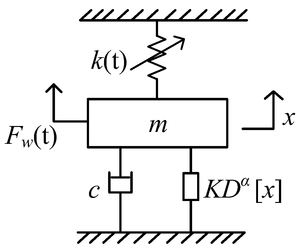
2.1. The Fractional-Order Model of the Pantograph–Catenary System
2.2. Extended Floquet Theory
- If , , then , and the properties of the solution satisfy the asymptotic stability.
- If , , then , and the properties of the solution satisfy the instability.
- If , , then the solution is stable without the interference of forced excitation, and when there exists a positive integer m, also satisfying , we can obtain the solutions with k’T-periodic.
- 3.1
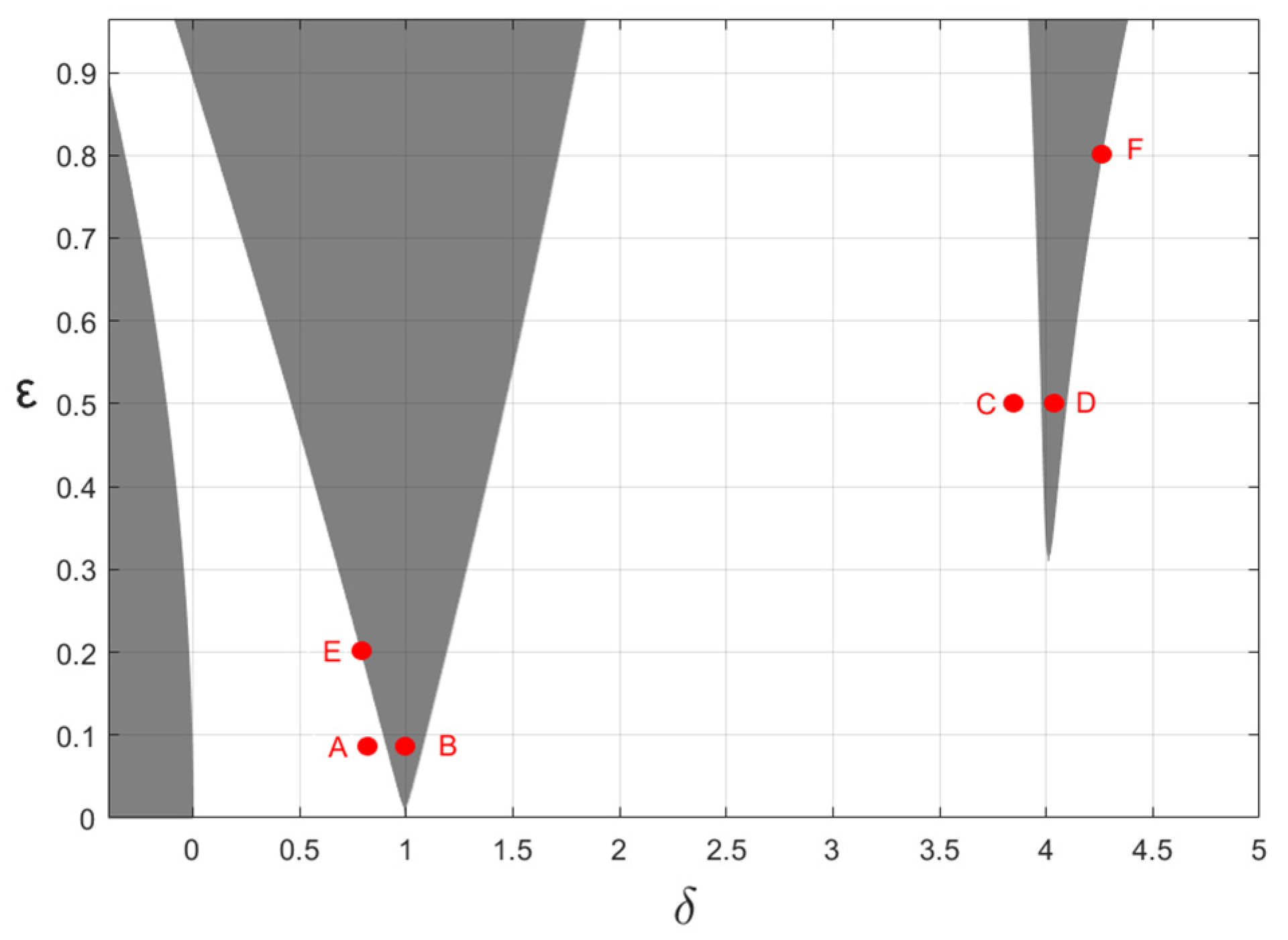
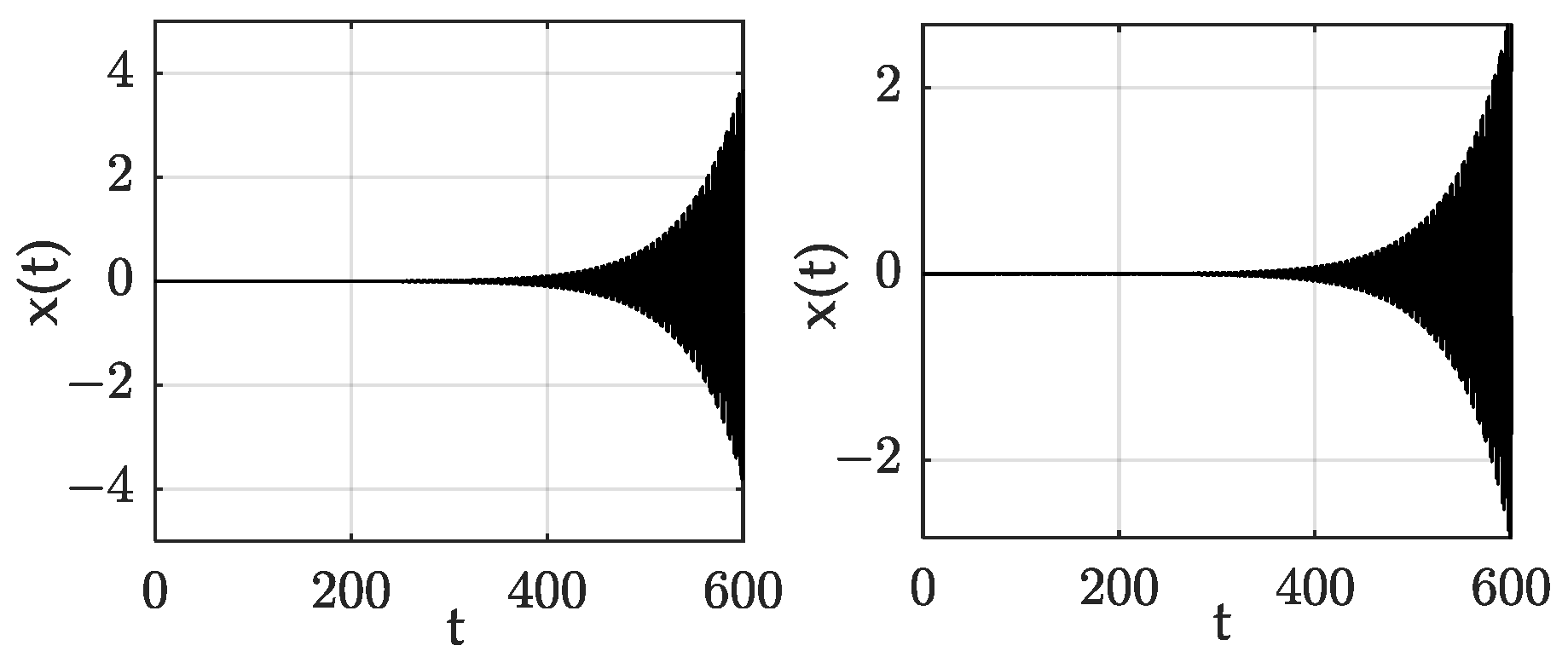
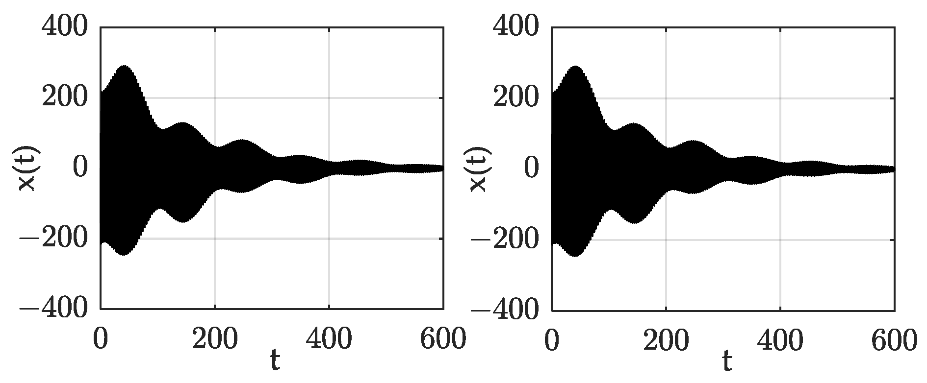
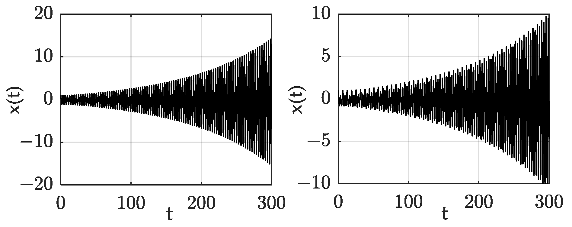
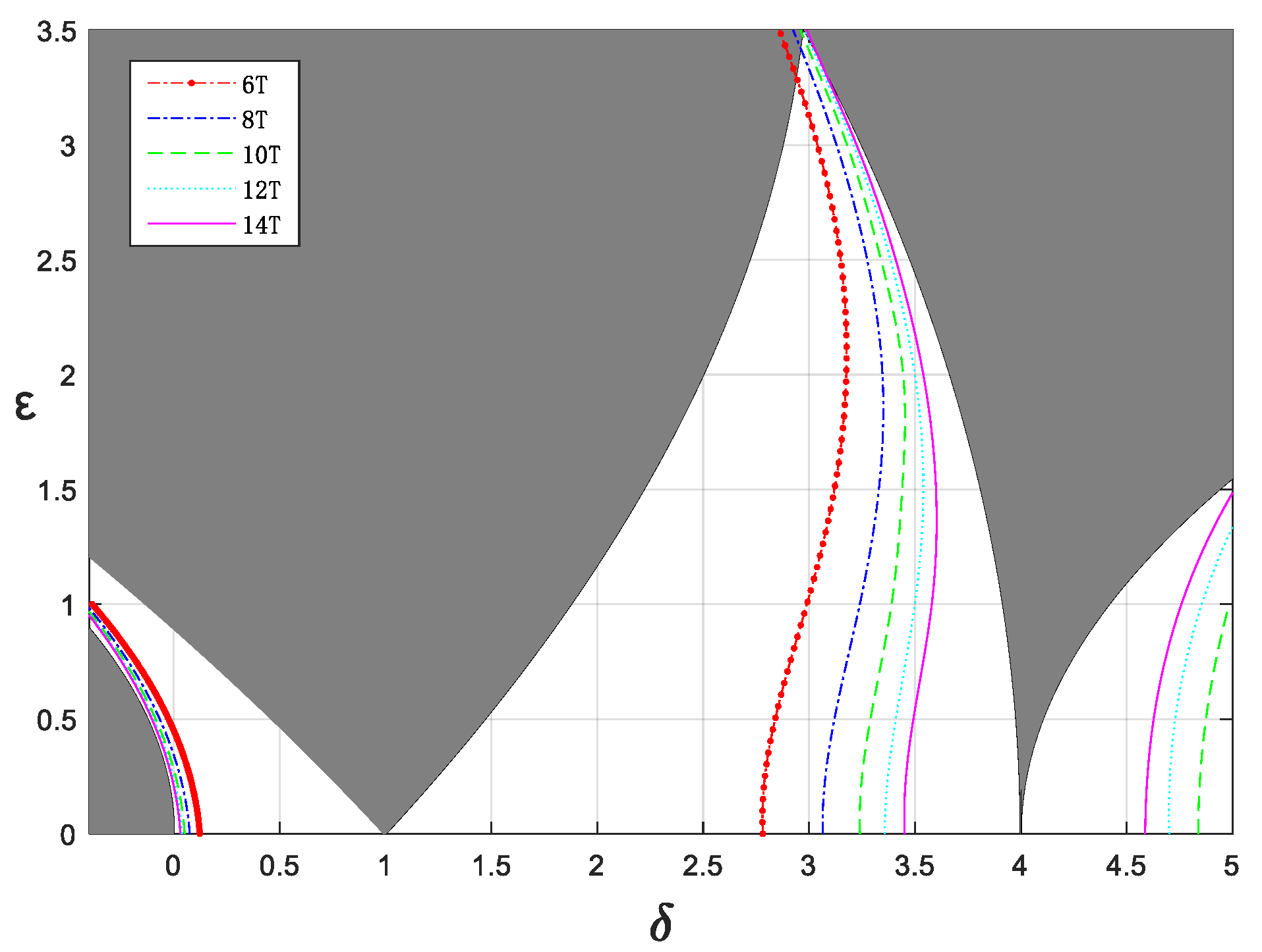
- Based on , when , the Floquet multipliers correspond to the -periodic solutions and -periodic solutions (corresponds to the stability boundary). For an inhomogeneous linear system, the forced excitation with finite period does not change the convergence of the stability boundary; only when the period of the forced excitation is large enough will the stability boundary become unstable.
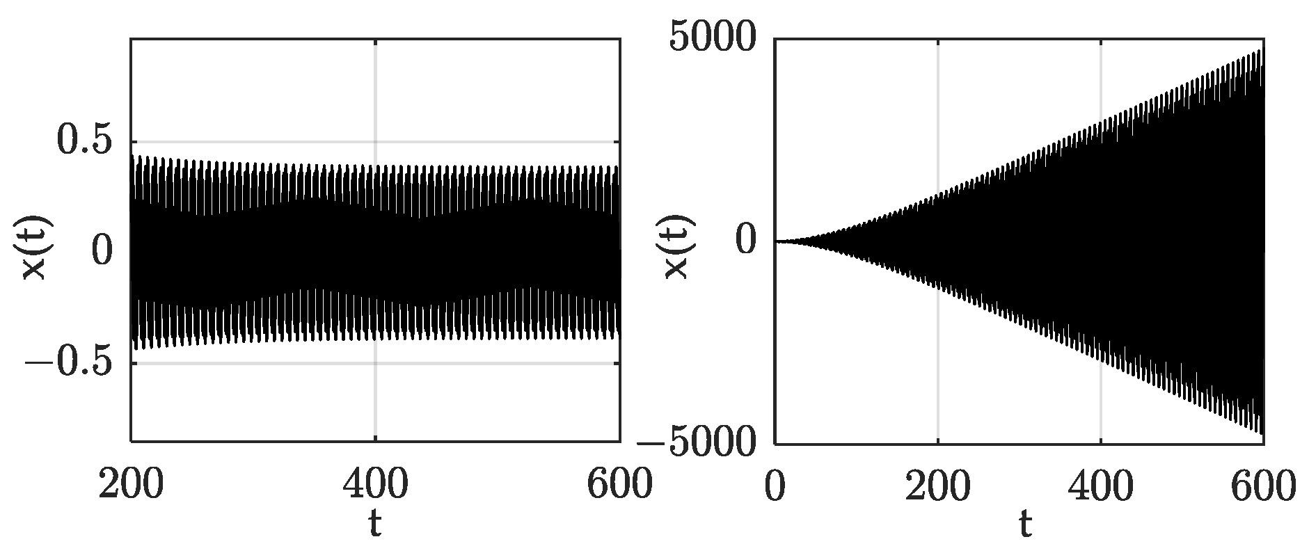
- 3.2
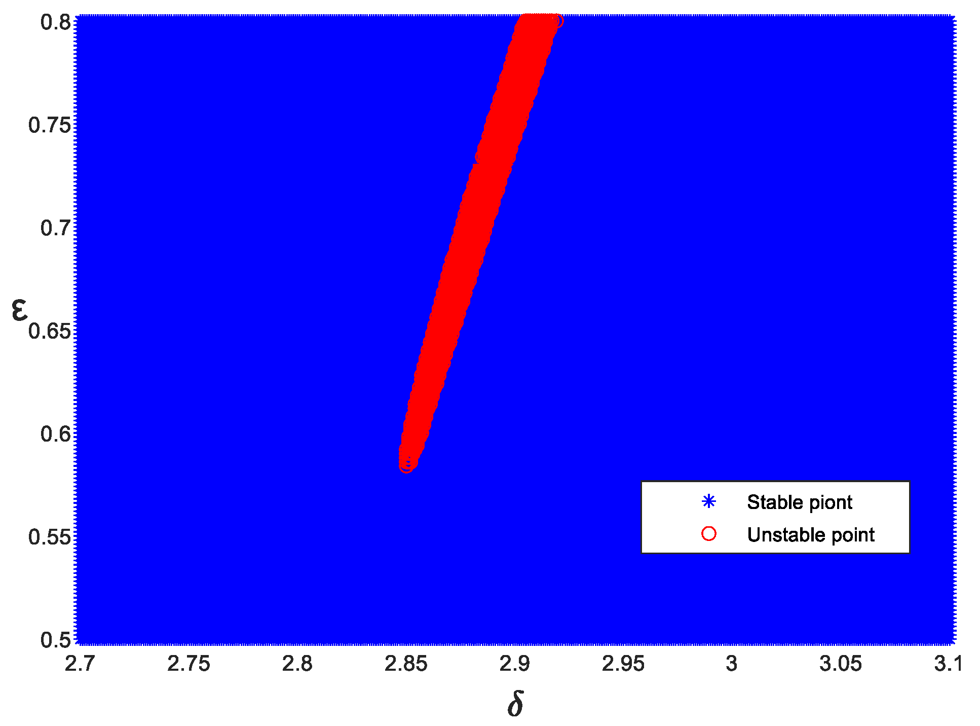
- When the Floquet multipliers are , they correspond to the periodic solutions in the system. Under the forced excitation with the same period, such k’T-periodic solution will become unstable due to resonance [28]. This will be described in more detail in Section 4.1.
- 3.3
- When there are multiple eigenvalues, not semisimple, the solutions of the system are unbounded in both homogeneous and inhomogeneous cases.
2.3. The Analytical Study of Stability Boundaries
- Let = 0
- 2.
- Choose
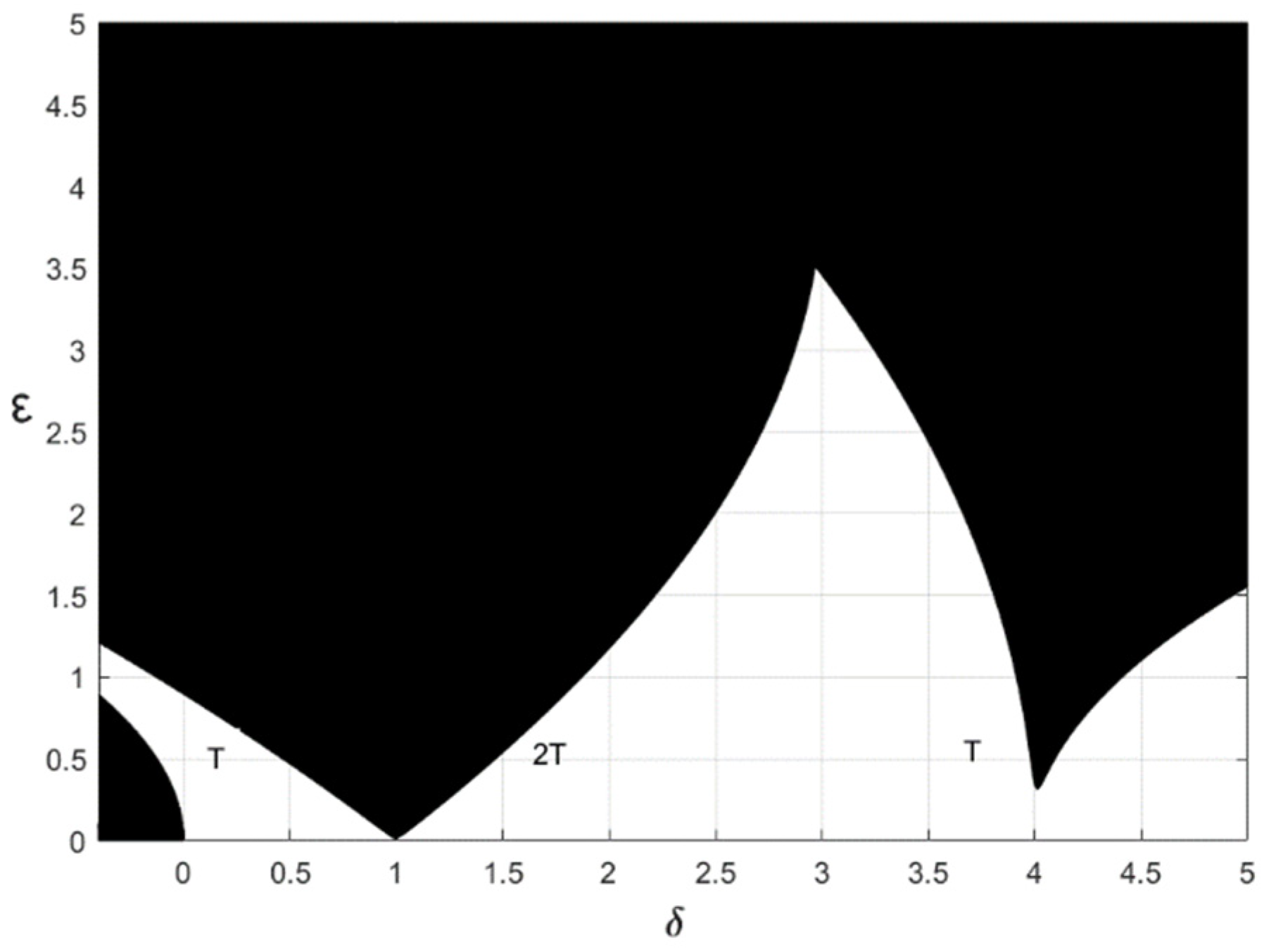
3. The Numerical Simulation of Stability Boundaries
3.1. Comparative Analysis of Numerical Results and Analytical Results
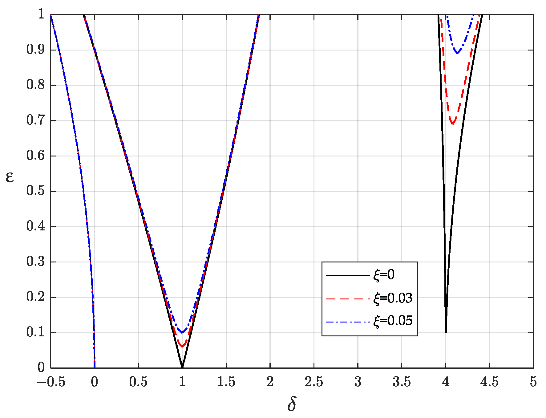
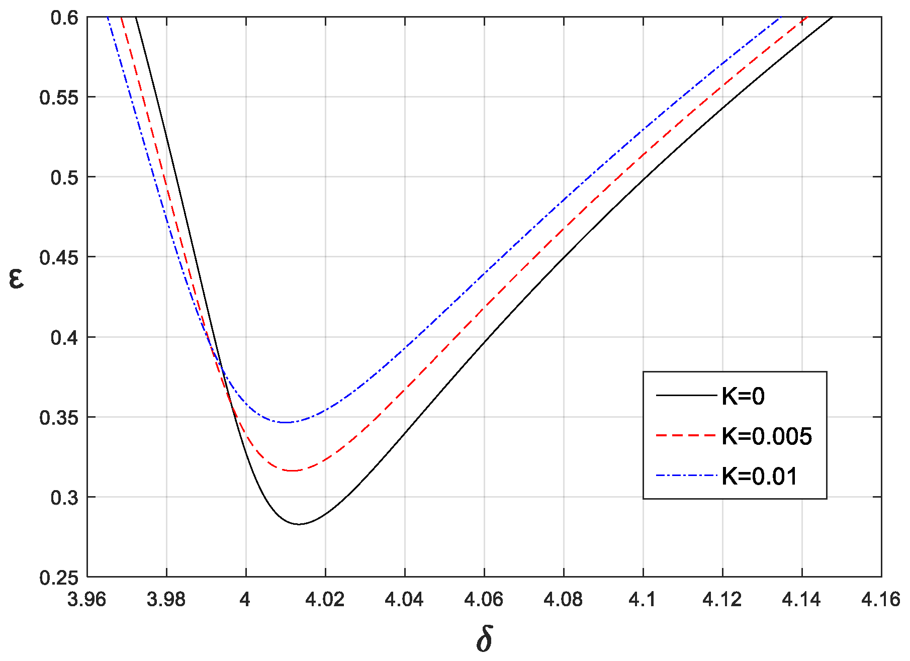
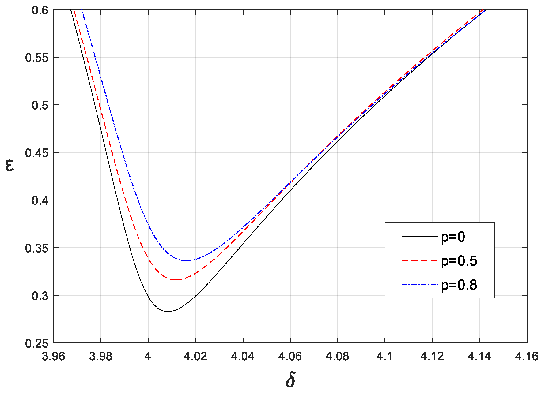
3.2. Effects of Damping and Fractional-Order Parameters on the Stability Boundaries
4. Stability Analysis of Periodic Solutions
4.1. Periodic Solutions in the Mathieu Equation
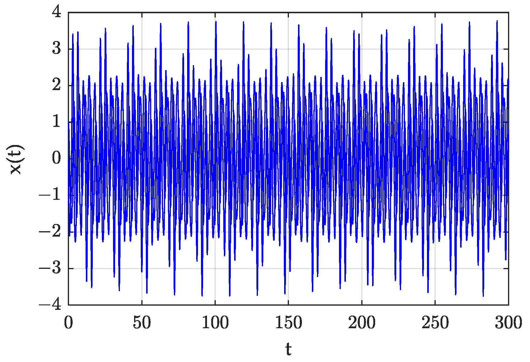
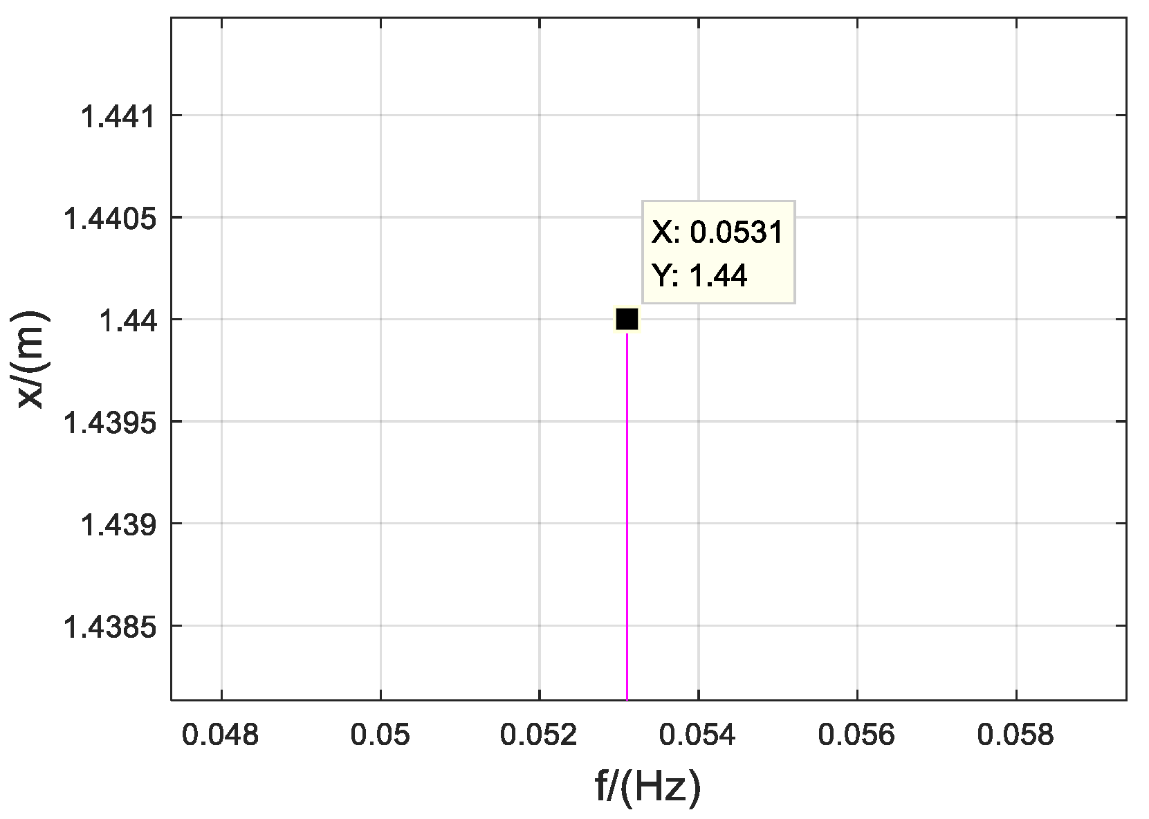
4.2. Numerical Simulation
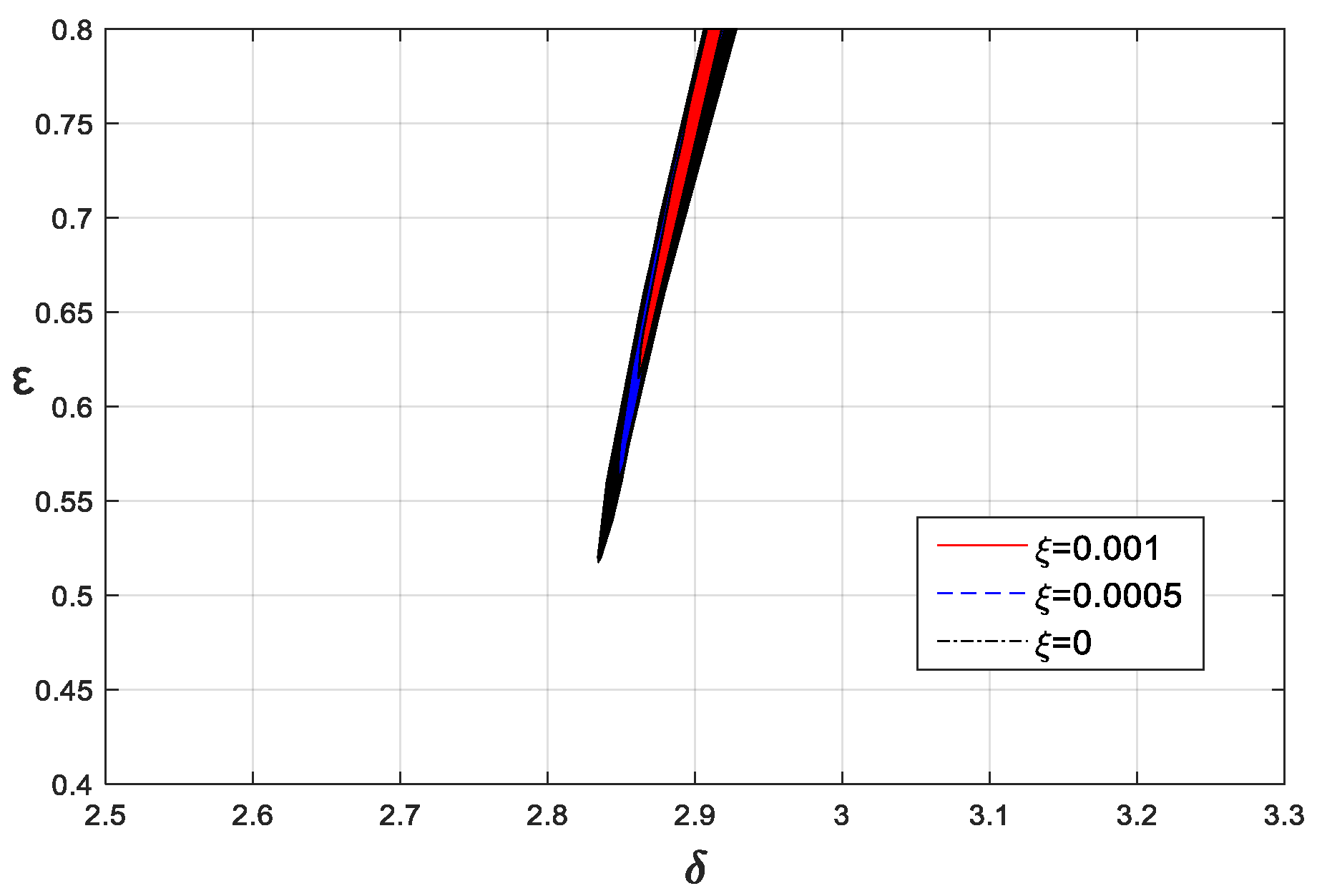
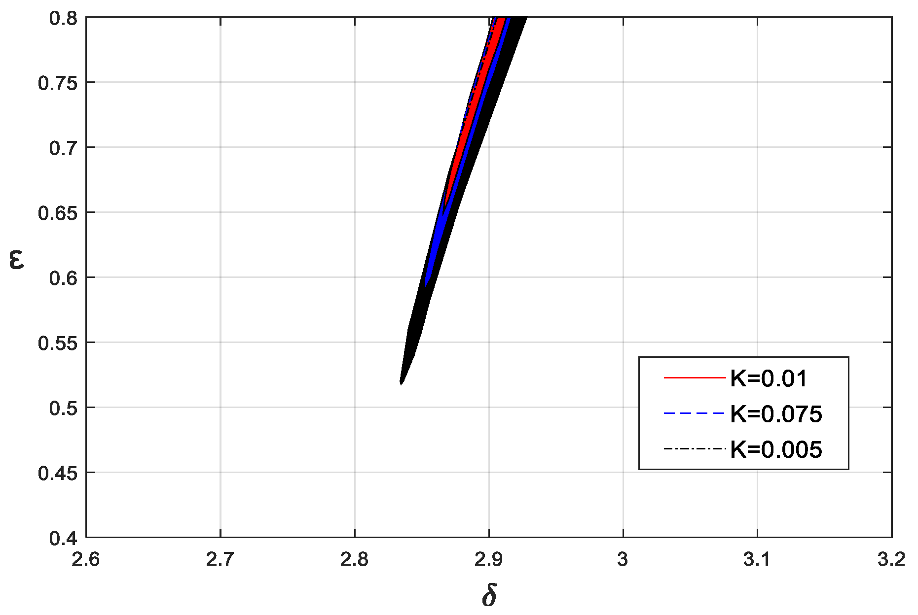
4.3. Effects of Damping and Fractional-Order Parameters on Resonance Lines
5. Conclusions
Author Contributions
Funding
Data Availability Statement
Conflicts of Interest
References
- Petras, I. Fractional-Order Nonlinear Systems: Modeling, Analysis and Simulation; Higher Education Press: Beijing, China, 2011; pp. 18–19. [Google Scholar]
- Podlubny, I. Fractional-Order Differential Equations; Academic Press: New York, NY, USA, 1999. [Google Scholar]
- Kilbas, A.; Srivastava, H.; Trujillo, J. Theory and Applications of Fractional-Order Differential Equations; Elsevier Science Limited: Amsterdam, The Netherlands, 2006. [Google Scholar]
- Ziada, E. Analytical Solution of Nonlinear System of Fractional Differential Equations. J. Appl. Math. Phys. 2021, 9, 2544–2557. [Google Scholar] [CrossRef]
- Mu’lla, M. Fractional Calculus, Fractional Differential Equations and Applications. Open Access Libr. J. 2020, 7, 1–9. [Google Scholar] [CrossRef]
- Wang, Q.; Xu, R. New Development on Fractional Order Calculus Operators. J. Binzhou Univ. 2021, 37, 51–58. [Google Scholar]
- Li, X.; Wang, Z. Modeling of Discrete Fracmemristor and Its Application in Logistic Mapping. Electron. Compon. Mater. 2022, 41, 627–634. [Google Scholar]
- Yang, J. Stabilization of Fractional Multiparameter Control Systems based on Cylindrical Algebraic Division Method. In Proceedings of the 33rd China Conference on Control and Decision-Making, Kunming, China, 22–24 May 2021; Volume 11, pp. 315–320. [Google Scholar] [CrossRef]
- Tang, J.; Li, X.; Wang, M. Dynamic Response and Vibration Isolation Effect of Generalized Fractional-Order Van Der Pol-Duffing Oscillator. Vib. Shock. 2022, 9, 10–18. [Google Scholar]
- He, X.; Hu, Z. Research on Optimal Design of Fractional Order Lowpass Filters. Acta Electron. Sin. 2022, 50, 185–194. [Google Scholar]
- Shen, Y.; Li, H.; Yang, S. Primary and Subharmonic Simultaneous Resonance of Duffing Oscillator. Nonlinear Dyn. 2020, 102, 1485–1497. [Google Scholar] [CrossRef]
- Qi, Z.; Wang, X.; Mo, R. Air Spring Modeling and Vehicle Dynamics Analysis Based on Fractional Calculus Theory. J. China Railw. Soc. 2021, 43, 67–76. [Google Scholar]
- Lu, Y.; Wang, C.; Deng, Q. The Dynamics of a Memristor-based Rulkov Neuron with Fractional-Order Difference. Chin. Phys. B 2022, 31, 46–54. [Google Scholar] [CrossRef]
- Chen, L.; Yin, H.; Huang, T. Chaos in Fractional-Order Discrete Neural Networks with Application to Image Encryption. Neural Netw. 2020, 125, 174–184. [Google Scholar] [CrossRef]
- Hou, J.; Yang, S.; Li, Q. Effects of Speed Feedback Fractional Order PID Control on Vibration Characteristics of Gear System. J. Vib. Shock. 2021, 40, 175–181. [Google Scholar]
- Chang, Y.; Tian, W.; Jin, G. Research on Nonlinear Fractional Active Control Suspension Based on Fractional Order PIλDμ. J. Yanshan Univ. 2020, 44, 575–580. [Google Scholar]
- Wang, L.; Cui, L.; Han, Z.; Ying, W. Parametric Excited Vibration Control of a SMA Beam under Fluctuating Temperature. J. Vib. Shock. 2022, 41, 135–138. [Google Scholar]
- Xu, M.; Li, L.; Ren, S. Numerical Method for Stability Analysis of Multiple-Degree-of-Freedom Parametric Dynamic Systems. Chin. J. Comput. Mech. 2020, 37, 48–52. [Google Scholar]
- Tang, Y.; Wang, L.; Liu, Z. Ship Nonlinear Dynamics Analysis Method and Its Engineering Applications. Ship Boat 2022, 33, 1–14. [Google Scholar]
- Zhu, D.; Xue, R.; Cao, X. Vehicle Random Vibration Analysis Using a SDOF Parametric Excitation Model. J. Vib. Shock. 2022, 41, 79–86. [Google Scholar]
- Li, G.; Zhu, Z.; Cheng, C. Dynamical Stability of Viscoelastic Column with Fractional Derivative Constitutive Relation. Appl. Math. Mech. 2001, 22, 294–303. [Google Scholar] [CrossRef]
- Wen, S. Dynamics and Control of Fractional-Order Parametrically Excited System. PhD. Dissertation, Shijiazhuang Tiedao University, Shijiazhuang, China, 2018; pp. 22–37. [Google Scholar]
- Guo, J.; Shen, Y.; Li, H. Dynamic Analysis of Quasi-periodic Mathieu Equation with Fractional-Order Derivative. Chin. J. Theor. Appl. Mech. Sin. 2021, 53, 3366–3375. [Google Scholar]
- Rodriguez, A.; Collado, J. Periodic Solutions in Non-Homogeneous Hill Equation. Nonlinear Dyn. Syst. Theory 2020, 20, 78–91. [Google Scholar]
- Yang, S.; Liu, Y. Development of Rail Vehicle Dynamics and Control. J. Dyn. Control. 2020, 18, 1–4. [Google Scholar]
- Tian, Q.; Zhang, B. Research on Application and Development Trend of Air Spring in Railway Vehicle. New Ind. 2021, 11, 173–174. [Google Scholar]
- Yakubovich, V.; Starzhinski, V. Linear Differential Equations with Periodic Coeffi-Cients; Wiley: New York, NY, USA, 1975. [Google Scholar]
- Slane, J.; Tragessser, S. Analysis of Periodic Nonautonomous Inhomogeneous Systems. Nonlinear Dyn. Syst. Theory 2011, 11, 183–198. [Google Scholar]
- Diethelm, K. The Analysis of Fractional-Order Differential Equations: An Application-Oriented Exposition Using Differential Operators of Caputo Type; Springer: New York, NY, USA, 2010. [Google Scholar]
- Abu-Shady, M.; Kaabar, M.K.A. A Generalized Definition of the Fractional Derivative with Applications. Math. Probl. Eng. 2021, 9, 9444803. [Google Scholar] [CrossRef]
- Abu-Shady, M.; Kaabar, M.K.A. A Novel Computational Tool for The Fractional-Order Special Functions Arising from Modeling Scientific Phenomena via Abu-Shady–Kaabar Fractional Derivative. Comput. Math. Methods Med. 2022, 5, 2138775. [Google Scholar] [CrossRef] [PubMed]


Publisher’s Note: MDPI stays neutral with regard to jurisdictional claims in published maps and institutional affiliations. |
© 2022 by the authors. Licensee MDPI, Basel, Switzerland. This article is an open access article distributed under the terms and conditions of the Creative Commons Attribution (CC BY) license (https://creativecommons.org/licenses/by/4.0/).
Share and Cite
Mu, R.; Wen, S.; Shen, Y.; Si, C. Stability Analysis of Fractional-Order Mathieu Equation with Forced Excitation. Fractal Fract. 2022, 6, 633. https://doi.org/10.3390/fractalfract6110633
Mu R, Wen S, Shen Y, Si C. Stability Analysis of Fractional-Order Mathieu Equation with Forced Excitation. Fractal and Fractional. 2022; 6(11):633. https://doi.org/10.3390/fractalfract6110633
Chicago/Turabian StyleMu, Ruihong, Shaofang Wen, Yongjun Shen, and Chundi Si. 2022. "Stability Analysis of Fractional-Order Mathieu Equation with Forced Excitation" Fractal and Fractional 6, no. 11: 633. https://doi.org/10.3390/fractalfract6110633
APA StyleMu, R., Wen, S., Shen, Y., & Si, C. (2022). Stability Analysis of Fractional-Order Mathieu Equation with Forced Excitation. Fractal and Fractional, 6(11), 633. https://doi.org/10.3390/fractalfract6110633