A Plea for the Integration of Fractional Differential Systems: The Initial Value Problem

Abstract

The usual approach to the integration of fractional order initial value problems is based on the Caputo derivative, whose initial conditions are used to formulate the classical integral equation. Thanks to an elementary counter example, we demonstrate that this technique leads to wrong free-response transients. The solution of this fundamental problem is to use the frequency-distributed model of the fractional integrator and its distributed initial conditions. Using this model, we solve the previous counter example and propose a methodology which is the generalization of the integer order approach. Finally, this technique is applied to the modeling of Fractional Differential Systems (FDS) and the formulation of their transients in the linear case. Two expressions are derived, one using the Mittag–Leffler function and a new one based on the definition of a distributed exponential function.

1. Introduction

The integration of Fractional Differential Equations (FDE) and Systems (FDS) is considered to be a well-founded and approved topic for most fractional calculus researchers. Therefore, the title of the paper appears as an ingenuous and unrealistic objective to revisit an established mathematical result. Nevertheless, our purpose is to provide an objective analysis of this fundamental problem and to formulate a satisfactory solution to fractional-order initial-value problems.

In fact, the initial-value problem, or Cauchy problem, is obviously trivial in the integer order case [1,2]. On the other hand, the solution of the fractional-order case appears as a generalization of the integer-order one. However, due to the multiplicity of fractional-order derivative definitions, researchers have considered it necessary to adapt the classical approach by referring to a particular derivative and its corresponding initial conditions [3,4,5]. Practically, most of the time, the Caputo derivative [3,6] is used because its “initial conditions” can be physically interpreted. Many critics have already addressed this choice, based on initialization considerations [7,8,9,10,11,12,13,14,15]. In those papers, the authors emphasize the inability of the Caputo derivative technique to solve the initialization problem, but, contrary to the history function technique [9,10,16,17,18,19,20,21] and the infinite-state approach [13,22,23,24], they do not provide a solution to this problem. Recently, some solutions based on new fractional derivatives (see, for example, [25,26,27,28]), which are in fact local derivatives [29,30], have been proposed. Practically, the direct consequence of these multiple choices is that different theoretical free responses are possible for the same FDE/FDS problem, which is of course physically inconsistent.

Our objective in this paper is to prove (in fact to recall) theoretically, using an elementary initial value problem, that the solution predicted by the Caputo derivative approach leads to a false free response. Then, we treat the same example with the frequency-distributed model of the fractional integrator [31,32,33,34]. We demonstrate that using a distributed initial condition, in fact that of the fractional integrator, provides the good solution to the considered problem. The conclusion of this analysis is that any fractional-order initial-value problem has to be treated such as in the integer-order case, using essentially the fractional integrator and its distributed initial state or its initialization function. Then, this technique is applied to the modeling of FDE/FDS and the formulation of their transients in the linear case. Two expressions are derived, one using the classic Mittag–Leffler function and a new one based on the definition of a distributed exponential function.

The theory developed in the paper is not a new one, since the first paper [35] related to the fractional integrator was published in 1999. Since that original publication, this research has been applied to the modeling and identification of real-world diffusive processes: electrochemical [36], thermal [37], and rotor skin effect, see chapter 5, volume 1 of [34]. The modeling of fractional systems based on the fractional integrator, known as the infinite-state approach, has been presented in several articles, see, for example, [22,33,38], with a particular focus on system initialization [23,24]. Moreover, it has been applied to the stability analysis of linear and nonlinear systems with a distributed formulation of the Lyapunov function [39]. The theory of the infinite state approach and its applications to various domains of control theory are presented in a two-volume monograph [34]. However, in spite of its contributions to initialization and Lyapunov system stability, this theory is ignored or considered as an exotic contribution to fractional calculus, although it has been adopted by researchers for initialization purposes [21,40,41,42] and Lyapunov stability analysis [43,44,45,46,47,48]. Moreover, although the pseudo initial conditions of the Caputo derivative are frequently criticized [8,9,16,20], mainly for their use in system initialization [7,14,15,21], they are still used because they provide apparently simple solutions. Consequently, there is an important challenge to provide a general and satisfactory solution to the initialization problem, using the same approach as in the integer-order case, where the initial conditions are those of the fractional integrator.

Thus, this paper intends to treat the FDE initial-value problem with a new and theoretical presentation of the infinite state approach, demonstrating that we do not have to refer to any fractional derivative and, on the contrary, can focus on the Riemann–Liouville integral and its distributed initial conditions. It is important to note that the authors have privileged a theoretical formalism contrary to their previous publications, where numerical simulations were abundantly used. So, the reader can refer to these previous papers to find numerical illustrations related to initialization. A restricted version of the paper has already been published in a recent conference [49].

The paper is composed of six sections and a conclusion. Section 1 is the introduction. Section 2, Section 3 and Section 4 present the materials and methods related to initial-value problems and the infinite state approach. In Section 5, an elementary counter-example permits us to invalidate the usual Caputo derivative initial value approach. In Section 6, the frequency-distributed integrator model is used to solve the previous counter-example and to formulate a new approach to the FDE initial-value problem. This methodology is used in Section 6 to express the dynamics of the general FDS initial-value problem.

2. Materials and Methods

2.1. The ODE Initial-Value Problem (or Cauchy Problem [1])

Let us consider the following Ordinary Differential System:

$$\frac{dx(t)}{dt}=f\left(x(t),u(t)\right)$$

(1)

where $x(t)=x(0) \mathrm{at} t=0$ is the initial value.

The Picard-Lindelöf theorem [50] guarantees the existence of a unique solution to (1). The principle of this theorem consists in reformulating the problem as an equivalent integral equation:

$$x(t)=I_t^1\left[\frac{dx(t)}{dt}\right]+x(0)={\displaystyle \underset{0}{\overset{t}{\int }}f\left(x(\tau ),u(\tau )\right)d\tau +x(0)}$$

(2)

and to construct a sequence of functions

$${\varphi }_{k+1}(t)={\displaystyle \underset{0}{\overset{t}{\int }}f\left({\varphi }_k(\tau ),u(\tau )\right)d\tau +x(0)} \mathrm{with} {\varphi }_1(t)=x(0),$$

(3)

which converges to the solution of (1) and thus to the solution of the initial-value problem.

Such a construction is called Picard’s method [51] or the method of successive approximations.

In the linear and multidimensional case, Equation (1) can be expressed as:

$$\frac{d\underset{¯}{x}(t)}{dt}=A\underset{¯}{x}(t)+Bu(t)\hspace{1em}x(t)=x(0)\hspace{1em}\mathrm{at}\mathrm{t}=0,$$

(4)

where x(t) ϵ R^N, and A and B are matrices of appropriate dimensions.

It is well known that its solution, based on the exponential matrix function or transition matrix

$$\Phi (t)=e^{At} \mathrm{with} \Phi \left(t\right)\in R^{N\times N}$$

is given by [52]:

$$x(t)=\Phi (t)x(0)+{\displaystyle \underset{0}{\overset{t}{\int }}\Phi (t-\tau )B}u(\tau )d\tau .$$

(5)

2.2. The FDE/FDS Initial Value Problem

Let us consider the elementary FDE

$$D_t^n\left(x(t)\right)=f\left(x(t),u(t)\right)\hspace{1em}0<n<1,$$

(6)

where n is the fractional order and x(t) = x(0) at t = 0.

Contrary to the integer-order case, several approaches are derived from the fractional derivative definitions of $D_t^n\left(x(t)\right).$ The main popular ones are the Caputo and Riemann–Liouville derivatives [3].

Practically, Equation (6) is integrated with the Caputo derivative definition, since its initial condition is considered equal to x(0).

Then, in order to prove the existence and the uniqueness of the solution x(t) of (6), Picard’s method [3,4,5] is frequently used.

In the linear multidimensional commensurate order case, Equation (6) becomes:

$$\left\{\begin{array}{cc}\begin{array}{c}{D}_t^n\left(\underset{¯}{x}(t)\right)=A\underset{¯}{x}(t)+Bu(t)\\ y(t)=\underset{¯}{C}x(t)\end{array}& 0<n<1,\end{array}\right.$$

(7)

where x(t) ϵ R^N, and A and B are matrices of appropriate dimensions.

The general solution of (7), expressed in terms of the Mittag–Leffler matrix function [53]

$$\Phi (t)=E_{n,1}\left(A{t}^n\right), \Phi \left(t\right)\in R^{N\times N}$$

is

$$\underset{¯}{x}(t)=\Phi (t)\underset{¯}{x}(0)+{\displaystyle \underset{0}{\overset{t}{\int }}\Phi (t-\tau )B}\tilde{u}(\tau )d\tau \hspace{1em}\mathrm{with} \tilde{u}(\tau )=D^{1-n}\left(u(\tau )\right).$$

(8)

As mentioned in the introduction, the main objective of this paper is to revisit the integration of the FDE/FDS initial-value problem, using the infinite-state approach, which is directly related to the integer order ODE case and does not need any derivative definition, as it is exhibited in Section 4.

3. Integration of FDE/FDS Based on Derivative Definitions

3.1. Riemann–Liouville Integral

The fractional integral of a function v(t), also called the Riemann–Liouville integral is defined by

$$x(t)={}_{0}I_t^n\left(f(t)\right)={\displaystyle \underset{0}{\overset{t}{\int }}\frac{{(t-\tau )}^{n-1}}{\Gamma (n)}}v(\tau )d\tau \hspace{1em}0<n<1,$$

(9)

where (n) is the gamma function.

The fractional integral is in fact a convolution integral, characterized by the impulse response or Kernel, $h_n(t)$, such that:

$$h_n(t)=\frac{t^{n-1}}{\Gamma (n)} and x(t)=h_n(t)\ast v(t).$$

(10)

Using the Laplace transform, we obtain

$$L\left\{h_n(t)\right\}=\frac{1}{s^n},$$

(11)

where $\frac{1}{s^n}$ corresponds to the fractional order integration operator.

3.2. Fractional Derivatives Definitions

Contrary to the fractional integral, the fractional derivative is not uniquely defined. Usually, two main derivatives are considered; since they are used for the integration of FDE/FDS, we focus on the case 0 < n < 1 [34].

3.2.1. Caputo Derivative Definition

This definition corresponds to first differentiate x(t) and then calculates a fractional integral with order (1−n). Since 0 < n < 1, then 0 < 1−n < 1.

$${}^{C}D_t^n\left(x(t)\right)=I_t^{1-n}\left(\frac{dx}{dt}\right)=h_{1-n}(t)\ast \frac{dx}{dt}$$

(12)

Definition (12) clearly shows that the Caputo derivative corresponds to the Riemann–Liouville integral of the derivative of x(t).

In the Laplace domain, the Caputo derivative definition leads to

$$L\left\{\left({}^{C}D_t^n(x)\right)\right\}=\frac{1}{s^{1-n}}L\left\{\frac{dx(t)}{dt}\right\}=\frac{1}{s^{1-n}}\left[sX(s)-x(0)\right].$$

(13)

$$\mathrm{So}, X(s)=\frac{1}{s^n}L\left\{{}^{C}D_t^n(x)\right\}+\frac{x(0)}{s},$$

(14)

Or in the time domain,

$$x(t)=I_t^n\left({}^{C}D_t^n(x)\right)+x(0).$$

(15)

Thus, the solution of FDE/FDS (6) according to the Caputo approach is

$$\begin{array}{ccc}x(t)={}_{0}I_t^n\left(f\left(x(t),u(t)\right)\right)+x(0)& \mathrm{for} \mathrm{t}\ge 0& 0<n<1,\end{array}$$

(16)

where $x\left(0\right)$ is interpreted as the initial condition of the FDE/FDS and also as the initial value of the Riemann–Liouville integral.

This simple integral Equation (16), apparently equivalent to the integer order case (2), has made the success of the Caputo derivative approach.

3.2.2. Riemann–Liouville Derivative Definition

This definition shows that the Riemann–Liouville derivative corresponds to the integer-order derivative of the Riemann–Liouville integral of x(t).

$${}^{RL}D_t^n\left(x(t)\right)=\frac{d}{dt}\left[I_t^{1-n}(x)\right]=\frac{d}{dt}\left[h_{1-n}(t)\ast x(t)\right]$$

(17)

Using the Laplace transform, we obtain

$$\begin{array}{l}L\left\{{}^{RL}D_t^n(x)\right\}=s\left(L\left\{I_t^{1-n}(x)\right\}\right)-g(0)=s\left(\frac{1}{s^{1-n}}X(s)\right)-g(0)=s^{n}X(s)-g(0)\\ \mathrm{with} \mathrm{g}\left(0\right)={\left\{{}_{-\infty }I_t^{1-n}(x)\right\}}_{t=0}\end{array}.$$

Since g(0) does not have a physical and direct interpretation, the Riemann–Liouville derivative is generally not used to integrate system (6) or (7).

It is important to note that the two derivative definitions only require integer-order differentiation $\left(\frac{d}{dt}\right)$ and fractional-order integration $\left(I^{1-n}\right)$. So, contrary to a common belief, the basic operation of fractional calculus is not fractional differentiation but fractional integration.

3.2.3. The Grünwald–Letnikov Derivative

Instead of the two previous fractional derivatives, it is possible to use the Grünwald-Letnikov (G.L.) derivative, with appropriate initial conditions. In fact, it is preferable to consider the G.L. integrator that corresponds to the discretization of the Riemann–Liouville integral.

The Nth integer order Euler derivative of x(t) is defined as

$${\left(D^N\left(x(t)\right)\right)}_{t=k{T}_e}=\underset{T_e\to 0}{\lim }\frac{{\left(1-q^{-1}\right)}^N}{{T_e}^N}{x}_k,$$

(18)

where T_e is the sample time, $x_k=x(k{T}_e)$, and $q^{-1}$ is the delay operator.

The generalization to the fractional order case provides the Grünwald–Letnikov derivative

$${\left({}^{GL}D^n\left(x(t)\right)\right)}_{t=k{T}_e}=\underset{T_e\to 0}{\lim }\frac{{\left(1-q^{-1}\right)}^n}{{T_e}^n}{x}_k 0<n<1.$$

(19)

Since $L\left\{q^{-1}\right\}=e^{-T_{e}s}$, we obtain

$$L\left\{{}^{GL}D^n\left(x(t)\right)\right\}=\underset{T_e\to 0}{\lim }\frac{{\left(1-e^{-T_{e}s}\right)}^n}{{T_e}^n}L\left\{x(t)\right\}=s^{n}X(s).$$

(20)

Notice that

$$\frac{{\left(1-q^{-1}\right)}^n}{{T_e}^n}=\frac{1}{{T_e}^n}\left[1+{\displaystyle \sum _{i=0}^{\infty }{\alpha }_{i,GL}{q}^{-i}}\right],$$

(21)

with ${\alpha }_{i,GL}={(-1)}^i\frac{n}{1}\frac{n-1}{2}\frac{n-2}{3}\dots \dots \frac{n-(i+1)}{i}$,

$$\mathrm{so} {\left({}^{GL}D^n\left(x(t)\right)\right)}_{t=k{T}_e}=\frac{1+{\displaystyle \sum _{i=0}^{\infty }{\alpha }_{i,GL}{q}^{-i}}}{{T_e}^n}{x}_k,$$

(22)

which is the Moving Average formulation of the Grünwald–Letnikov derivative.

Reciprocally, we can define the Grünwald–Letnikov integral operator [34] as

$${}^{GL}I^n\left(f_k\right)=\frac{{T_e}^n{q}^{-1}}{1+{\displaystyle \sum _{i=0}^{\infty }{\alpha }_{i,GL}{q}^{-i}}}{f}_k,$$

(23)

which is the Auto-Regressive formulation of the Grünwald–Letnikov integrator.

Notice that

$$L\left\{{}^{GL}I^n\left(f(t)\right)\right\}=\underset{T_e\to 0}{\lim }\frac{{T_e}^n{e}^{-T_{e}s}}{{\left(1-e^{-T_{e}s}\right)}^n}L\left\{f(t)\right\}=\frac{1}{s^n}F(s),$$

(24)

which means that the Grünwald–Letnikov integrator is the time discretization of the Riemann–Liouville integral.

Consider now the elementary FDE initial value problem (6):

$$\begin{array}{cc}{D}_t^n\left(x(t)\right)=f\left(x(t),u(t)\right)& 0<n<1.\end{array}$$

Using the Grünwald–Letnikov integrator, we can express $\left\{x(k)\right\}$ as:

$$\left\{x(k+1)\right\}={}^{GL}I^n\left(f\left(\left\{xk\right\},\left\{uk\right\}\right)\right)+g\left\{x_{init}\right\},$$

(25)

where $\left\{x_{init}\right\}=\left\{x(0),x(-1),\dots \dots ,x(-i),\dots \dots ,x(-\infty )\right\}$.

This means that the initial conditions are composed of all the past values of $x(-i)$, since $k=-\infty$.

Practically, this technique is used for the numerical simulation of the FDE/FDS problem.

The interested reader can refer to chapter 3 volume 1 of [34], where different initializations of the G.L. integral and the short memory principle [3] are analyzed.

4. The Infinite State Approach

4.1. Introduction

The infinite-state approach (do not confuse it with diffusive representation, see chapter 7 of [34]) is a modeling technique based on the fractional-integration operator, which is at the heart of any modeling and simulation system, either integer or fractional order, linear or non-linear [22,52].

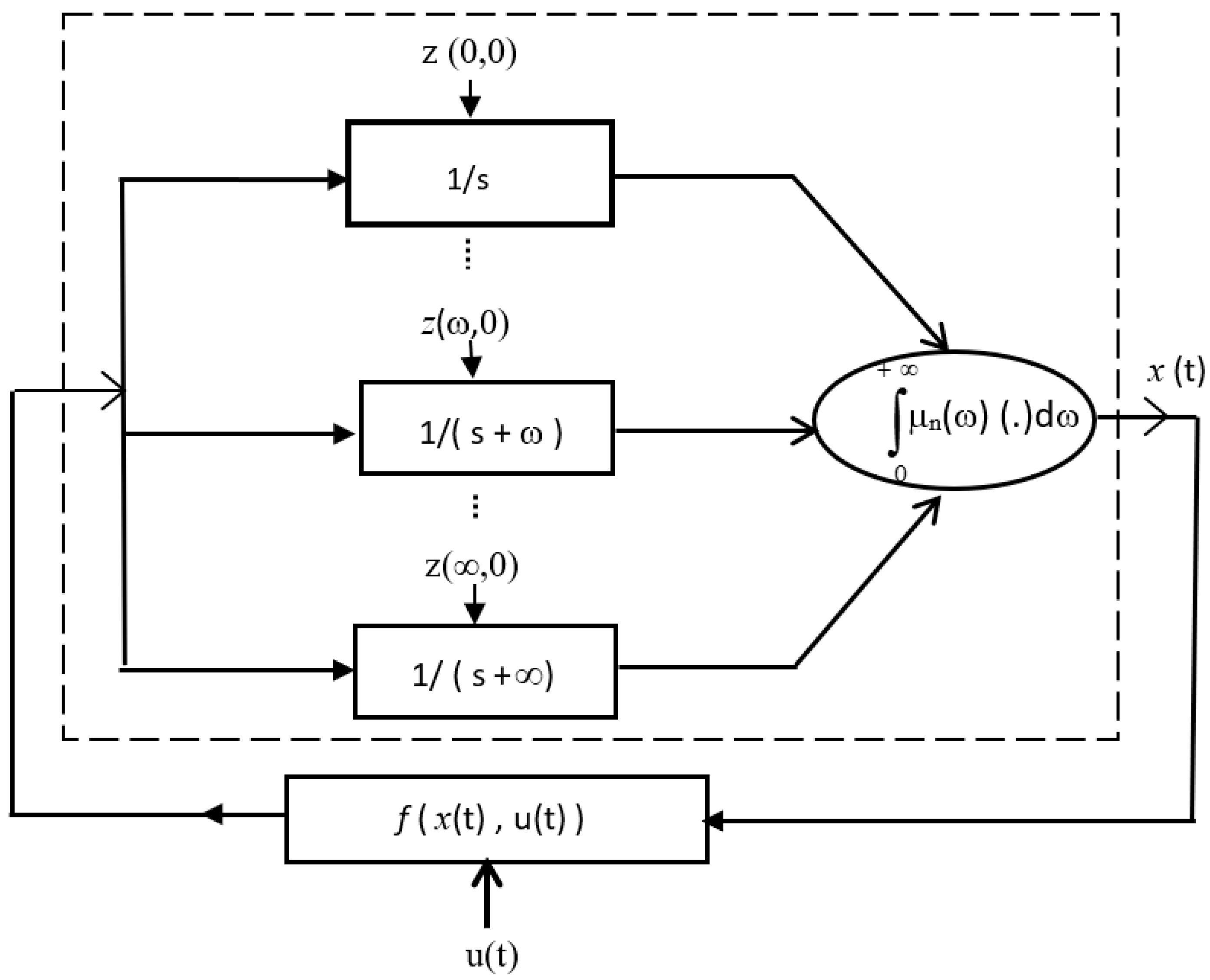
4.2. The Frequency-Distributed Model of the Fractional Integrator

As shown in Section 3, the Riemann–Liouville integral of a function $v(t)$ is defined as the convolution of $v(t)$ with the impulse response $h_n(t)$ of the fractional integrator.

Another expression of $h_n(t)$ can be derived from the inverse Laplace transform of $\frac{1}{s^n}$ [31,32,34], for 0 < n < 1, i.e., $h_n(t)=L^{-1}\left\{\frac{1}{s^n}\right\}$.

Using a Bromwich contour, we can write (see [34] and the references therein):

$$h_n(t)=\left\{\begin{array}{ll}\frac{1}{2\pi j}{\displaystyle \underset{\gamma -j\omega }{\overset{\gamma +j\omega }{\int }}\frac{1}{s^n}{e}^{st} ds}& \mathrm{for} \mathrm{t}>0\\ 0& \mathrm{for} \mathrm{t}<0\end{array}\right..$$

Thus, we obtain

$$\begin{array}{ll}{h}_n(t)={\displaystyle \underset{0}{\overset{\infty }{\int }}{\mu }_n(\omega )e^{-\omega t}}d\omega =\frac{t^{n-1}}{\Gamma (n)}& \mathrm{for} 0<n<1\\ \mathrm{with} {\mu }_n(\omega )=\frac{\sin (n\pi )}{\pi }{\omega }^{-n}& \end{array}$$

(26)

Note that, in the particular case where v(t) = (t) is an impulse function, the output x(t) corresponds to the impulse response $h_n(t)$ and is provided by the following distributed integer-order differential system

$$\left\{\begin{array}{c}\frac{\partial z(\omega ,t)}{\partial t}=-\omega z(\omega ,t)+\delta (t)\hspace{1em}\omega \in \left[0,+\infty \right)\\ h_n(t)={\displaystyle \underset{0}{\overset{\infty }{\int }}\mu (\omega )z(\omega ,t)d\omega }\end{array}\right.$$

(27)

Thus $z(\omega ,t)=e^{-\omega t}$, which leads to $h_n(t)={\displaystyle \underset{0}{\overset{\infty }{\int }}\mu (\omega )e^{-\omega t}d\omega }$.

More generally, for any input v(t), the corresponding output x(t) of the fractional integrator is provided by the following distributed frequency system:

$$\left\{\begin{array}{c}\frac{\partial z(\omega ,t)}{\partial t}=-\omega z(\omega ,t)+v(t)\hspace{1em}\omega \in \left[0,\infty \right)\\ x(t)={\displaystyle \underset{0}{\overset{\infty }{\int }}{\mu }_n(\omega )z(\omega ,t)d\omega }\\ \mathrm{with} {\mu }_n(\omega )=\frac{\sin (n\pi )}{\pi }{\omega }^{-n}\end{array}\right.$$

(28)

It is fundamental to notice that the original model of the fractional integrator has been transformed into an infinite-dimension integer-order differential system (28), where integer-order differentiation $\frac{\partial }{\partial t}$ has been substituted to fractional-order differentiation, and where the fractional order $n$ appears in the weighting function ${\mathsf{\mu }}_n(\omega )$. This means that the fractional integrator $\frac{1}{s^n}$ is an infinite-dimension linear system [54]. These models are the two “faces” of the fractional integrator.

In fact, according to linear system theory [52], the fractional integrator has two types of models, as does any other linear system:

-

the Equation $\mathrm{X}(s)=\frac{1}{s^n}V(s)$ is the input/output representation of the fractional integrator, characterized by its impulse response $h_n(t)$ and its frequency response $\frac{1}{{\left(j\omega \right)}^n}$.

-

the distributed differential system (28) is the infinite-dimension state-space model of the integrator, where the internal state $z(\omega ,t)$ permits a complete representation of system dynamics and particularly its free response from an initial condition $z(\omega ,0)$.

Remark 1:

let us consider the Laplace transform of (27):

$$L\left\{h_n(t)\right\}=L\left\{{\displaystyle \underset{0}{\overset{\infty }{\int }}\mu (\omega )e^{-\omega t}d\omega }\right\}={\displaystyle \underset{0}{\overset{\infty }{\int }}{\mu }_n(\omega )L\left\{e^{-\omega t}\right\}}d\omega ={\displaystyle \underset{0}{\overset{\infty }{\int }}{\mu }_n(\omega )\frac{1}{s+\omega }}d\omega$$

The previous equality and Equation (11) lead to

$$\begin{array}{cc}\frac{1}{s^n}={\displaystyle \underset{0}{\overset{\infty }{\int }}{\mathsf{\mu }}_n(\omega )\frac{1}{s+\omega }}d\omega & 0<n<1.\end{array}$$

(29)

This relation exhibits that the fractional integrator is composed of an infinity of modes $\omega ,$ ranging from 0 to $+\infty$, whereas the integer-order integrator corresponds to only one mode situated at $\omega =0$. Figure 1 displays the graphic representation of Equation (28). Note that the distributed differential Equations of (28) correspond to the first-order systems displayed in Figure 1. Due to the distributed nature of the differential system, the graph of Figure 1 is composed of an infinity of first-order systems.

Remark 2:

The classical Laplace transform of the integer order derivative is known as $L\left\{\frac{dx(t)}{dt}\right\}=sX(s)-x(0)$, which corresponds in fact to the relation $\mathrm{X}(s)=\frac{1}{s}L\left\{\frac{dx(t)}{dt}\right\}+\frac{x(0)}{s}$ i.e., in the time domain, to $x(t)={\displaystyle \underset{0}{\overset{t}{\int }}\frac{dx(\tau )}{d\tau }}d\tau +x(0)$, which means that $x(0)$ is not the initial condition of the derivative but is, in fact, the initial condition of the integrator which has memorizing capability.

4.3. Transients of the Fractional Integrator

Consider the Laplace transform of (28):

$$\left\{\begin{array}{c}sZ(\omega ,s)-z(\omega ,0)=-\omega Z(\omega ,s)+V(s)\hspace{1em}\omega \in \left[0,\infty \right)\\ X(s)={\displaystyle \underset{0}{\overset{\infty }{\int }}{\mu }_n(\omega )Z(\omega ,s)d\omega }\end{array}\right.$$

(30)

where $z(\omega ,0)$ is the initial value of $z(\omega ,t)$ at $t=0$.

This means that $Z(\omega ,s)=\frac{z(\omega ,0)}{s+\omega }+\frac{\mathrm{V}(s)}{s+\omega }$

$$\mathrm{and} X(s)={\displaystyle \underset{0}{\overset{\infty }{\int }}{\mu }_n(\omega )\frac{z(\omega ,0)}{s+\omega }}d\omega +{\displaystyle \underset{0}{\overset{\infty }{\int }}{\mu }_n(\omega )\frac{\mathrm{V}(s)}{s+\omega }}d\omega$$

(31)

Since $\frac{1}{s^n}={\displaystyle \underset{0}{\overset{\infty }{\int }}{\mu }_n(\mathsf{\omega })\frac{1}{s+\mathsf{\omega }}}d\mathsf{\omega }\hspace{1em}0<n<1$

we can write in the time domain:

$$x(t)={\displaystyle \underset{0}{\overset{\infty }{\int }}{\mu }_n(\omega )z(\omega ,0)e^{-\omega t}}d\omega +{}_{0}I_t^n\left(v(t)\right)$$

(32)

where:

-

$x(t)={\displaystyle \underset{0}{\overset{\infty }{\int }}{\mathsf{\mu }}_n(\mathsf{\omega })z(\mathsf{\omega },0)e^{-\omega t}}d\mathsf{\omega }$ is the free response of the fractional integrator initialized by the distributed initial conditions $z(\mathsf{\omega },0)\hspace{1em}\forall \mathsf{\omega }\in \left[0,\infty \right)$.

-

$I_t^n\left(v(t)\right)$ is the forced response of the fractional integrator caused by the input $v(t)$.

Previously, using the definition of the Caputo derivative “initial condition”, we wrote (20) $x(t)=I_t^n\left(v(t)\right)+x(0)$.

The conclusion is that this expression of the free response is wrong, since ${\displaystyle \underset{0}{\overset{\infty }{\int }}{\mathsf{\mu }}_n(\mathsf{\omega })z(\mathsf{\omega },0)e^{-\omega t}}d\mathsf{\omega }$ is the initialization function of the integrator. In fact, $x(0)={\displaystyle \underset{0}{\overset{\infty }{\int }}{\mathsf{\mu }}_n(\mathsf{\omega })z(\mathsf{\omega },0)}d\mathsf{\omega }$, and Equation (15) is correct only at $t=0$ and is wrong for t > 0.

The conclusion is that the fractional-integrator transients require to refer to its distributed model.

Basically, the initial condition of the differential system $D_t^n\left(x(t)\right)=f\left(x(t),u(t)\right)$ is related to the initial condition of the fractional integrator $\frac{1}{s^n}$ used for the integration of the FDE/FDS, not to the pseudo-initial condition of any fractional derivative. Notice that if this FDE/FDS is related to a real system, its dynamics must not depend on the fractional derivative definition choice of the user.

5. A Counter Example

In previous papers related to the infinite-state representation, we have already demonstrated that the so-called initial conditions of the Caputo derivative are unable to correctly express the dynamics of FDE/FDS free responses. However, attracted by the apparent simplicity of the Caputo initial conditions, most fractional calculus researchers ignore the more complex (in fact not too complex) infinite-state approach.

Consequently, this paper intends to prove the fundamental errors of the usual Caputo derivative approach using an elementary theoretical counter example. Then, with the frequency-distributed integrator allowing the theoretical computation of the true free response, we prove the necessity to use frequency-distributed initial conditions to solve any FDE/FDS initial-condition problem.

5.1. Problem Formulation

Consider the simplest FDE initial value problem

$$\left\{\begin{array}{c}{D}^n\left(x(t)\right)=u(t)\hspace{1em}0<n<1\\ x(t)=x(0) at t=0\end{array}\right.$$

(33)

Consider the special function $u(t)$, composed of two delayed Heaviside functions, $UH\left(t\right)$ and $-UH\left(t-T\right)$, with $u\left(t\right)=UH\left(t\right)-UH\left(t-T\right)$.

Consequently, see Figure 2

$$u(t)=\left\{\begin{array}{cc}U\hfill & for 0\le t<T\\ 0& for t\ge T\end{array}\right.$$

(34)

Moreover, assume that the system is at rest at $t=0$, i.e., $x\left(0\right)=0$.

Remark 3:

The interest of this example is to create a realistic initial condition at t = T, where the free response can be calculated with two approaches, the first one from t = 0 with no ambiguity using usual fractional calculus theory and the second one from t = T, using Equation (15) at $t_0=T$.

5.2. The Exact Solution

Since $x\left(0\right)=0$, we obtain $x(t)=I_t^n\left(UH(t)-UH(t-T)\right)=x^{+}(t)+x^{-}(t)$.

So $x^{+}(t)=h_n(t)\ast UH(t)={\displaystyle \underset{0}{\overset{t}{\int }}\frac{{(t-\mathsf{\tau })}^{n-1}}{\Gamma (n)}UH(\mathsf{\tau })d\mathsf{\tau }}=\frac{t^n}{\Gamma (n+1)}UH(t)$ and $x^{-}(t)=-h_n(t)\ast UH(t-T)=-\frac{{(t-T)}^n}{\Gamma (n+1)}UH(t-T)$.

Consequently, see Figure 2 (for n = 0.5):

$$x(t)=\left\{\begin{array}{c}\frac{t^{n}U}{\Gamma (n+1)}\hspace{1em}for 0\le t\le T\\ \frac{U}{\Gamma (n+1)}\left[t^n-{(t-T)}^n\right]\hspace{1em}for t\ge T\end{array}\right.$$

(35)

where $x(t) for t\ge T$ represents the free response of (33) at $t_0=T$.

5.3. Solution Derived from the Caputo Derivative Definition

This free response can also be expressed using Equation (15) at $t_0=T$ with $x\left(t_0\right)=x\left(T\right)$, i.e., $x(t)=I_t^n\left(u(t)\right)+x(T) for t\ge T$.

Thus (see Figure 2),

$$x(t)=x(T)\hspace{1em}for t\ge T$$

(36)

This result is obviously in complete contradiction with Equation (35), i.e., $x(t)=\frac{U}{\Gamma (n+1)}\left[t^n-{(t-T)}^n\right] for t\ge T$.

Notice that, for $n=1$, we obtain:

$x(T)=UT\hspace{1em}for t=T$ and $x(t)=U\left[t-(t-T)\right]=UT\hspace{1em}for t\ge T$.

Thus, we verify that $x(t)=x(T)\hspace{1em}for t\ge T$, i.e., Equation (36) is only correct in the integer-order case.

With this very simple example, we have demonstrated that Equation (15) is wrong in the fractional-order case. So, what is the reason of this basic error?

5.4. Solution Derived from the Distributed Frequency Model of the Fractional Integrator

Consider again the elementary example (33):

$$D^n\left(x(t)\right)=u(t)\hspace{1em}0<n<1$$

This system is supposed at rest at t = 0, i.e., $z(\mathsf{\omega },0)\hspace{1em}\forall \mathsf{\omega }\in \left[0,\infty \right)$.

So, using (30) we obtain

$$Z^{+}(\mathsf{\omega },s)=\frac{U}{s\left(s+\mathsf{\omega }\right)}\hspace{1em}for\hspace{1em}u(t)=UH(t)$$

Thus, according to (29), $X(s)={\displaystyle \underset{0}{\overset{\infty }{\int }}{\mathsf{\mu }}_n(\mathsf{\omega })\frac{1}{\left(s+\mathsf{\omega }\right)}}\frac{U}{s}d\mathsf{\omega }=\frac{U}{s^{n+1}}$

and $\left\{\begin{array}{c}{x}^{+}(t)=\frac{t^{n}U}{\Gamma (n+1)}H(t)\\ x^{-}(t)=-\frac{U{\left(t-T\right)}^n}{\Gamma (n+1)}H(t-T)\end{array}\right.$.

Obviously, we recover the same result as (35) using the distributed model. Moreover, this model allows us to express $z(\mathsf{\omega },t)$, i.e.,

$$z^{+}(\mathsf{\omega },t)=\frac{U}{\mathsf{\omega }}\left(1-e^{-\mathsf{\omega }t}\right)H(t)$$

$$\mathrm{So} \left\{\begin{array}{c}{x}^{+}(t)=UH(t){\displaystyle \underset{0}{\overset{\infty }{\int }}\frac{{\mathsf{\mu }}_n(\mathsf{\omega })}{\mathsf{\omega }}\left(1-e^{-\mathsf{\omega }t}\right)d\mathsf{\omega }}\\ x^{-}(t)=-UH(t-T){\displaystyle \underset{0}{\overset{\infty }{\int }}\frac{{\mathsf{\mu }}_n(\mathsf{\omega })}{\mathsf{\omega }}\left(1-e^{-\mathsf{\omega }(t-T)}\right)d\mathsf{\omega }}\end{array}\right.$$

(37)

Consequently, the free response is expressed as:

$$x(t)=U{\displaystyle \underset{0}{\overset{\infty }{\int }}\frac{\mathsf{\mu }(\mathsf{\omega })}{\mathsf{\omega }}}\left(e^{-\mathsf{\omega }(t-T)}-e^{-\mathsf{\omega }t}\right)d\mathsf{\omega }\hspace{1em}for t\ge T,$$

(38)

which is the distributed equivalent of Equation (35).

Moreover, we can verify that it is now possible to calculate the response of the integrator for $t\ge T$ using the expression (32).

So, consider the response initialized at $t=T$ with $u(t)=0$ for $t\ge T$.

Since $z(\mathsf{\omega },T)$ is the initial condition at $t=T$, with

$$z(\mathsf{\omega },T)=z^{+}(\mathsf{\omega },T)=\frac{U}{\mathsf{\omega }}\left(1-e^{-\mathsf{\omega }T}\right),$$

(39)

and since $I_t^n(0)=0$, we obtain

$$x(t)=U{\displaystyle \underset{0}{\overset{\infty }{\int }}{\mathsf{\mu }}_n(\mathsf{\omega })z(\mathsf{\omega },T)e^{-\mathsf{\omega }(t-T)}d\mathsf{\omega }\hspace{1em}for t\ge T}$$

So

$$x(t)=U{\displaystyle \underset{0}{\overset{\infty }{\int }}\frac{{\mathsf{\mu }}_n(\mathsf{\omega })}{\mathsf{\omega }}}\left(1-e^{-\mathsf{\omega }T}\right)e^{-\mathsf{\omega }(t-T)}d\mathsf{\omega }\hspace{1em}for t\ge T$$

And we obtain the same result as previously (38), i.e.,

$$x(t)=U{\displaystyle \underset{0}{\overset{\infty }{\int }}\frac{{\mu }_n(\omega )}{\omega }}\left(e^{-\omega (t-T)}-e^{-\omega t}\right)d\omega \hspace{1em}for t\ge T$$

We can conclude that the distributed state-space model provides the exact expression of the free response using the usual tools of linear system theory. Consequently, this distributed model is the necessary tool to express transients of the fractional integrator.

Notice that numerical simulations corresponding to this counter example are available in [33].

5.5. Conclusions

Two main conclusions can be stated from this counter example:

-

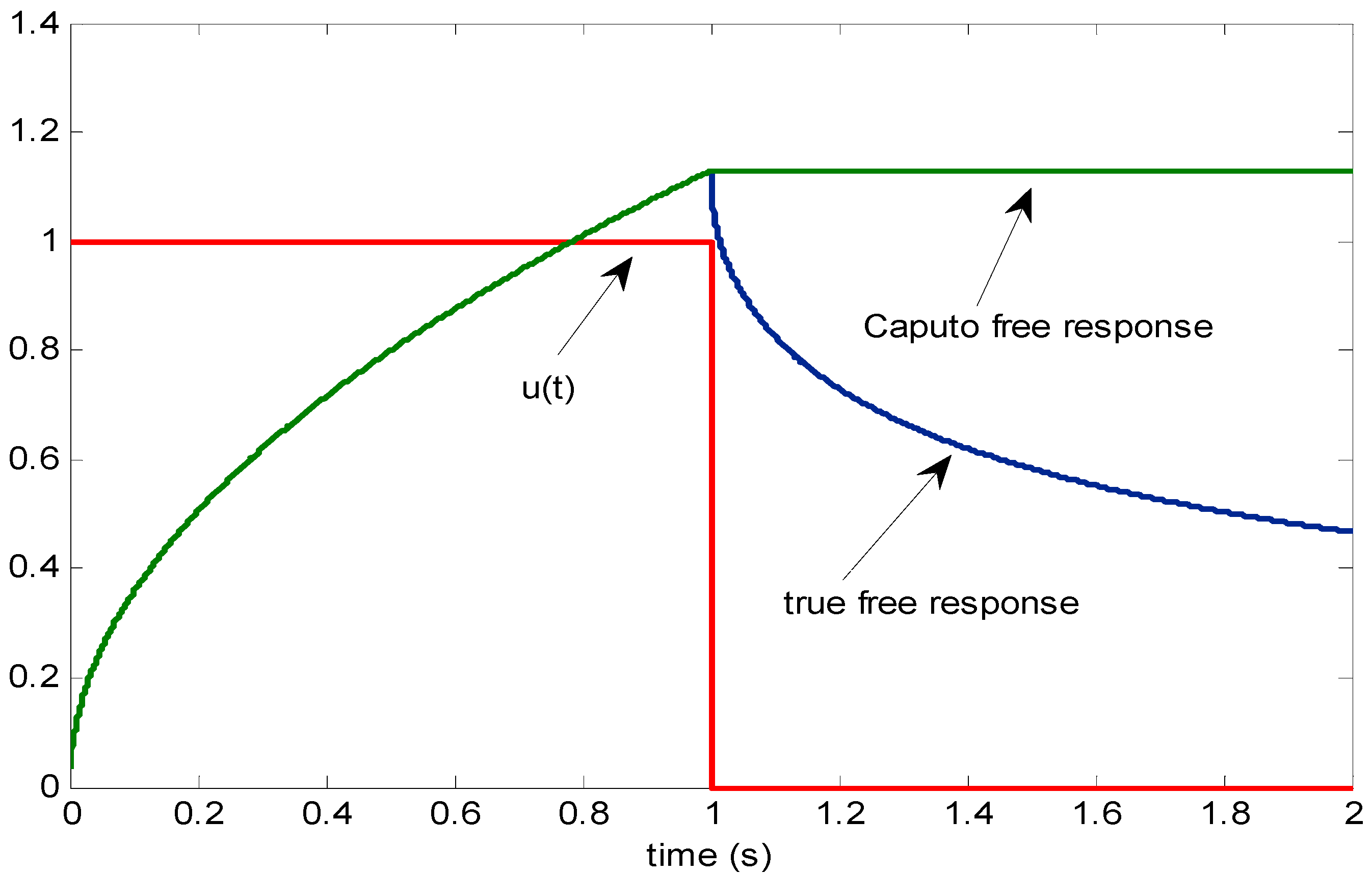
The integration of FDE/FDS based on the Caputo derivative definition (or on the Riemann–Liouville derivative) are wrong approaches leading to erroneous free responses.

-

The frequency-distributed state-space model provides the exact expression of the free response using the usual tools of linear system theory. Consequently, this distributed model is the necessary tool to express transients of the fractional integrator and thus those of FDE/FDS.

Notice that the Grünwald–Letnikov approach based on relation (25) provides a correct solution to the integration of FDE/FDS. However, its initial conditions, composed of past values of $x(-i)$ since $k=-\infty$, are not easy to use, particularly for an initialization objective.

5.6. The Caputo Derivative Definition Revisited

We have demonstrated with the previous elementary counter example that the integration technique based on the Caputo derivative definition is unable to provide a correct expression of the free response of an elementary initial-value problem. Of course, we have pointed out the reason of this failure, i.e., $x(0)$ does not represent the initial condition of the fractional integrator. Basically, what is the origin of this error?

In order to understand why so many researchers have been misled by the so-called “initial condition”$x(0)$, we have to once again consider the definition (12) of the Caputo derivative:

$${}^{C}D_t^n\left(x(t)\right)=I_t^{1-n}\left(\frac{dx(t)}{dt}\right)$$

This derivative relies on a fractional integrator $\frac{1}{s^{1-n}}$, so we have to take into account its internal state variables $z_C(\omega ,t)$ at $t=0$ (notice that $z_C(\omega ,t)\ne z(\omega ,t)$) [34].

Thus, the distributed-frequency model of the Caputo derivative corresponds to that of the fractional integrator $I_t^{1-n}\left(.\right)$, where, in this case, the input and the output are $\frac{dx(t)}{dt}$ and ${}^{C}D_t^n\left(x(t)\right)$, respectively:

$$\left\{\begin{array}{c}\frac{\partial z_C(\omega ,t)}{\partial t}=-\omega z_C(\omega ,t)+\frac{dx(t)}{dt}\hspace{1em}\omega \left[0,\infty \right)\\ {}^{C}D_t^n\left(x(t)\right)={\displaystyle \underset{0}{\overset{\infty }{\int }}{\mu }_{1-n}(\omega )z_C(\omega ,t)d\omega }\\ {\mu }_{1-n}(\omega )=\frac{\sin \left((1-n)\pi \right)}{\pi }{\omega }^{-(1-n)}\hspace{1em}\mathrm{and}\hspace{1em}0<n<1\end{array}\right.$$

(40)

with the initial condition $z_C(\omega ,0)$ $\mathrm{and} \omega \in \left[0,\infty \right)$.

By using the Laplace transform, we can write

$$\left\{\begin{array}{c}{Z}_C(\omega ,s)=\frac{z_C(\omega ,0)}{s+\omega }+\frac{L\left\{\frac{dx(t)}{dt}\right\}}{s+\omega }\hspace{1em}\omega \in \left[0,\infty \right)\\ \mathrm{with} L\left\{\frac{dx(t)}{dt}\right\}=sX(s)-x(0)\end{array}\right.$$

Thus, we obtain

$$L\left\{{}^{C}D_t^n\left(x(t)\right)\right\}={\displaystyle \underset{0}{\overset{\infty }{\int }}}{\mu }_{1-n}(\omega )Z_C(\omega ,s)d\omega =s^{n}X(s)-\frac{x(0)}{s^{1-n}}+{\displaystyle \underset{0}{\overset{\infty }{\int }}\frac{{\mu }_{1-n}(\omega )}{s+\omega }}{z}_C(\omega ,0)d\omega$$

(41)

We can conclude that the usual initial condition of the Caputo derivative is wrong because it does not take into account the transients of its associated integrator $\frac{1}{s^{1-n}}$, i.e., its distributed initial conditions $z_C(\omega ,0)$.

Notice that the same conclusions apply to the Riemann–Liouville derivative [34].

Consequently, the Caputo derivative approach to the integration of FDE/FDS must be rejected because it provides wrong solutions to fractional initial-value problems. This approach is wrong for two main reasons:

-

The exact initial conditions of the Caputo derivative are $x(0)$ and the distributed state variable initial condition $z_C(\omega ,0)$.

-

The technique based on the Caputo derivative is not natural because the true and physical initial conditions are those of the fractional integrator $\frac{1}{s^n}$ of Equation (30), i.e., $z(\omega ,0)$, such as in the integer order case.

Numerical simulations of the Caputo and Riemann–Liouville derivatives exhibiting the role of their initial conditions are available in [38] and in Volume 1 of [34].

6. Fractional Differential Systems Transients

6.1. Integration of a FDE

We demonstrated in the previous section that it is necessary to use the frequency-distributed model of the fractional integrator to take into account the transients of the free response. Thus, we have to apply the same approach for the integration of any FDE/FDS initial value problem (6,7). As we have shown, the solution is provided by the fractional integral equation, which is equivalent to the integer order case (2):

$$x(t)=I_t^n\left(f\left(x(t),u(t)\right)\right)+x_0(t),$$

(42)

where $x_0(t)$ is the initialization function of the Riemann–Liouville integral

$$x_0(t)={\displaystyle \underset{0}{\overset{\infty }{\int }}{\mu }_n(\omega )z(\omega ,0)e^{-\omega t}d\omega }.$$

(43)

Notice that (42) is a Volterra integral equation.

Fundamentally, Figure 3 displays the graphical representation of the integral Equation (42), which underlines the closed-loop behavior of the FDE/FDS based on the fractional integrator $\frac{1}{s^n}$ with the initialization function $x_0\left(\mathrm{t}\right)$.

However, we can also use the frequency-distributed model of the fractional integrator, where its input is $v(t)=D^n\left(x(t)\right)=f\left(x(t),u(t)\right)$, which leads to the distributed representation of the FDE:

$$\left\{\begin{array}{c}\frac{\partial z(\omega ,t)}{\partial t}=-\omega z(\omega ,t)+f\left(x(t),u(t)\right)\\ x(t)={\displaystyle \underset{0}{\overset{\infty }{\int }}{\mu }_n(\omega )z(\omega ,t)d\omega }\\ \mu (\omega )=\frac{\sin (n\pi )}{\pi }{\omega }^{-n}\hspace{1em}0<n<1\end{array}\right.$$

(44)

In this case, the solution $z(\omega ,t)$ is provided by the distributed integer-order integral equation:

$$\begin{array}{lll}\hfill z(\mathsf{\omega },t)& ={\displaystyle \underset{0}{\overset{t}{\int }}\left[-\mathsf{\omega }z(\mathsf{\omega },t)+f\left(x(\mathsf{\tau }),u(\mathsf{\tau })\right)\right]d\mathsf{\tau }+z(\mathsf{\omega },0)}\hfill & \forall \mathsf{\omega }\in \left[0,\infty \right)\\ & =I_t^1\left(-\mathsf{\omega }z(\mathsf{\omega },t)+f\left(x(t),u(t)\right)\right)+z(\mathsf{\omega },0)\hfill & \end{array}$$

(45)

where $z(\omega ,0)$ is the initial condition of the integer order integral.

We can represent (see Figure 4) this frequency distributed system graphically, where frequency varies from $\omega =0$ to $\omega =+\infty$, according to its Laplace transform. This graph corresponds to Figure 3, where the fractional integrator is replaced by its distributed graph of Figure 1.

Equations (42) and (43) and the graph of Figure 3 focus on the pseudo-state variable $x(t)$, whereas Equation (44) and the graph of Figure 4 focus on the internal state variables $z(\omega ,t)$ of the integrator, which are in fact those of the FDE/FDS.

Notice that, for the isolated integrator (Figure 1), with input $v(t)$ and output $x(t)$, the state variables are decoupled and evolve independently. On the other hand, in system (44), i.e., in the graph of Figure 4, the state variables are coupled by the relation $v(t)=f\left(x(t),u(t)\right)$. This means that the evolution of the state variable $z(\omega ,t)$ (for the particular value) depends on all the other state variables $z(\xi ,t)\hspace{1em}\xi \in \left[0,\infty \right)$. Namely, the original FDE/FDS (6) has been transformed into an infinite-dimension system of first-order differential Equations (44).

These are the two “faces” of the same problem:

-

Equation (42) and Figure 3 correspond to the pseudo-state variable $x(t)$, directly taking into account the fractional order n.

-

Equation (44) and Figure 4 correspond to the system of distributed state variables $z(\omega ,t)$, whose solution is obtained through an integer-order approach. The pseudo-state variable $x(t)$ is provided by a weighted integral, where ${\mu }_n(\omega )$ is the link between the integer order and fractional order domains.

In Figure 3 and Figure 4, there is no hypothesis about the nature of $f\left(x(t),u(t)\right)$ which can be either linear or nonlinear. In the nonlinear case, the integral formulation of the FDE/FDS initial-value problem leads to (42) or (45). The solution of these integral equations can be obtained with Picard’s method, which is currently used to solve nonlinear fractional order problems (see for instance [3]).

Of course, the nonlinear case is a very wide topic, and our objective is not to treat it in this paper. In fact, the linear case is also of fundamental interest, and we propose to revisit it, essentially to formulate free responses.

6.2. FDS Transients and the Mittag–Leffler Function

First, we consider the elementary FDE initial-value problem:

$$\begin{array}{cc}{D}^n\left(x(t)\right)=ax(t)& 0<n<1\end{array}$$

(46)

with the distributed initial condition $z(\mathsf{\omega },0)\hspace{1em}\forall \mathsf{\omega }\in \left[0,\infty \right)$.

System (46) can be transformed into the distributed frequency one:

$$\left\{\begin{array}{c}\frac{\partial z(\mathsf{\omega },t)}{\partial t}=-\mathsf{\omega }z(\mathsf{\omega },t)+ax(t)\\ x(t)={\displaystyle \underset{0}{\overset{\infty }{\int }}{\mathsf{\mu }}_n(\mathsf{\omega })z(\mathsf{\omega },t)d\mathsf{\omega }}\end{array}\right.$$

(47)

with the initial condition $z(\mathsf{\omega },0)$.

Using the Laplace transform, we can write

$$sZ(\omega ,s)-z(\omega ,0)=-\omega Z(\omega ,s)+aX(s),$$

i.e., $\mathrm{X}(s)=\frac{s^n}{s^n-a}{\displaystyle \underset{0}{\overset{\infty }{\int }}{\mu }_n(\omega )\frac{z(\omega ,0)}{s+\omega }}d\omega$

$$\mathrm{or} \mathrm{X}(s)=s\frac{s^{n-1}}{s^n-a}{X}_0(s),$$

(48)

with $X_0(s)={\displaystyle \underset{0}{\overset{\infty }{\int }}{\mu }_n(\omega )\frac{z(\omega ,0)}{s+\omega }d\omega }$

So,

$$x_0(t)=L^{-1}\left\{{\displaystyle \underset{0}{\overset{\infty }{\int }}{\mathsf{\mu }}_n(\mathsf{\omega })\frac{z(\mathsf{\omega },0)}{s+\mathsf{\omega }}d\mathsf{\omega }}\right\}={\displaystyle \underset{0}{\overset{\infty }{\int }}{\mathsf{\mu }}_n(\mathsf{\omega })z(\mathsf{\omega },0)e^{-\mathsf{\omega }t}d\mathsf{\omega }}$$

(49)

Let us remember that

$$L\left\{E_{n,1}\left(a{t}^n\right)\right\}=\frac{s^{n-1}}{s^n-a}$$

(50)

where $E_{n,1}\left(a{t}^n\right)$ is the Mittag–Leffler function:

$$E_{n,1}\left(a{t}^n\right)={\displaystyle \sum _{k=0}^{\infty }\frac{{\left(a{t}^n\right)}^k}{\Gamma (nk+1)}},$$

(51)

which is the generalization of the exponential function, since for $n=1$ we obtain $E_{1,1}\left(a{t}^1\right)={\displaystyle \sum _{k=0}^{\infty }\frac{{\left(a{t}^1\right)}^k}{k!}}=e^{at}$.

Consequently, we obtain

$$x(t)=L^{-1}\left\{X(s)\right\}=\frac{d}{dt}\left\{E_{n,1}\left(a{t}^n\right)\ast x_0(t)\right\}.$$

(52)

We can easily generalize this result to any linear FDS initial value problem:

$$D^n\left(\underset{¯}{x}(t)\right)=A\underset{¯}{x}(t)+\underset{¯}{B}u(t)\hspace{1em}0<n<1,$$

(53)

with the distributed initial condition $\underset{¯}{z}(\omega ,0)\hspace{1em}\forall \omega \in \left[0,\infty \right)$.

Defining the matrix Mittag–Leffler function:

$$E_{n,1}\left(A{t}^n\right)={\displaystyle \sum _{k=0}^{\infty }\frac{{\left(A{t}^n\right)}^k}{\mathsf{\Gamma }(nk+1)}},$$

(54)

we can write

$$\underset{¯}{x}(t)=\frac{d}{dt}\left\{E_{n,1}\left(A{t}^n\right)\ast {\underset{¯}{x}}_0(t)\right\}+{\displaystyle \underset{0}{\overset{t}{\int }}{E}_{n,1}\left(A{(t-\tau )}^n\right)}\underset{¯}{B}\tilde{u}(\tau )d\tau ,$$

(55)

where $\tilde{u}(\mathsf{\tau })=D^{1-n}\left(u(\tau )\right)$ and ${\underset{¯}{x}}_0(t)={\displaystyle \underset{0}{\overset{\infty }{\int }}{\mu }_n(\omega )\underset{¯}{z}(\omega ,0)e^{-\omega t}d\omega }$.

Obviously, the free response $\frac{d}{dt}\left\{E_{n,1}\left(A{t}^n\right)\ast {\underset{¯}{x}}_0(t)\right\}$ of $\underset{¯}{x}(t)$ is more complex than the wrong usual one derived from (8), i.e., $\underset{¯}{x}(t)=E_{n,1}\left(A{t}^n\right)\underset{¯}{x}(0)$.

Moreover, there is a major difficulty, i.e., the convolution between the Mittag–Leffler function and $x_0(t)$, which is not a straightforward operation. Thus, the interest of this expression is essentially theoretical.

Notice also that the matrix Mittag–Leffler function does not verify the semi-group properties of the matrix exponential function [53,54].

Remark 4:

The use of the Caputo derivative is based on the assumption $x_0(t)=x(0)=cte\hspace{1em}\forall t$. Is this requirement always wrong? In addition, if it is correct, what does it mean?

Consider the following system

$$D^n\left(x(t)\right)=ax(t)+bu(t)\hspace{1em}0<n<1$$

and suppose that it is at rest at t = 0 and that $u(t)=UH(t)$.

Since, in this case,

$Z(\omega ,s)=\frac{aX(s)+b\frac{U}{s}}{s+\omega }$ and $\mathrm{X}(s)={\displaystyle \underset{0}{\overset{\infty }{\int }}{\mu }_n(\omega )Z(\omega ,s)d\omega }$, we obtain $Z(\mathsf{\omega },s)=b\frac{s^n}{s^n-a}\frac{1}{s+\mathsf{\omega }}\frac{U}{s}$.

Thus

$$z(\omega ,\infty )=\underset{s\to 0}{\lim sZ(\omega ,s)}=0\hspace{1em}\forall \omega \ne 0 \mathrm{and} z(0,\infty )=\underset{s\to 0}{\lim }\hspace{0.33em}\frac{bU}{s^{1-n}}=\infty$$

(56)

On the other hand, we can also write $x(\infty )=-\frac{b}{a}U$ for a stable system, i.e., a < 0 in our case.

Assume that we have applied the same step input $UH(t)$, but, at $t=-\infty$, this means that at t = 0, we obtained $x(0)=-\frac{b}{a}U$ for a long time in the past (t < 0).

Consequently, the condition $x_0(t)=x(0)=cte\hspace{1em}\forall t$ requires that the system has been at rest for a very long time.

Then

$$x_0(t)={\displaystyle \underset{0}{\overset{\infty }{\int }}{\mathsf{\mu }}_n(\mathsf{\omega })z(\mathsf{\omega },0)e^{-\mathsf{\omega }t}d\mathsf{\omega }}={\displaystyle \underset{0}{\overset{\infty }{\int }}{\mathsf{\mu }}_n(\mathsf{\omega })z(0,0)e^{-0t}d\mathsf{\omega }}=x(0)=cte.$$

(57)

Since $z(\mathsf{\omega },\infty )\hspace{1em}=0\forall \mathsf{\omega }\ne 0$.

Theoretically, the condition $x_0(t)=x(0)=cte\hspace{1em}\forall t$ can be achieved, but it is completely unrealistic. Moreover, it would require infinite energy [34].

Remark 5:

Consider again the revisited definition of the Caputo derivative (see Section 5.6):

$${}^{C}D_t^n\left(x(t)\right)=I_t^{1-n}\left(\frac{dx(t)}{dt}\right)\Rightarrow \left\{\begin{array}{c}\frac{\partial z_C(\omega ,t)}{\partial t}=-\omega z_C(\omega ,t)+\frac{dx(t)}{dt}\hspace{1em}\omega \in \left[0,\infty \right)\\ {}^{C}D_t^n\left(x(t)\right)={\displaystyle \underset{0}{\overset{\infty }{\int }}{\mu }_{1-n}(\omega )z_C(\omega ,t)d\omega }\\ {\mu }_{1-n}(\omega )=\frac{\sin \left((1-n)\pi \right)}{\pi }{\omega }^{-(1-n)} and 0<n<1\end{array}\right.$$

with $z_C(\omega ,t)=z_C(\omega ,0) \mathrm{at} t=0$.

We have demonstrated (41) that:

$$L\left\{{}^{C}D_t^n\left(x(t)\right)\right\}=s^{n}X(s)-\frac{x(0)}{s^{1-n}}+{\displaystyle \underset{0}{\overset{\infty }{\int }}\frac{{\mathsf{\mu }}_{1-n}(\omega )}{s+\mathsf{\omega }}}{z}_C(\mathsf{\omega },0)d\mathsf{\omega }.$$

If $x(t)=cte$, for a long time in the past (t < 0), then $\frac{dx(t)}{dt}=0$. This means that $z_C(\mathsf{\omega },t)=0\hspace{1em}\forall \mathsf{\omega }$ for a long time in the past (t < 0), and consequently $z_C(\mathsf{\omega },0)=0\hspace{1em}\forall \mathsf{\omega }$.

Then, we can write $L\left\{{}^{C}D_t^n\left(x(t)\right)\right\}=s^{n}X(s)-\frac{x(0)}{s^{1-n}}$.

Obviously, the previous conditions are very restrictive, and the usual initial condition is wrong as soon as there is a variation of x(t).

Remark 6:

We have demonstrated (52) that:

$$x(t)=\frac{d}{dt}\left\{E_{n,1}\left(a{t}^n\right)\ast x_0(t)\right\}=E_{n,1}\left(a{t}^n\right)\ast \frac{d}{dt}{x}_0(t)$$

Since $x_0(t)=x(0)=cte\hspace{1em}\forall t$, we can write $x_0(t)=x(0)H(t)$, so $\frac{d}{dt}{x}_0(t)=x(0)\delta (t)$.

Then,

$$x(t)=E_{n,1}\left(a{t}^n\right)\ast x(0)\delta (t)=E_{n,1}\left(a{t}^n\right)x(0)$$

(58)

is the usual result corresponding to the Caputo derivative assumption.

The conclusion is that many results obtained with the Caputo derivative approach are not necessarily wrong, but they require the previous very restrictive assumptions related to $x(0)$.

6.3. FDS Transients Expressed with the Distributed Exponential Function

Previously, the problem of fractional transients has been focused on the pseudo-state variable dynamics, with no insight in the distributed state variable. So, we propose now to express the dynamics of $z(\mathsf{\omega },t)$. Let us start again with the elementary system (46):

$$D^n\left(x(t)\right)=ax(t)\hspace{1em}0<n<1$$

with the distributed initial condition $z(\mathsf{\omega },0)\hspace{1em}\forall \mathsf{\omega }\in \left[0,\infty \right)$.

The corresponding distributed frequency model (47) leads to:

$$\frac{\partial z(\mathsf{\omega },t)}{\partial t}=-\mathsf{\omega }z(\mathsf{\omega },t)+a{\displaystyle \underset{0}{\overset{\infty }{\int }}{\mathsf{\mu }}_n(\mathsf{\xi })z(\mathsf{\xi },t)d\mathsf{\xi }}\hspace{1em}\forall \mathsf{\omega }\in \left[0,\infty \right).$$

(59)

Notice that we have to separate the current frequency $\mathsf{\omega }$ from all the other ones $\mathsf{\xi }\in \left[0,\infty \right).$ This means that the behavior of $z(\mathsf{\omega },t)$ depends on all the behaviors of the other state variables $z(\mathsf{\xi },t)$.

Let us define $\mathsf{\delta }(\mathsf{\xi })$, which is the frequency Dirac impulse verifying ${\displaystyle \underset{0}{\overset{\infty }{\int }}\mathsf{\delta }(\mathsf{\xi })d\mathsf{\xi }=1}$.

Then,

$${\displaystyle \underset{0}{\overset{\infty }{\int }}\mathsf{\omega }\mathsf{\delta }(\mathsf{\xi }-\mathsf{\omega })z(\mathsf{\xi },t)d\mathsf{\xi }=\mathsf{\omega }{\displaystyle \underset{0}{\overset{\infty }{\int }}\mathsf{\delta }(\mathsf{\xi }-\mathsf{\omega })z(\mathsf{\xi },t)d\mathsf{\xi }=\mathsf{\omega }}}z(\mathsf{\omega },t).$$

(60)

Let us define

$$\mathsf{\psi }(\mathsf{\omega },\mathsf{\xi })=-\mathsf{\omega }\mathsf{\delta }(\mathsf{\xi }-\mathsf{\omega })+a{\mathsf{\mu }}_n(\mathsf{\xi })$$

(61)

Then, (59) can be expressed as:

$$\frac{\partial z(\mathsf{\omega },t)}{\partial t}=-\mathsf{\omega }{\displaystyle \underset{0}{\overset{\infty }{\int }}\mathsf{\delta }(\mathsf{\xi }-\mathsf{\omega })z(\mathsf{\xi },t)d\mathsf{\xi }}+a{\displaystyle \underset{0}{\overset{\infty }{\int }}{\mathsf{\mu }}_n(\mathsf{\xi })z(\mathsf{\xi },t)d\mathsf{\xi }}={\displaystyle \underset{0}{\overset{\infty }{\int }}\mathsf{\psi }(\mathsf{\omega },\mathsf{\xi })z(\mathsf{\xi },t)d\mathsf{\xi }}$$

(62)

The solution $z(\mathsf{\omega },t)$ requires the integration of the integer-order distributed system (59) with the initial condition $z(\mathsf{\omega },0)\hspace{1em}\forall \mathsf{\omega }\in \left[0,\infty \right)$. Basically, the solution verifies the integral relation:

$$\begin{array}{ll}\hfill z(\omega ,t)& ={\displaystyle \underset{0}{\overset{t}{\int }}\left[{\displaystyle \underset{0}{\overset{\infty }{\int }}\mathsf{\Psi }(\omega ,\xi )z(\xi ,\tau )d\xi }\right]d\tau +z(\omega ,0)}\hfill \\ & ={}_{0}I_t^1\left[{\displaystyle \underset{0}{\overset{\infty }{\int }}\mathsf{\Psi }(\omega ,\xi )z(\xi ,\tau )d\xi }\right]+z(\omega ,0)\hspace{1em}\omega \in \left[0,\infty \right)\end{array}$$

(63)

This integration is performed with Picard’s method, which is an iterative technique (3).

At the first iteration, $z(\mathsf{\omega },t)$ is approximated by $z(\mathsf{\omega },0)$.

Since $z(\mathsf{\omega },0)$ and ${\displaystyle \underset{0}{\overset{\infty }{\int }}\mathsf{\psi }(\mathsf{\omega },\mathsf{\xi })d\mathsf{\xi }}$ are constants for ${}_{0}I_t^1$, we obtain

$$z_1(\omega ,t)=z(\omega ,0)+{}_{0}I_t^1\left[{\displaystyle \underset{0}{\overset{\infty }{\int }}\psi (\omega ,\xi )z(\omega ,0)d\xi }\right]=z(\omega ,0)+z(\omega ,0)t{\displaystyle \underset{0}{\overset{\infty }{\int }}\psi (\omega ,\xi )d\xi }.$$

(64)

At the second iteration, $z(\mathsf{\omega },t)$ is approximated by $z_1(\mathsf{\omega },t)$. So, we obtain

$$z_2(\mathsf{\omega },t)=z(\mathsf{\omega },0)+z(\mathsf{\omega },0)t{\displaystyle \underset{0}{\overset{\infty }{\int }}\mathsf{\psi }(\mathsf{\omega },\mathsf{\xi })d\mathsf{\xi }}+z(\mathsf{\omega },0)\frac{t^2}{2}{\left[{\displaystyle \underset{0}{\overset{\infty }{\int }}\mathsf{\psi }(\mathsf{\omega },\mathsf{\xi })d\mathsf{\xi }}\right]}^2$$

(65)

Additionally, at iteration k, we obtain

$$z_k(\mathsf{\omega },t)={\displaystyle \sum _{j=0}^k\frac{t^j}{j!}}{\left[{\displaystyle \underset{0}{\overset{\infty }{\int }}\mathsf{\psi }(\mathsf{\omega },\mathsf{\xi })d\mathsf{\xi }}\right]}^{j}z(\mathsf{\omega },0)$$

(66)

$$\mathrm{Thus}, z(\mathsf{\omega },t)=\underset{k\to \infty }{\lim }{\displaystyle \sum _{j=0}^k\frac{t^j}{j!}}{\left[{\displaystyle \underset{0}{\overset{\infty }{\int }}\mathsf{\psi }(\mathsf{\omega },\mathsf{\xi })d\mathsf{\xi }}\right]}^{j}z(\mathsf{\omega },0),$$

(67)

$$\mathrm{i}.\mathrm{e}., z(\mathsf{\omega },t)=\left[{\displaystyle \sum _{k=0}^{\infty }\frac{t^k}{k!}}{\left[{\displaystyle \underset{0}{\overset{\infty }{\int }}\mathsf{\psi }(\mathsf{\omega },\mathsf{\xi })d\mathsf{\xi }}\right]}^k\right]z(\mathsf{\omega },0)$$

(68)

Notice that, in the integer order case, $\frac{dx(t)}{dt}=ax(t)$, so $\mathsf{\psi }(\mathsf{\omega },\mathsf{\xi })\equiv a$.

$$\mathrm{Then}, x(t)=\left[{\displaystyle \sum _{k=0}^{\infty }{a}^k\frac{t^k}{k!}}\right]x(0)=e^{at}x(0).$$

(69)

Thus, in the distributed case, we can define the distributed exponential function:

$$\mathsf{\varphi }(t)=\exp \left(t{\displaystyle \underset{0}{\overset{\infty }{\int }}\mathsf{\psi }(\mathsf{\omega },\mathsf{\xi })d\mathsf{\xi }}\right)={\displaystyle \sum _{k=0}^{\infty }\frac{t^k}{k!}}{\left[{\displaystyle \underset{0}{\overset{\infty }{\int }}\mathsf{\psi }(\mathsf{\omega },\mathsf{\xi })d\mathsf{\xi }}\right]}^k$$

(70)

and

$$z(\mathsf{\omega },t)=\exp \left(t{\displaystyle \underset{0}{\overset{\infty }{\int }}\mathsf{\psi }(\mathsf{\omega },\mathsf{\xi })d\mathsf{\xi }}\right)z(\mathsf{\omega },0)=\mathsf{\varphi }(t)z(\mathsf{\omega },0)\hspace{1em}\mathsf{\omega }\in \left[0,\infty \right),$$

(71)

which is the distributed generalization of Equation (69).

Then, we can generalize the distributed exponential to the linear multidimensional non-commensurate order case:

$$D^{\underset{¯}{n}}\left(\underset{¯}{x}(t)\right)=A\underset{¯}{x}(t) \dim \left(\underset{¯}{x}(t)\right)=N,$$

(72)

where ${\underset{¯}{n}}^T=\left[n_1\dots n_i\dots n_N\right]\hspace{1em}0<n_i\le 1$.

Moreover, $0<n_i\le 1$ means that the FDS system may include integer-order derivatives, since, with real systems, the dynamics are caused either by integer-order or fractional-order derivatives.

So, (72) corresponds to the integer-order frequency-distributed differential system:

$$\left\{\begin{array}{cc}\hfill \frac{\partial \underset{¯}{z}(\omega ,t)}{\partial t}=-\omega \underset{¯}{z}(\omega ,t)+A{\displaystyle \underset{0}{\overset{\infty }{\int }}\left[{\mu }_{\underset{¯}{n}}(\xi )\right]}\underset{¯}{z}(\xi ,t)d\xi & \dim \left(\underset{¯}{z}(t)\right)=N\hfill \\ \hfill \underset{¯}{x}(t)={\displaystyle \underset{0}{\overset{\infty }{\int }}\left[{\mu }_{\underset{¯}{n}}(\xi )\right]}\underset{¯}{z}(\xi ,t)d\xi & \end{array}\right.$$

(73)

with the initial condition $\underset{¯}{z}(\omega ,0)\hspace{1em}\forall \omega \in \left[0,\infty \right)$,

$$\mathrm{and} \left[{\mu }_{\underset{¯}{n}}(\xi )\right]=\left[\begin{array}{ccc}{\mu }_{n_1}(\xi )& & 0\\ & {\mu }_{n_i}(\xi )& \\ 0& & {\mu }_{n_N}(\xi )\end{array}\right]$$

(74)

Let us define the matrix

$$\mathsf{\Psi }(\mathsf{\omega },\mathsf{\xi })=-\mathsf{\omega }\mathsf{\delta }(\mathsf{\xi }-\mathsf{\omega })I+A\left[{\mathsf{\mu }}_{\underset{¯}{n}}(\mathsf{\xi })\right]$$

(75)

where I is the Identity matrix with appropriate dimension.

Then, the differential system (73) can be expressed as

$$\frac{\partial \underset{¯}{z}(\omega ,t)}{\partial t}={\displaystyle \underset{0}{\overset{\infty }{\int }}\mathsf{\Psi }(\omega ,\xi )\underset{¯}{z}}(\xi ,t).$$

(76)

Therefore, the distributed exponential $\exp \left(t{\displaystyle \underset{0}{\overset{\infty }{\int }}\mathsf{\psi }(\mathsf{\omega },\mathsf{\xi })d\mathsf{\xi }}\right)$ function is replaced by the distributed exponential matrix:

$$\mathsf{\Phi }(t)=\exp \left(t{\displaystyle \underset{0}{\overset{\infty }{\int }}\mathsf{\Psi }(\mathsf{\omega },\mathsf{\xi })d\mathsf{\xi }}\right)={\displaystyle \sum _{k=0}^{\infty }\frac{t^k}{k!}}{\left[{\displaystyle \underset{0}{\overset{\infty }{\int }}\mathsf{\Psi }(\mathsf{\omega },\mathsf{\xi })d\mathsf{\xi }}\right]}^k,$$

(77)

and the solution of (76) is:

$$\underset{¯}{z}(\omega ,t)=\exp \left(t{\displaystyle \underset{0}{\overset{\infty }{\int }}\mathsf{\Psi }(\omega ,\xi )d\xi }\right)\underset{¯}{z}(\omega ,0)=\mathsf{\Phi }(t)\underset{¯}{z}(\omega ,0)\hspace{1em}\omega \in \left[0,\infty \right).$$

(78)

Notice that, contrary to the Mittag–Leffler matrix, the distributed exponential matrix shares the same semi-group properties (see chapter 2 of [54]) as its integer order analog, i.e.,

$$\mathsf{\Phi }(t,t_0)=\mathsf{\Phi }(t,\mathsf{\tau })\mathsf{\Phi }(\mathsf{\tau },t_0)\hspace{1em}{t}_0<\mathsf{\tau }<t$$

(79)

Finally, the solution of the linear multidimensional non-commensurate order FDS (72) with the initial condition $\underset{¯}{z}(\omega ,0)\hspace{1em}\forall \omega \in \left[0,\infty \right)$ is similar to the integer-order case (5), i.e.,

$$\underset{¯}{z}(\omega ,t)=\mathsf{\Phi }(t)\underset{¯}{z}(\omega ,0)+{\displaystyle \underset{0}{\overset{t}{\int }}}\mathsf{\Phi }(t-\tau )\underset{¯}{B}u(\tau )d\tau \hspace{1em}\omega \in \left[0,\infty \right),$$

(80)

where $\mathsf{\Phi }(t)$ is the distributed exponential transition matrix.

6.4. Computation of the Distributed Exponential Function

The interest of the distributed exponential function, either in scalar or matrix form, is essentially theoretical. Practically, in order to compute it, the distributed exponential function requires frequency discretization, i.e., a discretization of the continuous distributed integrator model:

$$\left\{\begin{array}{c}\frac{\partial z(\omega ,t)}{\partial t}=-\omega z(\omega ,t)+v(t)\hspace{1em}\omega \in \left[0,\infty \right)\\ x(t)={\displaystyle \underset{0}{\overset{\infty }{\int }}\mu (\omega )z(\omega ,t)d\omega }\end{array}\right.$$

(81)

Direct discretization is possible, but indirect discretization is more efficient [34,35]. It is based on the approximation of the frequency response of $\frac{1}{s^n} 0<n<1$, on a frequency interval $\left[{\mathsf{\omega }}_{\min },{\mathsf{\omega }}_{\max }\right]$ with J first-order cells, associated with an integer-order integrator at =0. So, the global model is composed of J + 1 cells (or modes) such as:

$$\left\{\begin{array}{c}\frac{d{z}_j(t)}{dt}=-{\omega }_j{z}_j(t)+v(t)\hspace{1em}j=0 to J\\ x(t)={\displaystyle \sum _{j=0}^J{c}_j{z}_j(t)}\end{array}\right.$$

(82)

and the elementary system $D^n\left(x(t)\right)=ax(t)$ becomes:

$$\left\{\begin{array}{c}\frac{d{z}_j(t)}{dt}=-{\mathsf{\omega }}_j{z}_j(t)+a{\displaystyle \sum _{j=0}^J{c}_j{z}_j(t)}\hspace{1em}j=0 to J\\ x(t)={\displaystyle \sum _{j=0}^J{c}_j{z}_j(t)}\end{array}\right.$$

(83)

where ${\mathsf{\omega }}_j$ varies from ${\mathsf{\omega }}_0=0$ to ${\mathsf{\omega }}_J$.

Let us define:

$$\begin{array}{lll}{\underset{¯}{z}}_I^T(t)=\left[z_0(t)\dots z_j(t)\dots z_J(t)\right]\hfill & \dim \left({\underset{¯}{z}}_I\right)=J+1\hfill & \\ A_I=\left[\begin{array}{ccc}-{\omega }_0& & \\ & -{\omega }_j& \\ & & -{\omega }_J\end{array}\right]\hfill & {\underset{¯}{B}}_I^T=\left[1\dots 1\dots 1\right]\hfill & {\underset{¯}{C}}_I=\left[c_0\dots c_j\dots c_J\right]\hfill \end{array}$$

(84)

Then, the previous system (83) is transformed into the following one

$$\left\{\begin{array}{c}\frac{d{\underset{¯}{z}}_I(t)}{dt}=A_I{\underset{¯}{z}}_I(t)+a{\underset{¯}{B}}_I{\underset{¯}{C}}_I{\underset{¯}{z}}_I(t)=A_{syst}{\underset{¯}{z}}_I(t)\\ x(t)={\underset{¯}{C}}_I{\underset{¯}{z}}_I(t)\end{array}\right. \mathrm{with} A_{syst}=A_I+a\underset{¯}{B_I}\underset{¯}{C_I}$$

(85)

Thus, the solution of system (85) with the initial condition ${\underset{¯}{z}}_I^T(0)=\left[z_0(0)\dots z_j(0)\dots z_J(0)\right]$ is expressed as

$$\underset{¯}{Z}(t)=e^{A_{syst}t}\underset{¯}{Z}(0)={\mathsf{\varphi }}_d(t)\underset{¯}{Z}(0),$$

(86)

where ${\mathsf{\varphi }}_d(t)=e^{A_{syst}t}$ is the matrix exponential corresponding to the frequency discretization of the distributed exponential function $\mathsf{\varphi }(t)=\exp \left(t{\displaystyle \underset{0}{\overset{\infty }{\int }}\mathsf{\psi }(\mathsf{\omega },\mathsf{\xi })d\mathsf{\xi }}\right)$.

Numerical examples of the distributed exponential function are available in chapter 9 volume 1 of [34].

7. Conclusions

In this paper, it has been proved, thanks to an elementary counter example, that the solution of the FDE initial value problem cannot be provided by the well-known Caputo derivative approach. The origin of this error relies on ignoring the dynamics of the fractional integrator, which has caused confusion between pseudo initial conditions of the Caputo derivative and the initialization function of the Riemann–Liouville integral.

Furthermore, it has been demonstrated that it is necessary to take into account two complementary models of the fractional integrator: the classical model used to express the pseudo state variable $x(t)$ is an input/output model, whereas the distributed model is an infinite-dimension state variable model, which is adapted to the formulation of free responses thanks to the initial values of its distributed state variable $z(\omega ,t)$, as proved by the counter-example.

These two models of the fractional integrator generate two complementary approaches to the modeling of FDE and FDS one being focused on the pseudo-state variable, whereas the other permits to express internal transients linked to the distributed state variable. Two expressions of their free responses have been formulated in the linear case, one with the help of a convolution of the Mittag–Leffler function with the initialization function, and the other thanks to the definition of a distributed exponential function, which is a straightforward generalization of the integer-order case.

Beyond the misuse of fractional derivatives to solve the initial-value problem, the main conclusion of this paper is that any fractional-order system or one characterized by a long memory phenomenon is an infinite dimension system, whatever its input/output representation, linear or nonlinear.

Consequently, the use of an internal distributed representation is not an option but is necessary to correctly express initialization problems and dynamical transients.

References

1. Coddington, E.A.; Levinson, N. Theory of Ordinary Differential Equations; Mc Graw Hill: New York, NY, USA, 1955. [Google Scholar]
2. Tenenbaum, M.; Pollard, H. Ordinary Differential Equations; Harper and Row: New York, NY, USA, 1963. [Google Scholar]
3. Podlubny, I. Fractional Differential Equations; Academic Press: San Diego, CA, USA, 1999. [Google Scholar]
4. Diethelm, K. The Analysis of Fractional Differential Equations; Lecture Notes in Mathematics; Springer: Berlin/Heidelberg, Germany, 2010. [Google Scholar]
5. Kilbas, A.A.; Srivastava, H.M.; Trujillo, J.J. Theory and Applications of Fractional Differential Equations; Elsevier: Amsterdam, The Netherlands, 2006. [Google Scholar]
6. Caputo, M. Elasticita e Dissipazione; Zanichelli: Bologna, Italy, 1969. [Google Scholar]
7. Fukunaga, M.; Shimizu, N. Role of pre-histories in the initial value problems of fractional viscoelastic equations. Nonlinear Dyn. 2004, 38, 207–220. [Google Scholar] [CrossRef]
8. Du, M.; Wang, Z. Initialized fractional differential equations with Riemann-Liouville fractional order derivative. In Proceedings of the ENOC 2011 Conference, Rome, Italy, 24–29 July 2011. [Google Scholar]
9. Du, M.; Wang, Z. Correcting the initialization of models with fractional derivatives via history dependent conditions. Acta Mech. Sin. 2016, 32, 320–325. [Google Scholar] [CrossRef]
10. Hartley, T.T.; Lorenzo, C.F. The error incurred in using the Caputo derivative Laplace transform. In Proceedings of the ASME IDET-CIE Conferences, San Diego, CA, USA, 30 August–2 September 2009. [Google Scholar]
11. Sabatier, J.; Merveillaut, M.; Malti, R.; Oustaloup, A. How to impose physically coherent initial conditions to a fractional system? Commun. Non Linear Sci. Numer. Simul. 2010, 15, 1318–1326. [Google Scholar] [CrossRef]
12. Ortigueira, M.D. Fractional Calculus for Scientists and Engineers; Springer Science: New York, NY, USA, 2011. [Google Scholar]
13. Trigeassou, J.C.; Maamri, N.; Oustaloup, A. The Caputo derivative and the infinite state approach. In Proceedings of the 6th Workshop on Fractional Differentiation and its Applications, Grenoble, France, 4–6 February 2013. [Google Scholar]
14. Sabatier, J.; Farges, C. Comments on the description and initialization of fractional partial differential equations using Riemann-Liouville’s and Caputo’s definitions. J. Comput. Appl. Math. 2018, 339, 30–39. [Google Scholar] [CrossRef]
15. Sabatier, J.; Farges, C. Initial value problems should not be associated to fractional model descriptions whatever the derivative definition used. AIMS Math. 2021, 6, 11318–11329. [Google Scholar] [CrossRef]
16. Lorenzo, C.F.; Hartley, T.T. Initialization in fractional order systems. In Proceedings of the European Control Conference (ECC’01), Porto, Portugal, 4–7 September 2001; pp. 1471–1476. [Google Scholar]
17. Hartley, T.T.; Lorenzo, C.F. The initialization response of linear fractional order system with constant History function. In Proceedings of the 2009 ASME/IDETC, San Diego, CA, USA, 30 August–2 September 2009. [Google Scholar]
18. Hartley, T.T.; Lorenzo, C.F. The initialization response of linear fractional order system with ramp History function. In Proceedings of the 2009 ASME/IDETC, San Diego, CA, USA, 30 August–2 September 2009. [Google Scholar]
19. Lorenzo, C.F.; Hartley, T.T. Initialization of fractional differential equation. ASME J. Comput. Nonlinear Dyn. 2007, 4806, 1341–1347. [Google Scholar]
20. Lorenzo, C.; Hartley, T. Time-varying initialization and Laplace transform of the Caputo derivative: With order between zero and one. In Proceedings of the IDETC/CIE FDTA’2011 Conference, Washington DC, USA, 14–17 August 2011. [Google Scholar]
21. Hartley, T.T.; Lorenzo, C.F.; Trigeassou, J.C.; Maamri, N. Equivalence of history function based and infinite dimensional state initializations for fractional order operators. ASME J. Comput. Nonlinear Dyn. 2013, 8, 041014. [Google Scholar] [CrossRef]
22. Trigeassou, J.C.; Maamri, N.; Oustaloup, A. The infinite state approach: Origin and necessity. Comput. Math. Appl. 2013, 66, 892–907. [Google Scholar] [CrossRef]
23. Tari, M.; Maamri, N.; Trigeassou, J.C. Initial conditions and initialization of fractional systems. ASME J. Comput. Nonlinear Dyn. 2016, 11, 041014. [Google Scholar] [CrossRef]
24. Maamri, N.; Tari, M.; Trigeassou, J.C. Improved initialization of fractional order systems. In Proceedings of the 20th World IFAC Congress, Toulouse, France, 14 July 2017; pp. 8567–8573. [Google Scholar]
25. Khalil, R.; Yousef, A.; Sababdeh, M. A new definition of fractional derivative. J. Comput. Appl. Math. 2014, 264, 65–70. [Google Scholar] [CrossRef]
26. Caputo, M.; Fabrizio, M. A new definition of fractional derivative without singular kernel. Prog. Fract. Differ. Appl. 2015, 1, 73–85. [Google Scholar]
27. Atanackovic, T.M.; Pilipovic, S.; Zorica, D. Properties of the Caputo-Fabrizio fractional derivative and its distributional setting. Fract. Calc. Appl. Anal. 2018, 21, 29–44. [Google Scholar] [CrossRef] [Green Version]
28. Martinez, F.; Othman Mohammed, P.; Napoles Valdes, J.E. Non-conformable fractional Laplace transform. Kragujev. J. Math. 2022, 46, 341–354. [Google Scholar] [CrossRef]
29. Ortigueira, M.D.; Machado, J.T. A critical analysis of the Caputo-Fabrizio operator. Commun. Nonlinear Sci Numer. Simulat. 2018, 59, 608–611. [Google Scholar] [CrossRef]
30. Tarasov, V.E. No nonlocality, no fractional derivative. Commun. Nonlinear Sci Numer. Simulat. 2018, 62, 157–163. [Google Scholar] [CrossRef]
31. Montseny, G. Diffusive Representation of Pseudo Differential Time Operators. ESAIM Proc. 1998, 5, 159–175. [Google Scholar] [CrossRef]
32. Heleschewitz, D.; Matignon, D. Diffusive realizations of fractional integro-differential operators: Structural analysis under approximation. In Proceedings of the Conference IFAC, System, Structure and Control, Nantes, France, 8–10 July 1998; Volume 2, pp. 243–248. [Google Scholar]
33. Trigeassou, J.C.; Maamri, N.; Sabatier, J.; Oustaloup, A. Transients of fractional order integrator and derivatives. In Special Issue: “Fractional Systems and Signals” of Signal, Image and Video Processing; Springer: Berlin/Heidelberg, Germany, 2012; Volume 6, pp. 359–372. [Google Scholar]
34. Trigeassou, J.C.; Maamri, N. Analysis, Modeling and Stability of Fractional Order Differential Systems: The Infinite State Approach; John Wiley and Sons: Hoboken, NJ, USA, 2019; Volumes 1 and 2. [Google Scholar]
35. Trigeassou, J.C.; Poinot, T.; Lin, J.; Oustaloup, A.; Levron, F. Modeling and identification of a non integer order system. In Proceedings of the ECC’99 European Control Conference, Karlsruhe, Germany, 31 August–3 September 1999. [Google Scholar]
36. Lin, J.; Poinot, T.; Trigeassou, J.C. Parameter estimation of fractional systems: Application to the modeling of a lead-acid battery. In Proceedings of the 12th IFAC Symposium on System Identification, Santa Barbara, CA, USA, 21–23 June 2000. [Google Scholar]
37. Benchellal, A.; Poinot, T.; Trigeassou, J.C. Approximation and identification of diffusive interface by fractional models. Signal Process. 2006, 86, 2712–2727. [Google Scholar] [CrossRef]
38. Trigeassou, J.C.; Maamri, N.; Sabatier, J.; Oustaloup, A. State variables and transients of fractional order differential systems. Comput. Math. Appl. 2012, 64, 3117–3140. [Google Scholar]
39. Trigeassou, J.C.; Maamri, N.; Sabatier, J.; Oustaloup, A. A Lyapunov approach to the stability of fractional differentiel equations. Signal Process. 2011, 91, 437–445. [Google Scholar] [CrossRef]
40. Du, B.; Wei, Y.; Liang, S.; Wang, Y. Estimation of exact initial states of fractional order systems. Nonlinear Dyn. 2016, 86, 2061–2070. [Google Scholar] [CrossRef]
41. Yuan, J.; Zhang, Y.; Liu, J.; Shi, B. Equivalence of initialized fractional integrals and the diffusive model. ASME J. Comput. Nonlinear Dyn. 2018, 13, 034501. [Google Scholar] [CrossRef]
42. Zhao, Y.; Wei, Y.; Chen, Y.; Wang, Y. A new look at the fractional initial value problem: The aberration phenomenon. ASME J. Comput. Nonlinear Dyn. 2018, 13, 121004. [Google Scholar] [CrossRef]
43. Yuan, J.; Shi, B.; Ji, W. Adaptive sliding mode control of a novel class of fractional chaotic systems. Adv. Math. Phys. 2013, 13. [Google Scholar] [CrossRef]
44. Wang, B.; Ding, J.; Wu, F.; Zhu, D. Robust finite time control of fractional order nonlinear systems via frequency distributed model. Nonlinear Dyn. 2016, 85, 2133–2142. [Google Scholar] [CrossRef]
45. Chen, Y.; Wei, Y.; Zhou, X.; Wang, Y. Stability for nonlinear fractional order systems: An indirect approach. Nonlinear Dyn. 2017, 89, 1011–1018. [Google Scholar] [CrossRef]
46. Wei, Y.; Sheng, D.; Chen, Y.; Wang, Y. Fractional order chattering free robust adaptive backstepping control technique. Nonlinear Dyn. 2019, 95, 2383–2394. [Google Scholar] [CrossRef]
47. Hinze, M.; Schmidt, A.; Leine, R.L. Numerical solution of fractional order ordinary differential equations using the reformulated infinite state representation. Fract. Calc. Appl. Anal. 2019, 22, 1321–1350. [Google Scholar] [CrossRef]
48. Hinze, M.; Schmidt, A.; Leine, R.L. The direct method of Lyapunov for nonlinear dynamical systems with fractional damping. Nonlinear Dyn. 2020, 102, 2017–2037. [Google Scholar] [CrossRef]
49. Maamri, N.; Trigeassou, J.C. Integration of fractional differential equations without fractional derivatives. In Proceedings of the ICSC20 Conference, Caen France, 24–26 November 2021. [Google Scholar]
50. Lindelöf, E. Sur l’application de la méthode des approximations successives aux équations différentielles ordinaires du premier ordre. C.R.A.C. 1894, 116, 454–457. [Google Scholar]
51. Picard, E. Mémoire sur la théorie des équations aux dérivées partielles et la méthodes des approximations successives. J. Math. Pures Appl. 1890, 4, 145–210. [Google Scholar]
52. Kailath, T. Linear Systems; Prentice Hall Inc.: Englewood Cliffs, NJ, USA, 1980. [Google Scholar]
53. Monje, C.A.; Chen, Y.Q.; Vinagre, B.M.; Xue, D.; Feliu, V. Fractional Order Systems and Control; Springer: London, UK, 2010. [Google Scholar]
54. Curtain, R.F.; Zwart, H.J. An Introduction to Infinite Dimensional Linear Systems Theory; Springer: New York, NY, USA, 1995. [Google Scholar]
Figure 1. The frequency-distributed model of the fractional integrator.
Fractalfract 06 00550 g001
Figure 2. True free response and Caputo derivative initialization for n = 0.5.
Fractalfract 06 00550 g002
Figure 3. Closed-loop model of the FDE/FDS.
Fractalfract 06 00550 g003
Figure 4. Closed-loop model of the FDE/FDS based on the fractional integrator distributed-frequency model.
Fractalfract 06 00550 g004
Publisher’s Note: MDPI stays neutral with regard to jurisdictional claims in published maps and institutional affiliations.