Fractional Order Fuzzy Dispersion Entropy and Its Application in Bearing Fault Diagnosis

Abstract

Fuzzy dispersion entropy (FuzzDE) is a very recently proposed non-linear dynamical indicator, which combines the advantages of both dispersion entropy (DE) and fuzzy entropy (FuzzEn) to detect dynamic changes in a time series. However, FuzzDE only reflects the information of the original signal and is not very sensitive to dynamic changes. To address these drawbacks, we introduce fractional order calculation on the basis of FuzzDE, propose ${\mathrm{FuzzDE}}_{\alpha }$, and use it as a feature for the signal analysis and fault diagnosis of bearings. In addition, we also introduce other fractional order entropies, including fractional order DE (${\mathrm{DE}}_{\alpha }$), fractional order permutation entropy (${\mathrm{PE}}_{\alpha }$) and fractional order fluctuation-based DE (${\mathrm{FDE}}_{\alpha }$), and propose a mixed features extraction diagnosis method. Both simulated as well as real-world experimental results demonstrate that the ${\mathrm{FuzzDE}}_{\alpha }$ at different fractional orders is more sensitive to changes in the dynamics of the time series, and the proposed mixed features bearing fault diagnosis method achieves 100% recognition rate at just triple features, among which, the mixed feature combinations with the highest recognition rates all have ${\mathrm{FuzzDE}}_{\alpha }$, and ${\mathrm{FuzzDE}}_{\alpha }$ also appears most frequently.

1. Introduction

Entropy, as a measure of time series disorder and predictability, can evaluate the complexity of the signal [1,2]. The greater the entropy value, the higher the complexity of signal [3,4]. In recently years, entropy has been widely applied in mechanical fault diagnosis and has shown excellent performance [5,6,7].

Dispersion entropy (DE) divides time series into integer series by introducing different mapping criteria for the first time [8], which enables it to capture more amplitude information than permutation entropy (PE) and sample entropy (SE) [9,10]. Some scholars have made every attempt to study the improved version of DE to further enhance its performance as a complexity index. Fluctuation-based DE (FDE) and reverse DE (RDE) have also been proposed by introducing fluctuation information and distance information between time series and white noise [11,12,13]. In 2021, by combining the fluctuation information of FDE and the distance information of RDE [14], the reverse DE (FRDE) based on fluctuation is proposed, which has better stability and discrimination ability for different types of time series.

Fuzzy dispersion entropy (FuzzDE) is a new method proposed in 2021 [15], which combines the advantages of fuzzy entropy (FuzzEn) as well as DE by replacing the round mapping function of DE with fuzzy membership function in FuzzEn, by which the dynamic changes of time series can be retained to a greater extent and the problem of missing useful information brought about by round mapping function can be alleviated. Nevertheless, the FuzzDE still suffers from the same problem of single feature as common entropies, which cannot characterize the time series from multiple fractional orders.

To address the problem of single fractional order, in recent years, many scholars have conducted research on the application of fractional order calculation to entropy [16,17,18]. In 2019, the fractional fuzzy entropy algorithm was proposed and used for physiological and biomedical analysis of EEG signals [19]. In 2020, generalized refined composite multiscale fluctuation-based fractional dispersion entropy (${\mathrm{GRCMFDE}}_{\alpha }$) combined refined composite multiscale dispersion entropy (RCMDE) as well as fractional order calculation and was applied for bearing signal fault diagnosis with good results [20]. In 2022, fractional order calculation was introduced to slope entropy to effectively diagnose the location and severity of faults in rolling bearings [21].

Inspired by these works, we introduce fractional order calculation into FuzzDE in this paper, and fractional order FuzzDE (${\mathrm{FuzzDE}}_{\alpha }$) is proposed. Compared with FuzzDE, ${\mathrm{FuzzDE}}_{\alpha }$ further considers fractional order information and measures the dynamic changes of time series from multiple fractional orders. In addition, we combine ${\mathrm{FuzzDE}}_{\alpha }$ with other fractional order entropies and propose a mixed feature bearing fault diagnosis method. Simulated as well as real-world experiments demonstrate the sensitivity of ${\mathrm{FuzzDE}}_{\alpha }$ to the dynamic changes of time series and the excellent performance on bearing fault diagnosis.

The rest of this paper is organized as follows: Section 2 presents the theoretical steps of ${\mathrm{FuzzDE}}_{\alpha }$ and discusses the parameter settings; Section 3 experiments on the effectiveness of fractional order on FuzzDE through simulated signals; Section 4 validates the bearing fault diagnosis capability of ${\mathrm{FuzzDE}}_{\alpha }$ through real-world bearing signals; Section 5 concludes the whole paper.

2. Fractional Order Fuzzy Dispersion Entropy

2.1. ${\mathit{FuzzDE}}_{\mathsf{\alpha }}$

${\mathrm{FuzzDE}}_{\alpha }$ is the introduction of the concept of fractional order calculation on the basis of FuzzDE, for a given time series $X=\left\{x_1,x_2,\cdots ,x_N\right\}$ of length $N$, the specific steps for ${\mathrm{FuzzDE}}_{\alpha }$ can be expressed as follows:

Step 1: By applying the normal cumulative distribution function (NCDF) to the original time series $X$, $Y=\left\{y_1,y_2,\cdots ,y_N\right\}$ can be derived with the interval [−1, 1], where the NCDF can be expressed as follows:

$$y_i=\frac{1}{\sigma \sqrt{2\pi }}{{\displaystyle \int }}_{-\infty }^{x_i}{\mathrm{e}}^{\frac{-{\left(t-\gamma \right)}^2}{2{\sigma }^2}}\mathrm{d}t \left(i=1,2,\cdots ,N\right)$$

where $\sigma$ and $\gamma$ represent the standard deviation and mean of $X$, respectively.

Step 2: Normalize the sequence $Y$ by converting each element in $Y$ to the interval [0, 1]:

$$s_i=\frac{y_i}{Max-Min} \left(i=1,2,\cdots ,N\right)$$

in which $S=\left\{s_1,s_2,\cdots ,s_N\right\}$ is the normalized sequence, $Max$ and $Min$ are the maximum and minimum values of the sequence $Y$, respectively.

Step 3: Introduce the class number $c$ to convert the sequence $S$ into a new sequence $Z^c$ [15]:

$$z_i^c=c{y}_i+0.5 \left(i=1,2,\cdots ,N\right)$$

where each element $z_i^c \left(i=1,2,\cdots ,N\right)$ in $Z^c$ is in the interval [0.5, $c$ + 0.5].

Step 4: Introduce the embedding dimension $m$ and time delay $\tau$, reconstruct the sequence $Z^c$ of Step 3 into $N-\left(m+1\right)\tau$ subsequences $Z_j^{m,c}$:

$$Z_j^{m,c}=\left\{z_j^c,z_{j+\left(1\right)\tau }^c,\cdots ,z_{j+\left(m-1\right)\tau }^c\right\} \left(j=1,2,\cdots ,N-\left(m+1\right)\tau \right)$$

(1)

where $m$ determines the number of elements contained in each subsequence $Z_j^{m,c}$, and $\tau$ determines the interval between two adjacent elements in the sequence $Z^c$.

Step 5: Introduce the fuzzy membership function on the sequence $Z^c$ as follows:

$${\mu }_{M_1}\left(z_i^c\right)=\{\begin{array}{cc}0& z_i^c>2\\ 2-z_i^c& 1\le z_i^c\le 2\\ 1& z_i^c<1\end{array}$$

$$\begin{array}{c}\\ {\mu }_{M_k}\left(z_i^c\right)=\{\begin{array}{cc}0& z_i^c>k+1\\ k+1-z_i^c& k\le z_i^c\le k+1\\ z_i^c-k+1& k-1\le z_i^c\le k\\ 0& z_i^c<k-1\end{array} (k=2,3,\cdots ,c-1)\\ \end{array}$$

$${\mu }_{M_c}\left(z_i^c\right)=\{\begin{array}{cc}1& z_i^c>c\\ z_i^c-c+1& c-1\le z_i^c\le c\\ 0& z_i^c<c-1\end{array}$$

where $k$ stands for the $k$th class, and $M_k$ is the fuzzy membership function, ${\mu }_{M_k}\left(z_i^c\right)$ represents the degree of membership of $z_i^c$ for the $k$th class. By the fuzzy membership function, each $z_i^c$ will have 1 or 2 different degrees, and the value range is an integer between [1, $c$], which is the same as the rounding function in the DE [8], but reduces the information loss in the rounding function. Figure 1 shows the fuzzy membership function.

Step 6: After the processing of the sequence $Z^c$ in Step 5, each subsequence $Z_j^{m,c}$ can be mapped into a number of new sequences consisting of integers, and these sequences can be represented by the dispersion patterns ${\pi }_{v_0{v}_1\cdots v_{m-1}}$, where $v_0$, $v_1$, $v_{m-1}$ correspond to the integer values of $z_j^c,$ $z_{j+\left(1\right)\tau }^c$, and $z_{j+\left(m-1\right)\tau }^c$ in Equation (1) after fuzzy processing, respectively.

Step 7: Calculate the degree of membership of each $Z_j^{m,c}$ with respect to the dispersion patterns ${\pi }_{v_0{v}_1\cdots v_{m-1}}$ and denote as ${\mu }_{{\pi }_{v_0{v}_1\cdots v_{m-1}}}$:

$${\mu }_{{\pi }_{v_0{v}_1\cdots v_{m-1}}}(z_j^{m,c})=\prod _{i=0}^{m-1}{\mu }_{M_{v_i}}(z_{j+\left(i\right)\tau }^c)$$

in this manner, each subsequence $Z_j^{m,c}$ will correspond to multiple dispersion patterns accompanied by different membership degrees. For an example, given a subsequence $Z_1^{2,3}=\left[1.149, 2.306\right]$, all the member ship degrees can be organized as follows:

$$\left\{\begin{array}{c}{\mu }_{M_1}\left(z_1^3\right)=0.851\hfill \\ {\mu }_{M_2}\left(z_1^3\right)=0.149\hfill \\ {\mu }_{M_2}\left(z_2^3\right)=0.694\hfill \\ {\mu }_{M_3}\left(z_2^3\right)=0.306\hfill \end{array}\to \left\{\begin{array}{c}{\mu }_{{\pi }_{12}}(Z_1^{2,3})={\mu }_{M_1}(z_1^3)\times {\mu }_{M_2}(z_2^3)=0.5906\hfill \\ {\mu }_{{\pi }_{13}}(Z_1^{2,3})={\mu }_{M_1}(z_1^3)\times {\mu }_{M_3}(z_2^3)=0.2604\hfill \\ {\mu }_{{\pi }_{22}}(Z_1^{2,3})={\mu }_{M_2}(z_1^3)\times {\mu }_{M_2}(z_2^3)=0.1034\hfill \\ {\mu }_{{\pi }_{23}}(Z_1^{2,3})={\mu }_{M_2}(z_1^3)\times {\mu }_{M_3}(z_2^3)=0.0456\hfill \end{array}\right.\right.$$

Step 8: The frequency of each dispersion pattern $p\left({\pi }_{v_0,v_1,\dots ,v_{m-1}}\right)$ can be calculated:

$$p\left({\pi }_{v_0,v_1,\dots ,v_{m-1}}\right)=\frac{{\sum }_{j=1}^{N-(m-1)d}{\mu }_{{\pi }_{v_0{v}_1\cdots v_{m-1}}}({\mathbf{z}}_j^{m,c})}{N-(m-1)\tau }$$

Step 9: For writing convenience, we define $p\left({\pi }_{v_0,v_1,\dots ,v_{m-1}}\right)$ as $P_j$.Then the fractional order calculation is applied, and the ${\mathrm{FuzzDE}}_{\alpha }$ can be expressed as [20]:

$${\mathrm{FuzzDE}}_{\alpha }(X,m,c,\tau )=\sum _j{P}_j\left\{-\frac{P_j^{-\alpha }}{\mathrm{\Gamma }(\alpha +1)}\left[ln{P}_j+\psi \left(1\right)-\psi (1-\alpha )\right]\right\}$$

where $\alpha$ is the order of fractional derivative. $\Gamma (\cdot )$ and $\psi (\cdot )$ denote the $\mathrm{gamma}$ function and $\mathrm{digamma}$ function respectively.

Step 10: The normalized form ${\mathrm{NFuzzDE}}_{\alpha }$ of ${\mathrm{FuzzDE}}_{\alpha }$ can be computed as:

$${\mathrm{NFuzzDE}}_{\alpha }\left(X,m,c,\tau \right)=\frac{{\mathrm{FuzzDE}}_{\alpha }\left(X,m,c,\tau \right)}{ln\left(c^m\right)}$$

2.2. Parameter Selection

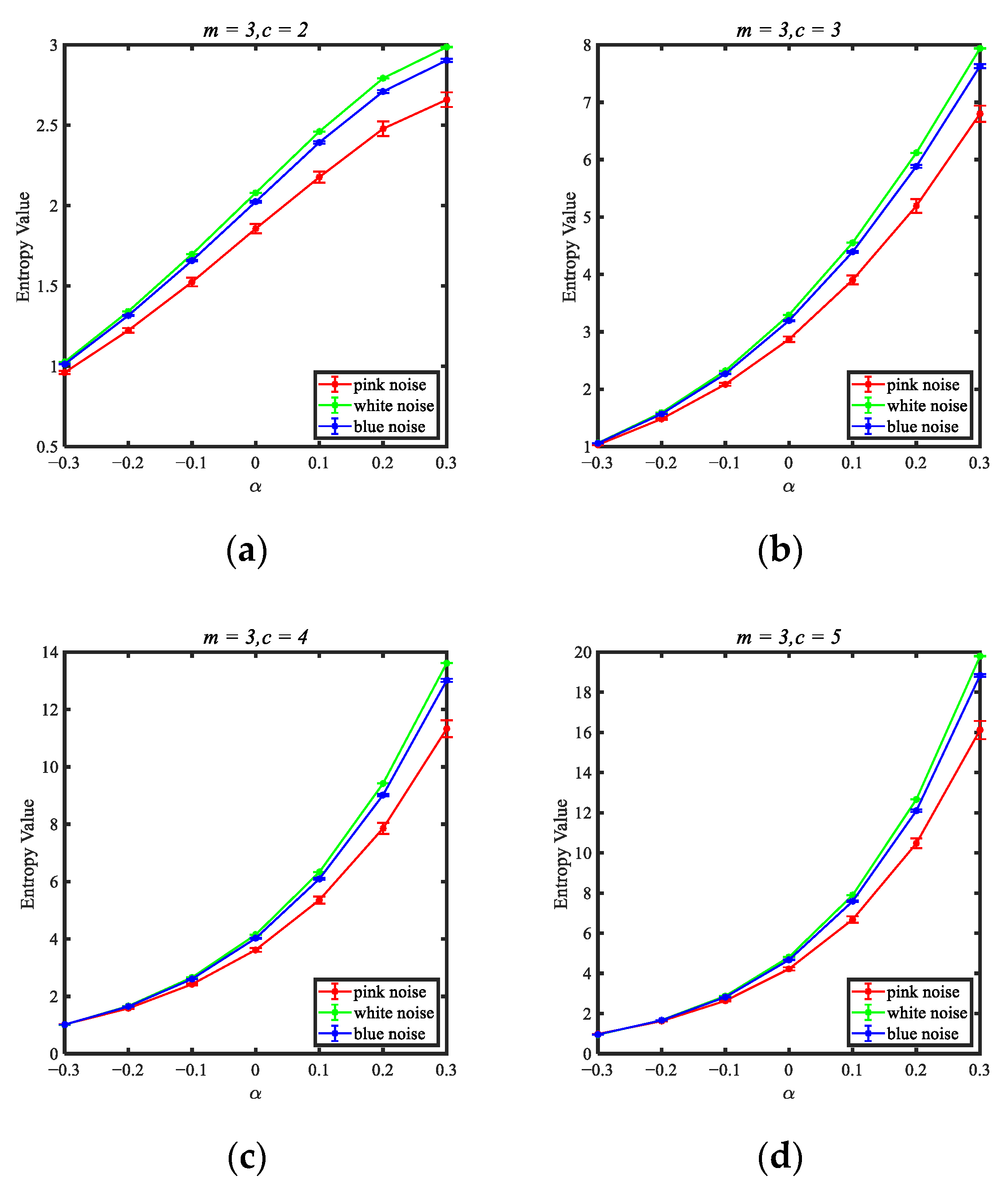
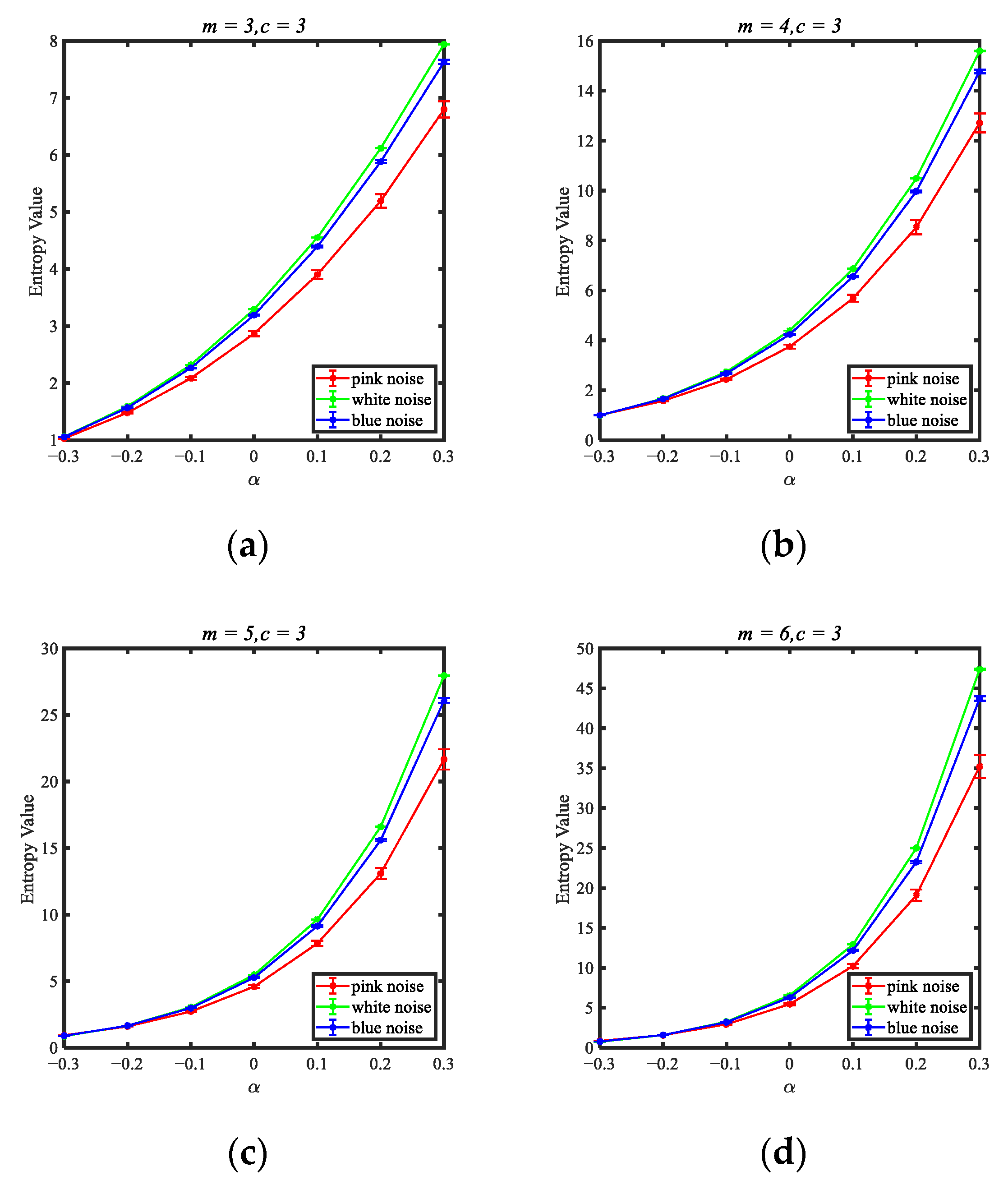
In this subsection, we mainly focus on the discussion of the parameter selection for ${\mathrm{FuzzDE}}_{\alpha }$. For the parameter comparison experiments, 50 separate groups of pink noises, white noises and blue noises are selected [20], each with 2048 sample points. Where white noise consists of a homogeneous mixture of signals of different frequencies, with a variety of frequencies in a haphazard manner. Pink noise enhances the sound intensity of low frequency signals and weakens the intensity of high frequency signals compared to white noise, while blue noise, in contrast, enhances the sound intensity of the high frequency signal on top of the white noise. Using the control variables method, the effects of three ${\mathrm{FuzzDE}}_{\alpha }$ parameters, namely the number of classes $c$, the embedding dimension $m$ and the mapping method, on the mean as well as the standard deviation of the selected noise signals are explored as shown in Figure 2, Figure 3 and Figure 4, respectively.

To begin with, we conduct comparative experiments on the effects of $c$, and the interval is set to an integer between 2 and 5 ($m$ = 3, mapping as NCDF), Figure 2 shows the means and standard deviations of different class number $c$ at different fractional orders.

Comparing the four images, it can be seen that for the average of the entropy values of the three noises, the trend when $m$ equals 3 and $c$ equals 2 is different from the other three in that it has a slope from large to small, while the others are from small to large. However, the general trend is that it increases with the increase of $\alpha$. For the standard deviation of the entropy values of the three noise entropy values, the standard deviation of the pink noise is larger, and the others are smaller, and as $\alpha$ increases, the value of the standard deviation also increases, which is especially evident in the pink noise. In summary, changes in $c$ have an impact on the magnitude of entropy value, but the overall trend in entropy value and the ability to discriminate between different noises does not change as the fractional order changes.

We next discuss the effect of $m$, with the interval set to an integer between 3 and 6 ($c$= 3, mapping as NCDF), Figure 3 is means and standard deviations of different embedding dimensions $m$ at different fractional orders.

Observing the four subplots, for the average of the ${\mathrm{FuzzDE}}_{\alpha }$ values of the three noises, all four cases of taking values show a similar upward trend. For the standard deviation of the entropy values of the three noises, there is only a difference between the exact values and the overall trend is almost the same. Thus, it is clear that the effect of $m$ has a greater impact on the magnitude of the entropy value compared to $c$, but the overall trend and the ability to distinguish between different noises does not change.

Finally, we discuss the effect of the mapping method, which is also an important influencing factor, so we choose different mapping methods for comparison. Figure 4 shows the means and standard deviations of different mapping approaches at different fractional orders, among which the mapping methods include linear mapping (LM), normal cumulative distribution function (NCDF), tangent sigmoid (TANSIG), logarithm sigmoid (LOGSIG), and sorting method (SORT) respectively ($c$ = 3, $m$ = 3) [8,9,10,11].

According to Figure 4, the overall trends of the five mapping methods are very similar, but when using the LM mapping method, the standard deviation of the various noise entropy values is significantly larger, accompanied by the condition that the various noise entropy values overlap each other, which indicates that when the selected mapping method is LM, the stability of ${\mathrm{FuzzDE}}_{\alpha }$ after mapping is relatively weak, and it is difficult to distinguish the three types of noise. While the standard deviation of other mapping methods is relatively small. Therefore, it is concluded that NCDF, LOGISG, TANSIG or SORT are the recommended mapping approaches.

In conclusion, $m$ and $c$ have little effect on the experiment, but a large $m$ is more likely to lead to an increase in ${\mathrm{FuzzDE}}_{\alpha }$ values compared to $c$. Among all mapping methods, only LM is not stable. Therefore, we recommend that $m$ be set to 3–6, $c$ to 2–5 and the mapping method be NCDF, LOGISG, TANSIG or SORT. In the later simulations and the real-world signal experiments, we choose $m$ = 3, $c$ = 4 and the mapping method to be NCDF.

3. Experiments on Simulated Signals

In this section, we focus on demonstrating the usefulness of fractional order calculations on FuzzDE by simulated signals, mainly including noise signals, chirp signal and MIX signal.

3.1. Noise Signals Experiment

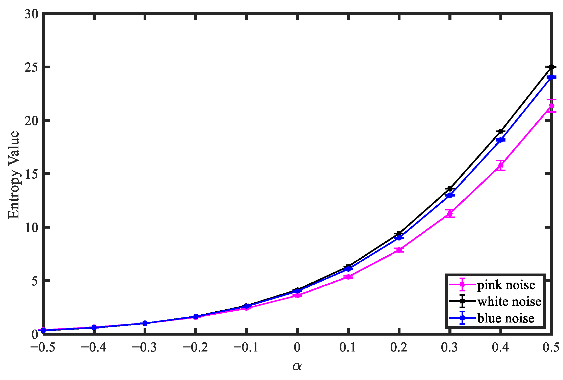
In order to verify the effectiveness of fractional order calculation on FuzzDE, pink noise, white noise and blue noise are selected for comparative experiments, and the fractional orders change from −0.5 to 0.5 with interval 0.1. 100 independent pink noises, white noises and blue noises are created to prove the discrimination ability of fractional order. The means and standard deviations of these 100 ${\mathrm{FuzzDE}}_{\alpha }$. values are calculated respectively as displayed in Figure 5.

As shown in Figure 5, the ${\mathrm{FuzzDE}}_{\alpha }$ value of the three kinds of noise signals has a similar upward trend with the increase of fractional order; when the fractional order is less than −0.1, the mean characteristics of the three noise signals are mixed together; when the fractional order is greater than −0.1, the difference of mean characteristics of the three noise signals gradually increases, and the ${\mathrm{FuzzDE}}_{\alpha }$ value of white noise is the largest, with the smallest standard deviation and the most stable ${\mathrm{FuzzDE}}_{\alpha }$ value. Experiments show that as the fractional order increases (when the fractional order is greater than −0.1), ${\mathrm{FuzzDE}}_{\alpha }$ has a better distinguishing effect on pink noise, white noise and blue noise.

3.2. Chirp Signal Experiment

Chirp signal is a typical unstable signal, and frequency of chirp signal will change over time [22,23]. In order to better show the feature extraction effect of ${\mathrm{FuzzDE}}_{\alpha }$ at different fractional orders, chirp signal is used for simulated experiments. Chirp signal can be expressed as:

$$x\left(t\right)=e^{\left(j2\pi (f_{0}t+\frac{1}{2}k{t}^2)\right)}$$

where $f_0$ is the initiation frequency and is taken as 20 Hz, $k$ is the modulation frequency and is taken as 3, we can understand that the frequency increases from 20 Hz to 80 Hz. The chirp signal lasts 20 s with a sampling frequency of 1000 Hz (20,000 sampling points).

We take the length of the sliding window as 1000 sampling points, and slide backward from the first sampling point with 90% overlap to obtain 190 samples. ${\mathrm{FuzzDE}}_{\alpha }$ for chirp signal of each sample are calculated. Chirp signal (top) and the corresponding different entropy curves (bottom) are shown in Figure 6.

It can be observed from Figure 6 that the waveform of the chirp signal gradually becomes denser as the number of sampling points increases, and the higher the fractional order, the larger the ${\mathrm{FuzzDE}}_{\alpha }$ value as well as the rate of increase of the curve. In a word, the experimental results show that the higher the fractional order of ${\mathrm{FuzzDE}}_{\alpha }$, the better performance of ${\mathrm{FuzzDE}}_{\alpha }$ in chirp signal feature extraction.

3.3. MIX Signal Experiment

In order to study the influence for fractional order of ${\mathrm{FuzzDE}}_{\alpha }$ on the effect of feature extraction, we select MIX signal for simulated experiments. MIX signal describes a stochastic sequence that progressively turns into a periodic time series [24,25], which can be expressed as:

$$\{\begin{array}{c}MIX\left(t\right)=\left(1-Z\right)\times X\left(t\right)+Z\times Y\left(t\right)\\ X\left(t\right)=\sqrt{2}sin\frac{2\pi t}{12}\end{array}$$

where $X\left(t\right)$ is a periodic signal, the value of $Y\left(t\right)$ is uniformly distributed from $-\sqrt{3}$ to $\sqrt{3}$, and Z is a random number taking 1 or 0 with probabilities P and 1 − P, respectively, and decreasing linearly from 0.99 at the beginning to 0.01 at the end. The sampling frequency of mix signal is 1000 Hz, with a total of 20 s. We take the length of sliding window as 1000 sampling points, and slide backward from the first sampling point with 90% overlap to obtain 190 samples. MIX signal (top) and the corresponding different entropy curves (bottom) are shown in Figure 7.

As can be seen from Figure 7, the MIX signal changes from dense to sparse as the number of sampling points increases; the value of ${\mathrm{FuzzDE}}_{\alpha }$ decreases as the number of sampling points increases; the higher the fractional order, the larger the ${\mathrm{FuzzDE}}_{\alpha }$ value and the rate of decline of the curve also increases. Therefore, we can conclude that an increase in fractional order can better reflect the complexity of the MIX signal.

4. Experiments on Bearing Fault Diagnosis

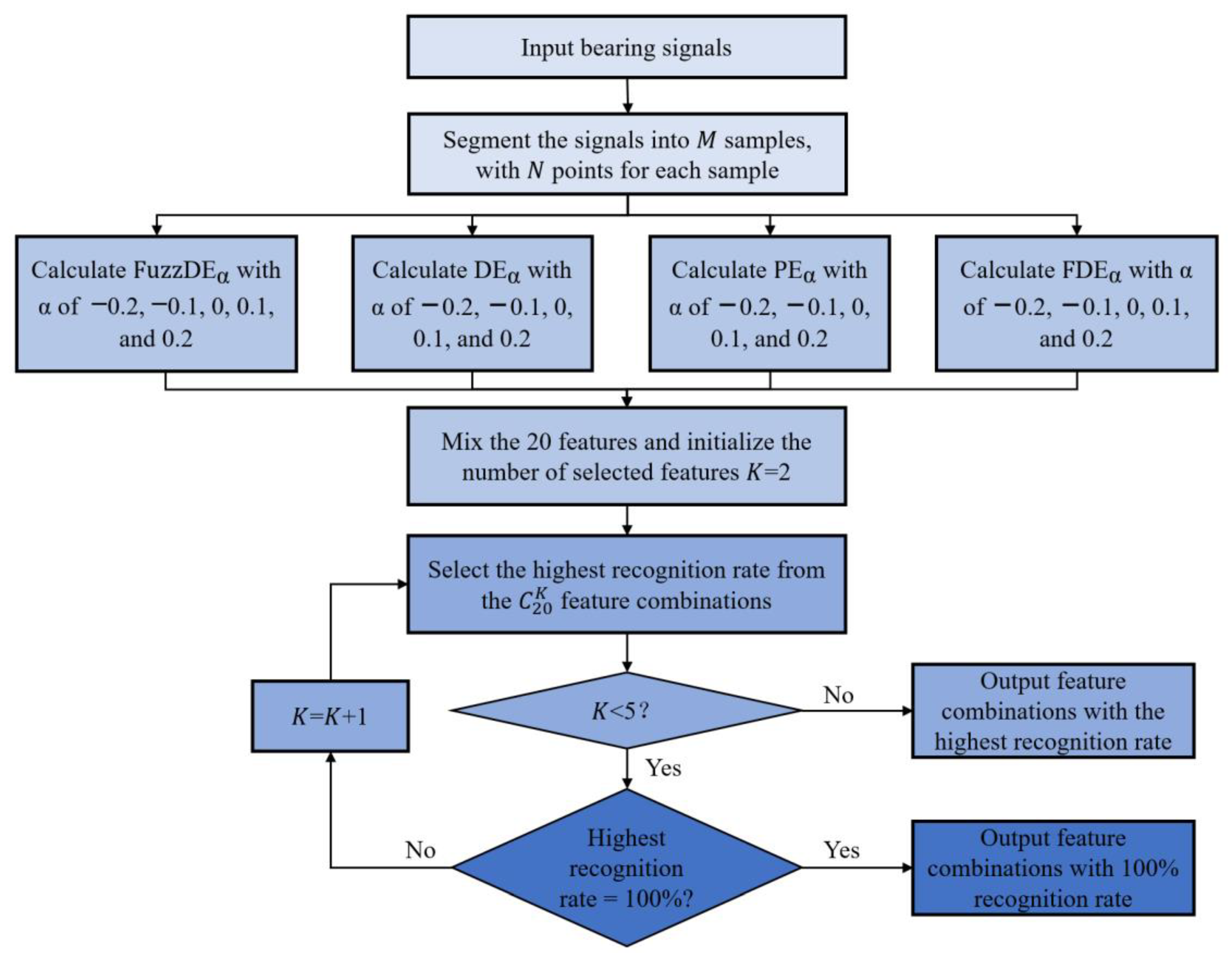
In this section, we focus on the bearing fault diagnosis, and achieve early prevention in order to avoid economic losses and even personal safety due to different bearing faults. Since entropy can be used to detect changes in the dynamics of weak time series, the higher the entropy value, the more unstable the time series and vice versa. At the same fault size, different faults have similar amplitude-frequency features, but their bearing fault complexity and dynamics changes are different, and these changes can be reflected in successive subsequences, for which entropy features can be extracted for fault diagnosis of the bearing signals. The experiments in this section are mainly to verify the effectiveness of ${\mathrm{FuzzDE}}_{\alpha }$ for bearing fault diagnosis, and the proposed mixed features bearing fault diagnosis method experimental flow chart is shown in Figure 8, with the following steps:

Step 1: Input the real-world bearing signals of ten different classes.

Step 2: Segment the input signals into $M$ samples, each with $N$ sample points, by which way, we receive a total of $M$ samples for each class of signal.

Step 3: For each sample, calculate their ${\mathrm{FuzzDE}}_{\alpha }$ values at different fractional orders. For the purpose of contrast, we also introduce fractional order DE (${\mathrm{DE}}_{\alpha }$), fractional order PE (${\mathrm{PE}}_{\alpha }$) and fractional order FDE (${\mathrm{FDE}}_{\alpha }$) for comparison, with fractional orders of −0.2, −0.1, 0, 0.1, and 0.2 respectively.

Step 4: Mix the 20 features obtained in Step 3 and set the number of selected features to $K$ (initialized to 2), by which way we can acquire a total of $C_{20}^K$ combinations.

Step 5: Calculate the recognition rate of all $C_{20}^K$ combinations and select the combination with the highest recognition rate.

Step 6: Determine the direction of the process by the number of features selected, and if $K$ < 5, skip to Step 7; otherwise, output the combination of 5 features with the highest recognition rate and the corresponding recognition rate, as a way to avoid the increased computational consumption when the recognition rate has reached the threshold.

Step 7: Determine the direction of the process by the highest recognition rate among $K$ feature combinations. If the recognition rate reaches 100%, then output these feature combinations; otherwise, let $K$ = $K$ + 1 and back to Step 5.

4.1. Analysis of Experiment Data

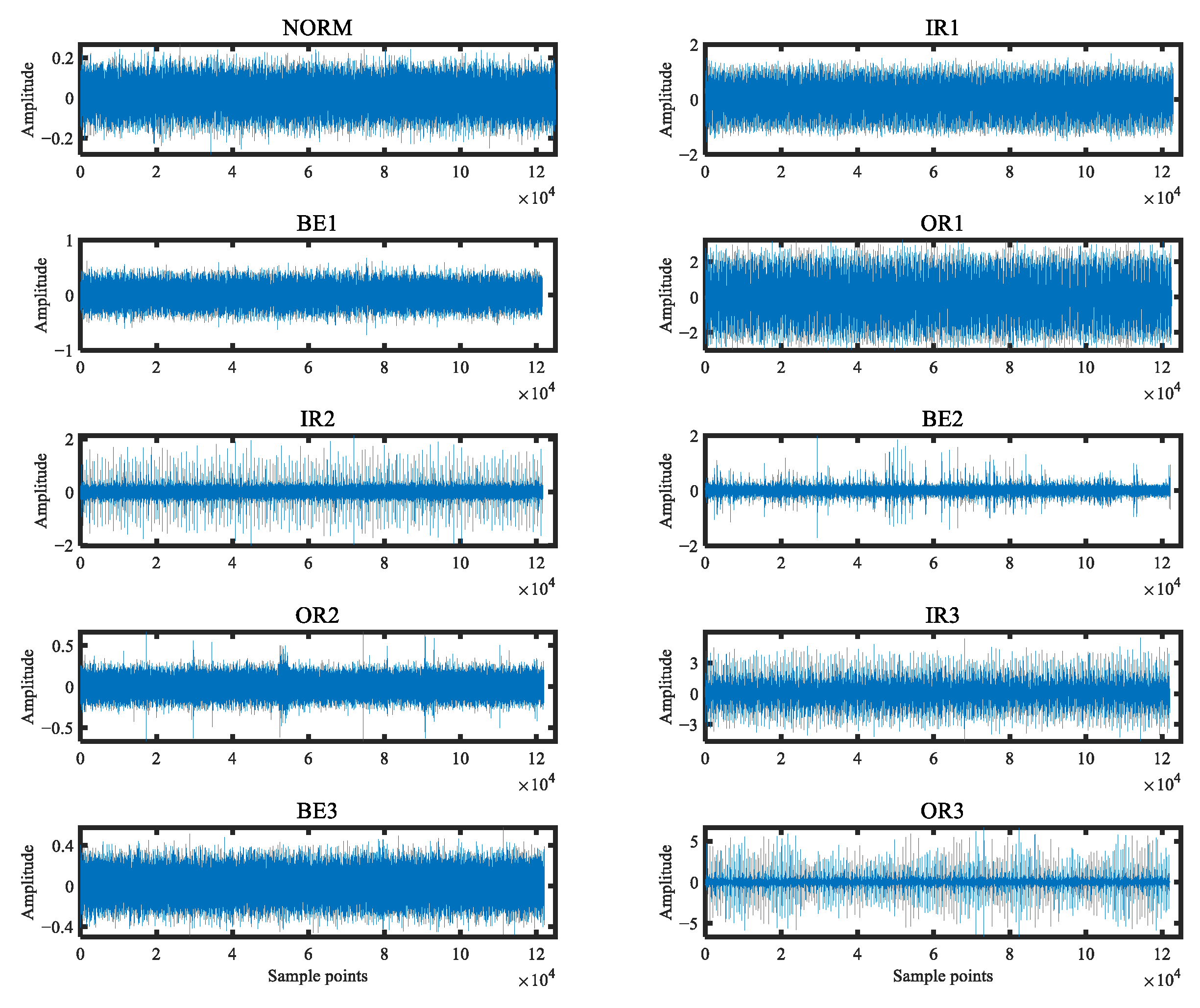
This section employs the bearing signal obtained from Case Western Reserve University (CWRU) [26] to verify the effectiveness of the proposed ${\mathrm{FuzzDE}}_{\alpha }$. The bearing under test is a deep groove ball bearing type SKF6205 (CWRU, Cleveland, America) with a motor speed set to 1730 r/min and a load of 3 hp. The original bearing signal is acquired by collecting the acceleration sensor installed at the driving end, and the sampling frequency is 12 kHz. Depending on the states of the bearing and the diameters of the failure, there are 10 different types of bearing signals marked NORM, IR1, BE1, OR1, IR2, BE2, OR2, IR3, BE3 and OR3, all damage is caused by electro discharge machining as a single point of damage. The details of the selected bearing signals are shown in

Table 1. Details of the selected bearing signals.

Class	Label	Fault Size (mm)	Selected Data
Normal	NORM	0	100_normal_3
Inner race fault	IR1	0.1778	108_IR007_3
Balling element fault	BE1	0.1778	121_B007_3
Outer race fault	OR1	0.1778	133_OR007@6_3
Inner race fault	IR2	0.3556	172_IR014_3
Balling element fault	BE2	0.3556	188_B014_3
Outer race fault	OR2	0.3556	200_OR014@6_3
Inner race fault	IR3	0.5334	212_IR021_3
Balling element fault	BE3	0.5334	225_B021_3
Outer race fault	OR3	0.5334	237_OR021@6_3

. For each class of bearing signal, the length of sample points is 120,000, and Figure 9 shows the time domain distribution of ten classes of bearing signals.

4.2. Single Feature Extraction and Classification

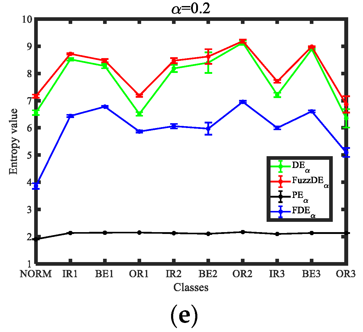
The ten classes of bearing signals are used as the object of the experiment for single feature extraction. There are 50 samples for each type of bearing signal, and each sample contains 2048 sample points. While calculating the ${\mathrm{FuzzDE}}_{\alpha }$ of the bearing signal, the ${\mathrm{DE}}_{\alpha }$, ${\mathrm{PE}}_{\alpha }$, and ${\mathrm{FDE}}_{\alpha }$ are calculated respectively as comparative analysis. The parameter settings are as follows: embedding dimension m is 3, class number c is 4, and the range of fractal order $\mathsf{\alpha }$ is from −0.2 to 0.2 with interval 0.1. For other fractional entropies, the parameter settings are the same as ${\mathrm{FuzzDE}}_{\alpha }$. The Distribution of fractional entropy features of different classes of bearing signals are exhibited in Figure 10.

From Figure 10, for the four types of fractional entropies, it is difficult to completely distinguish all ten types of bearing signals under different fractional order; for ${\mathrm{FuzzDE}}_{\alpha }$, ${\mathrm{DE}}_{\alpha ,}$, and ${\mathrm{FDE}}_{\alpha }$, there is always some standard deviation of fractional entropy values close to each other for bearing signals; in addition, the standard deviation of fractional entropy values are significantly higher than that of ${\mathrm{PE}}_{\alpha }$ under different fractional order, for ${\mathrm{PE}}_{\alpha }$, the standard deviations of fractional entropy values for ten classes of bearing signals are all very close, which is difficult to distinguish. Furthermore, we employ KNN to classify the ten classes of bearing signals, in which there are 50 samples for each type of bearing signal, the first 25 samples are training samples, and the rest samples are test samples.

Table 2. Classification recognition rate of different entropies at various fractional orders.

Entropy	Recognition Rates (%)
	$\mathbf{\alpha }=-0.2$	$\mathbf{\alpha }=-0.1$	$\mathbf{\alpha }=0$	$\mathbf{\alpha }=0.1$	$\mathbf{\alpha }=0.2$
${\mathrm{FuzzDE}}_{\alpha }$	82.8	81.6	74	68.4	67.6
${\mathrm{DE}}_{\alpha }$	76.4	79.6	76.4	71.2	66.0
${\mathrm{PE}}_{\alpha }$	59.6	56.8	58.4	56.8	54.0
${\mathrm{FDE}}_{\alpha }$	79.2	82.8	78.4	77.6	80.4

illustrates the classification recognition rate of different entropies at various fractional orders.

It can be seen from Table 2, for four classes of fractional entropies, the recognition rates of bearing signals are all lower than 85% under different fractional orders, and the recognition effect is poor. Therefore, it is difficult to distinguish ten classes of signals with one feature.

4.3. Double Features Extraction and Classification

In order to improve recognition performance and demonstrate the effectiveness of the mixed feature extraction method proposed in this paper, we choose different entropy-based feature extraction methods, extract any two fractional orders with the same entropy and choose the best combinations of fractional orders. Since fractional order $\alpha$ has 5 values, a total of ${\mathrm{C}}_5^2$ combinations can be obtained by each entropy-based feature extraction method. In addition, we use the mixed feature extraction method proposed in this paper to calculate the highest recognition rate, with a total of ${\mathrm{C}}_{20}^2$ combinations.

Table 3. Highest classification recognition rates for each feature extraction method (double features).

Feature Extraction Methods	Combinations	Recognition Rate (%)
${\mathrm{FuzzDE}}_{\alpha }$-based	${\mathrm{FuzzDE}}_{\alpha =0} \&{ \mathrm{FuzzDE}}_{\alpha =0.2}$	91.6
${\mathrm{DE}}_{\alpha }$-based	${\mathrm{DE}}_{\alpha =0} \&{ \mathrm{DE}}_{\alpha =0.2}$	88.4
${\mathrm{PE}}_{\alpha }$-based	${\mathrm{PE}}_{\alpha =-0.2} \&{ \mathrm{PE}}_{\alpha =0.1}$	58.4
${\mathrm{FDE}}_{\alpha }$-based	${\mathrm{FDE}}_{\alpha =-0.1} \&{ \mathrm{FDE}}_{\alpha =0}$	90.0
Proposed method	${\mathrm{FuzzDE}}_{\alpha =0.1}$& ${\mathrm{FDE}}_{\alpha =0.1}$ (1 of 3)	99.6

demonstrate the highest classification recognition rates for each feature extraction method when double features are selected.

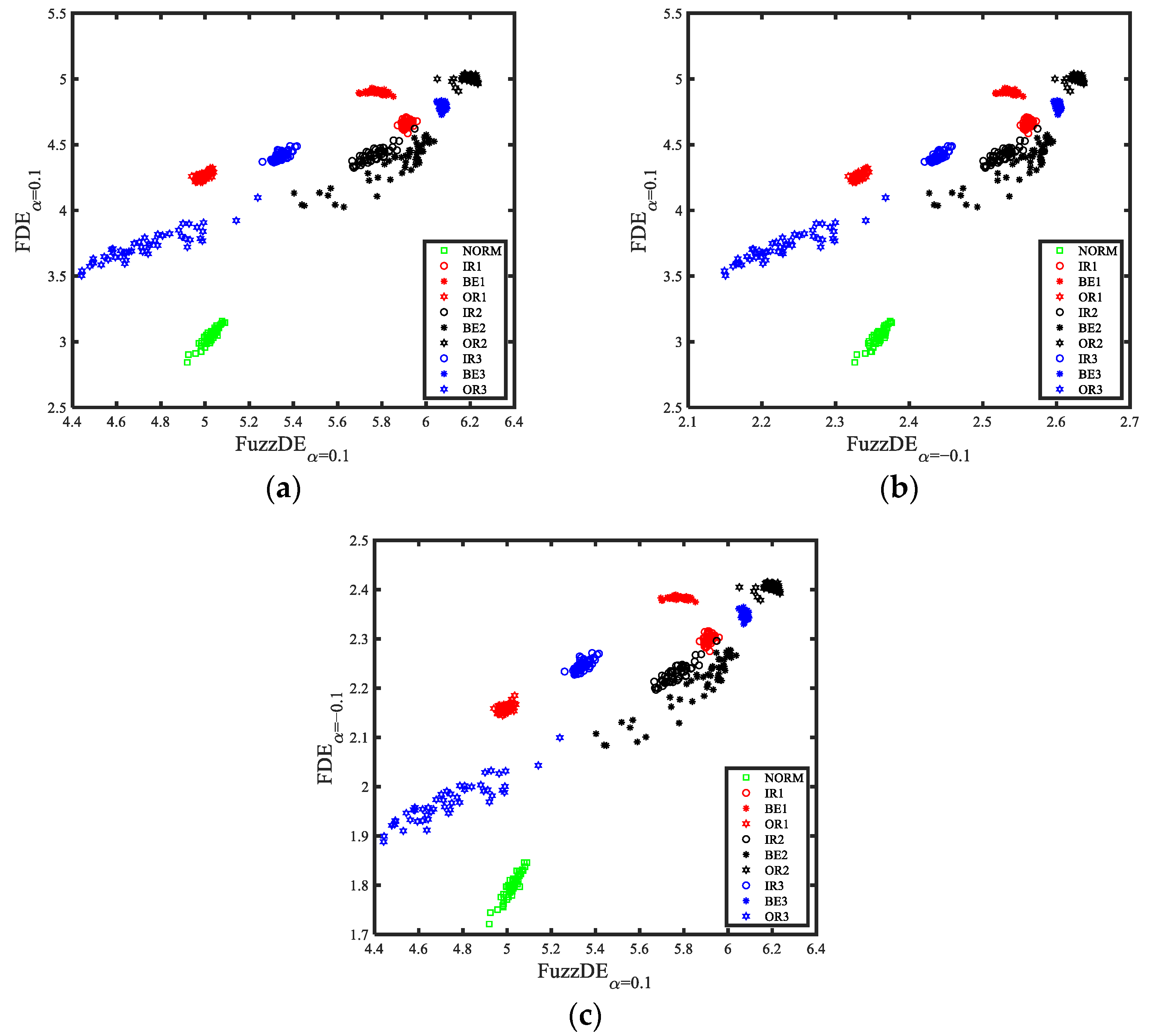
In Table 3, ${\mathrm{FuzzDE}}_{\alpha =0}$ & ${\mathrm{FuzzDE}}_{\alpha =0.2}$ represents ${\mathrm{FuzzDE}}_{\alpha }$ when fractional order $\alpha$is 0 and 0.2 respectively, other combinations of entropy are the same for ${\mathrm{FuzzDE}}_{\alpha =0}$ & ${\mathrm{FuzzDE}}_{\alpha =0.2}$. As can be observed in Table 3, ${\mathrm{FuzzDE}}_{\alpha }$-based feature extraction method has the best classification effect among the four entropy-based feature extraction methods, but the highest recognition rate is only 91.6%, which cannot fully recognize the bearing signals. Nevertheless, the mixed feature extraction method proposed in this paper can reach a maximum classification rate of 99.6%, significantly higher than the 91.6% of ${\mathrm{FuzzDE}}_{\alpha }$-based feature extraction method, and there are three combinations in total, namely ${\mathrm{FuzzDE}}_{\alpha =0.1}$ & ${\mathrm{FDE}}_{\alpha =0.1}$, ${\mathrm{FuzzDE}}_{\alpha =-0.1}$ & ${\mathrm{FDE}}_{\alpha =0.1}$ and ${\mathrm{FuzzDE}}_{\alpha =0.1}$ & ${\mathrm{FDE}}_{\alpha =-0.1}$. It is noteworthy that when reaching the highest recognition rate, the three combinations all contain ${\mathrm{FuzzDE}}_{\alpha }$, which further proves the importance of ${\mathrm{FuzzDE}}_{\alpha }$ in bearing fault diagnosis recognition. Figure 11 shows the distribution of the highest classification recognition rate of mixed double features.

As can be seen from Figure 11, under the mixed double features, the distribution of each type of bearing signal is relatively concentrated, and the overlapping part is very small. However, there are few samples that are not completely distinguishable, for example, a small percentage of IR1 and IR2 samples are mixed. In summary, compared with the entropy-based feature extraction methods, the mixed feature extraction method proposed in this paper further improves the recognition rate and can better distinguish the ten classes of bearing signals. To sum up, mixed double features extraction method can well distinguish the ten classes of bearing signals.

4.4. Triple Features Extraction and Classification

In order to further improve the recognition rate of bearing fault diagnosis, we set the number of selected features H to 3. The rest of the steps are the same as Section 4.3, and

Table 4. Highest classification recognition rates for each feature extraction method (triple features).

Feature Extraction Methods	Combinations	Recognition Rate (%)
${\mathrm{FuzzDE}}_{\alpha }$-based	${\mathrm{FuzzDE}}_{\alpha =-0.1} \&{ \mathrm{FuzzDE}}_{\alpha =0} \&{ \mathrm{FuzzDE}}_{\alpha =0.2}$	92
${\mathrm{DE}}_{\alpha }$-based	${\mathrm{DE}}_{\alpha =-0.1} \&{ \mathrm{DE}}_{\alpha =0} \&{ \mathrm{DE}}_{\alpha =0.2}$	92
${\mathrm{PE}}_{\alpha }$-based	${\mathrm{PE}}_{\alpha =-0.2} \&{ \mathrm{PE}}_{\alpha =0} \&{ \mathrm{PE}}_{\alpha =0.1}$	58
${\mathrm{FDE}}_{\alpha }$-based	${\mathrm{FDE}}_{\alpha =-0.2} \&{ \mathrm{FDE}}_{\alpha =-0.1} \&{ \mathrm{FDE}}_{\alpha =0}$	91.6
Proposed method	${\mathrm{FuzzDE}}_{\alpha =-0.1} \&{ \mathrm{PE}}_{\alpha =-0.2} \&{ \mathrm{FuzzDE}}_{\alpha =0.1}$ (1 of 15)	100

shows the highest classification recognition rates for each feature extraction method when triple features are selected.

From Table 4, it can be seen that as the number of features increases, the recognition rates of the feature extraction methods based on ${\mathrm{FuzzDE}}_{\alpha }$, ${\mathrm{DE}}_{\alpha }$ and ${\mathrm{FDE}}_{\alpha }$ all improved, but the fault diagnosis performance is still much less than that of the mixed double features in Table 3, which indicates that different fractional order features with the same entropy still have certain limitations. Furthermore, we can also observe from Table 4 that the mixed feature extraction method proposed in this paper achieves a recognition rate of 100% for 15 combinations when triple features are selected, further demonstrating the excellent performance of the mixed feature extraction method for bearing fault diagnosis. To visualize the specific details of these 15 combinations,

Table 5. Number of occurrences of each feature in the combination of the mixed triple features with 100% recognition rate.

Feature	Appear Times
${\mathrm{FuzzDE}}_{\alpha =-0.1}$	$11$
${\mathrm{FuzzDE}}_{\alpha =-0.2}$	$4$
${\mathrm{PE}}_{\alpha =-0.2}$	$2$
${\mathrm{PE}}_{\alpha =-0.1}$	$3$
${\mathrm{PE}}_{\alpha =0}$	$3$
${\mathrm{PE}}_{\alpha =0.1}$	$4$
${\mathrm{PE}}_{\alpha =0.2}$	$3$
${\mathrm{FDE}}_{\alpha =-0.1}$	$6$
${\mathrm{FDE}}_{\alpha =0}$	$5$
${\mathrm{FDE}}_{\alpha =0.1}$	$4$

shows the number of occurrences of each feature in the combinations with 100% recognition rate.

It is clear from Table 5 that ${\mathrm{FuzzDE}}_{\alpha =-0.1}$ has the highest number of occurrences at 11, far more than any other features, which proves the efficiency of ${\mathrm{FuzzDE}}_{\alpha }$ in bearing fault diagnosis. In addition, among the feature combinations with 100% recognition rate, only ${\mathrm{DE}}_{\alpha }$ is absent, which is due to the fact that $\mathrm{FuzzDE}$ is an improvement on DE, further validating the conclusion that $\mathrm{FuzzDE}$ is more differentiable than DE. We can also find that although the ${\mathrm{PE}}_{\alpha }$ has a low recognition rate on bearing fault diagnosis, it can accurately classify some samples that cannot be correctly classified by other entropies. Hence, we can also conclude that different entropies can distinguish different signal classes, and following the mixed feature extraction method proposed in this paper, while selecting mixed fractional order entropies simultaneously can effectively improve the performance of bearing fault diagnosis.

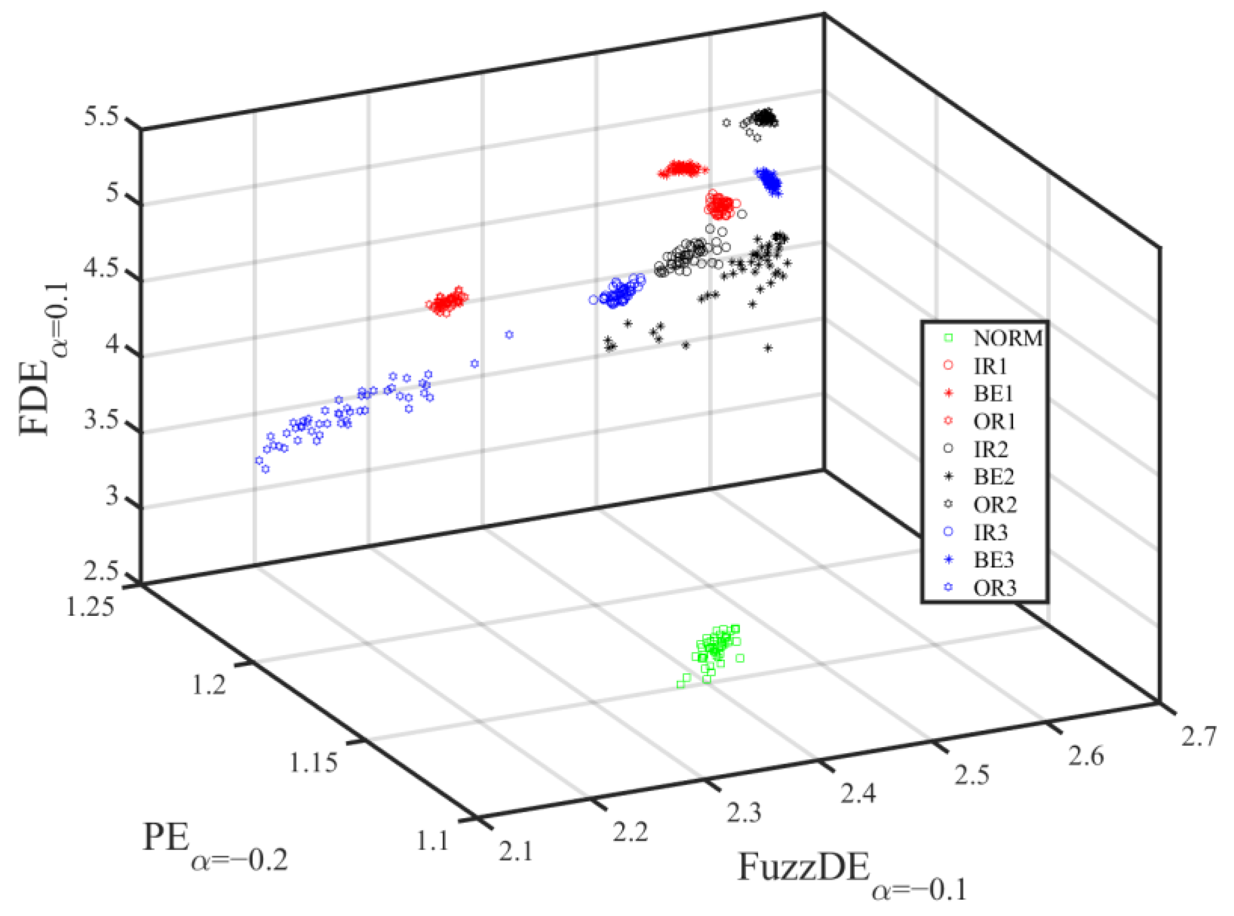
Figure 12 depicts the distribution of the triple features at 100% recognition rate with the combination of ${\mathrm{FuzzDE}}_{\alpha =-0.1}$, ${\mathrm{PE}}_{\alpha =-0.2}$ and ${\mathrm{FDE}}_{\alpha =0.1}$. Compared to Figure 11, we can intuitively find that Figure 12 can perfectly distinguish between IR1 as well as IR2, which are two different sizes of the same fault class, and it is obvious that the mixed double features distribution cannot achieve such results.

5. Conclusions

In this paper, a new non-linear dynamic parameter is proposed, and a mixed features extraction method is put forward based on this new parameter. The main conclusions are as follows.

• Fractional order calculation is introduced on the basis of fuzzy dispersion entropy (FuzzDE), and a new entropy called fractional order FDE (${\mathrm{FuzzDE}}_{\alpha }$) is proposed. Simulated experiments have shown that compared with $\mathrm{FuzzDE}$, ${\mathrm{FuzzDE}}_{\alpha }$ can provide more features of greater sensitivity to changes in the dynamics of the time series.
• ${\mathrm{FuzzDE}}_{\alpha }$ is combined with ${\mathrm{DE}}_{\alpha }$, ${\mathrm{PE}}_{\alpha }$ as well as ${\mathrm{FDE}}_{\alpha }$ to present a mixed features extraction method. For ten classes of bearing signals, the proposed mixed features fault diagnosis method achieves 100% recognition rate at only triple features.
• Regardless of how many features are selected, the ${\mathrm{FuzzDE}}_{\alpha }$ proposed in this paper is the most effective in fault diagnosis compared to the other three fractional order entropies, where ${\mathrm{FuzzDE}}_{\alpha =-0.1}$ appears a total of 11 times in the combination of the triple features with the recognition rate of 100%

References

1. Berger, A.L.; Della Pietra, V.J.; Della Pietra, S.A. A maximum entropy approach to natural language processing. Comput. Linguist. 1996, 22, 39–71. [Google Scholar]
2. Martyushev, L.M.; Seleznevb, V.D. Maximum entropy production principle in physics, chemistry and biology. Phys. Rep. 2006, 426, 1–45. [Google Scholar] [CrossRef]
3. Rostaghi, M.; Khatibi, M.M.; Ashory, M.R.; Azami, H. Bearing Fault Diagnosis Using Refined Composite Generalized Multiscale Dispersion Entropy-Based Skewness and Variance and Multiclass FCM-ANFIS. Entropy 2021, 23, 1510. [Google Scholar] [CrossRef] [PubMed]
4. Zhang, X.; Liang, Y.; Zhou, J.; Zang, Y. A novel bearing fault diagnosis model integrated permutation entropy, ensemble empirical mode decomposition and optimized SVM. Measurement 2015, 69, 164–179. [Google Scholar] [CrossRef]
5. Yan, R.; Liu, Y.; Gao, R. Permutation entropy: A nonlinear statistical measure for status characterization of rotary machines. Mech. Syst. Signal Process. 2012, 29, 474–484. [Google Scholar] [CrossRef]
6. Zhang, X.; Wang, H.; Ren, M.; He, M.; Jin, L. Rolling Bearing Fault Diagnosis Based on Multiscale Permutation Entropy and SOA-SVM. Machines 2022, 10, 485. [Google Scholar] [CrossRef]
7. Ying, W.; Tong, J.; Dong, Z.; Pan, H.; Liu, Q.; Zheng, J. Composite Multivariate Multi-Scale Permutation Entropy and Laplacian Score Based Fault Diagnosis of Rolling Bearing. Entropy 2022, 24, 160. [Google Scholar] [CrossRef]
8. Rostaghi, M.; Azami, H. Dispersion Entropy: A Measure for Time Series Analysis. IEEE Signal Process. Lett. 2016, 23, 610–614. [Google Scholar] [CrossRef]
9. Gu, C.; Qiao, X.; Li, H. Misfire Fault Diagnosis Method for Diesel Engine Based on MEMD and Dispersion Entropy. Shock Vib. 2021, 5, 1–14. [Google Scholar] [CrossRef]
10. Azami, H.; Fernandez, A.; Escudero, J. Multivariate Multiscale Dispersion Entropy of Biomedical Times Series. Entropy 2017, 21, 913. [Google Scholar] [CrossRef]
11. Azami, H.; Escudero, J. Amplitude- and Fluctuation-Based Dispersion Entropy. Entropy 2018, 20, 210. [Google Scholar] [CrossRef] [PubMed] [Green Version]
12. Li, Y.; Gao, X.; Wang, L. Reverse Dispersion Entropy: A New Complexity Measure for Sensor Signal. Sensors 2019, 19, 5203. [Google Scholar] [CrossRef] [PubMed]
13. Li, Y.; Jiao, S.; Gao, X. A novel signal feature extraction technology based on empirical wavelet transform and reverse dispersion entropy. Def. Technol. 2021, 17, 1625–1635. [Google Scholar] [CrossRef]
14. Jiao, S.; Geng, B.; Li, Y. Fluctuation-based reverse dispersion entropy and its applications to signal classification. Appl. Acoust. 2021, 175, 107857. [Google Scholar] [CrossRef]
15. Rostaghi, M.; Khatibi, M.M.; Ashory, M.R.; Azami, H. Fuzzy Dispersion Entropy: A Nonlinear Measure for Signal Analysis. IEEE Trans. Fuzzy Syst. 2022, 30, 3785–3796. [Google Scholar] [CrossRef]
16. Ali, K. Fractional order entropy: New perspectives. Opt.-Int. J. Light Electron Opt. 2016, 127, 9172–9177. [Google Scholar]
17. Ingo, C.; Magin, R.L.; Parrish, T.B. New Insights into the Fractional Order Diffusion Equation Using Entropy and Kurtosis. Entropy 2014, 16, 5838–5852. [Google Scholar] [CrossRef] [PubMed]
18. Zunino, L.; Pérez, D.G.; Martín, M.T. Permutation entropy of fractional Brownian motion and fractional Gaussian noise. Phys. Lett. A 2008, 372, 4768–4774. [Google Scholar] [CrossRef]
19. He, S.; Sun, K. Fractional fuzzy entropy algorithm and the complexity analysis for nonlinear time series. Eur. Phys. J. Spec. Top. 2018, 227, 943–957. [Google Scholar] [CrossRef]
20. Zheng, J.; Pan, H. Use of generalized refined composite multiscale fractional dispersion entropy to diagnose the faults of rolling bearing. Nonlinear Dyn. 2021, 101, 1417–1440. [Google Scholar] [CrossRef]
21. Li, Y.; Mu, L. Particle Swarm Optimization Fractional Slope Entropy: A New Time Series Complexity Indicator for Bearing Fault Diagnosis. Fractal Fract. 2022, 6, 345. [Google Scholar] [CrossRef]
22. Azami, H.; Escudero, J. Improved multiscale permutation entropy for biomedical signal analysis: Interpretation and application to electroencephalogram recordings. Biomed. Signal Process. Control 2016, 23, 28–41. [Google Scholar] [CrossRef] [Green Version]
23. Azami, H.; Fernandez, A.; Escudero, J. Refined Multiscale Fuzzy Entropy based on Standard Deviation for Biomedical Signal Analysis. Med. Biol. Eng. Comput. 2017, 55, 2037–2052. [Google Scholar] [CrossRef] [PubMed]
24. Wu, G.; Baleanu, D. Chaos synchronization of the discrete fractional logistic map. Signal Process. 2014, 102, 96–99. [Google Scholar] [CrossRef]
25. Li, Y.; Liu, F.; Wang, S. Multi-scale Symbolic Lempel-Ziv: An Effective Feature Extraction Approach for Fault Diagnosis of Railway Vehicle Systems. IEEE Trans. Ind. Inform. 2021, 17, 199–208. [Google Scholar] [CrossRef]
26. Case Western Reserve University. Available online: http://csegroups.case.edu/bearingdatacenter/pages/download-data-file (accessed on 1 July 2022).
Figure 1. Fuzzy membership function.
Fractalfract 06 00544 g001
Figure 2. Means and standard deviations of different class number c at different fractional orders. (a) c = 2; (b) c = 3; (c) c = 4; (d)   c = 5.
Fractalfract 06 00544 g002
Figure 3. Means and standard deviations of different embedding dimensions m at different fractional orders. (a) m = 3; (b) m = 4; (c) m = 5; (d)   m = 6.
Fractalfract 06 00544 g003
Figure 4. Means and standard deviations of different mapping approaches at different fractional orders. (a) LM; (b) NCDF; (c) LOGISG; (d) TANSIG; (e) SORT.
Fractalfract 06 00544 g004
Figure 5. Means and standard deviations of different fractional order entropies under noise signals.
Fractalfract 06 00544 g005
Figure 6. Chirp signal (top) and the corresponding different entropy curves (bottom).
Fractalfract 06 00544 g006
Figure 7. MIX signal (top) and the corresponding different entropy curves (bottom).
Fractalfract 06 00544 g007
Figure 8. Flow chart of the proposed mixed features bearing fault diagnosis method.
Fractalfract 06 00544 g008
Figure 9. Time domain distribution of ten classes of bearing signals.
Fractalfract 06 00544 g009
Figure 10. Distribution of fractional entropy features of different classes of bearing signals. (a) α = −0.2; (b)   α = −0.1; (c)   α = 0; (d)   α = 0.1; (e)   α = 0.2.
Fractalfract 06 00544 g010aFractalfract 06 00544 g010b
Figure 11. Distribution of the highest classification recognition rate of mixed double features. (a) FuzzDE α = 0 . 1 . & FDE α = 0 . 1 ; (b)   FuzzDE α = - 0 . 1 & FDE α = 0 . 1 ; (c) FuzzDE α = 0 . 1 & FDE α = - 0 . 1 .
Fractalfract 06 00544 g011
Figure 12. Distribution of the mixed triple features at 100% recognition rate ( FuzzDE α = - 0 . 1 , PE α = - 0 . 2 , FDE α = 0 . 1 ).
Fractalfract 06 00544 g012