Article

Scaling Region of Weierstrass-Mandelbrot Function: Improvement Strategies for Fractal Ideality and Signal Simulation

1
Division of Advanced Manufacturing, Shenzhen International Graduate School, Tsinghua University, Shenzhen 518055, China
2
Tsinghua-Berkeley Shenzhen Institute, Tsinghua University, Shenzhen 518055, China
3
Department of Mechanical Engineering, Tsinghua University, Beijing 100084, China
*
Authors to whom correspondence should be addressed.
Fractal Fract. 2022, 6(10), 542; https://doi.org/10.3390/fractalfract6100542
Submission received: 31 July 2022 / Revised: 14 September 2022 / Accepted: 20 September 2022 / Published: 26 September 2022

Abstract

:
Fractal dimension (D) is widely utilized in various fields to quantify the complexity of signals and other features. However, the fractal nature is limited to a certain scope of concerned scales, i.e., scaling region, even for a theoretically fractal profile generated through the Weierstrass-Mandelbrot (W-M) function. In this study, the scaling characteristics curves of profiles were calculated by using the roughness scaling extraction (RSE) algorithm, and an interception method was proposed to locate the two ends of the scaling region, which were named corner and drop phenomena, respectively. The results indicated that two factors, sampling length and flattening order, in the RSE algorithm could influence the scaling region length significantly. Based on the scaling region interception method and the above findings, the RSE algorithm was optimized to improve the accuracy of the D calculation, and the influence of sampling length was discussed by comparing the lower critical condition of the W-M function. To improve the ideality of fractal curves generated through the W-M function, the strategy of reducing the fundamental frequency was proposed to enlarge the scaling region. Moreover, the strategy of opposite operation was also proposed to improve the consistency of generated curves with actual signals, which could be conducive to practical simulations.

1. Introduction

Fractal theory has been established to interpret the characteristics of self-similar or self-affine features [1,2,3]. For such features, when the measurement scale (L) is lowered, finer structures can be observed. In order to quantify the complexity of fractal objects, the concept of fractal dimension (D) was proposed by Mandelbrot [4] and widely used [5,6]. In the field of mathematics, there are strictly self-similar Cantor discrete point sets, Koch curve sets and so on. In the research on natural objects, it is also believed that fractal geometry could be applied, such as machining signals [7,8,9], micro-structure of new materials [10,11,12], surfaces topography [13,14,15], etc.
However, not all objects have perfect fractal characteristics [16,17]. Once they exceed a certain range, they will show non-fractal characteristics. In the region that has fractal characteristics, the root-mean-squared roughness ( R q , also known as RMS) usually shows scaling characteristics, which is called the scaling region. D is then calculated using the scaling region. In order to accurately calculate the value of D, the scaling region needs to be extracted. Yokoya et al. [18] proposed an empirical formula to calculate the upper and lower limits of the scaling region, but due to the lack of objective standards, this method had poor general applicability. In addition, other fitting methods, including three-line segment fitting [19], curve-line-curve fitting [20] and S-shaped curve fitting [21], were used to extract the scaling region. Due to the error between the fitted curve and the actual R q -L curve, the calculation result of D was inaccurate. Chen et al. [22] used the K-means method to intercept the scaling region, while the clustering algorithm might lead to the local optimal solution. Zhou et al. [23] proposed a density peak clustering algorithm based on machine learning to identify the scaling region, which was relatively complex and difficult to implement.
There are many algorithms for calculating the D value, and the Weierstrass-Mandelbrot (W-M) function, which has played a significant role in the research literature, such as simulation of signals or surfaces, is often used to verify the validity of the algorithm. In the study by Zuo et al. [24], ideal fractal sequences were constructed to investigate the scaling characteristics of the root-mean-squared roughness ( R q , also known as RMS) in order to select the appropriate sampling length for the D calculation. In the study by Wang et al. [25], fractal sequences constructed by using the W-M function were analyzed with traditional D calculation methods such as Higuchi [26] and Katz [27]. In the study by Zhang et al. [28], the performances of the box-counting method [29] and power spectral density method [30] were also analyzed through the ideal sequences constructed by using the W-M function. Similarly, in the fractal analysis of surface topography, the two-dimensional W-M function was also widely used to simulate artificial surfaces [31,32,33].
When using the W-M function, its parameters need to meet the upper and lower critical conditions [34,35,36]. Theoretically, the W-M function is a geometric progression of cosine functions, and its frequency spectrum ranges from γ n 1 to infinity, where γ and n 1 are parameters defined in Section 2 below. However, in the practical simulation by using the W-M function, infinity is not applicable; thus, the lower and upper cut-off frequencies will be with the practical W-M function. Generally, when a sufficiently large number is used to replace infinity, the influence of upper cut-off frequency, which is also called the upper critical condition, could be neglected. However, there is a lack of research on the impact of lower critical conditions and the value of fundamental frequency γ n 1 on simulations when using the W-M function.
In our previous study, a roughness scaling extraction (RSE) algorithm, whose accuracy in D calculation is much superior to the traditional algorithms, was proposed [37] based on the scaling characteristics of R q [38,39]. The reason why the RSE algorithm performs well is the robust property of R q [40], which could be feasible to calculate D based on a single morphological image or a single profile, and the capability of the RSE algorithm to quantify the complexity of both fractal and non-fractal features, which could not be achieved by the traditional algorithms for D calculation [41,42]. Such advantages might be attributed to the flattening procedure, which enables a higher efficiency of data utilization compared with the conventional roughness method without flattening [37]. Because our previous studies revealed that the R q -L curves could not be of scaling property entirely and merely the data within the scaling region could be reliable to carry out a rigorous fractal analysis, a scaling region interception method was applied to extract the scaling region. However, the influencing factors of scaling region length are still unclear, and it would be necessary to use an RSE algorithm with a scaling region interception method to conduct an investigation into this.
Although the W-M function is widely used and the scaling region can be effectively extracted, there is still a lack of relevant research on the influencing factors of the lower critical condition of the W-M function and the factors that affect the scaling region length. In this study, the properties and applications of the W-M function and the length of scaling regions were studied. The RSE algorithm was used to analyze the fractal profiles generated by the W-M function. The performance of R q -L curves of the W-M function was studied, and a scaling region interception method was applied to obtain the scaling region. In addition, a method is given to improve the ideality of the W-M function, and a modified approach is proposed for signal simulation. The main factors influencing the scaling region and the mechanism of both the ideal improvement of the W-M function and modified approach for signal simulation are discussed.

2. Methods

2.1. Generation of Fractal Profiles

As for generating artificially fractal profiles, a series of fractal profiles were generated by using the one-dimensional W-M function with random phase, whose specific mathematical expression is as follows [25,35,36]:
W ( x ) = n = 0 M γ ( D 2 ) n cos φ n cos ( γ n x + φ n )
where D represents the ideal fractal dimension. γ is a parameter determining the frequency density, which is set as 1.5. n is the number of items accumulated by the series and its maximum value is M ( M = 500 ). φ n represents the random phase, which could help to avoid the coincidence of different frequencies at any position of the fractal profile [35,43].
In this section, a series of fractal profiles were generated to simulate time series signals with a fixed duration T = 20 s. Equation (1), where max ( x ) = T , was used to generate the profiles with ideal D values from 1.1 to 1.9 (with an interval of 0.1). In the meantime, 30 original sequences were randomly generated for each D value to reduce the calculation error. To consider both the efficiency and accuracy of calculation, the sampling frequency was 1024.
In order to study the performance of the RSE algorithm under different sampling lengths, 21 different sampling lengths were selected, which were 500, 1000, 2000, …, 20,000 (when the sampling length exceeded 1000, the interval was 1000), respectively, and the 30 original sequences for each D were randomly truncated to obtain 30 sampling sequences with target sampling length. The RSE algorithm was applied for the 30 sampling sequences to calculate D, and then these values were averaged as the measured D.

2.2. Operation of RSE Algorithm

The datum of a generated fractal profile is a one-dimensional sequence x i , y i , i = 1 , 2 , , N , where x i indicates the position of i-th data-point constituting the sequence and y i represents the amplitude of the i-th data-point. In order to apply the RSE algorithm to analyze these sequences, R q is first defined as below:
R q = i = 1 N y i y ¯ 2 N
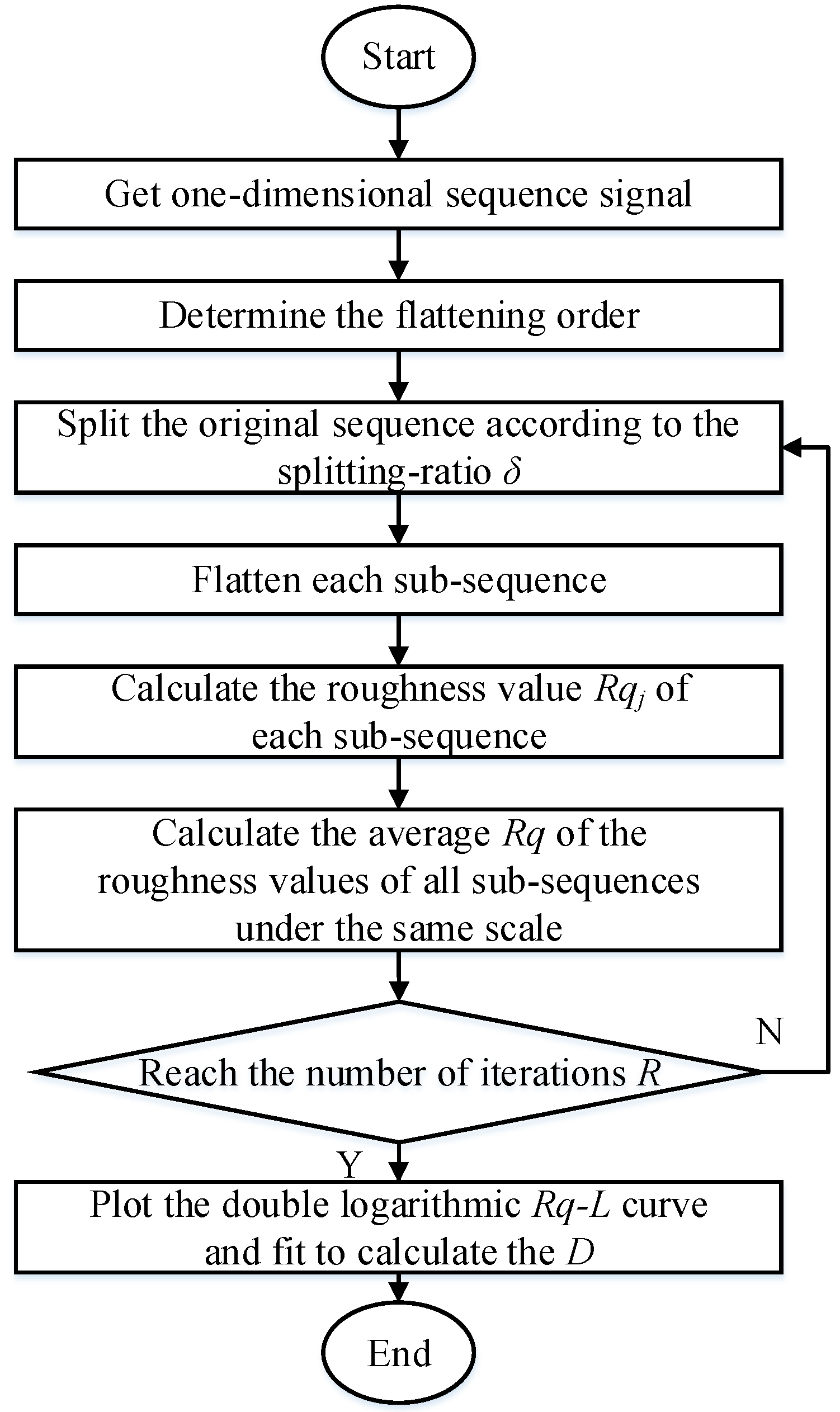
For each original sequence with N data points, L j , R q j value pairs are calculated as follows, and the flowchart of the RSE algorithm is shown in Figure 1.
First, the lengths of sub-sequence are defined as L 1 , L 2 , , L p , where L 1 = N , L p = 5 , L i = L i 1 × δ , i = 2, 3, …, p. The value of δ represents the reduction ratio of the sub-sequence length, which is 0.95 in this study. denoted the maximum integer value of the number in the brackets.
Second, the data pairs L j , R q j , j = 1 , 2 , , p are obtained. A starting point X ( r m ) in the original sequence is randomly determined, where r m means a random number, 1 r m N L j + 1 , j = 1 , 2 , , p . Then the sub-sequence with length L j is extracted out of the original sequence from the starting point, and thus the sub-sequence is composed of X ( r m ) , X ( r m + 1 ) , …, X ( r m + L j 1 ) .
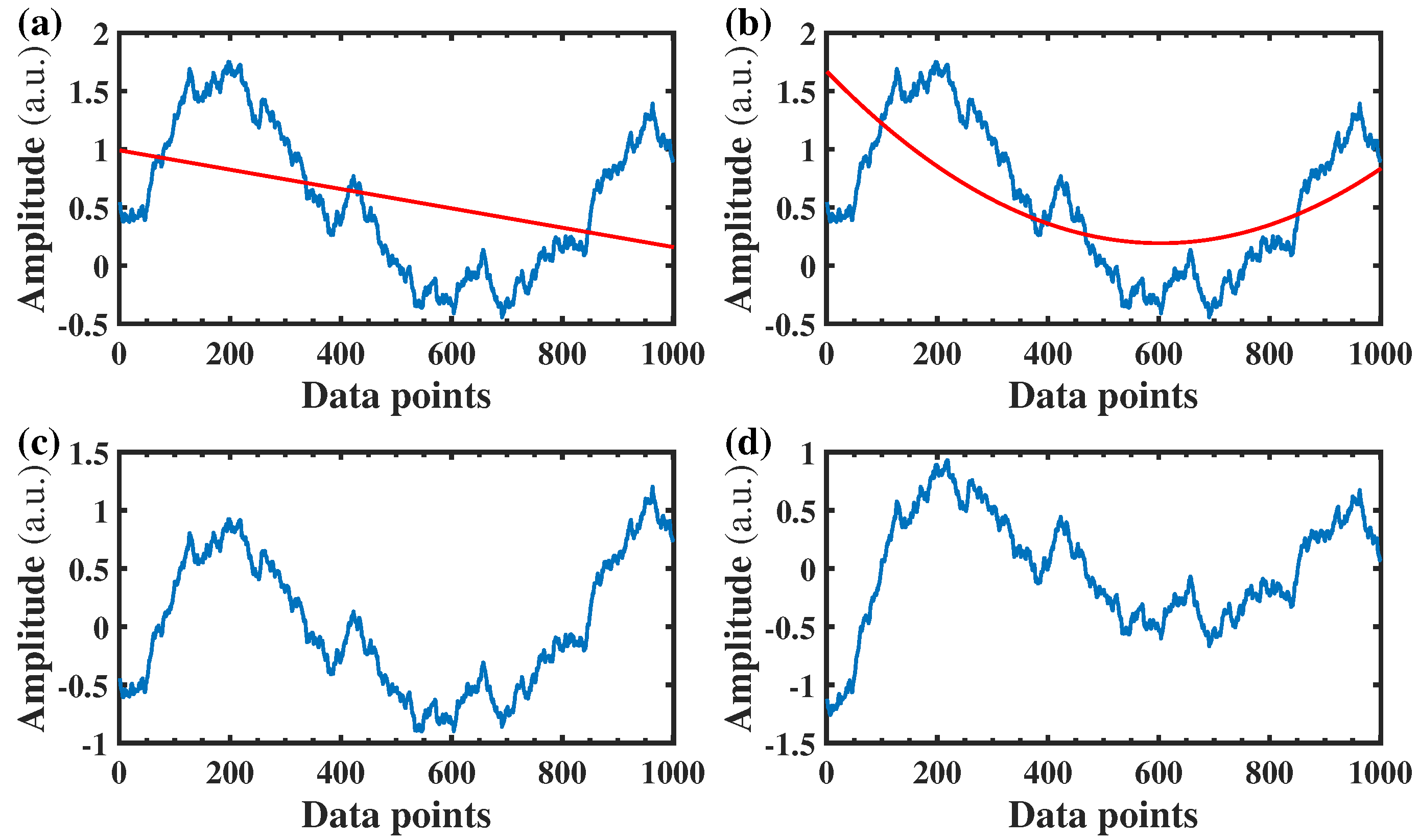
Third, the sub-sequences need to be flattened [25,37]. As shown in Figure 2, a polynomial fitting with a certain order (1 or 2 in this study) is performed on the sub-sequence, and the fitted polynomial is subtracted to obtain the flattened sub-sequence, which is used to calculate R q through Equation (2). The condition with flattening would be denoted as f0, and the flattening processes with 1-order and 2-orders would be denoted as f1 and f2, respectively.
Fourth, the above operation is repeated for R times ( R = 50 in this study) and the average values of R q of these sub-sequences are calculated as R q j . Therefore, a series of L j , R q j pairs could be obtained. If the original sequence has a fractal characteristic, the L j , R q j pairs would follow the power-law relationship shown in Equation (3) [39]. Meanwhile, the power-law relationship could enable a linear property under double-logarithm coordinates because of Equation (4), which could be fitted to obtain the value of D for a concerned profile.
R q = A L H = A L 2 D
ln R q = ( 2 D ) ln L + ln A

2.3. Scaling Region Interception

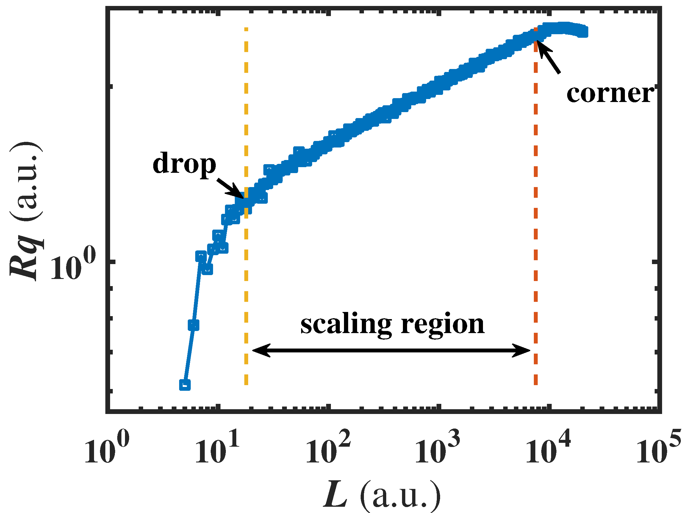
According to Figure 1, a typical R q -L curve obtained by the RSE operation with a 2-order flattening processing is illustrated in Figure 3. The deviation on the right (at larger L) would be named corner phenomenon, while that on the left (at smaller L), drop phenomenon. The location where the corner or drop began is defined as L c or L d . The linear part of the R q -L curve between L c and L d is the scaling region.
Due to the existence of corner and drop, the data fitting on the scaling region of R q -L curve is appropriate to acquire D rather than the global fitting on the entire curve. In our previous studies where the RSE algorithm was utilized, the data points which deviated from the scaling region were manually removed to carry out the fitting. However, the manual intervention might result in inaccuracy and inefficiency; thus, a scaling region interception method was used in this study.
This method was based on the characteristics of a scaling region in the R q -L curve, and the flowchart is shown in Figure 4. First, a polynomial f ( x ) is used to fit the entire R q -L curve. Second, the first and second derivatives ( f ( x ) and f ( x ) ) of the polynomial f ( x ) are obtained. Due to the linearity of the scaling region, the corresponding f ( x ) should be a constant in the region, while f ( x ) should be close to 0. Therefore, the scaling region is determined according to the first criterion of | f ( x ) | < δ 1 . The series of x values in the region are marked as l i , then the corresponding f ( x ) values are calculated and averaged to obtain f ( l i ) , which could be considered as the slope of the region. Since there are always fluctuations in the actual curves, the second criterion | ( f ( x ) f ( l i ) ) / f ( x ) | < δ 2 should also be met, and the obtained series of x values are L i , which should be a continuous segment corresponding to the targeted scaling region in the R q -L curve. In this study, δ 1 = 0.1 and δ 2 = 0.45 were used to determine L c and L d , thus identifying the scaling regions as shown in Figure 5.

2.4. Ideality Improvement of W-M Function

For the purpose of improving the ideality of the W-M function, a method that reduces the value of fundamental frequency γ n was proposed to achieve this goal. According to Equation (1), γ was set as 1.2 in this section. Because γ was a fixed value, decreasing the first item of n could have a positive effect on the ideality of the W-M function, thus taking the first item of n from 0 to −10, respectively, with an interval of −1. The position of drop and corner was calculated for different fractal dimensions D from 1.1 to 1.9 using the RSE algorithm, which was based on the scaling region interception method with 1-order flattening.

2.5. Modified Approach for Signal Simulation

In order to effectively simulate the acceleration signal of stable milling, the W-M function was modified. Equation (5) is the improved form of the W-M function. Where γ was also set as 1.2 in this section and the correction coefficient A of the W-M function is determined according to the value of the real signal R q -L curve on the right side of the corner. Let A = 1 and calculate the corresponding R q -L curve, then the value of R q on the right side of corner position is R q s i m . Equation (6) shows that correction coefficient A is the quotient of the R q r e a l , which is the value of the right of the corner position of the actual signal, and R q s i m , which is the value of the right of the corner position of the simulated signal. Furthermore, the value of D is the fractal dimension calculated by the real signal. Moreover, the maximum value of n is M ( M = 500 ), and the initial value of n is the position corresponding to the corner of the R q -L curve of the real signal, which is calculated by Equation (7), where f s is the sampling frequency, and L c is the position of the corner.
W ( x ) = n = C M A γ ( D 2 ) n cos φ n cos ( γ n x + φ n )
A = R q r e a l R q s i m
C = l o g γ 2 π f s L c

3. Results

3.1. Performances of R q -L Curves

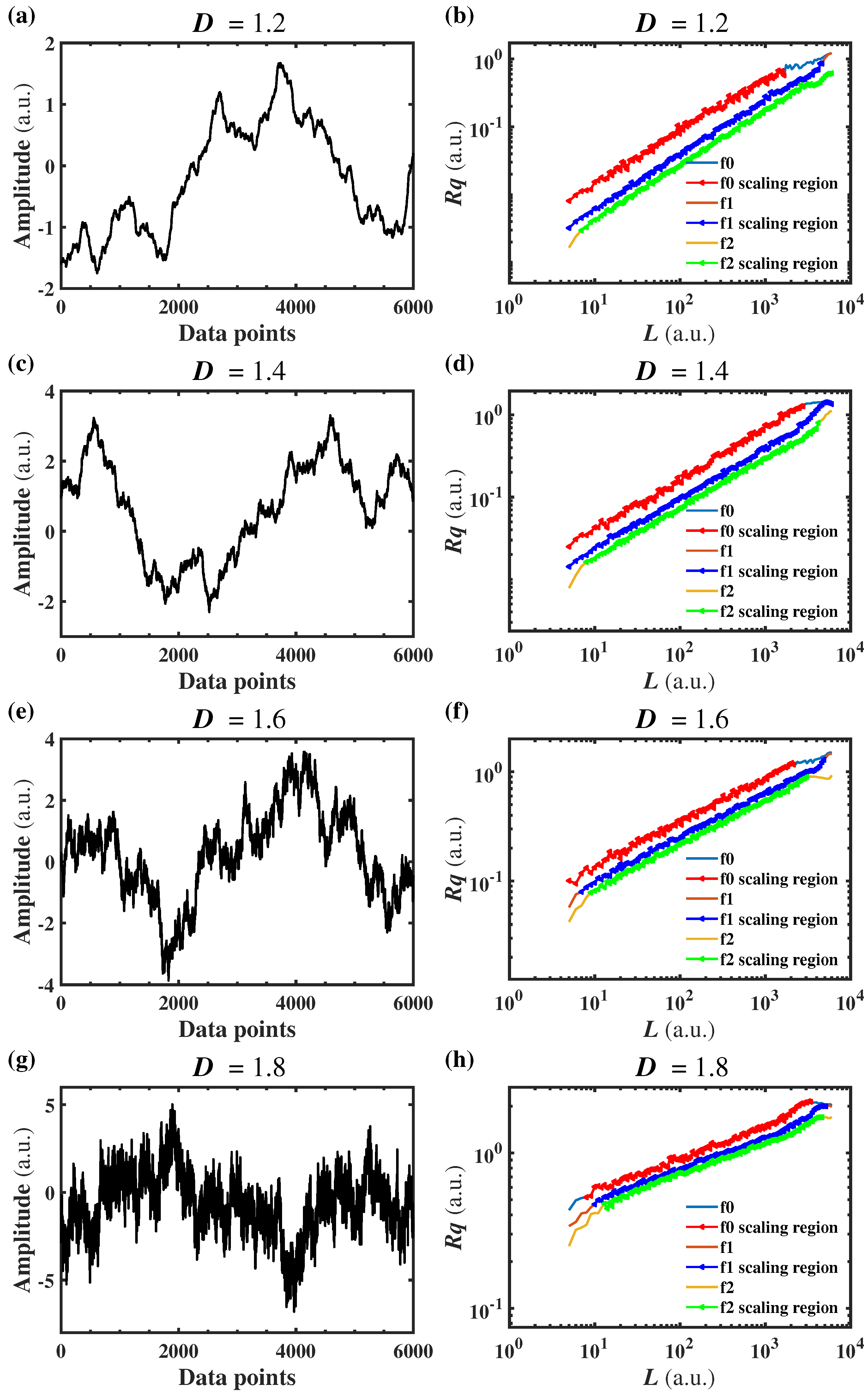
In Figure 6, the generated profiles could be observed together with their R q -L curves, whose scaling regions were denoted. Under various flattening orders, the scaling regions were generally parallel for each D, indicating that the calculated D values under different flattening orders would be close. Therefore, the quantified investigation into the influences of key factors on the RSE algorithm, such as sampling length and flattening order, would be carried out based on the R q -L curves.
As shown in Figure 6 and Figure 7, when the 1-order or 2-order flattening was used, the scaling region of the R q -L curve could be enlarged because L c increased along with the flattening order. Although there would be a drop phenomenon when higher flattening order was applied, its influence was much less than the corner because the variation of L d was much smaller than L c , which would be quantified in the section below. Compared to the situation of 0-order flattening, much more data points were in the scaling region and suitable for data-fitting; thus, the D calculation would be more accurate [25,37].
Except for flattening order, the other important factor influencing the scaling region is the sampling length. As could be observed in Figure 7, for each set of D and flattening order, the scaling region of R q -L curves increased along with the sampling lengths, and the scaling regions could overlap. Therefore, the scaling region could be extended by using a larger sampling length within a wide scope. However, such an enhancement would be limited when the sampling length is too large.
An essential fact relating to the above limitation is the lower critical condition of the W-M function, which is also critical to the corners of R q -L curves. Thus, it was added as a reference line denoted by a dotted line in Figure 7. When 0-order flattening was used, corners were always on the left side of the dotted line, indicating that the enhancement of the scaling region by using a larger sampling length would be limited by the lower critical condition. However, the corners for some curves of 1-order flattening and all curves of 2-order flattening could exceed the lower critical condition, which will be discussed below.
Moreover, when there were larger D and higher flattening orders, the drop phenomenon occurred. To quantify the influences of various parameters on the linearity of R q -L curves, an investigation into the positions of corner and drop ( L c and L d ) will be carried out.

3.2. Corner and Drop Properties

It could be found in Figure 8 that the sampling length and the flattening order played an important role in the position of the corner.
When sampling length increased, L c first increased almost linearly but then became stabilized. These two regions were linearly fitted, respectively. The intersection of fitted lines was defined as the sampling length stabilizing L c , which was summarized in Figure 8e.
As denoted as a dotted line in Figure 8, the lower critical condition limits L c to increasing along with sampling length only for 0-order flattening. As for 2-order flattening, the stabilized L c value could exceed such a limitation, indicating that the higher order of flattening in the RSE algorithm could enhance the linearity significantly by enlarging L c compared to 0-order flattening. For the flattening orders of 0, 1, and 2, the L c values which made sampling lengths stabilize were around 5197, 8222, and 10,562, respectively. They were approximately 0.81-fold, 1.28-fold, and 1.64-fold of the lower critical condition (6434), respectively. However, the above property of L c was not influenced obviously by D.
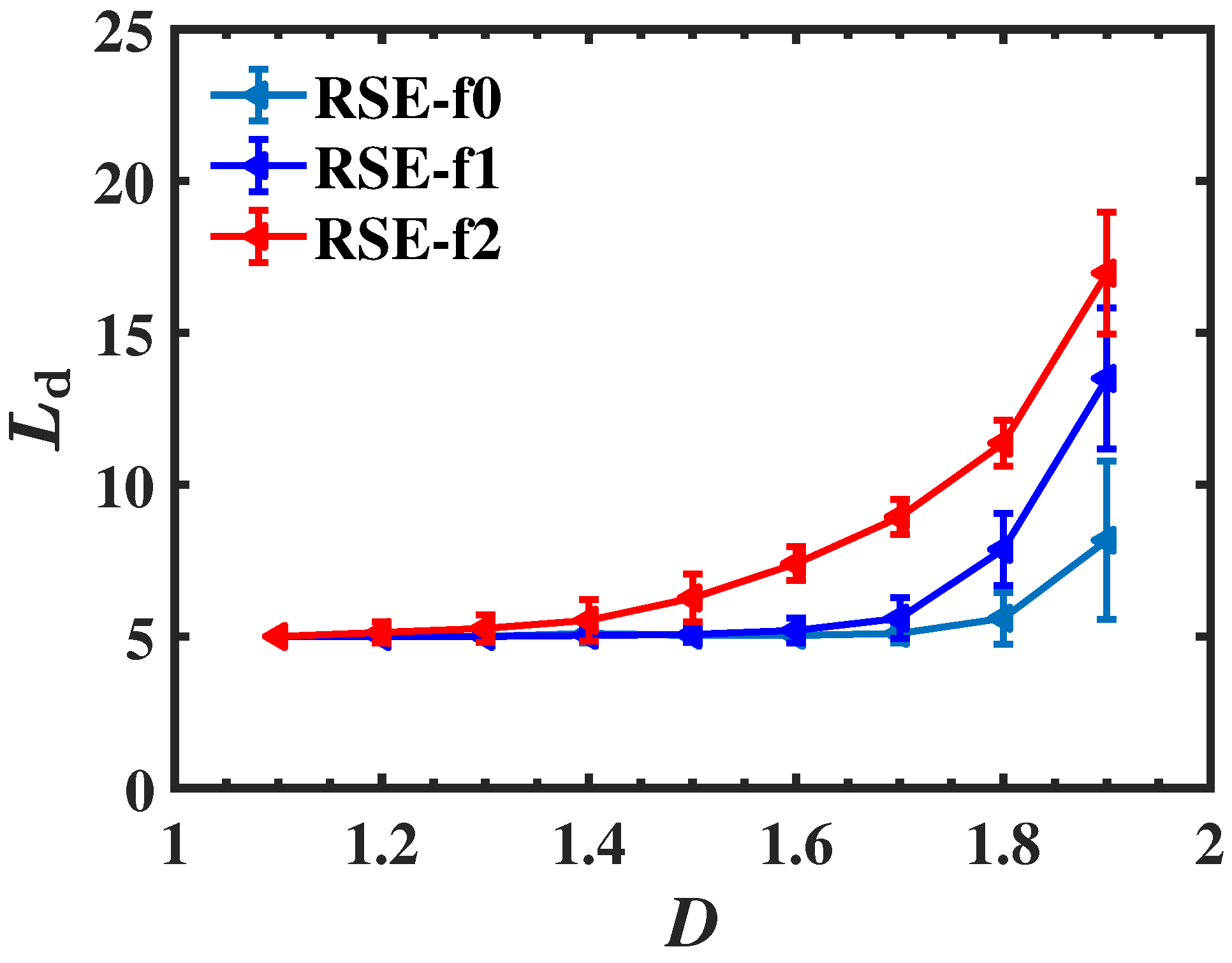
The position of the drop is influenced by the value of D and the flattening order. Figure 9 shows that the drop phenomenon began when D was raised above 1.5, and a higher flattening order made the value of L d larger. When there was no drop phenomenon in a R q -L curve, L d was recorded as 5.0, which was the minimum sub-sequence length used in this study. While the drop phenomenon began, the L d values were much lower (below 20) than the L c values shown in Figure 8. Therefore, the scaling region was generally determined by the corner, while the drop could not obviously affect the scaling region of the R q -L curve for a fractal profile. Consequently, the relationship between scaling region length and some factors such as sampling length and flattening order was similar to L c , as shown in Figure 8 and Figure 10.

3.3. RSE with Scaling Region Fitting

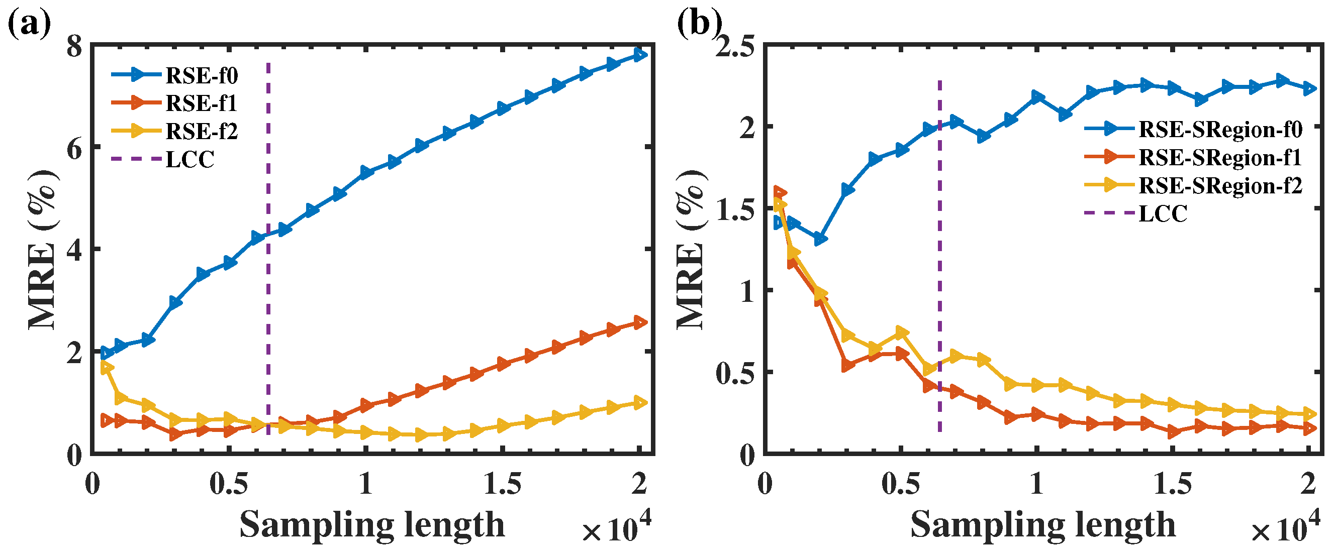
To verify the improvement by using the scaling region interception method, D values were calculated with and without the method. The D values were marked as D sr and D all respectively. The calculated D values ( D c ) were compared to the ideal fractal dimensions, which were generated by the W-M function ( D i ). Then, the mean relative error (MRE) was calculated according to Equation (8). All the results are illustrated in Figure 11, in which sub-figure (a) refers to D all , and (b) refers to D sr .
MRE = D c D i D i × 100 %
where represented the average operation.
When 0-order flattening was used, values of MRE without scaling region interception would increase along with the sampling length. The reason for this was that more data points out of the scaling region were involved in the fitting, which resulted in larger errors. However, when the scaling region interception was performed, the values of MRE increased gradually after the sampling length surpassed the lower critical condition and eventually stabilized. This was due to the elimination of data points from the scaling region before fitting. Thus, the error stabilized when the sampling length was sufficient.
When the 1-order or 2-order flattening was used without scaling region interception, values of MRE first decreased and then increased, which could also be attributed to the influence of sampling length on the scaling region, as shown in Figure 10. If scaling region interception was performed, values of MRE could be lowered by increasing the sampling length within a wide range and stabilized until the sampling length was much larger than the lower critical condition. Both MRE values of 1-order and 2-order flattening were much lower than those of 0-order flattening, which indicated that higher flattening order has significant accuracy.
In Figure 11a, the lowest MRE value was 0.37% (2-order flattening, under a sampling length of 12,000) and in Figure 11b, the lowest MRE value was only 0.13% (1-order flattening, under a sampling length of 15,000). Therefore, an optimized condition for the RSE algorithm with a scaling region interception method was obtained by using 1-order flattening and a sampling length of 15,000. Furthermore, it obviously showed that under the same flattening order and sampling length, the scaling region interception could improve the accuracy of the RSE algorithm significantly.

3.4. Corner Position of the Improved W-M Function

By analyzing the R q -L curves of the W-M function, it was found that the R q -L curves of the fractal profiles generated by the W-M function still had drop and corner phenomena, implying that the R q -L curves of the W-M function could not obtain an ideal scaling property. This phenomenon might be attributed to the fact that when Equation (1) was used, the initial value of n in Equation (1) was selected to be a certain integer number, e.g., 0 instead of to achieve the feasibility of practical calculation. Therefore, reducing the initial value of n made it more suitable for the condition of Equation (1). Figure 12 shows the changes of corner positions calculated by different fractal dimension D with different initial values of n, and more details about the positions of corner and drop are in Appendix A.
As shown in Figure 12, along with the decrease in the first item of n, the position of corners obtained by the scaling region interception method moved backward, which showed the same trend for different fractal dimension D, while the position of the drop showed a slight change, so that the scaling region length mainly depends on the change in corner position. Due to the variation of corner position, the scaling region is enlarged, which improves the scaling property of the W-M function in the whole domain.

3.5. Modified W-M Function for Signal Simulation

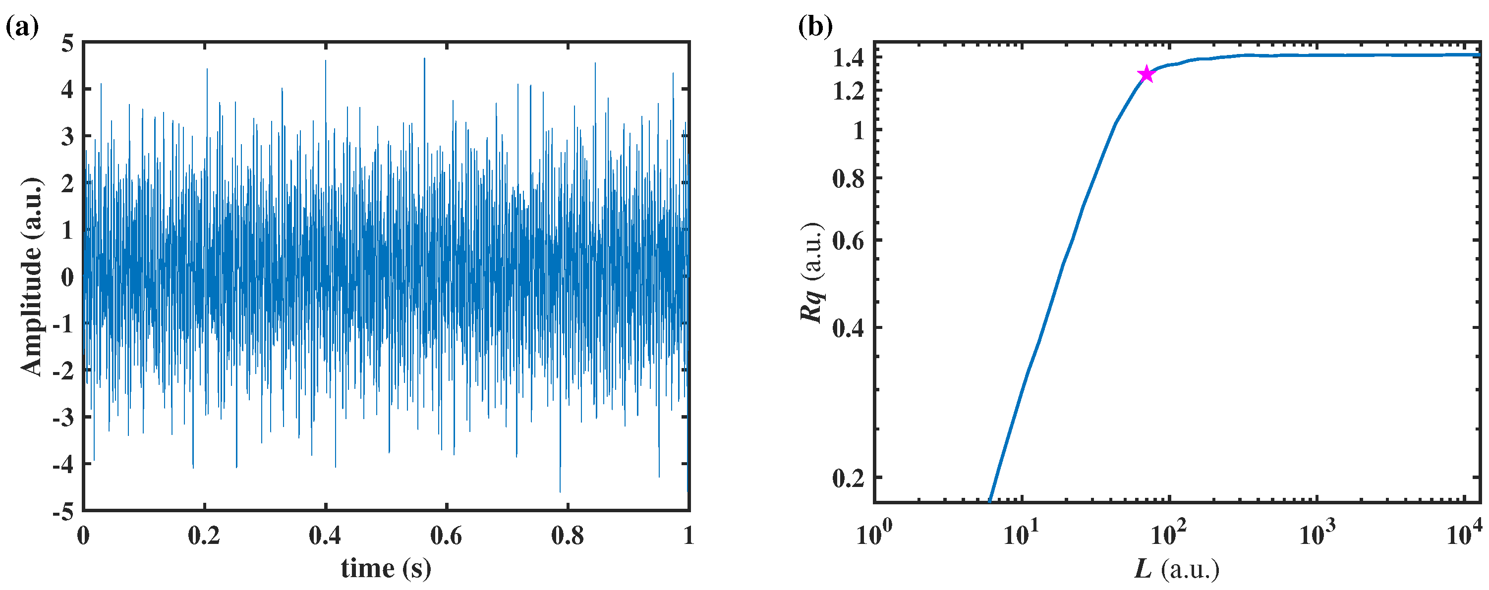
As shown in Figure 13a, the acceleration signal of 1 s stable milling was taken and was denoised by a five-order wavelet method. Figure 13b shows the R q -L curve of the signal obtained by using the RSE algorithm with 1-order flattening. By using the scaling region interception method, the corner position and fractal dimension D of the R q -L curve were obtained. It can be observed in Figure 13b that the corner position of the signal was (70, 1.35). On the right side of the corner, i.e., the non-fractal region where the value of R q no longer changed along with L, and the value of R q r e a l was 1.4168. When the correction coefficient A is equal to 1, the calculated R q s i m value was 0.00198, while the correction coefficient A based on (6) was 716. Based on the positions of the corner and drop extracted by the scaling region interception method, the fractal dimension D r e a l of the signal was 1.08. After obtaining the initial value of n by putting the abscissa of the corner of the real signal into Equation (7), a simulated signal could be generated by using a proper initial value of n, the correction coefficient A and the fractal dimension D r e a l into Equation (5).
Figure 14a,b illustrates the simulated signal generated by the modified W-M function and its R q -L curve, respectively. According to Figure 14a, the corner position of the generated signal was (70, 1.29) and the fractal dimension D s i m was 1.17. For the purpose of verifying the correctness of the simulated signal obtained by the modified W-M function, Figure 15 shows the comparison of R q -L curves of the real signal and the simulated signal. According to Equation (9), the relative error (RE) of the fractal dimension was 8.11%, where the D value of the real signal and simulated signal were marked as D r e a l and D s i m , respectively. Furthermore, the root-mean-square error (RMSE) of the two R q -L curves was 2.56%, which was calculated by Equation (10), where R q r i and R q s i represented the values of the real signal and simulated signal of R q , respectively. N was the number of R q . Based on the results of RE and RMSE, it was found that the modified W-M function could effectively simulate the machining signal.
R E = D s i m D r e a l D r e a l × 100 %
R S M E = i = 1 N ( R q r i R q s i ) 2 N × 100 %

4. Discussion

The application of the RSE algorithm with the scaling region interception method in the study of W-M function properties and scaling region length is of great significance. On the one hand, compared with our previous study [33,37], the results in Section 3.3 showed that the mean relative error between the fractal dimension calculated by the scaling region interception method and the ideal fractal dimension could be as low as 0.13%. Therefore, the calculation accuracy can be effectively improved. On the other hand, the RSE algorithm with the scaling region interception method is helpful in understanding the scaling regions of various forms and their properties. According to our latest paper [42], this method can be used for non-fractal research and is expected to have a deeper understanding of various nonlinear problems in nature.
Theoretically, the scaling region should be closely correlated to the lower critical condition because of the structure of the W-M function. As shown in Equation (1), a W-M function was superimposed by summing a series of cosine function terms, which enabled the scaling characteristics of the generated profile within a large scope of scale. However, the index of the first term could not be in the practical application of the W-M function; thus, its scaling characteristics could be compromised by the first cosine function with the lowest frequency, which determined the lower critical condition.
The first term in Section 2.1 was indexed as n = 0 , and the term expression was cos φ n cos x φ n , whose wavelength is equal to 2 π . If the concerned scope to analyze the property of the W-M function was defined as T, the surpassing T > T 0 = 2 π would lead to a repetition of the lowest-frequency information of 0 2 π in the scope beyond 2 π . If there was no item with a lower frequency, the fractal nature of the function could not be maintained. Therefore, to lead to more lowest-frequency information in the scope beyond the wavelength, reducing the first term could achieve this goal so that the ideality of the W-M function could be improved.
Such an approach to the lower critical condition could be reflected in the R q -L curves by the behavior of L c shown in Figure 8. Because L c L d , the length of the scaling region ( L c - L d ) is mainly determined by L c . Therefore, the relationship between lower critical condition and corner phenomenon should be analyzed. When the sampling length increased, L c was first raised and then stabilized; thus, the sampling length, which could stabilize L c was a critical parameter found in this study.
However, the sampling lengths that could stabilize L c are not equal to the length corresponding to the lower critical condition (LCC = 6434). Moreover, the flattening order has a significant influence, as shown in Table 1, where the average folds relative to LCC of the sampling lengths which could stabilize L c were 0.81, 1.28 and 1.64, respectively. When 0-order flattening was used, the stabilization of L c could occur if the sampling length was near LCC. While 1-order or 2-order flattening was used, the stabilization occurred after the sampling length surpassed LCC.
The above influence of the flattening order could enable an improvement in the accuracy of the RSE algorithm, as shown in Figure 11, because the sampling length that could stabilize L c could be enlarged by using the higher flattening order, which indicates a higher efficiency of sampling length. Moreover, there is another important reason for the accuracy improvement, which could be observed in the slope difference of the curves within the scope of small sampling lengths in Figure 10. The slopes are listed in Table 2, which could be summarized as the percentages of data points in the scaling region under flattening with 0-order, 1-order, and 2-order were 50%, 62% and 75%, respectively. Therefore, the efficiency of the sampling length is also significantly enhanced by increasing the flattening order, which improves the accuracy of data fitting to calculate D.
As for signal simulation, the key to the modified W-M function is to determine the index of the first term. According to Equation (7), the value of n corresponding to a point on the R q -L curve is inversely proportional to the abscissa of this point. Therefore, since the corner is a point to distinguish the fractal region and non-fractal region, the initial value of n of the simulated signal is determined by the value of n corresponding to the corner of a real signal, and then the lowest frequency is determined so that the R q -L curve of the simulated signal has the same corner position as the real signal. In addition, since the D value in Equation (5) was the D value of the real signal, the R q -L curve of the simulated signal and the real signal had the same slope on the left side of the corner. Moreover, the value of the correction coefficient A was adjusted so that the value of the right side of the corner of the R q -L curve for the simulated signal was the same as the real signal.
5. Conclusions

In this study, the properties of the scaling region of R q -L curves of profiles generated by the W-M function and influencing factors of scaling region length were investigated based on the RSE algorithm with a scaling region interception method. Then, it was verified that the proposed interception method can greatly improve the accuracy of fractal dimension D by the RSE algorithm. In addition, the ideality of the W-M function was improved. Moreover, we proposed a modified approach for signal simulation. The following conclusions are summarized as follows:
(1)
In the double logarithm coordinates, the majority of a R q -L curve of fractal profiles is linear. There are two types of data deviation out of the linear majority of the R q -L curve, i.e., the scaling region, which were named corner (at the right end) and drop (at the left end) phenomena, respectively.
(2)
The scaling region is generally determined by the location of corner phenomenon, i.e., L c . In addition, the drop phenomenon tended to occur for the profiles with higher D and a higher flattening order in the RSE operation. However, its influence on the scaling region is quite little compared with the corner.
(3)
The length of the scaling region is influenced by two main factors, which are the sampling length and flattening order, respectively. When the sampling length is increased, the scaling region length is first enlarged and then stabilized. The sampling length value, which could stabilize the scaling region length, is not close to LCC but is found to be 0.81, 1.28, and 1.64 folds of LCC when the flattening order is 0, 1, and 2, respectively.
(4)
By performing a scaling region interception method, the accuracy of the RSE algorithm could be improved significantly. Mean relative error could be as low as 0.13%. Particularly, when the flattening order is higher, the percentage of a scaling region within the sampling length is increased, representing a higher efficiency of data utilization.
(5)
By decreasing the initial value of n in the W-M function, the scaling region of the R q -L curve could be enlarged, and thus the ideality of the W-M function can be improved. When the initial value of n is lower, the value of the corner position becomes larger.
(6)
The acceleration signal of stable milling could be simulated by modifying the W-M function. Comparing R q -L curves of real signals with simulated signals, the RMSE of the two curves is 2.56%, demonstrating the feasibility of using the modified W-M function in simulating machining signals.

Author Contributions

Data curation, F.F., K.Z. and Y.X.; funding acquisition, P.F. and F.F.; investigation, K.Z., M.Y. and F.F.; project administration, X.L. and P.F.; visualization, K.Z. and Y.X.; writing—original draft, F.F. and K.Z.; writing—review and editing, X.L. and F.F. All authors have read and agreed to the present version of the manuscript.

Funding

This study was supported by the National Natural Science Foundation of China under Grant No. 51875311, Guangdong Basic and Applied Basic Research Foundation under Grant No. 2020A1515011199, and Shenzhen Natural Science Foundation under Grant No. WDZC20200817152115001.

Data Availability Statement

The data presented in this study are available from the corresponding author with a reasonable request. Moreover, the codes of analysis and simulation on fractal profiles and surfaces have been established, and the collaboration investigation by using them is welcome by the authors.

Acknowledgments

The authors would like to thank Shaozhu Xiao, Xiangsong Zhang, Binbin Liu, Shaocong Wang, Junlong Huang, Jun Li, Wenmeng Zhou and Zengxian Ma of Tsinghua University for their contributions to fractal studies in our lab.

Conflicts of Interest

The authors declare no conflict of interest.

Appendix A

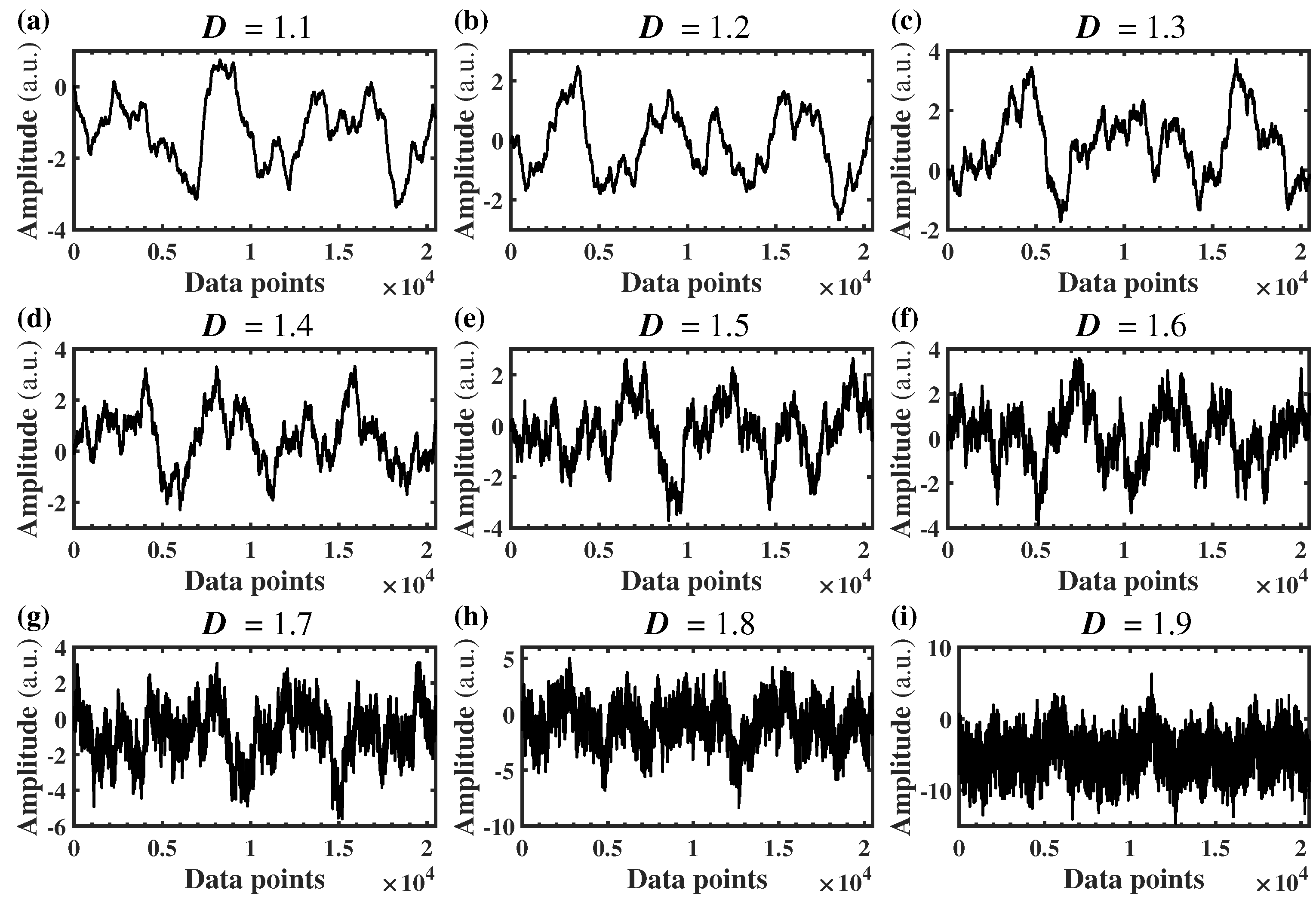
In this study, the ideal D values used in the W-M function ranged from 1.1 to 1.9, and the interval was 0.1. The sampling lengths were 500, 1000, 2000, …, 20,000. For each ideal D and sampling length, the calculation was repeated 30 times. The typical profiles of sequences with different D values generated through the W-M function are shown in Figure A1. The relevant data of corner and drop calculated by the RSE algorithm optimized with scaling region interception are listed in Table A1, Table A2, Table A3, Table A4, Table A5 and Table A6. Moreover, the positions of the corner and drop corresponding to different initial values of n are shown in Table A7 and Table A8.
Figure A1. The typical fractal profiles generated by using the W-M function.
Fractalfract 06 00542 g0a1
Table A1. Under all sampling lengths and all fractal dimensions, L c of corner points under the condition of 0-order flattening pre-processing.
Sampling LengthD
1.11.21.31.41.51.61.71.81.9
500350.0357.4336.9314.2312.7290.6240.4247.6264.3
1000713.0599.4635.3624.1586.5536.4426.1387.2465.8
20001344.41153.81130.01166.71103.0989.21076.0947.31046.7
30001737.91683.61766.91671.51545.81618.71676.81408.41059.6
40001745.82245.41999.22162.91840.02397.71883.52038.31897.2
50001870.82480.32355.02644.42248.62342.82434.92638.72148.9
60001976.62109.82509.52249.72456.02046.52472.22400.72255.7
70002116.82542.32115.72809.72583.22773.22542.12958.22583.4
80002135.72459.52428.42069.22833.72518.62525.82819.82730.9
90002267.32267.52224.92230.22501.12707.92853.92695.52613.4
10,0002125.82250.22365.62596.62765.82662.02763.92770.63322.4
11,0002133.12218.02447.62676.22409.62747.72740.93255.23024.5
12,0002215.52230.52399.42611.12580.62692.53024.62844.33053.8
13,0002245.72266.42488.22540.22487.02677.12894.82964.93128.2
14,0002291.62347.32310.42608.02546.92732.62958.62882.53043.9
15,0002221.12300.42311.12516.52556.32701.32854.62742.93156.3
16,0002190.92207.92292.92436.52490.42603.02710.72728.13111.3
17,0002199.12280.32340.62408.32488.22606.82772.82815.83050.9
18,0002202.92266.52194.82411.62479.52570.52790.82855.33249.1
19,0002327.72277.32261.52351.72435.02586.32785.82777.83106.6
20,0002177.52229.92221.02385.02530.82609.52754.62864.63149.4
Table A2. Under all sampling lengths and all fractal dimensions, L c of corner points under the condition of 1-order flattening pre-processing.
Sampling LengthD
1.11.21.31.41.51.61.71.81.9
500354.4337.9348.6325.2333.7307.2279.3274.3233.7
1000652.2672.4639.6704.1694.9614.6592.5513.4476.7
20001431.41271.11405.51343.71104.11157.01114.81199.91124.4
30001997.12242.92141.41978.42126.31930.71938.51678.91577.3
40002787.82728.42475.32605.82605.02805.42386.42565.42207.3
50002694.73477.93346.13540.63153.13268.43025.33602.82447.6
60003883.23845.23761.93928.53808.53244.04303.53838.83114.6
70003947.94831.24117.45053.94071.14792.84095.84888.53813.6
80004623.34800.55241.63959.85659.74783.65107.55016.34351.3
90005229.25311.34765.34920.95176.75971.04865.84744.64910.0
10,0004786.64452.54811.05201.35089.84892.65041.75337.55483.1
11,0004523.64705.54858.65170.64769.05154.94992.25790.55590.0
12,0004926.34671.35059.85225.35116.95152.75428.05269.35090.7
13,0004874.55050.35191.05260.35107.15113.75521.05353.55283.2
14,0005017.35117.65065.35567.15264.15467.65673.05364.15484.0
15,0004935.34977.94946.95385.65401.65460.45522.45312.05544.0
16,0004796.54915.85056.35232.25205.95372.35489.95281.65425.7
17,0004759.35007.55114.75379.55474.05308.35647.05342.05590.2
18,0004795.44833.04999.35394.55362.65199.45460.65414.05644.0
19,0004838.84857.64979.95314.15185.95312.95407.15275.35588.1
20,0004797.74853.04922.65172.15178.35260.55362.35278.65710.1
Table A3. Under all sampling lengths and all fractal dimensions, L c of corner points under the condition of 2-order flattening pre-processing.
Sampling LengthD
1.11.21.31.41.51.61.71.81.9
500392.7394.6360.0352.7376.8345.2357.5334.3314.8
1000781.0751.2634.4727.8732.0679.3692.7598.1506.0
20001604.61423.61537.61476.41427.01244.61375.51502.51222.5
30002089.72240.72122.92178.02150.32401.62095.52102.41848.6
40002975.32828.43069.72793.12828.92940.22685.72878.92464.4
50003336.64165.03672.54016.53455.53508.03750.63748.33448.4
60004655.34265.24458.94925.04106.14381.64503.74367.53740.3
70004846.35605.14982.46096.74411.85434.04659.75298.84197.2
80005642.56400.15990.15459.36520.25245.86158.15592.04874.1
90007521.87419.16780.56060.66722.26880.16653.56562.86205.4
10,0007473.27278.37507.07889.67982.77606.56941.46634.07416.2
11,0007540.57645.97507.18052.37771.18433.57671.58330.08114.5
12,0008055.37363.27606.88564.17740.07356.58050.07937.67553.3
13,0007621.28041.77913.38351.47666.37216.78407.67506.27453.5
14,0007794.27932.77283.78271.08282.88269.38276.87911.98002.1
15,0007721.07699.47408.18101.17854.98004.97801.58149.78498.7
16,0007638.47795.37818.27940.47977.28343.78513.78048.37555.4
17,0007729.87831.27800.08129.48203.98005.38230.07954.77557.7
18,0007775.47861.98010.88162.68159.88162.98176.28291.07638.2
19,0007780.77890.18023.28192.98236.98263.58173.38290.17832.8
20,0007819.97821.97959.98199.88118.38202.88174.28265.17958.6
Table A4. Under all sampling lengths and all fractal dimensions, L d of drop points under the condition of 0-order flattening pre-processing.
Sampling LengthD
1.11.21.31.41.51.61.71.81.9
5005.25.25.25.46.35.16.38.612.1
10005.15.15.05.25.15.15.26.18.8
20005.15.05.25.15.15.35.66.17.6
30005.15.05.15.15.15.15.25.78.3
40005.05.15.05.15.15.35.35.77.7
50005.15.05.15.15.05.25.25.58.9
60005.05.05.05.15.05.05.15.68.2
70005.15.05.15.05.05.05.35.78.0
80005.05.05.05.05.15.15.15.87.9
90005.05.15.15.15.05.15.15.88.7
10,0005.05.05.15.05.05.05.35.88.0
11,0005.05.15.05.05.05.15.15.68.5
12,0005.05.15.05.05.15.15.26.19.1
13,0005.05.05.05.05.15.15.25.58.4
14,0005.05.05.05.05.05.05.05.68.7
15,0005.05.05.05.05.15.15.25.69.6
16,0005.05.05.05.05.05.15.25.79.7
17,0005.05.05.05.05.05.05.15.810.9
18,0005.05.15.05.05.05.05.36.210.5
19,0005.05.05.15.15.15.05.35.79.8
20,0005.05.05.05.05.15.15.25.711.0
Table A5. Under all sampling lengths and all fractal dimensions, L d of drop points under the condition of 1-order flattening pre-processing.
Sampling LengthD
1.11.21.31.41.51.61.71.81.9
5005.05.25.05.05.15.35.69.210.7
10005.05.05.05.15.15.15.97.715.3
20005.05.05.05.05.15.26.17.911.9
30005.05.05.05.15.15.26.08.013.0
40005.05.05.05.05.05.25.67.613.0
50005.05.05.05.05.15.15.87.213.0
60005.05.05.05.05.15.25.67.913.5
70005.05.05.05.05.15.26.07.212.9
80005.05.05.05.05.15.25.97.913.0
90005.05.05.05.05.05.15.97.513.0
10,0005.05.05.05.05.05.25.37.812.8
11,0005.05.05.05.05.05.15.78.113.3
12,0005.05.05.05.05.05.25.88.112.8
13,0005.05.05.05.05.15.15.77.713.5
14,0005.05.05.05.05.05.15.87.713.6
15,0005.05.05.05.05.05.35.88.213.5
16,0005.05.05.05.05.15.16.27.913.8
17,0005.05.05.05.05.05.35.78.113.6
18,0005.05.05.05.05.05.15.68.113.6
19,0005.05.05.05.05.05.46.07.914.3
20,0005.05.05.05.05.05.36.28.015.0
Table A6. Under all sampling lengths and all fractal dimensions, L d of drop points under the condition of 2-order flattening pre-processing.
Sampling LengthD
1.11.21.31.41.51.61.71.81.9
5005.15.15.35.76.47.18.210.517.2
10005.05.35.25.56.27.18.510.916.7
20005.05.25.25.56.37.28.310.717.0
30005.05.15.35.46.17.28.511.216.7
40005.05.15.15.56.37.38.711.217.6
50005.05.15.25.46.27.48.611.317.1
60005.05.15.35.56.37.48.911.417.0
70005.05.15.25.66.47.38.811.616.6
80005.05.15.25.45.87.58.711.416.7
90005.05.05.25.76.27.18.911.817.0
10,0005.05.05.15.56.07.09.011.617.4
11,0005.15.15.25.36.27.18.911.917.3
12,0005.05.05.15.55.97.38.811.917.0
13,0005.05.05.25.56.17.38.911.917.5
14,0005.05.05.15.26.07.39.012.017.5
15,0005.05.05.15.35.97.59.212.018.4
16,0005.05.05.15.46.17.09.112.217.9
17,0005.05.05.25.26.27.39.212.217.9
18,0005.05.05.25.36.37.38.912.318.2
19,0005.05.05.25.46.27.28.812.418.4
20,0005.05.15.25.36.17.39.012.218.6
Table A7. L c of corner points under all initial values of n and all fractal dimensions.
nD
1.11.21.31.41.51.61.71.81.9
05418.94728.44066.43320.74502.24162.310,812.89103.17520.1
−15580.44738.54159.04026.75158.64681.211,478.29495.58759.9
−25786.85634.44720.94871.36147.45632.211,754.810,792.49533.7
−36888.46668.56208.55106.28136.910,965.812,046.011,586.011,979.1
−47255.06713.36774.89703.78782.511,273.013,325.513,837.512,015.6
−57671.37534.46826.510,313.811,469.113,834.115,132.514,581.512608.5
−68961.48318.66972.414,156.412,287.214,831.516,480.615,331.412,715.0
−710,555.49231.78928.514,369.612,410.620,621.617,745.416,501.115,622.7
−812,121.911,632.810,495.818,540.514,818.427,669.320,023.518,556.619,373.2
−912,692.513,314.010,919.421,977.919,815.529,104.327,302.326,388.322,504.6
−1019,924.316,345.513,154.932,729.323,051.135,283.730,629.032,008.829,215.4
Table A8. L c of drop points under all initial values of n and all fractal dimensions.
nD
1.11.21.31.41.51.61.71.81.9
05.05.05.05.05.05.36.28.015.0
−15.05.05.05.05.05.36.28.015.0
−25.05.05.05.05.05.36.28.015.0
−35.05.05.05.05.05.36.28.015.0
−45.05.05.05.05.05.36.28.015.0
−55.05.05.05.05.15.36.38.015.2
−65.05.05.05.05.05.46.48.115.0
−75.05.05.05.05.25.36.28.015.1
−85.05.05.05.05.15.56.38.215.3
−95.05.05.05.05.05.36.28.015.0
−105.05.05.05.05.15.46.28.215.1

References

  1. Mandelbrot, B. How Long Is the Coast of Britain? Statistical Self-Similarity and Fractional Dimension. Science 1967, 156, 636–638. [Google Scholar] [CrossRef]
  2. Mandelbrot, B. The Fractal Geometry of Nature; W. H. Freeman and Company: New York, NY, USA, 1977. [Google Scholar]
  3. Ma, Y.; Wang, Q.; Zhang, K. Average Distance of Sierpinski-Like Carpet. Fractals 2020, 29, 2150091. [Google Scholar] [CrossRef]
  4. Mandelbrot, B.B. Self-Affine Fractals and Fractal Dimension. Phys. Scr. 1985, 32, 257–260. [Google Scholar] [CrossRef]
  5. Kesić, S.; Spasić, S.Z. Application of Higuchi’s fractal dimension from basic to clinical neurophysiology: A review. Comput. Methods Programs Biomed. 2016, 133, 55–70. [Google Scholar] [CrossRef]
  6. Ziukelis, E.; Mak, E.; Dounavi, M.E.; Su, L.; O’Brien, J. Fractal dimension of the brain in neurodegenerative disease and dementia: A systematic review. Ageing Res. Rev. 2022, 79, 101651. [Google Scholar] [CrossRef]
  7. Qadri, M.; Namazi, H. Fractal-based analysis of the relation between tool wear and machine vibration in milling operation. Fractals 2020, 28, 2050101. [Google Scholar] [CrossRef]
  8. Namazi, H.; Farid, A.; Seng, C. Fractal based analysis of the variations of cutting forces along different axes in end milling operation. Fractals 2018, 26, 1850089. [Google Scholar] [CrossRef]
  9. Shi, C.T. Signal Pattern Recognition Based on Fractal Features and Machine Learning. Appl. Sci. 2018, 8, 1327. [Google Scholar] [CrossRef]
  10. Li, J.; Pelliciari, J.; Mazzoli, C.; Catalano, S.; Simmons, F.; Sadowski, J.T.; Levitan, A.; Gibert, M.; Carlson, E.; Triscone, J.M.; et al. Scale-invariant magnetic textures in the strongly correlated oxide NdNiO3. Nat. Commun. 2019, 10, 4568. [Google Scholar] [CrossRef]
  11. Xiao, Y.X.; Ying, J.; Tian, G.; Yang, X.; Zhang, Y.X.; Chen, J.B.; Wang, Y.; Symes, M.; Ozoemena, K.; Wu, J.; et al. Hierarchically Fractal PtPdCu Sponges and their Directed Mass- and Electron-Transfer Effects. Nano Lett. 2021, 21, 7870–7878. [Google Scholar] [CrossRef] [PubMed]
  12. Fu, J.; Jiao, J.; Song, H.; Gu, Z.; Liu, Y.; Geng, J.; Jack, K.S.; Du, A.; Tang, J.; Yu, C. Fractal-in-a-Sphere: Confined Self-Assembly of Fractal Silica Nanoparticles. Chem. Mater. 2020, 32, 341–347. [Google Scholar] [CrossRef]
  13. Suarez-Dominguez, E.J.; Perez-Rivao, A.; Sanchez-Medrano, M.T.; Perez-Sanchez, J.F.; Izquierdo-Kulich, E. Mesoscopic model for the surface fractal dimension estimation of solid-solid and gas-solid dispersed systems. Surfaces Interfaces 2020, 18, 100407. [Google Scholar] [CrossRef]
  14. Zhou, W.; Cao, Y.; Zhao, H.; Li, Z.; Feng, P.; Feng, F. Fractal Analysis on Surface Topography of Thin Films: A Review. Fractal Fract. 2022, 6, 135. [Google Scholar] [CrossRef]
  15. Cao, H.; Liu, L.; Wu, B.; Gao, Y.; Qu, D. Process optimization of high-speed dry milling UD-CF/PEEK laminates using GA-BP neural network. Compos. Part Eng. 2021, 221, 109034. [Google Scholar] [CrossRef]
  16. Spencer, K.L.; Wheatland, J.A.T.; Bushby, A.J.; Carr, S.J.; Droppo, I.G.; Manning, A.J. A structure-function based approach to floc hierarchy and evidence for the non-fractal nature of natural sediment flocs. Sci. Rep. 2021, 11, 14012. [Google Scholar] [CrossRef]
  17. Di Martino, G.; Iodice, A.; Riccio, D.; Ruello, G.; Zinno, I. The Role of Resolution in the Estimation of Fractal Dimension Maps From SAR Data. Remote Sens. 2018, 10, 9. [Google Scholar] [CrossRef]
  18. Yokoya, N.; Yamamoto, K.; Funakubo, N. Fractal-based analysis and interpolation of 3D natural surface shapes and their application to terrain modeling. Comput. Vision Graph. Image Process. 1989, 46, 284–302. [Google Scholar] [CrossRef]
  19. Wang, F.; Luo, C.; Chen, G. An improvement of G-P algorithm and its application. Chin. J. Comput. Phys. 1993, 10, 345–351. [Google Scholar]
  20. Tang, G.; Du, B.; Wang, S. Scaleless band automatic identification for fractal fault diagnosis of rotor system. J. Power Eng. 2009, 29, 440–444. [Google Scholar]
  21. Bolea, J.; Laguna, P.; Remartínez, J.; Rovira, E.; Navarro, A.; Bailón, R. Methodological Framework for Estimating the Correlation Dimension in HRV Signals. Comput. Math. Methods Med. 2014, 2014, 129248. [Google Scholar] [CrossRef]
  22. Chen, Z.; Liu, Y.; Zhou, P. A novel method to identify the scaling region of rough surface profile. Fractals 2018, 27, 1950011. [Google Scholar] [CrossRef]
  23. Zhou, S.; Wang, X.; Zhou, W.; Zhang, C. Recognition of the scale-free interval for calculating the correlation dimension using machine learning from chaotic time series. Phys. A Stat. Mech. Its Appl. 2022, 588, 126563. [Google Scholar] [CrossRef]
  24. Zuo, X.; Tang, X.; Zhou, Y. Influence of sampling length on estimated fractal dimension of surface profile. Chaos Solitons Fractals 2020, 135, 109755. [Google Scholar] [CrossRef]
  25. Wang, S.C.; Zhang, J.F.; Feng, F.; Qian, X.; Jiang, L.Q.; Huang, J.L.; Liu, B.B.; Li, J.; Xia, Y.S.; Feng, P.F. Fractal Analysis on Artificial Profiles and Electroencephalography Signals by Roughness Scaling Extraction Algorithm. IEEE Access 2019, 7, 89265–89277. [Google Scholar] [CrossRef]
  26. Higuchi, T. Approach to an Irregular Time-Series on the Basis of the Fractal Theory. Phys. D-Nonlinear Phenom. 1988, 31, 277–283. [Google Scholar] [CrossRef]
  27. Katz, M.J. Fractals and the analysis of waveforms. Comput. Biol. Med. 1988, 18, 145–156. [Google Scholar] [CrossRef]
  28. Zhang, X.; Xu, Y.; Jackson, R.L. An analysis of generated fractal and measured rough surfaces in regards to their multi-scale structure and fractal dimension. Tribol. Int. 2017, 105, 94–101. [Google Scholar] [CrossRef]
  29. Liebovitch, L.S.; Toth, T. A Fast Algorithm to Determine Fractal Dimensions by Box Counting. Phys. Lett. A 1989, 141, 386–390. [Google Scholar] [CrossRef]
  30. Ponomareva, A.A.; Moshnikov, V.A.; Suchaneck, G. Evaluation of the fractal dimension of sol-gel deposited oxide films by means of the power spectral density. Glass Phys. Chem. 2014, 40, 203–207. [Google Scholar] [CrossRef]
  31. Wang, G.; Wang, L.; Yuan, Y. Investigation on Dynamics Performance of Multibody System with Rough Surface. Appl. Math. Model. 2021, 104, 358–372. [Google Scholar] [CrossRef]
  32. Zhifang, Z.; Yang, Y.; Han, H.; Ma, H.; Wang, H.; Li, Z.W. Meshing Characteristics of Spur Gears Considering Three-Dimensional Fractal Rough Surface under Elastohydrodynamic Lubrication. Machines 2022, 10, 705. [Google Scholar] [CrossRef]
  33. Feng, F.; Huang, J.; Li, X.; Qu, T.; Liu, B.; Zhou, W.; Qian, X.; Feng, P. Influences of planarization modification and morphological filtering by AFM probe-tip on the evaluation accuracy of fractal dimension. Surf. Coatings Technol. 2019, 363, 436–441. [Google Scholar] [CrossRef]
  34. Majumdar, A.; Tien, C. Fractal characterization and simulation of rough surfaces. Wear 1990, 136, 313–327. [Google Scholar] [CrossRef]
  35. Berry, M.V. On the Weierstrass-Mandelbrot fractal function. Proc. R. Soc. Lond. A Math. Phys. Sci. 1997, 370, 459–484. [Google Scholar] [CrossRef]
  36. Zhu, H.; Ge, S.; Huang, X.; Zhang, D.; Liu, J. Experimental study on the characterization of worn surface topography with characteristic roughness parameter. Wear 2003, 255, 309–314. [Google Scholar] [CrossRef]
  37. Feng, F.; Liu, B.B.; Zhang, X.S.; Qian, X.; Li, X.H.; Huang, J.L.; Qu, T.M.; Feng, P.F. Roughness scaling extraction method for fractal dimension evaluation based on a single morphological image. Appl. Surf. Sci. 2018, 458, 489–494. [Google Scholar] [CrossRef]
  38. Feng, F.; Shi, K.; Xiao, S.; Zhang, Y.; Zhao, Z.J.; Wang, Z.; Wei, J.J.; Han, Z. Fractal analysis and atomic force microscopy measurements of surface roughness for Hastelloy C276 substrates and amorphous alumina buffer layers in coated conductors. Appl. Surf. Sci. 2012, 258, 3502–3508. [Google Scholar] [CrossRef]
  39. Kulesza, S.; Bramowicz, M. A comparative study of correlation methods for determination of fractal parameters in surface characterization. Appl. Surf. Sci. 2014, 293, 196–201. [Google Scholar] [CrossRef]
  40. Zhou, W.; Li, X.; Feng, F.; Qu, T.; Huang, J.; Qian, X.; Zha, H.; Feng, P. Robustness of Surface Roughness against Low Number of Picture Elements and Its Benefit for Scaling Analysis. Coatings 2020, 10, 776. [Google Scholar] [CrossRef]
  41. Li, Z.; Qian, X.; Feng, F.; Qu, T.; Xia, Y.; Zhou, W. A continuous variation of roughness scaling characteristics across fractal and non-fractal profiles. Fractals 2021, 29, 2150109. [Google Scholar] [CrossRef]
  42. Li, Z.; Wang, J.; Yuan, M.; Wang, Z.; Feng, P.; Feng, F. An indicator to quantify the complexity of signals and surfaces based on scaling behaviors transcending fractal. Chaos Solitons Fractals 2022, 163, 112556. [Google Scholar] [CrossRef]
  43. Gou, X.; Schwartz, J. Fractal analysis of the role of the rough interface between Bi2Sr2CaCu2Oxfilaments and the Ag matrix in the mechanical behavior of composite round wires. Supercond. Sci. Technol. 2013, 26, 055016. [Google Scholar] [CrossRef]
Figure 1. The operation flowchart of the RSE algorithm.
Fractalfract 06 00542 g001
Figure 2. An example of the flattening process: The original profile (blue line) and the fitted polynomial line (red line) with (a) 1-order, (b) 2-order; the flattened profile by subtracting the polynomial with (c) 1-order, (d) 2-order.
Fractalfract 06 00542 g002
Figure 3. A typical R q -L curve obtained by the RSE operation with 2-order flattening processing, where D and the sampling length were 1.9 and 20,000, respectively.
Fractalfract 06 00542 g003
Figure 4. The operation flowchart of the scaling region interception method.
Fractalfract 06 00542 g004
Figure 5. The typical R q -L curves obtained by the RSE algorithm with 2-order flattening and sampling length of 6000 and the corresponding derivatives: (a,b) D = 1.1; (c,d) D = 1.5; (e,f) D = 1.9. The scaling regions obtained by the proposed scaling region interception method were plotted by using red triangle symbols.
Fractalfract 06 00542 g005
Figure 6. At the same sequence length 6000, different fractal dimensions of the original curve and the performance of the scaling region interception method under 0, 1, and 2 order flattening pre-processing conditions. (a,b) D = 1.2; (c,d) D = 1.4; (e,f) D = 1.6; (g,h) D = 1.8.
Fractalfract 06 00542 g006
Figure 7. The typical R q -L curves when the sampling length was 500, 5000, 10,000, 15,000. The flattening order was varied (0, 1 or 2) in the calculation by using the RSE algorithm, and the lower critical condition (LCC, at L = 6434) of the W-M function was denoted as a dashed line for reference. (ac) D = 1.2 with different flattening order and sampling length; (df) D = 1.4 with different flattening order and sampling length; (gi) D = 1.6 with different flattening order and sampling length; (jl) D = 1.8 with different flattening order and sampling length.
Fractalfract 06 00542 g007
Figure 8. Typical relationship curves between the position of corner ( L c ) and sampling length under various flattening orders: (a) D = 1.2, (b) D = 1.4, (c) D = 1.6, (d) D = 1.8. (e) The sampling lengths that could stabilize L c when D ranged from 1.1 to 1.9. (f) The average folds relative to LCC of the sampling lengths, which could stabilize L c .
Fractalfract 06 00542 g008
Figure 9. The average L d values under various flattening orders and D.
Fractalfract 06 00542 g009
Figure 10. The relationships between scaling region length (SRL) and the sampling length under the flattening order of: (a) 0, (b) 1, (c) 2. (d) The influence of flattening orders on the sampling length that could stabilize SRL.
Fractalfract 06 00542 g010
Figure 11. Variation of the mean relative error (MRE) and mean square error (MSE) with the sampling length and flattening order. (a) MRE obtained by using the RSE algorithm without scaling region interception, (b) MRE with scaling region interception.
Fractalfract 06 00542 g011
Figure 12. The change in corner position under different D values and n values. (a) D = 1.1, (b) D = 1.2, (c) D = 1.3, (d) D = 1.4, (e) D = 1.5, (f) D = 1.6, (g) D = 1.7, (h) D = 1.8, (i) D = 1.9.
Fractalfract 06 00542 g012
Figure 13. (a) The acceleration signal of 1s stable milling, (b) the R q -L curve of the acceleration signal and the star is the position of corner.
Fractalfract 06 00542 g013
Figure 14. (a) The simulated signal, (b) the R q -L curve of the simulated signal and the star is the position of corner.
Fractalfract 06 00542 g014
Figure 15. The comparison of R q -L curves of the actual signal and the simulated signal.
Fractalfract 06 00542 g015
Table 1. The sampling length stabilizing L c data.
D = 1.1D = 1.2D = 1.3D = 1.4D = 1.5
RSE-f03269.064245.544571.354612.415741.10
RSE-f18421.237157.128000.008357.008000.00
RSE-f210,250.579388.5510,000.0011,212.0510,233.97
D = 1.6 D = 1.7 D = 1.8 D = 1.9Folds
RSE-f04334.935343.945376.869276.560.81
RSE-f18584.098000.007589.289891.821.28
RSE-f210,468.0711,465.0311,000.0011,044.131.64
Table 2. The increasing range slopes of Figure 10.
D1.11.21.31.41.51.61.71.81.9Mean
RSE-f00.560.540.490.530.430.590.490.540.300.50
RSE-f10.560.680.600.590.640.620.640.710.550.62
RSE-f20.760.820.750.740.770.750.720.710.730.75
Publisher’s Note: MDPI stays neutral with regard to jurisdictional claims in published maps and institutional affiliations.