Global Bifurcation Behaviors and Control in a Class of Bilateral MEMS Resonators

Abstract

The investigation of global bifurcation behaviors the vibrating structures of micro-electromechanical systems (MEMS) has received substantial attention. This paper considers the vibrating system of a typical bilateral MEMS resonator containing fractional functions and multiple potential wells. By introducing new variations, the Melnikov method is applied to derive the critical conditions for global bifurcations. By engaging in the fractal erosion of safe basin to depict the phenomenon pull-in instability intuitively, the point-mapping approach is used to present numerical simulations which are in close agreement with the analytical prediction, showing the validity of the analysis. It is found that chaos and pull-in instability, two initial-sensitive phenomena of MEMS resonators, can be due to homoclinic bifurcation and heteroclinic bifurcation, respectively. On this basis, two types of delayed feedback are proposed to control the complex dynamics successively. Their control mechanisms and effect are then studied. It follows that under a positive gain coefficient, delayed position feedback and delayed velocity feedback can both reduce pull-in instability; nevertheless, to suppress chaos, only the former can be effective. The results may have some potential value in broadening the application fields of global bifurcation theory and improving the performance reliability of capacitive MEMS devices.

1. Introduction

Electrostatic microresonators have attracted significant attention thanks to their wide applications in micro-electromechanical systems (MEMS) such as micro sensors [1], micro filters [2], and energy harvesters [3]. To maintain their normal work performance, harmonic vibration is desirable. However, due to nonlinearities in the driven force, stiffness, damping [4] and structural geometry [5], the vibrating structures of MEMS resonators do not necessarily undergo periodic responses. During these decades, sufficient works have studied the conditions for achieving stable periodic responses. Hajjaj et al. [6] investigated different types of internal resonances of an electrostatic MEMS arch resonator via the theory of local bifurcation and experiments. Ali and Ardeshir [7] modeled a dielectric elastomer resonator as a sandwiched Euler-Bernoulli microbeam and presented multiple periodic responses induced by subcritical bifurcations. Zhu and Shang [8] discussed the phenomenon jump among coexisting multiple periodic attractors in an electrostatic bilateral microresonator. It has been realized that even if MEMS resonators finally vibrate periodically, the phenomenon jump among coexisting multiple periodic attractors is unwanted as it leads to unreliability of work performance of the micro devices.

Apart from multistability, there are some other initial-sensitive dynamic behaviors of micro resonators, for instance, chaos and pull-in instability. The former is well-known in nonlinear dynamic systems [9,10,11], whereas the latter is a unique phenomenon of electric-actuated capacitive micro devices. The phenomenon pull-in instability is related to but different from the behavior pull in. The latter describes a movable electrode collapsing to a rigid one [12] thus implying an unbounded or escape solution of the corresponding dynamic systems [13]. It is unfavorable in MEMS resonators for causing the failure of their performance. Pull-in instability means that a subtle disturbance of initial state causes a sudden change of dynamic behavior from bounded dynamic responses to pull in. It is similar to the phenomenon of frequency jump. It is also an unwanted dynamic behavior since it implies the loss of global integrity and performance reliability of the concerned MEMS devices [14,15].

For chaos and its control of MEMS resonators, there have been significant works in recent years. Fu and Xu [16] considered the application of a single-side MEMS resonator in pressure detecting and numerically studied critical conditions for multi-field parameters for inducing chaos. For a single-side arch micro/nano resonator, Liu et al. [17] introduced delayed velocity feedback to restrain frequency jump as well as chaos and discussed the control effect numerically. For double-side micromechanical resonators, as there are multiple potential wells in their vibrating systems, chaos is easily triggered by homoclinic bifurcations [18,19,20]. Luo et al. [18] studied the observer-based adaptive stabilization issue of the fractional-order chaotic MEMS resonator with uncertain functions via numerical simulations. Haghighi and Markazi [19] predicted the transient chaos of another type of bilateral MEMS resonator by the approximately analytical criterion of homoclinic bifurcation and then proposed a robust adaptive fuzzy control algorithm to suppress it. Siewe and Hegazy [20] found that chaos could be induced by both homoclinic and heteroclinic bifurcation which was confirmed by numerical simulations of basins of attraction and bifurcation diagrams. Due to the electrostatic-driven forces of MEMS resonators, the dynamic systems of these MEMS resonators contain fractional functions, which cause the difficulty of analyzing homoclinic bifurcation by classical bifurcation theory. In most studies, homoclinic bifurcation is discussed by expanding the fractal functions approximately in Taylor’s series as third-order [19] or fifth-order [20] polynomials, thus it has some limitations in the values of system parameters such as DC voltage. When it comes to heteroclinic bifurcation, this theoretical method cannot work.

The phenomenon pull-in instability is still relatively little considered in the literature. For the vibrating system of a single-side MEMS resonator, Alsaleem et al. [21] applied the erosion of safe basin to depict pull-in instability numerically, proposed delayed feedback to suppress this phenomenon, and studied the control effect experimentally and numerically. On this basis, Shang [22] studied the mechanism of pull-in instability and its control in this system and found that it is induced by homoclinic bifurcation, and that the two types of delayed controllers were both useful for a positive coefficient of the gain and a short delay. For the MEMS resonator actuated by two-sided electrodes, Gusso et al. numerically illustrated its rich nonlinear dynamics such as multistability, pull-in instability and chaos [23].

As shown in the above research, chaos and pull-in instability are both global bifurcation behaviors. Two questions are raised: Is there any relationship between chaos and pull-in instability? Can a control strategy reduce both of them? To answer these questions, we considered a typical bilateral MEMS resonator containing multiple potential wells [8,19], and investigated the mechanisms behind chaos and pull-in instability of MEMS resonators as well as the mechanisms of control strategies on reducing them. The rest of the paper is arranged as follows. In Section 2, the dynamic model of the MEMS resonator and its static bifurcation is discussed. In Section 3, global bifurcation and induced behaviors are analyzed. In Section 4, two control strategies, namely, delay position feedback and delay velocity feedback, are applied to the original system respectively; and their control mechanisms and effect on the global bifurcation behavior are studied in detail. Section 5 contains the discussion.

2. Mathematical Model and Unperturbed Dynamics

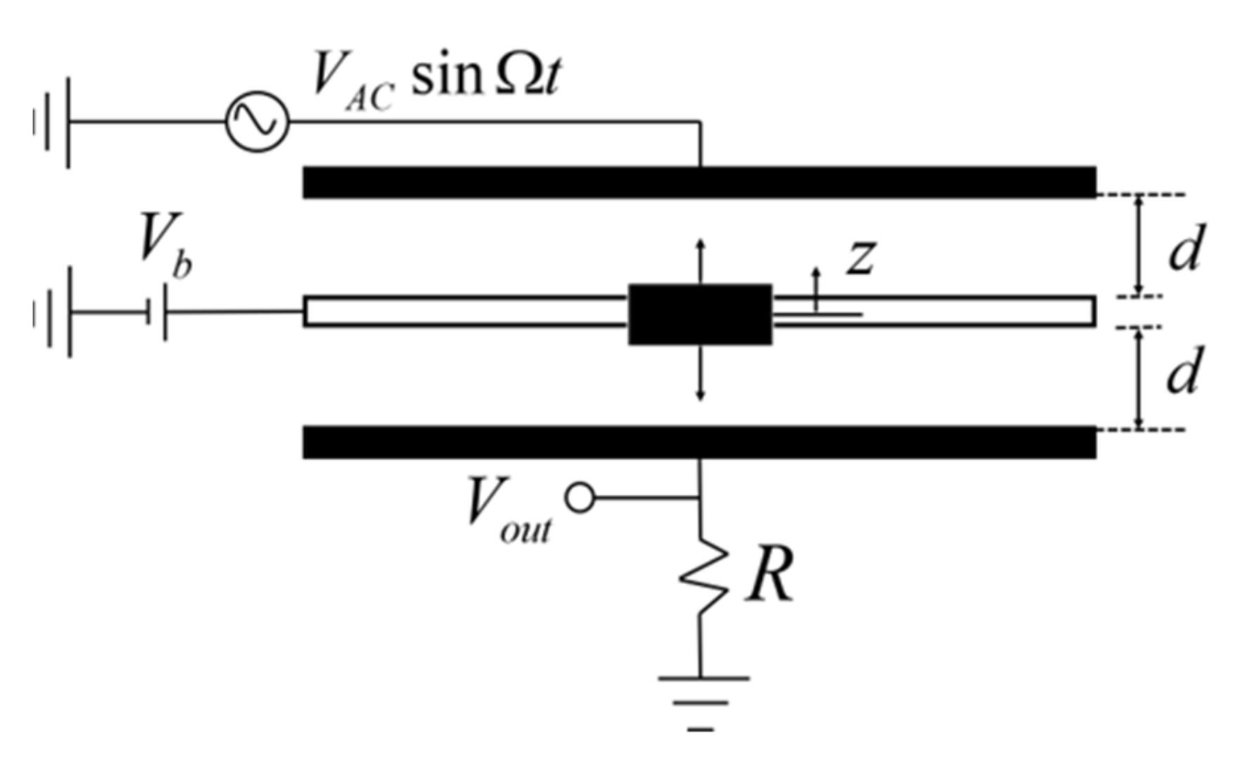
The schematic diagram of a typical bilateral MEMS resonator is depicted in Figure 1. The MEMS resonator consists of the movable electrode and nonlinear electrostatic forces on each side [8,19]. In this system, an external driving force on the resonator is applied by means of electrical driving voltages. According to the Second Law of Newton, the governing differential equation of motion for this MEMS resonator can be expressed as

$$m\frac{{\mathrm{d}}^{2}z}{\mathrm{d}{t}^2}+c\frac{\mathrm{dz}}{\mathrm{d}t}+k_{1}z+k_3{z}^3=F_e^u+F_e^l,$$

(1)

where $F_e^u$ and $F_e^l$ are the electrostatic forces from the upper and the lower capacitor in Figure 1, respectively. As they are driven by the combined voltage, which is made up of a DC bias voltage and an AC voltage, they can be described as [12,19]

$$F_e^u=\frac{A_0}{2{(d-z)}^2}{(V_b+V_{AC}\sin \mathrm{\Omega }t)}^2,\hspace{1em}{F}_e^l=-\frac{A_0{V}_b^2}{2{(d+z)}^2}.$$

(2)

Figure 1. Simplified diagram of a bilateral electrostatic micro resonator.

The nomenclatures of the system parameters in Equations (1) and (2) are presented in Table 1.

Table 1. Parameters of systems (1) and (5).

Parameter	Symbol
Equivalent mass of the proof mass (kg)	m
Viscous damping coefficient in the high vacuum environment (N·s/m)	c
Linear stiffness coefficient (N/m)	$k_1$
Cubic stiffness term (N/m3)	$k_3$
Capacitance of each parallel plate at rest ($\mathrm{Fm}$)	$A_0$
Initial gap width between the two neighboring parallel plates (m)	d
DC bias voltage (V)	$V_b$
Frequency of AC voltage (HZ)	Ω
Amplitude of AC voltage (V)	$V_{AC}$
Time	t
Displacement of the proof mass at time t	$z$

By introducing the dimensionless time $T={\omega }_{0}t$ where ${\omega }_0=\sqrt{\frac{k_1}{m}}$, and the variable $x(T)=\frac{z}{d}$, the dimensionless form of Equation (1) can be expressed by

$$x^{″}(T)+\mu x^{\prime }(T)+x+\alpha x^3=\frac{\beta }{{\left(1-x\right)}^2}{\left(1+\gamma \sin (\omega T)\right)}^2-\frac{\beta }{{\left(1+x\right)}^2}.$$

(3)

where

$$\omega =\frac{\mathrm{\Omega }}{{\omega }_0},\mu =\frac{c}{m{\omega }_0},\alpha =\frac{k_3{d}^2}{m{\omega }_0^2},\beta =\frac{A_0{V}_b^2}{2k_1{d}^3},\gamma =\frac{V_{AC}}{V_b}$$

(4)

Denoting $x(T)\triangleq x,\hspace{1em}{x}^{\prime }(T)\triangleq \dot{x},\hspace{1em}{x}^{″}(T)\triangleq \ddot{x}$ in Equation (3) yields the following dimensionless system

$$\ddot{x}+\mu \dot{x}+x+\alpha x^3=\frac{\beta }{{\left(1-x\right)}^2}{\left(1+\gamma \sin (\omega T)\right)}^2-\frac{\beta }{{\left(1+x\right)}^2}.$$

(5)

The variable x in Equation (5) should satisfy |x| ≤ 1. Note that |x| = 1 shows the gap width between the movable electrode and one of its neighboring fixed electrodes being zero, thus creating the phenomenon pull in. Since the viscous-damping coefficient c is tiny, and V_AC << V_b, the parameters μ and β in Equation (5) are both small, the concerned terms can be considered as the perturbed ones. Thus, the unperturbed system of Equation (5) is

$$\dot{x}=y,\hspace{1em}\dot{y}=-x-\alpha x^3+\frac{\beta }{{(1-x)}^2}-\frac{\beta }{{(1+x)}^2}$$

(6)

which is a Hamiltonian system with the Hamiltonian [19]

$$H\left(x,y\right)=\frac{1}{2}{x}^2+\frac{1}{2}{y}^2+\frac{\alpha }{4}{x}^4-\frac{\beta }{1-x}-\frac{\beta }{1+x}+2\beta .$$

(7)

According to Equations (6) and (7), the existence, shapes and positions of potential wells as well as the number of equilibrium points are determined by the parameters α and β.

Theorem 1.

If α and β satisfy$\beta >\frac{1}{4}$and$\beta >\frac{{(\alpha +1)}^3}{27{\alpha }^2}$, then the trivial O(0, 0) will be the only equilibrium and the saddle point of the system (6).

Proof of Theorem 1.

Setting

$$F(u)=-u-\alpha u^3+\frac{\beta }{{(1-u)}^2}-\frac{\beta }{{(1+u)}^2},\hspace{1em}G(u)=\frac{F(u)}{u}=-1-\alpha u^2+\frac{4\beta }{{(1-u^2)}^2}.$$

(8)

If $\beta >\frac{1}{4}$, then $G(0)>0$, and $\underset{u\to \pm 1}{lim}G(u)=+\infty$. If $\beta >\frac{1}{4}$ and $\alpha <2$, there will be no equilibria in the equation $G^{\prime }(u)=0$; and $G^{\prime }(u)>0$ when $u\in (-1,1)$. Due to the monotony of the function $G(u)$, there will be no non-trivial solutions in the equation $G(u)=0$. When $\beta >\frac{{(\alpha +1)}^3}{27{\alpha }^2}$ and $\alpha \ge 2$, one may have $\beta >\frac{1}{4}$. Then there will be only one equilibrium of the equation $G^{\prime }(u)=0$ satisfying $u\in (0,1)$, i.e., $u_p=\sqrt{1-2\sqrt[3]{\frac{\beta }{\alpha }}}$. Since

$$G(u_p)=-(1+\alpha )+3\sqrt[3]{{\alpha }^2\beta }>0$$

(9)

$G(u)$ will always be more than 0 when $u\in (-1,1)$, which shows that there are no non-trivial equilibria in the equation $G(u)=0$. When $\beta >\frac{1}{4}$, the eigenvalues of the equilibrium O(0, 0) of the system (6) are $\lambda =\pm \sqrt{4\beta -1}$, showing that one eigenvalue is positive and the other negative. Thus, the trivial equilibrium is a saddle point of the system (6). □

Theorem 2.

When $\beta <\frac{1}{4}$, there will be three equilibria in the system (6) where the trivial O(0, 0) is a center, and the other two are saddle points.

Proof of Theorem 2.

If $\beta <\frac{1}{4}$, then $G(0)<0$ and $G(\pm 1)>0$. Due to the symmetry and continuity of the function $G(u)$, there must be a pair of solutions $\pm x_s$ for $G(u)=0$ as well as $F(u)=0$ in the ranges (0, 1) and (−1, 0). According to Equation (10), when $\beta <\frac{1}{4}$, there is a pair of pure imaginary eigenvalues for the system (6), i.e., $\lambda =\pm \sqrt{1-4\beta }i$, showing that O(0, 0) is a center. For the two nontrivial equilibriums of the system (6), i.e., $S_{\pm }(\pm x_s,0)$, the corresponding characteristic equation is

$${\lambda }^2+\frac{2x_s^2(\alpha -2-3\alpha x_s^2)}{1-x_s^2}=0$$

(10)

It follows from Equation (10) that $\alpha -2-3\alpha x_s^2<0$ if $\beta <\frac{1}{4}$ and $\alpha \le 2$. If $\beta <\frac{1}{4}$ and $\alpha >2$, then $\beta <\frac{{(\alpha +1)}^3}{27{\alpha }^2}$; setting $u_0=\sqrt{\frac{\alpha -2}{3\alpha }}$, we can derive that $0<u_0<1$, and

$$G(u_0)=\frac{-1-\alpha }{3}+\frac{9{\alpha }^2\beta }{{(\alpha +1)}^2}<\frac{-1-\alpha }{3}+\frac{\alpha +1}{3}=0$$

(11)

showing the positive root of the equation $G(u)=0$, i.e., $x_s$ will surely be within the range ($u_0$,1). We also have

$$\alpha -2-3\alpha x_s^2<\alpha -2-3\alpha u_0{}^2=0$$

(12)

implying that $S_{\pm }(\pm x_s,0)$ are saddle points as there will be a positive and a negative eigenvalue for them that can be solved from Equation (10). Therefore, when $\beta <\frac{1}{4}$, the equilibria $S_{\pm }(\pm x_s,0)$ are saddle points. □

Theorem 3.

When the parameters $\alpha$and $\beta$satisfy $\frac{1}{4}<\beta <\frac{{(\alpha +1)}^3}{27{\alpha }^2}$and $\alpha >2$, there will be five equilibria in the system (6) where three equilibriums are saddle points, and the other two are centers.

Proof of Theorem 3.

Since $F(0)=0$, the origin (0, 0) will be an equilibrium and a saddle point of the system (6) if $\beta >\frac{1}{4}$. In this case, we also have

$$G(0)>0, G(1)>0$$

(13)

If $\frac{1}{4}<\beta <\frac{{(\alpha +1)}^3}{27{\alpha }^2}$ and $\alpha >2$, we can get

$$1>1-\sqrt[3]{\frac{8\beta }{\alpha }}>\frac{\alpha -2}{3\alpha }>0$$

(14)

Considering $u_0=\sqrt{\frac{\alpha -2}{3\alpha }}$, we will obtain

$$G(u_0)=\frac{27{\alpha }^2\beta -{(\alpha +1)}^3}{3{(\alpha +1)}^2}<0$$

(15)

According to Equations (13) and (15) as well as the continuity of the function $G(u)$ when $u\in (-1,1)$, there will be two pairs of real solutions $\pm x_c$ and $\pm x_s$ for $G(u)=0$ satisfying

$$0<x_c<\sqrt{\frac{\alpha -2}{3\alpha }}<x_s<1.$$

(16)

Therefore, there will be five equilibria of the system (6), i.e., $O(0,0)$, $C_1(x_c,0)$, $C_2(-x_c,0)$, $S_1(x_s,0)$ and $S_2(-x_s,0)$ when $\frac{1}{4}<\beta <\frac{{(\alpha +1)}^3}{27{\alpha }^2}$ and $\alpha >2$. For each non-trivial equilibrium, the eigenvalues at these equilibria can be solved from the characteristic equation

$${\lambda }^2=\frac{2{\tilde{u}}^2}{3\alpha (1-{\tilde{u}}^2)}({\tilde{u}}^2-\frac{\alpha -2}{3\alpha })$$

(17)

where $\tilde{u}$ represents the horizontal coordinate of each equilibrium. Due to the condition (16), when $\beta <\frac{{(\alpha +1)}^3}{27{\alpha }^2}$, we have ${\lambda }^2>0$ at $S_1(x_s,0)$ and $S_2(-x_s,0)$, implying that the two equilibria are saddle points; similarly we get ${\lambda }^2<0$ at $C_1(x_c,0)$ and $C_2(-x_c,0)$, showing that they are centers. □

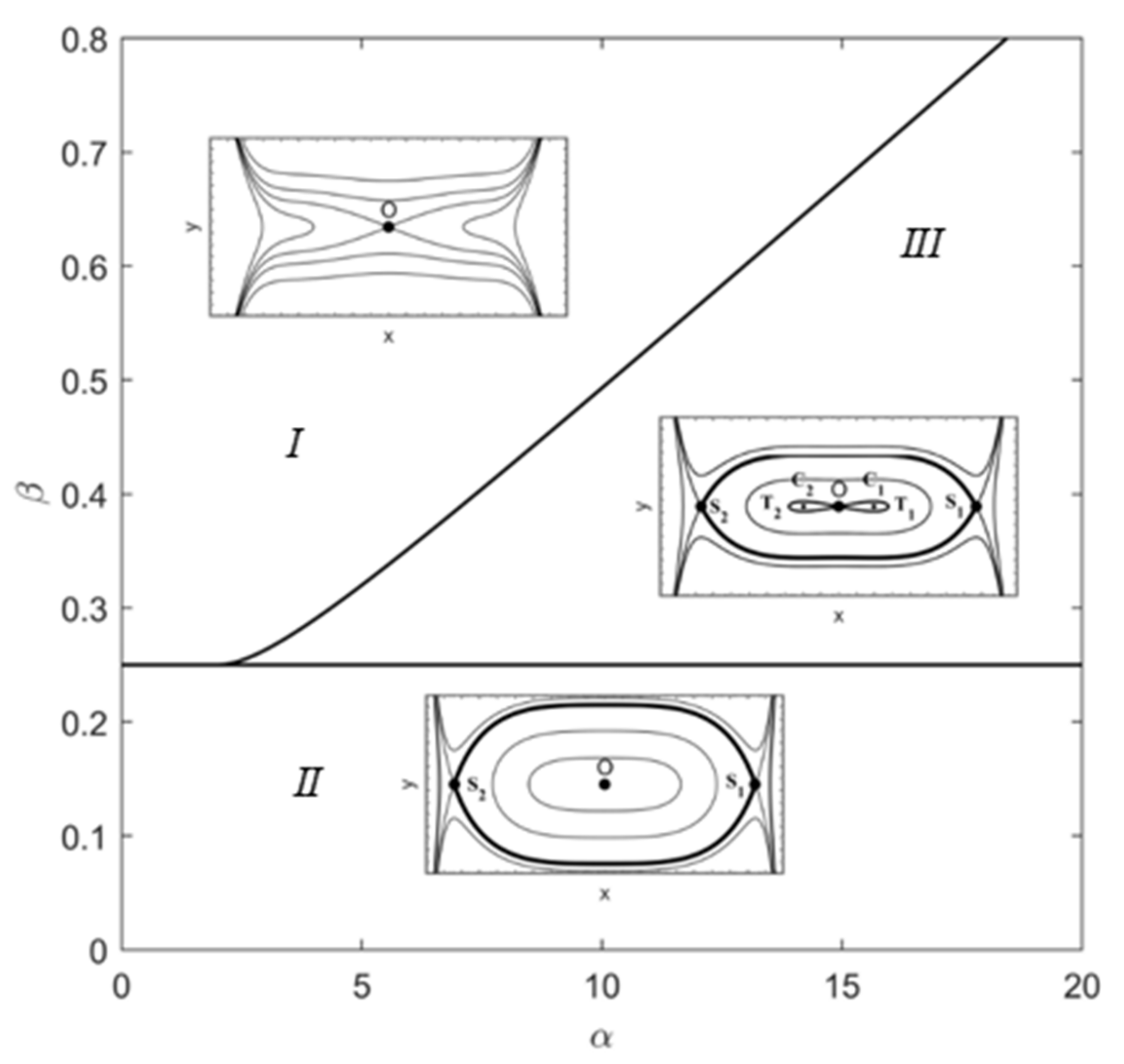
According to Theorems 1–3, the parameter plane α-β can be separated into three regions I, II and III, respectively, as depicted in Figure 2. With the help of the Hamilton function (7), the trajectories under different values of the parameters α and β are also classified, as shown in the following three cases.

Figure 2. Orbits of the unperturbed system (6) under different values of α and β.

Case 1: the values of α and β chosen in the region I. There will be one equilibrium and no potential well in the unperturbed system (6), meaning that each orbit will be unbounded for different values of the Hamiltonian $H\left(x,y\right)=E$. In this case, the phenomenon of pull in, namely static pull-in, will be unavoidable. Returning the conditions of the parameters α and β in Theorem 1 to the original system parameters, we can get the threshold of DC bias voltage for static pull-in

$$V_b>V_b{}^{Pull–in}=\max \{\sqrt{\frac{k_1{d}^3}{2A_0}},\hspace{1em}\frac{{(k_3{d}^2+m{\omega }_0^2)}^{\frac{3}{2}}}{3{\omega }_0{k}_3}\sqrt{\frac{2k_1}{3m{A}_{0}d}}\},$$

(18)

illustrating that the increase in DC bias voltage $V_b$ may lead to static pull-in [12]. Comparatively, the orbits in the other two regions are unnecessary to be unbounded, showing that for the parameter values in the regions II and III, pull in may be led by initial conditions rather than the system parameters. It is a so-called dynamic pull in [14,21].

Case 2: the values of the parameters α and β in the region II. There will be two saddle points crossing which there are heteroclinic orbits to surround a single potential well. Here the heteroclinic orbits are determined by $H\left(x,y\right)=H\left(x_s,0\right)$.

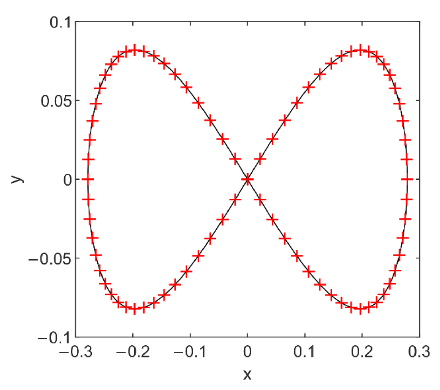
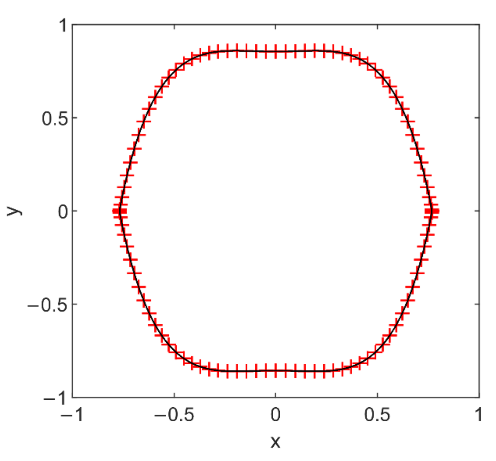
Case 3: the values of the parameters α and β in the region III. There will be two potential well centers $C_1(x_c,0)$ and $C_2(-x_c,0)$ surrounded by homoclinic orbits $H\left(x,y\right)=0$; outside of the homoclinic orbits, there are heteroclinic orbits determined by $H\left(x,y\right)=H\left(x_s,0\right)$ and crossing two saddle points $S_1(x_s,0)$ and $S_2(-x_s,0)$. Hence, the unperturbed system (6) contains homoclinic and heteroclinic orbits as well as multiple potential wells.

To discuss homoclinic bifurcation and heteroclinic bifurcation in the system, we focus on Case 3. Based on the same physical properties of the bilateral MEMS resonator in Refs. [8,19], in the following parts, some invariable parameters of the dimensionless system (5) can be calculated as:

$$\alpha =12,\hspace{1em}\beta =0.338,\hspace{1em}\mu =0.01,\hspace{1em}\omega =0.5.$$

(19)

The dimensionless AC-voltage amplitude $\gamma$ in the dimensionless system (5) will be changed to study the influence mechanism of dynamic response characteristics.

3. Global Bifurcations and Complex Dynamics

Since the dimensionless system (5) is a time-periodic perturbation of a Hamiltonian system, we may use the Melnikov method [19,20] to describe how the heteroclinic/homoclinic orbits break up in the presence of the perturbation. To begin with, homoclinic and heteroclinic orbits should be expressed as explicit functions of the time variable T. Note that the unperturbed system (6) contains fractional functions. Thus, these orbits cannot be written as the explicit functions of T. To tackle this problem, we will introduce new variables to express both the orbits and the time variable T explicitly. Then by substituting the explicit functions of new variables into the Melnikov functions, we can employ the Melnikov method smoothly.

3.1. Homoclinic Bifurcation Behavior

According to the Hamiltonian $H\left(x,y\right)=0$, the coordinates $x_{homo}$ and $y_{homo}$ of homoclinic orbits of the system (6) satisfy

$$y_{homo}=x_{homo}\sqrt{\frac{4\beta }{1-x_{homo}^2}-1-\frac{\alpha }{2}{x}_{homo}^2}$$

(20)

The intersection points between the orbits and the x axis are expressed as $T_1(x_e,0)$ and $T_2(-x_e,0)$ (see Figure 2), thus satisfying

$$x_e=\sqrt{\frac{\alpha -2-{\eta }_1}{2\alpha }}$$

(21)

where ${\eta }_1=\sqrt{{(\alpha +2)}^2-32\alpha \beta }$. By introducing a new time transformation $\phi (T)$ of the form [24]

$$\frac{d\phi (T)}{dT}=\mathrm{\Phi }(\phi )=\mathrm{\Phi }(\phi +2\pi ),$$

(22)

we assume at the saddle point O(0, 0) that

$$\phi (\infty )=\pi ,\hspace{1em}\phi (-\infty )=0.$$

(23)

It follows from Equations (20)–(23), the homoclinic orbits can be expressed by $\phi$ as

$$x_{homo}(\phi )=x_e\sin \phi ,\hspace{1em}{y}_{homo}=x_e^2\sin \phi \cos \phi \sqrt{\frac{{\eta }_1-\alpha x_e^2{\sin }^2\phi }{2(1-x_e^2{\sin }^2\phi )}}.$$

(24)

As shown in Figure 3, homoclinic orbits expressed by Equation (20) and the explicit functions of $\phi$ are in complete agreement with each other, which shows the validity of the explicit functions. Also, we have

$$T=\frac{\sqrt{2}\mathrm{sign}(\cos \phi )}{\sqrt{\alpha }{x}_e{}^2{x}_0}(E_1({\varphi }_1,\frac{{\eta }_1}{\alpha x_0})+E_3(\frac{x_0{\eta }_1}{\alpha x_e{}^2},{\varphi }_1,\frac{{\eta }_1}{\alpha x_0}))$$

(25)

in which $x_0=\sqrt{1-x_e^2}$ and ${\varphi }_1=-\mathrm{arcsinh}(\frac{\alpha x_e{}^4\left|\cos \phi \right|}{\sqrt{2(4+\alpha x_e{}^2)}})$; the functions $E_1$ and $E_3$ are the elliptic integrals of the first kind and the third kind, respectively.

Figure 3. Comparison of homoclinic orbits of the system (6) where the solid curve represents the exact model based on Hamiltonian and the sign + shows the orbits in explicit functions of $\phi$.

As well known, the Melnikov function [25,26,27,28] is a signed measure of the distance between the stable and un-stable manifolds for a perturbed system. If there are simple zeros in it, there will be intersection of homoclinic/heteroclinic orbits, corresponding to homoclinic/heteroclinic bifurcation. Assuming small parameters $\mu$ and $\gamma$ of the dimensionless system (5) as $\mu =\epsilon \tilde{\mu },\hspace{1em}\gamma =\epsilon \tilde{\gamma }$, and neglecting second-order terms of $\epsilon$ in Equation (5) yield

$$\ddot{x}+x+\alpha x^3+\frac{\beta }{{\left(1+x\right)}^2}-\frac{\beta }{{\left(1-x\right)}^2}=-\epsilon \tilde{\mu }\dot{x}+\frac{2\epsilon \beta \tilde{\gamma }\sin (\omega T)}{{\left(1-x\right)}^2}.$$

(26)

By substituting Equations (24) and (25) into the corresponding Melnikov function of the system (26), and returning the parameters into $\tilde{\mu }$ and $\tilde{\gamma }$ to $\mu$ and $\gamma$, respectively, we have

$$M_{homo}\left(T_0\right)=-\mu I_1+2\beta \gamma x_e\cos \left(\omega T_0\right)I_2+2\beta \gamma x_e\sin \left(\omega T_0\right)I_3.$$

(27)

where

$$\begin{array}{l}{I}_1=\sqrt{\alpha }{x}_e^3{\displaystyle {\mathrm{\int }}_{-1}^1{x}^2\sqrt{\frac{(3{\eta }_1-\alpha +2)+(\alpha -2-{\eta }_1)x^2}{(\alpha +2+{\eta }_1)+(\alpha -2-{\eta }_1)x^2}}dx}\\ =(\frac{(2+\alpha x_e{}^2)x_0\sqrt{2{\eta }_1}}{24\alpha }-\frac{4}{x_e{}^4})E_2(\mathrm{arccsch}(\frac{x_0}{x_e}),-\frac{\alpha x_0{}^2}{{\eta }_1})-\frac{4x_0}{x_e{}^3\sqrt{1-2x_e{}^2}}+\frac{4}{x_e{}^2}{E}_1(\mathrm{arccsch}(\frac{x_0}{x_e}),-\frac{\alpha x_0{}^2}{{\eta }_1})>0,\\ I_2={\displaystyle {\mathrm{\int }}_0^{\pi }\frac{\cos \phi \sin (\omega T(\phi ))}{{(1-x_e\sin \phi )}^2}d\phi },\hspace{1em}{I}_3={\displaystyle {\mathrm{\int }}_0^{\pi }\frac{\cos \phi \cos (\omega T(\phi ))}{{(1-x_e\sin \phi )}^2}d\phi };\end{array}$$

(28)

the functions $E_1$ and $E_2$ are the elliptic integrals of the first kind and the second kind, respectively. In Equation (28), the integrals $I_2$ and $I_3$ can be evaluated numerically [29]. If $2\beta \gamma x_e\sqrt{I_2{}^2+I_3{}^2}>\mu I_1$, namely,

$$V_{AC}>V_{AC}^{\mathrm{homo}0}=\frac{\mu V_{\mathrm{b}}{I}_1}{2\beta x_e\sqrt{I_2{}^2+I_3{}^2}}.$$

(29)

there will be a real number of $T_0$ satisfying $M_{homo}(T_0)=0$ and $M_{homo}{}^{\prime }(T_0)\ne 0$. It indicates that the equilibria of Equation $M_{homo}(T_0)=0$ are simple, enabling the existence of the transverse homoclinic orbits, i.e., homoclinic bifurcation. As homoclinic bifurcation usually triggers transient chaos [18,19,20], it follows from Equation (29) that the increase in AC voltage amplitude may induce transient chaos. Here, it can be calculated that $V_{AC}^{\mathrm{homo}0}=0.15 \mathrm{V}$.

In order to verify the accuracy of the theoretical prediction, we numerically simulate the solutions of Equation (5). In this paper, we utilize the fourth-order Runge-Kutta approach via MATLAB. For the ordinary differential Equation (5), the software package ODE45 is applied. Poincaré map [30], a commonly used method for investigating continuous time nonlinear systems, is employed to display the bifurcation process and rich dynamic behaviors. By setting ω = 0.5 and initial conditions $x(0)=0$ and $\dot{x}(0)=0$, the bifurcation diagram for the system (5) with the increase in AC voltage amplitude $V_{AC}$ is shown in Figure 4. Here, the points on the Poincaré map are collected from a cross-section at y = 0 in the sufficiently long time interval $5000\le T\le 7000$. As can be observed in Figure 4, there are periodic doubling windows and chaotic windows, implying that the MEMS resonator will undergo complex dynamics as $V_{AC}$ grows. Note that when $V_{AC}$ is higher than the threshold $V_{AC}^{\mathrm{homo}0}=0.15\mathrm{V}$ (see the red dashing line in Figure 4), chaos occurs. For instance, when $V_{AC}$ = 0.16 V, the phase portrait and the Poincaré map in Figure 5 depict the chaotic motion clearly. The numerical results closely match the analytical prediction of Equation (29), showing the validity of the analysis. It follows that the increase in $V_{AC}$ can induce homoclinic bifurcation, thus triggering chaos of the bilateral MEMS resonator.

Figure 4. Bifurcation diagram of the dimensionless system (5) when ω = 0.5.

Figure 5. Dynamic behavior of the system (5) for $V_{AC}=0.16 \mathrm{V}, V_{\mathrm{b}}=3.8 \mathrm{V}, \omega =0.5$: (a) phase portrait; (b) Poincáre map.

3.2. Heteroclinic Bifurcation Behavior

Similarly, we introduce a new variable $\psi$ to express the heteroclinic orbits of the unperturbed system (6) that satisfies

$$\frac{d\psi }{dT}=\mathrm{\Psi }(\psi )=\mathrm{\Psi }(\psi +2\pi ).$$

(30)

The heteroclinic orbits crossing the saddle points $S_1(x_s,0)$ and $S_2(-x_s,0)$ can be set as $x_0\left(\psi \right)=\pm x_s\cos \psi$ [24]. Here $x_s$ as the horizontal coordinate of a saddle point of the unperturbed system (6) can be solved from the following equation

$$4\beta =(1+\alpha x_s^2){(1-x_s^2)}^2.$$

(31)

Based on Equations (7) and (31), the coordinates $x_{hetero}$ and $y_{hetero}$ of the heteroclinic orbits can be expressed as

$$x_{hetero}(\psi )=\pm x_s\cos \psi ,\hspace{1em}{y}_{hetero}(\psi )=\mp x_s^2{\sin }^2\psi \sqrt{\frac{{\eta }_2+\alpha x_s{}^2{\cos }^2\psi }{2(1-x_s{}^2{\cos }^2\psi )}}.$$

(32)

where ${\eta }_2=2\alpha x_s^2-\alpha +2$. And the time variable T can be expressed by $\psi$ as

$$T=-\sqrt{\frac{2}{{\eta }_2}}\mathrm{sign}\left(\cos \psi \right)(E_1({\psi }_1,\frac{\alpha }{{\eta }_2})+\frac{1-x_s^2}{x_s^2}{E}_3(\frac{1}{x_s{}^2},{\psi }_1,\frac{\alpha }{{\eta }_2}))$$

(33)

where ${\psi }_1=\arcsin \left(x_s\left|\cos \psi \right|\right)$. The comparison of the orbits in both implicit functions $H\left(x,y\right)=H\left(x_s,0\right)$ and the explicit form (32) are presented in Figure 6. The complete agreement between them shows that the expression of heteroclinic orbits expressed by explicit functions of $\psi$ is accurate. Then, substituting heteroclinic orbits (32) and Equation (32) into the Melnikov function of the approximate system (26) yields

$$M_{hetero}(t_0)=-2\mu J_1\mp 2\beta \gamma x_s\sin \left(\omega T_0\right)J_2\mp 2\beta \gamma x_s\cos \left(\omega T_0\right)J_3,$$

(34)

where

$$\begin{array}{l}{J}_1={\displaystyle {\mathrm{\int }}_0^{\frac{\mathsf{\pi }}{2}}{\sin }^3\phi \sqrt{\frac{2\beta (2x_s^2-1+x_s{}^2{\cos }^2\phi )}{{(1-x_s{}^2)}^2\left(1-x_s{}^2{\cos }^2\phi \right)}+\frac{1}{2}}}d\phi \\ =\frac{x_s}{3}\sqrt{\frac{({\eta }_2+\alpha x_s^2)(1-x_s^2)}{2}}-\frac{2+\alpha {(1-x_s^2)}^2}{6\alpha {(1-x_s^2)}^2}\sqrt{2{\eta }_2}{E}_2\left(\arcsin x_s,\frac{\alpha }{{\eta }_2}\right)+\frac{(1+\alpha x_s^2)(1-x_s^2)}{3\alpha x_s{}^2}\sqrt{2{\eta }_2}{E}_1\left(\arcsin x_s,\frac{\alpha }{{\eta }_2}\right)>0,\\ J_2={\displaystyle {\mathrm{\int }}_0^{\mathsf{\pi }}\frac{\sin \psi \cos \left(\omega T\left(\psi \right)\right)}{{\left(1-x_s\cos \psi \right)}^2}d\psi },J_3={\displaystyle {\mathrm{\int }}_0^{\mathsf{\pi }}\frac{\sin \psi \sin \left(\omega T\left(\psi \right)\right)}{{\left(1-x_s\cos \psi \right)}^2}}d\psi .\end{array}$$

(35)

Figure 6. Comparison of heteroclinic orbits of the system (6) where the solid curve represents the exact model based on Hamiltonian and the sign + shows the orbits in explicit functions of $\psi$.

When $\beta \gamma x_s\sqrt{J_2^2+J_3^2}\ge \mu J_1$, i.e.,

$$V_{AC}>V_{AC}^{Hetero0}=\frac{\mu V_{\mathrm{b}}{J}_1}{\beta x_s\sqrt{J_2{}^2+J_3{}^2}}.$$

(36)

there will be a simple equilibrium of the Melnikov function (34), enabling the existence of the transverse heteroclinic orbits, and the dimensionless system (5) may undergo a type of initial-sensitive motion. Here, it can be calculated that $V_{AC}^{hetero0}=0.25 \mathrm{V}$, much higher than the threshold for homoclinic-bifurcation chaos $V_{AC}^{homo0}=0.15 \mathrm{V}$ (see last section), indicating that complex dynamic behavior induced by heteroclinic bifurcation will be different from chaos. Since heteroclinic bifurcation in nonlinear systems is usually the mechanism responsible for triggering fractal erosion of safe basin [13,21,31], for $V_{AC}$ higher than the threshold $V_{AC}^{hetero0}$, erosion of safe basin of the dimensionless system (5) will be expected. In Equation (5), the escape solution x = 1 or −1 means pull in to the upper electrode or the lower one, respectively. All the initial conditions leading to pull in construct the basin of attraction of pull-in attractors, which can be considered as dangerous basin [21]. In contrast, for bounded solutions satisfying $\left|x(T)\right|<1$, the union of their basins of attraction is defined as safe basin. The intermingle of safe basin and dangerous basin implies that a subtle disturbance of initial conditions may change the dynamics of the system (5), for instance, from a bounded motion to pull in. it can intuitively depict the phenomenon pull-in instability.

In order to verify the criterion obtained in this section, numerical simulations are carried out. The 4th Runge-Kutta approach and the point-mapping method [22,23] are employed to describe safe basin. In this paper, safe basin is drawn in the sufficiently large space region defined as −1.2 ≤ x(0) ≤ 1.2, −1.0 ≤ y(0) ≤ 1.0 by generating a 200 × 200 array of initial conditions for each of those starting points. The escaping set for infinite time is approximated with good accuracy by a study of 1000 excited circles. The time step is taken as 0.01. The white region represents the numerical approximation to basin of pull-in attractors, and the black region is safe basin.

The variation of safe basin with the increase in $V_{AC}$ is given in Figure 7. It can be noticed that when there is no AC voltage in the vibrating system (see Figure 7a), the boundary of safe basin is nearly the same as the region surrounded by heteroclinic orbits. When $V_{AC}$ increases to 0.15 V (see Figure 7b), namely the threshold for homoclinic bifurcation, safe basin becomes smaller, but its boundary is still smooth. When $V_{AC}$ reaches 0.3 V (see Figure 7c), higher than the threshold $V_{AC}^{hetero0}$, the fractal fingers occur on the basin boundary, which is in agreement with our theoretical prediction. As $V_{AC}$ continue to increase, the fractality of safe basin becomes more and more visible (see Figure 7d,e). Finally, when $V_{AC}$ grows to 1.05 V, the whole initial-condition plane is eroded to be white (see Figure 7f), meaning that pull in of the MEMS resonator is unavoidable, i.e., static pull-in. It shows that in the dynamic system of the bilateral MEMS resonator, heteroclinic bifurcation induces pull-in instability.

Figure 7. Safe basins of the system (5) under different values of AC voltage amplitude: (a) $V_{AC}=0 \mathrm{V}$; (b) $V_{AC}=0.15 \mathrm{V}$; (c) $V_{AC}=0.30 \mathrm{V}$; (d) $V_{AC}=0.50 \mathrm{V}$; (e) $V_{AC}=0.70 \mathrm{V}$; (f) $V_{AC}=1.05 \mathrm{V}$.

4. Control of Complex Dynamics via Delayed Feedback

In this section, two types of linear-delayed feedback controllers, i.e., delayed-position feedback and delayed-velocity feedback, are applied on the DC voltage source to stabilize the micro resonator. The corresponding control diagram is schemed in Figure 8 where w represents the position $z(t)$ or the velocity $\frac{dz}{dt}$. The governing controlled system can be expressed as

$$m\frac{{\mathrm{d}}^{2}z}{\mathrm{d}{t}^2}+c\frac{\mathrm{dz}}{\mathrm{d}t}+k_{1}z+k_3{z}^3=\frac{A_0}{2{(d-z)}^2}{(V_b+G(w(t-\tilde{\tau })-w)+V_{AC}\sin \mathrm{\Omega }t)}^2-\frac{A_0}{2{(d+z)}^2}{(V_b+G(w(t-\tilde{\tau })-w))}^2,$$

(37)

where $\tilde{\tau }$ is time delay, and G the gain of the feedback controller. G and $\tilde{\tau }$ are independent parameters. When $\tilde{\tau }$ = 0, the controlled term becomes that $G(w(t-\tau )-w(t))=0$, and then the controlled system becomes the original system (1). Setting

$$g_p=\frac{Gd}{V_b},\hspace{1em}{g}_v=\frac{{\omega }_{0}Gd}{V_b},\hspace{1em}\tau ={\omega }_0\tilde{\tau },$$

(38)

and substituting Equation (4) into the controlled system (37), we will have

$$\ddot{x}+\mu \dot{x}+x+\alpha x^3=\frac{\beta }{{(1-x)}^2}{(1+g_p(x(T-\tau )-x)+\gamma \sin \omega T)}^2-\frac{\beta }{{(1+x)}^2}{(1+g_p(x(T-\tau )-x))}^2,$$

(39)

for $w(t)=x(t)$, and

$$\ddot{x}+\mu \dot{x}+x+\alpha x^3=\frac{\beta }{{(1-x)}^2}{(1+g_v(\dot{x}(T-\tau )-\dot{x})+\gamma \sin \omega T)}^2-\frac{\beta }{{(1+x)}^2}{(1+g_v(\dot{x}(T-\tau )-\dot{x}))}^2,$$

(40)

for $w(t)=\frac{dx(t)}{dt}$. Considering the engineering application, we do not discuss the periodic characteristics of the dimensionless time delay $\tau$ but restrict that $0\le \tau <2\pi$. Since there is no signal that can be returned to the delayed-feedback control system (37) before $t=0$, the initial conditions for the controlled system can be supposed as $x(t)=0$ and $x^{\prime }(t)=0$ for $-\tau \le t<0$ [23,32]. Then the initial-condition space of the delayed system can be projected onto the initial-phase plane $x(0)-x^{\prime }(0)$. It means that we can set $x(T)=y(T)=0$ for $-\tau \le t<0$ in the dimensionless controlled systems (39) and (40), and still depict safe basin in the initial-state plane $x(0)-y(0)$, the same as the original system (5). To be different from Section 3, the software package applied in this section is DDE23, as the controlled systems (39) and (40) are delayed differential equations rather than ordinary differential ones.

Figure 8. Schematic diagram of the delayed-feedback-control bilateral MEMS resonator.

4.1. Delayed Position Feedback

To study the control mechanism of chaos and pull-in instability in the delayed system via the Melnikov method conveniently, the precondition is that the delayed-position feedback $g_p(x(T-\tau )-x)$ can be treated as a perturbed term of the controlled system (39). In other words, we should ensure that the value of time delay τ will not exceed the first stability switch of equilibria in a linearized system [23,32]. In this situation, we can expand the delayed feedback of the system (39) into Taylor’s series so as to obtain an approximately ordinary different equation. On this basis, similar to the last section, the Melnikov method can be applied to discuss critical conditions for chaos and pull-in instability.

Since $\mu >0$ and $\alpha -2-3\alpha x_c{}^2>0$, in the linearized system of the uncontrolled system (5), the two equilibria $C_1(x_c,0)$ and $C_2(-x_c,0)$ are stable. Thus, we should present the linear-stability analysis in the vicinity of the two equilibria. The position $x$ is set as

$$x=\pm x_c+\epsilon u+O({\epsilon }^2),$$

(41)

where $u=\mathrm{O}\left(1\right)$. Substituting (41) into the delayed system (39), expanding the terms $\frac{\beta }{{(1-x)}^2}$ and $\frac{\beta }{{(1+x)}^2}$ in Taylor’s series and neglecting $\epsilon$ terms and higher-order terms of $\epsilon$ yield, the following delayed-linear system

$$\ddot{u}+\mu \dot{u}=\frac{2x_c{}^2(2-\alpha +3\alpha x_c{}^2)}{1-x_c{}^2}u+2(1+\alpha x_c{}^2)x_c{g}_p(u(T-\tau )-u)$$

(42)

Its characteristic equation can be written by

$${\lambda }^2+\mu \lambda +\rho -2x_c(1+\alpha x_c{}^2)g_p(e^{-\lambda \tau }-1)=0$$

(43)

where $\rho =\frac{2x_c{}^2(\alpha -2-3\alpha x_c{}^2)}{1-x_c{}^2}>0.$ Substituting $\lambda =iv$ into Equation (43), separating the imaginary and real parts, and eliminating the triangular functions yield

$$v^4+v^2(-2\rho -4x_c(1+\alpha x_c{}^2)g_p+{\mu }^2)+\rho (\rho +4x_c(1+\alpha x_c{}^2)g_p)=0$$

(44)

According to Equation (44), if the gain $g_p$ satisfies

$$4x_c(1+\alpha x_c{}^2)g_p>{\mu }^2+2\mu \sqrt{\rho },$$

(45)

there will be two different positive solutions of Equation (44) expressed as $v_{+}$ and $v_{-}$. And the critical value of time delay for the stability switch of the two equilibria $C_1(x_c,0)$ and $C_2(-x_c,0)$ can be expressed as

$${\tau }_{+}(0)=\frac{1}{v_{+}}(2\pi -\arccos (1+\frac{\rho -v_{+}{}^2}{2x_c(1+\alpha x_c{}^2)g_p}))$$

(46)

Thus, the delayed position feedback can be considered as the perturbed term when $0<\tau <{\tau }_{+}(0)$. Fixing $g_p=0.2$, it can be calculated from Equation (46) that ${\tau }_{+}(0)\approx 1.53$. When applying the delayed position feedback suppressing global bifurcation behaviors, it is better to ensure the delay $\tau$ less than ${\tau }_{+}(0)$.

4.1.1. Control of Chaos

In the delayed-position-feedback controlled system (39), for $0<\tau <{\tau }_{+}(0)$, rescaling that $\tau =\epsilon \widehat{\tau }$, expanding the delayed feedback $g_p(x(T-\tau )-x$ in Taylor’s series, neglecting ${\epsilon }^2$ terms and higher-order terms of $\epsilon$, and then returning to the non-dimensional variables, we can approximate Equation (39) as the following ordinary differential equation

$$\ddot{x}+x+\alpha x^3+\frac{\beta }{{(1+x)}^2}-\frac{\beta }{{(1-x)}^2}=-\mu \dot{x}+\frac{2\beta \gamma \sin \omega T}{{(1-x)}^2}-\frac{8\beta g_p\tau x\dot{x}}{{(1-x^2)}^2}$$

(47)

The similar as the uncontrolled system (5), based on homoclinic orbits (24) and Equation (25), the Melnikov function of the system (47) can be written as

$$M_{homo-P}(t_0)=-\mu I_1\pm 2\beta \gamma (I_2\cos (\omega T_0)+I_3\sin (\omega T_0)-\beta g_p\tau I_p$$

(48)

where

$$I_p=\frac{{(\alpha -2-{\eta }_1)}^2\sqrt{{\eta }_1}}{2\sqrt{2}{\alpha }^2}{\displaystyle {\mathrm{\int }}_0^{\pi }{\sin }^{2}2\phi \sqrt{\frac{1-\frac{\alpha -2-{\eta }_1}{2{\eta }_1}{\sin }^2\phi }{{(1-\frac{\alpha -2-{\eta }_1}{2\alpha }{\sin }^2\phi )}^5}}d\phi }>0$$

(49)

The integral $I_p$ in the above equation can be evaluated numerically.

When $2\beta \gamma \sqrt{I_2{}^2+I_3{}^2}>\mu I_1+\beta g_p\tau I_p$, namely

$$V_{AC}>V_{AC}^{Homo-P}=V_{AC}^{Homo0}+\frac{g_p\tau V_b{I}_p}{2\sqrt{I_2{}^2+I_3{}^2}}.$$

(50)

there will be a simple zero in the Melnikov function. Accordingly, the threshold of $V_{AC}$ for homoclinic bifurcation of the system is $V_{AC}^{Homo-P}$ of the above equation. It follows from Equation (50) that for $g_p>0$, the threshold of $V_{AC}$ for homoclinic bifurcation in the delayed-position-feedback controlled system will become higher than in the uncontrolled system. It illustrates the mechanism of delayed-position feedback on controlling chaos.

Given $g_p=0.2$, the change of $V_{AC}$ threshold with the increase in the delay τ is depicted in Figure 9. Here τ ranges from 0 to 0.25, satisfying τ<<${\tau }_{+}(0)$. The numerical results of $V_{AC}^{Homo-P}$ are obtained under which the transient chaos occurs. Each numerical value of $V_{AC}^{Homo-P}$ has two decimal places. In Figure 9, the numerical results for $V_{AC}^{Homo-P}$ are in substantial agreement with the analytical ones. It demonstrates that the threshold of AC voltage amplitude for transient chaos increases monotonically with the delay τ for a positive gain and a small τ. 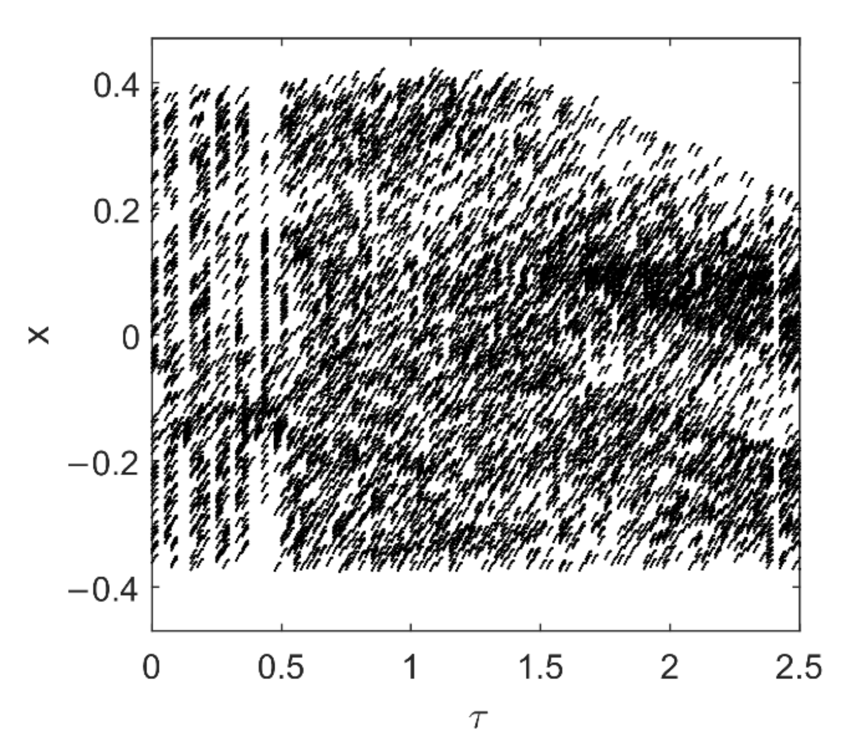For example, setting $V_{AC}$ = 0.16 V, one can observe the evolution of dynamics with time delay in Figure 10. As shown in the bifurcation diagram of Figure 10a, with the increase in time delay, the transient chaos is reduced effectively. For example, when τ = 0.13, it becomes a periodic attractor (see Figure 10b). It shows that the delayed position feedback can be used to suppress chaos of the micro resonator effectively.

Figure 9. Variation of $V_{AC}$ threshold for homoclinic bifurcation with $\tau$ when $g_p=0.2$.

Figure 10. Dynamic behavior of the delayed system (39) when $g_p=0.2$ and $V_{AC}=0.16 \mathrm{V}$ (a) Bifurcation with τ in Poincáre map (b) Phase map when τ = 0.12.

4.1.2. Control of Pull-In Instability

Similar to last section, we can also employ the Melnikov method to obtain the critical condition for heteroclinic bifurcation of the controlled system (47). Substituting heteroclinic orbits (31) and Equation (32) into the Melnikov function of Equation (47) yields

$$M_{hetero-P}(T_0)=-2\mu x_s{}^2{J}_1\mp 2\beta \gamma x_s(J_2\sin (\omega T_0)+J_3\cos (\omega T_0))-8\sqrt{2\beta }{x}_s\tau g_p{J}_p,$$

(51)

where

$$J_p=\frac{\sqrt{\alpha x_s^2+{\eta }_2}(x_s^2+3x_s{}^2\beta +\beta -1)-\sqrt{{\eta }_2}(x_s^2+3x_s{}^2\beta +3\beta -1)}{3{(1-x_s^2)}^{\frac{3}{2}}}+\sqrt{\alpha }\beta (\arcsin h\frac{2\sqrt{\alpha }{x}_s}{\sqrt{1+\alpha x_s^2}}-\arcsin h\frac{\sqrt{2\alpha }{x}_s}{\sqrt{1+\alpha x_s^2}})>0.$$

(52)

For $\beta \gamma \sqrt{J_2^2+J_3^2}>\mu x_s{J}_1+4\sqrt{2\beta }{g}_p\tau J_p$, namely

$$V_{AC}>V_{AC}^{Hetero-P}=V_{AC}^{Hetero0}+\frac{4\sqrt{2}{g}_p\tau V_{\mathrm{b}}{J}_p}{\sqrt{\beta (J_2^2+J_3^2)}}$$

(53)

according to the global bifurcation theory [25,26,27,28], there will be a simple equilibrium of the above Melnikov function, implying heteroclinic bifurcation. It shows in Equation (53) that the increase in $V_{AC}$ in the delayed-position-feedback controlled system can also trigger heteroclinic bifurcation, similar as in the uncontrolled system. For $g_p>0$, one has $V_{AC}^{Hetero-P}>V_{AC}^{Hetero0}$, showing that for a positive gain, heteroclinic bifurcation will occur under a higher AC voltage amplitude in the controlled system than in the uncontrolled system. It shows the control mechanism of heteroclinic-bifurcation behavior.

In light of the theoretical predictions, we present numerical examples to verify their validity. As shown in Figure 11, the theoretical results for $V_{AC}^{Hetero-P}$ increase monopoly with the dimensionless delay τ for $g_p=0.2$. The numerical values of $V_{AC}^{Hetero-P}$ are obtained at the point which the boundary of safe basin begins to be unsmooth. In other words, if $V_{AC}$ is less than the numerical results of $V_{AC}^{Hetero-P}$, the boundary of safe basin will still be smooth. It can be seen in Figure 11 that the numerical results match the theoretical ones well, which illustrates that under a positive gain, the delayed position feedback can be used to control pull-in instability.

Figure 11. Variation of $V_{AC}$ threshold for heteroclinic bifurcation with τ for $g_p=0.2$.

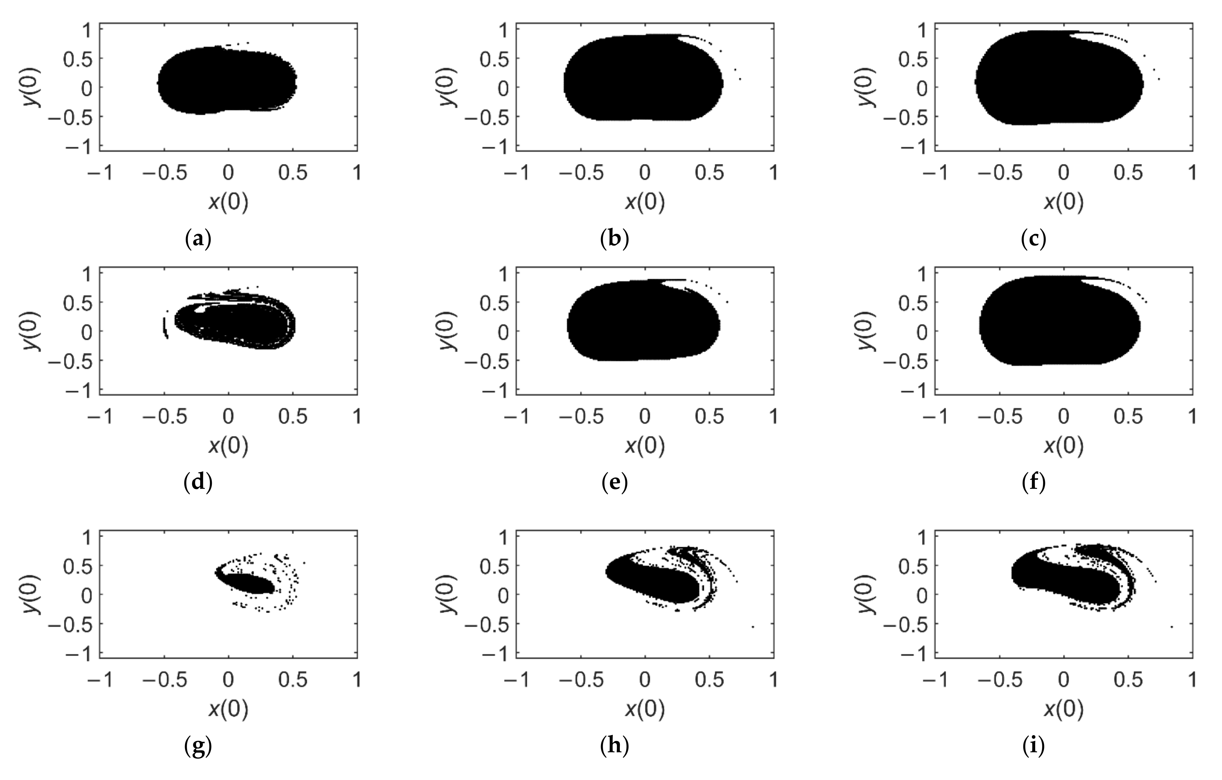
To depict the effect of delayed position feedback on controlling pull-in instability in details, the evolution of safe basin with the increase in τ is presented in Figure 12 where the delay is short, satisfying $\tau <<{\tau }_{+}(0)$. When τ = 0 (see Figure 12a,d,g), safe basins mean those of the uncontrolled system, which contain fractal boundaries, illustrating pull-in instability. With the increase in the delay τ, the fractal extent, namely the probability of pull-in instability, is obviously lessened, and the basin area enlarged, which can be observed in each line of Figure 12. When $\tau =0.55$, the basin boundary under $V_{AC}=0.46 \mathrm{V}$ becomes smooth (see Figure 12b), and the other two basins are enlarged whose boundaries are still fractal (see Figure 12e,h). When $\tau =0.81$, the basin boundary under $V_{AC}=0.52 \mathrm{V}$ becomes smooth too (see Figure 12f). Even though safe basin in Figure 12i still has a fractal boundary, the situation is much better than in the uncontrolled system: at least the vicinity of the origin is black, showing that dynamic pull-in will not occur in the initial-condition region.

Figure 12. Safe basins of the controlled system (39) under different values of $V_{AC}$ and τ: (a) $V_{AC}=0.46 \mathrm{V},\hspace{1em}\tau =0$; (b) $V_{AC}=0.46 \mathrm{V},\hspace{1em}\tau =0.55$; (c) $V_{AC}=0.46 \mathrm{V},\hspace{1em}\tau =0.75$; (d) $V_{AC}=0.52 \mathrm{V},\hspace{1em}\tau =0$; (e) $V_{AC}=0.52 \mathrm{V},\hspace{1em}\tau =0.55$; (f) $V_{AC}=0.52 \mathrm{V},\hspace{1em}\tau =0.75$; (g) $V_{AC}=0.81 \mathrm{V},\hspace{1em}\tau =0$; (h) $V_{AC}=0.81 \mathrm{V},\hspace{1em}\tau =0.55$; (i) $V_{AC}=0.81 \mathrm{V},\hspace{1em}\tau =0.75$.

4.2. Delayed Velocity Feedback

Similar to delayed-position feedback, we also expect to treat the delayed velocity feedback as a perturbed term so as conveniently to discuss the global bifurcation of the controlled system. Thus, the value of time delay τ should be kept less than the first stability switch of equilibria in the linearized system. Based on the linearized system in the vicinity of the stable equilibria of the uncontrolled system (5) and the corresponding characteristic equation, the critical condition for the stability switch is that there exists a purely imaginary eigenvalue $\lambda =iv$ satisfying

$$-v+(\frac{1+3x_c^2\alpha }{v}-\frac{4\beta (1+3x_c^2)}{v{(1-x_c^2)}^2})=\frac{8\beta g_v{x}_c}{{(1-x_c^2)}^2}\sin v\tau ,\hspace{1em}\mu +\frac{8\beta x_c{g}_v}{{(1-x_c^2)}^2}=\frac{8\beta g_v{x}_c}{{(1-x_c^2)}^2}\cos v\tau$$

(54)

For a positive gain $g_v$, since $\mu >0$, it is easy to conclude that there is no real root of $v$ in Equation (54). It implies that the stability of the two equilibria will not be changed by the delayed velocity feedback under a positive $g_v$.

4.2.1. Suppression of Chaos

Now expressing a short time delay $\tau$ as $\epsilon \tilde{\tau }$, expanding $g_v(\dot{x}(T-\tau )-\dot{x})$ in Taylor’s series, neglecting higher-order terms of $\epsilon$, and returning the parameters to the non-dimensional parameters, we approximate the delayed-velocity-feedback controlled system as

$$\ddot{x}+x+\alpha x^3+\frac{\beta }{{(1+x)}^2}-\frac{\beta }{{(1-x)}^2}=-\mu \dot{x}+\frac{2\beta \gamma \sin \omega T}{{(1-x)}^2}-\frac{8\beta g_v\tau x\ddot{x}}{{(1-x^2)}^2}$$

(55)

Substituting homoclinic orbits (24) and Equation (25) into the Melnikov function of the above ordinary differential-equation yields

$$M_{homo-V}(T_0)=-\mu I_1\pm 2\beta \gamma (I_2\cos (\omega T_0)+I_3\sin (\omega T_0)-2g_v\tau \beta {\displaystyle {\int }_{-\infty }^{+\infty }(\frac{1}{{(1-x_{homo})}^2}-\frac{1}{{(1+x_{homo})}^2})}{y}_{homo}d{y}_{homo}(\phi )$$

(56)

Since ${\displaystyle {\mathrm{\int }}_{-\infty }^{+\infty }(\frac{1}{{(1-x_{homo})}^2}-\frac{1}{{(1+x_{homo})}^2})}{y}_{homo}d{y}_{homo}(\phi )=0$, one has $M_{homo-V}(T_0)=M_{homo}(T_0)$. Accordingly, $V_{AC}^{Homo-V}=V_{AC}^{Homo0}$. It indicates that the delayed velocity feedback cannot work for reducing transient chaos. It can also be verified by the numerical bifurcation diagram in Figure 13 for $g_v$ = 0.2. As depicted in Figure 13, with the variation of the delay $\tau$, the dynamic behavior is still complex.

Figure 13. Bifurcation of the delayed-velocity-feedback controlled system (40) with $\tau$ in Poincaré map for $g_v=0.2$ and $V_{AC}=0.16 \mathrm{V}$.

4.2.2. Suppression of Pull-In Instability

Similarly, by substituting heteroclinic orbits (31) and Equation (32) into the Melnikov function of Equation (55), we can the Melnikov function as follows

$$M_{hetero-V}(T_0)=-2\mu J_1\mp 2\beta \gamma x_s\sin \left(\omega T_0\right)J_2\mp 2\beta \gamma x_s\cos \left(\omega T_0\right)J_3-8\beta g_v\tau J_v$$

(57)

where

$$J_v=\frac{3}{x_s^3}-\frac{\beta \left(72-51x_s^2-8x_s^4+3x_s^6\right)}{6x_s^3{(1-x_s^2)}^{\frac{3}{2}}}+\frac{\left(4+\beta -6\alpha +6\alpha x_s^2\right)}{2x_s^2}\mathrm{arctanh}\left(x_s\right)>0$$

(58)

According to the theory of global bifurcation, the critical condition for heteroclinic bifurcation is $\beta \gamma x_s\sqrt{J_2^2+J_3^2}>\mu J_1+4\beta g_v\tau J_v$. Expressing it by the original parameters $V_{AC}$ and $V_{\mathrm{b}}$ yields

$$V_{AC}>V_{AC}^{Hetero-V}=V_{AC}^{Hetero0}+\frac{4g_v\tau V_{\mathrm{b}}{J}_v}{x_s\sqrt{J_2{}^2+J_3{}^2}}.$$

(59)

In Equation (59), $V_{AC}^{Hetero-V}$ means the threshold of AC voltage amplitude for pull-in instability in the delayed-velocity-feedback controlled system. It follows that $V_{AC}^{Hetero-V}>V_{AC}^{Hetero0}$ for $g_v>0$, demonstrating that under a positive gain, the delayed velocity feedback can be useful to control heteroclinic bifurcation behavior.

The effectiveness of the delayed-velocity feedback control can be verified by the comparison of the theoretical thresholds and the numerical ones for pull-in instability in Figure 14 for $g_v=0.2$. Furthermore, the sequences of safe basin with the increase in time delay are depicted in detail (see Figure 15). It follows from the comparison of safe basins under the same values of $V_{AC}$ and different values of τ that under a positive gain $g_v$, the delayed-velocity feedback can restrict the extent of pull-in instability and dynamic pull in successfully (see each row of Figure 15). When τ = 0, the delayed system becomes the uncontrolled one; thus, for $V_{AC}$ higher than 0.25 V ($V_{AC}^{Hetero0}$), safe basin is fractal (see the first column of Figure 15), showing the occurrence of pull-in instability. With the increase in time delay τ, the fractal extent of safe basin will be reduced. When $\tau =1.6$, the basin boundary under $V_{AC}=0.46 \mathrm{V}$ turns smooth (see Figure 15b). When $\tau$ reaches 2.0, the basin boundary under $V_{AC}=0.52 \mathrm{V}$ also becomes smooth, as shown in Figure 15f. Comparing with the uncontrolled safe basin in Figure 15g, although safe basin in Figure 15i is still fractal, the vicinity of the point O(0, 0) and $C_1(x_c,0)$ becomes black, showing that in this region, the MEMS resonator under the delayed velocity feedback will not undergo pull-in, thus having a more stable performance.

Figure 14. Variation of AC voltage threshold for heteroclinic bifurcation with $\tau$ when g_v = 0.2.

Figure 15. Safe basins of velocity-feedback-controlled system (40) under different $V_{AC}$ and τ: (a) $V_{AC}=0.46 \mathrm{V},\hspace{1em}\tau =0$; (b) $V_{AC}=0.46 \mathrm{V},\hspace{1em}\tau =1.6$; (c) $V_{AC}=0.46 \mathrm{V},\hspace{1em}\tau =2$; (d) $V_{AC}=0.52 \mathrm{V},\hspace{1em}\tau =0$; (e) $V_{AC}=0.52 \mathrm{V},\hspace{1em}\tau =1.6$; (f) $V_{AC}=0.52 \mathrm{V},\hspace{1em}\tau =2$; (g) $V_{AC}=0.81 \mathrm{V},\hspace{1em}\tau =0$; (h) $V_{AC}=0.81 \mathrm{V},\hspace{1em}\tau =1.6$; (i) $V_{AC}=0.81\mathrm{V},\hspace{1em}\tau =2.0$.

5. Discussion

In the dynamic systems of MEMS resonators, initial-sensitive dynamic behaviors such as chaos and pull-in instability are unfavorable for causing the loss-of-performance reliability of these devices. It is known that initial-sensitive dynamic behaviors are usually attributed to global bifurcations. To understand their mechanisms adequately and to propose effective control strategies, we consider a typical bilateral MEMS resonator and discuss its global bifurcation behaviors analytically and numerically.

First, the ordinary differential equation governing the vibrating system of the MEMS resonator is made dimensionless. The static bifurcation of equilibria is investigated for the unperturbed system. The bifurcation sets of the equilibria in parameter space are constructed to demonstrate that the number and shapes of potential wells depend on DC bias voltage. The increase in DC bias voltage may lead to static pull-in of the micro resonator. In a certain range of DC bias voltage, the unperturbed system contains both homoclinic orbits and heteroclinic orbits, implying the possibility of rich complex dynamics.

Next, by fixing the physical parameters of the micro resonator and varying the AC voltage amplitude, the case of coexisting homoclinic orbits and heteroclinic ones is discussed in detail. The Melnikov method is employed to provide analytical critical conditions for global bifurcations. It is worth mentioning that this vibrating system contains fractional terms which constitute an obstacle for expressing the unperturbed orbits in explicit functions of time variable. Thus, the Melnikov method cannot be applied conveniently. To tackle this problem, new variables are introduced to express both the orbits and the time variable explicitly so as to detect the analytical criteria for global bifurcations via the Melnikov method.

Furthermore, the analytical results are verified by the numerical simulations in the form of phase maps, safe basins, bifurcation diagrams and Poincaré maps. Fractal erosion of safe basin is induced to depict pull-in instability intuitively. It is found that chaos and pull-in instability are different initial-sensitive phenomena attributed to homoclinic and heteroclinic bifurcation, respectively. The increase in AC voltage amplitude may trigger chaos and pull-in instability of this MEMS resonator successively.

Consequently, delayed-position feedback and delayed-velocity feedback are applied to the DC-voltage source to stabilize the micro resonator, respectively. To study the control mechanisms for chaos and pull-in instability in the delayed system conveniently, we treat the two types of delayed feedback as perturbed terms by expanding them in Taylor’s series so as to transform these delayed systems to ODEs. To this end, we discuss the first stability switch of equilibria in linearized controlled systems to make sure the delay is much less than the original system, thus it will not change the original stability of equilibria. On this basis, the similar as the original system, critical conditions for global bifurcation under control are discussed and confirmed by the numerical simulations. It shows that the two types of delayed feedback applied on DC bias voltage can both reduce pull-in instability effectively. The control mechanism behind is that under a positive gain coefficient, the AC voltage amplitude threshold of heteroclinic bifurcation increases with time delay. For suppressing chaos, only delayed-position feedback under a positive gain can be effective.

This work presents a detailed analysis of pull-in instability and chaos of a typically MEMS resonator as well as their control, which may provide some potential applications for the design and control of relevant MEMS devices. It should be pointed out that the results are limited to the fixed physical properties of this MEMS resonator. We have not yet discussed the effect of physical properties on triggering complex responses. For a better performance reliability of MEMS resonators, these should be taken into account in theoretical study as well as experiment, which will be included in our future work.