Dual Penta-Compound Combination Anti-Synchronization with Analysis and Application to a Novel Fractional Chaotic System

Abstract

This paper studies a fractional-order chaotic system with sine non-linearities and highlights its dynamics using the Lyapunov spectrum, bifurcation analysis, stagnation points, the solution of the system, the impact of the fractional order on the system, etc. The system considering uncertainties and disturbances was synchronized using dual penta-compound combination anti-synchronization among four master systems and twenty slave systems by non-linear control and the adaptive sliding mode technique. The estimates of the disturbances and uncertainties were also obtained using the sliding mode technique. The application of the achieved synchronization in secure communication is illustrated with the help of an example.

1. Introduction

The three-centuries-old theory of fractional calculus, which is the generalization of integer calculus, has found glory quite recently. Fractional calculus is being implemented to model various real-life systems in almost all disciplines. In fact, fractional calculus is seen as the future of mathematical modeling. Fractional calculus with its better hereditary properties is used to model various biological models such as the prey–predator model [1] and the human liver [2], engineering models such as harmonic oscillators [3] and thermostats [4], geophysical models such as Earth’s dynamo [5], and so on. Fractional computations have attracted researchers worldwide in dynamical systems such as the Chua circuit, the Duffing system, and the logistic system. Chaotic systems being highly sensitivity to system values have contributed greatly in the development of information security, computers, communications [6], and encryption [7]. Chaotic systems help mask the information signal to avoid hacking by intruders. Chaos synchronization plays a major role in the decryption of the information signal from the masked signal. Chaotic systems with their positive Lyapunov spectrum component resist their synchronization with other chaotic systems. Many standard and non-standard chaotic systems have been constructed recently. The chaotic systems are classified on the basis of the number of stagnation points, the stability of stagnation points—stable, unstable, partially stable—[8], and the shape of the chaotic attractorsone to four wings [9], spherical shape [10], torus shape [11], and double scroll [12]. The study of these chaotic/hyperchaotic systems highlights their unique and mesmerizing dynamics.

Credit is due to Pecora and Carroll [13], who first performed complete synchronization between two chaotic systems in 1990 by designing controllers. Many synchronization techniques such as double compound synchronization [14], difference synchronization [15], lag synchronization, phase synchronization [16], combination synchronization [17], parallel synchronization [18], dislocated synchronization [19], and fractional matrix and inverse fractional matrix synchronizations [20,21] have been developed since then. Various control techniques have been designed to achieve synchronization such as the parameter estimation adaptive technique, the sliding mode technique, the tracking control technique, and the active control technique. Active control is considered the easiest to apply, and sliding mode control is considered as the most robust. Disturbances and uncertainties are also estimated using this technique.

Chaos synchronization, which was introduced in the case of a one master and one slave system, was generalized by increasing the number of master and slave systems such as combination synchronization(two master systems with a slave system or vice versa), combination–combination synchronization [22] (two or more master systems with two or more slave systems), compound synchronization [23] (three master systems—scaling and base master systems with one slave system), compound combination synchronization [24] (comprising both compound and combination synchronization), and so on. In this paper, we generalize these techniques to four master systems and twenty slave systems viz. dual penta-compound combination anti-synchronization.

Motivated by the above, a novel fractional-order chaotic system with two sine non-linearities is given. Thorough analysis [25] was performed using the Lyapunov spectrum [26], bifurcation analysis, the solution of the system, stagnation points, and the effect of the fractional order on system. The novel system considering uncertainties and disturbances was synchronized by introducing dual penta-compound combination anti-synchronization among four master systems and twenty slave systems using different methods. The estimation of unknown disturbances and uncertainties was also performed, and the technique was applied in secure communication with an example.

The present paper is divided as follows: Section 2 gives the preliminaries of fractional derivatives. Section 3 introduces the novel fractional-order chaotic system. Section 4 discusses the dynamics of the novel system. Section 5 introduces the novel synchronization technique viz. dual penta-compound combination anti-synchronization via non-linear control and adaptive sliding mode control and gives its proposed application. Section 6 concludes the paper.

2. Preliminaries

The fractional-order derivative can be defined in various forms such as Riemann–Liouville’s derivative, Grünwald–Letnikov’s derivative, Caputo’s derivative, etc.

Riemann–Liouville’s derivative:

$$\begin{array}{c}\hfill {}_{t_0}{D}_t^{\alpha }f\left(t\right)=\frac{d^n}{d{t}^n}\left[\frac{1}{\mathrm{\Gamma }(n-\alpha )}{\int }_{t_0}^t\frac{f\left(\tau \right)}{{(t-\tau )}^{\alpha -n+1}}d\tau \right],t>t_0.\end{array}$$

where $\alpha$ is the fractional derivative, $n-1<\alpha <n,n\in \mathbb{N}$, and $\mathrm{\Gamma }\left(\alpha \right)={\int }_0^{\infty }{x}^{\alpha -1}{e}^{-x}$ is the Gamma function.

Caputo’s derivative:

$$\begin{array}{c}\hfill {}_{t_0}{D}_t^{\alpha }f\left(t\right)=\frac{1}{\mathrm{\Gamma }(n-\alpha )}{\int }_{t_0}^t\frac{f^{\left(n\right)}\left(\tau \right)}{{(t-\tau )}^{\alpha -n+1}}d\tau ,t>t_0.\end{array}$$

where $\alpha$ is the fractional derivative, $n-1<\alpha <n,n\in \mathbb{N}$, and $\mathrm{\Gamma }\left(\alpha \right)={\int }_0^{\infty }{x}^{\alpha -1}{e}^{-x}$ is the Gamma function.

Grünwald–Letnikov’s derivative:

$$\begin{array}{c}\hfill {}_{t_0}{D}_t^{\alpha }f\left(t\right){\mid }_t=kh=li{m}_{h\to 0}\frac{1}{h^{\alpha }}\sum _{j=0}^{\lfloor \frac{t-c}{h}\rfloor }{\omega }_j^{\alpha }f(kh-jh).\end{array}$$

where h shows the sample time. $\lfloor .\rfloor$ is the floor function, and the coefficients:

$$\begin{array}{c}\hfill {\omega }_j^{\alpha }=\frac{{(-1)}^j\mathrm{\Gamma }(\alpha +1)}{\mathrm{\Gamma }(j+1)\mathrm{\Gamma }(\alpha -j+1)},j=0,1,2,\dots ,k.\end{array}$$

Among the many fractional derivative [27] definitions, in this paper, Caputo’s derivative of fractional order is considered. Caputo’s definition uses the integer derivative for computation, whereas Riemann–Liouville’s derivative uses the fractional derivative for computation. Therefore, Caputo’s derivative has an edge over other derivatives.

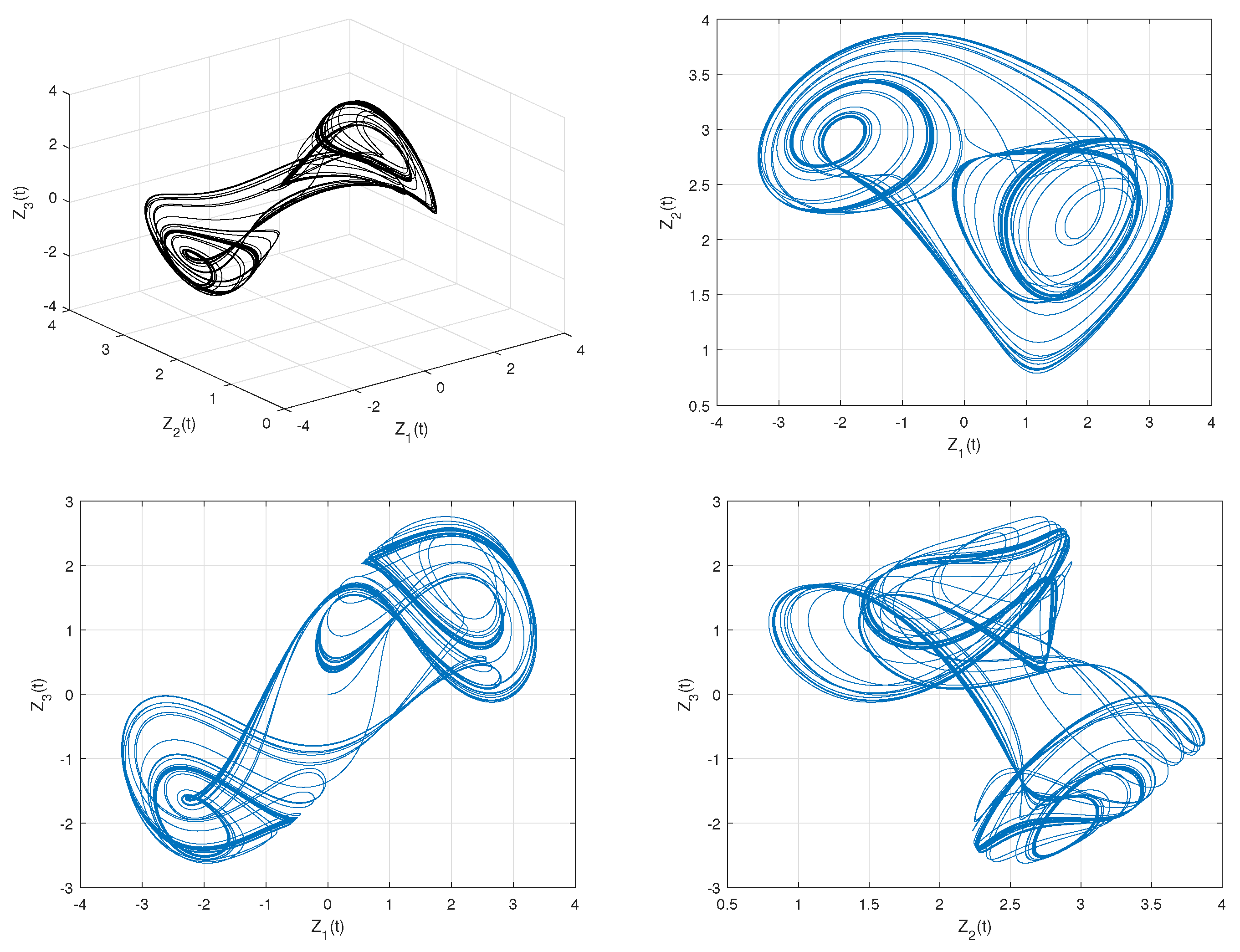
3. New Fractional Chaotic System

Introduce the fractional chaotic system as:

$$\begin{array}{c}\hfill D^q{Z}_1=Z_2+Z_3-Asin\left(Z_2\right).\\ \hfill D^q{Z}_2=-Z_1+Z_3.\\ \hfill D^q{Z}_3=-Z_1-Z_3+Bsin\left(Z_1\right).\end{array}$$

(1)

where $Z\in R^3$ are state variables for A, B$\in R$.

For $A=5,B=5$, and initial conditions $(0.000001,3,0)$ for fractional order 0.987, System (1) is chaotic as displayed in Figure 1 and Figure 2 in time series and phase plots, respectively.

4. Dynamics of the Novel System

4.1. Symmetry, Dissipativity, and Stagnation Points

The novel fractional-order chaotic system (1) does not show rotational symmetry about any axis, as the system does not remain invariant under the transformation $Z_i\to -Z_i$, $Z_j\to -Z_j$, $Z_k\to Z_k$. However, the system shows symmetry about the origin as the system remains invariant under $Z_1\to -Z_1$, $Z_2\to -Z_2$, $Z_3\to -Z_3$.

The matrix form of System (1) is:

$$\left[\begin{array}{c}{D}^q{Z}_1\\ D^q{Z}_2\\ D^q{Z}_3\end{array}\right]=\left[\begin{array}{c}{K}_1(Z_1,Z_2,Z_3)\\ K_2(Z_1,Z_2,Z_3)\\ K_3(Z_1,Z_2,Z_3)\end{array}\right]=\left[\begin{array}{c}{Z}_2+Z_3-Asin\left(Z_2\right)\\ -Z_1+Z_3\\ -Z_1-Z_3+Bsin\left(Z_1\right)\end{array}\right]$$

The divergence of vector field K is:

$$\nabla K=\frac{\partial (Z_2+Z_3-Asin\left(Z_2\right))}{\partial Z_1}+\frac{\partial (-Z_1+Z_3)}{\partial Z_2}+\frac{\partial (-Z_1-Z_3+Bsin\left(Z_1\right))}{\partial Z_3}.$$

$$=0+0-1.$$

i.e.,

$$\nabla K=-1<0.$$

Hence, System (1) is dissipative.

Equating $K_i(V_1,V_2,V_3)$ to zero for $i=1,2,3$, the stagnation points are:

$$Z_2+Z_3-Asin\left(Z_2\right)=0.$$

$$-Z_1+Z_3=0.$$

$$-Z_1-Z_3+Bsin\left(Z_1\right)=0.$$

For A = B = 5, we have stagnation point (0,0,0).

4.2. Solution of the Novel Fractional-Order Chaotic System

The novel fractional-order chaotic system is expressed as:

$$D^{q}Z\left(t\right)=\mathrm{\Psi }\left(Z\left(t\right)\right),$$

where $t\in (0,T]$ and $Z\left(0\right)=Z_o$.

Here:

$$Z=\left[\begin{array}{c}{Z}_1\\ Z_2\\ Z_3\end{array}\right],Z_o=\left[\begin{array}{c}{Z}_{1}o\\ Z_{2}o\\ Z_{3}o\end{array}\right],$$

$$\mathrm{\Psi }\left(Z\left(t\right)\right)=\left[\begin{array}{c}{Z}_2+Z_3-Asin\left(Z_2\right)\\ -Z_1+Z_3\\ -Z_1-Z_3+Bsin\left(Z_1\right)\end{array}\right].$$

The solution is examined in the region $\omega \times I$, where I = (0, T] and $\omega =\left(Z_i\right):max|Z_i|\le P$ for $i=1,2,3,P>0$, where constant P designs a boundary in the phase space.

Equivalently, the I.V.P. is:

$$Z\left(t\right)=Z_o+{\int }_0^t\mathrm{\Psi }\left(Z\left(s\right)\right)ds.$$

Let $Z_o+{\int }_0^t\mathrm{\Psi }\left(Z\left(s\right)\right)ds=$ S(Z) with $Z_1,Z_2\in R^3$.

Then:

$$S\left(Z_1\right)-S\left(Z_2\right)={\int }_0^t(\mathrm{\Psi }\left(Z_1\left(s\right)\right)-\mathrm{\Psi }\left(Z_2\left(s\right)\right))ds.$$

Hence:

$$|S\left(Z_1\right)-S\left(Z_2\right)|=|{\int }_0^t(\mathrm{\Psi }\left(Z_1\left(s\right)\right)-\mathrm{\Psi }\left(Z_2\left(s\right)\right))ds|.$$

We define the norm for $g\left(t\right)\in C(0,T]$ given by $Su{p}_{t\in (0,T]}\left|g\left(t\right)\right|$ and for matrix $G=\left[g_{ij}\left(t\right)\right]$ with $g_{ij}\left(t\right)\in C(0,T]$; define $\left|\right|G\left|\right|={\sum }_{i,j}Su{p}_{t\in (0,T]}\left|g_{ij}\left(t\right)\right|$.

$$\Rightarrow \left|\right|S\left(Z_1\right)-S\left(Z_2\right)\left|\right|\le P_1\left|\right|Z_1-Z_2\left|\right|.$$

where $P_1=Tmax(7,6,3)$.

Thus, for S(Z), $0<P_1<1$ is a contraction mapping.

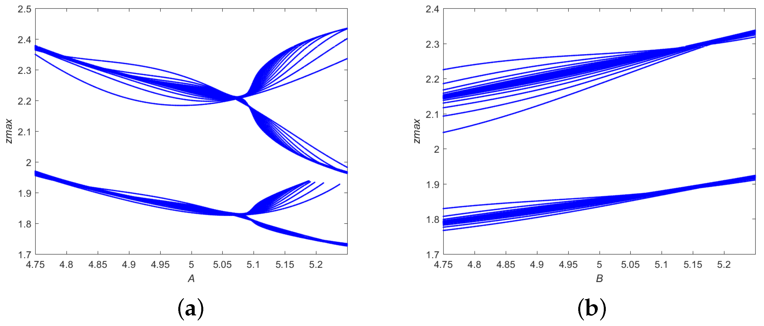
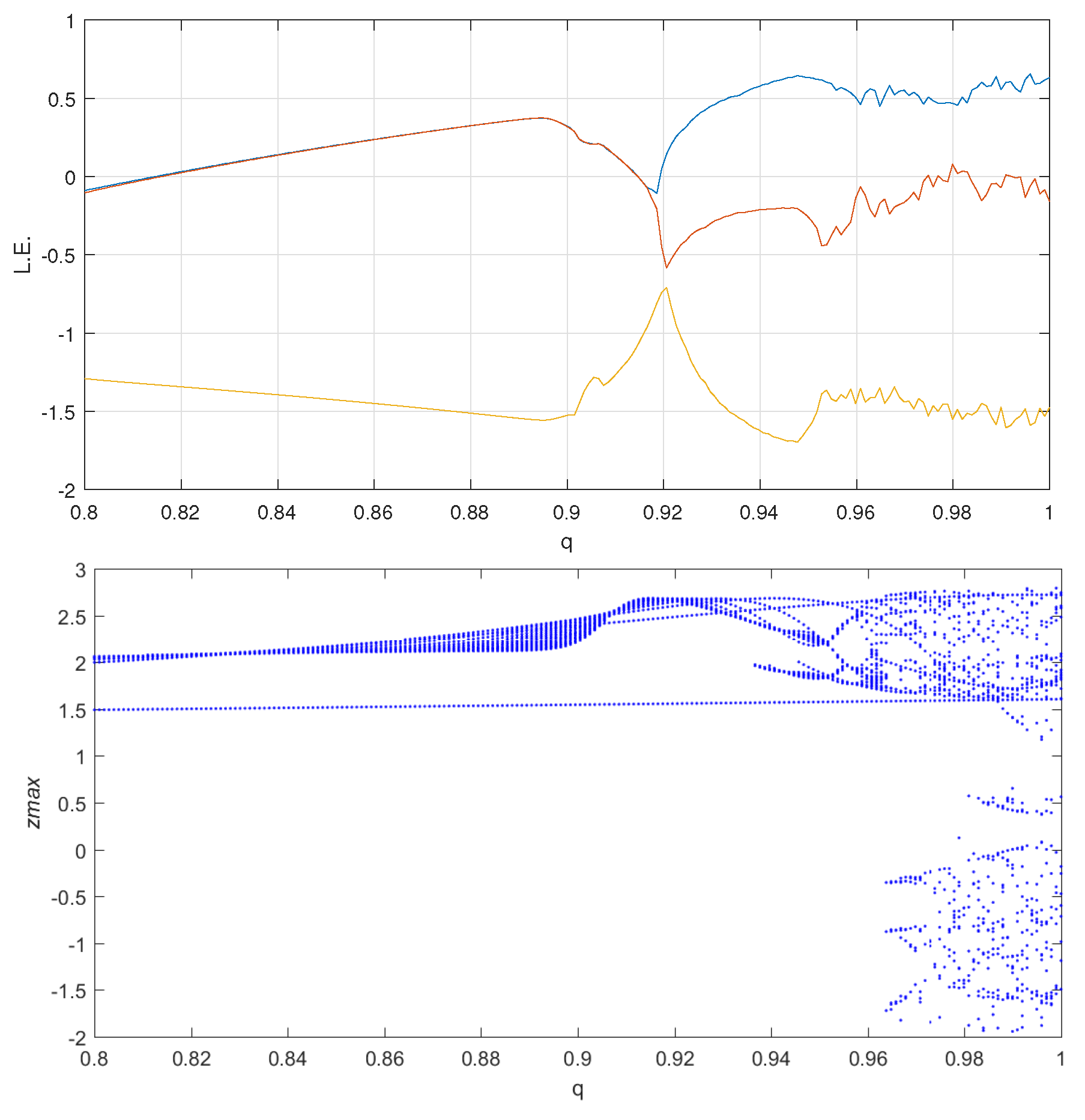
4.3. Lyapunov Dynamics and Bifurcation Analysis

With the idea of the rate of separation of closely lying trajectories in the phase space, the Lyapunov spectrum values are found. For A = B = 5 and initial conditions (0.000001, 3, 0), the Lyapunov dynamics for q = 0.987 are:

$$0.6193.$$

$$-0.0724\approx 0.$$

$$-1.6056.$$

The first component being positive confirms chaos. The dimension (K.Y.) is found by:

$$D_{YK}=p+\frac{{\sum }_{s=1}^{p}L.E{.}_s}{|L.E{.}_{p+1}|}.$$

where p is maximum number satisfying ${\sum }_{s=1}^{p}L.E{.}_s\ge 0$ and ${\sum }_{s=1}^{p+1}L.E{.}_s<0$. Therefore, the K.Y. dimension is 2.34062.

Parameter values and initial conditions have a very sensitive dependence on the system dynamics. A slight change in these values of the system can lead to drastically different dynamics. Even in the smallest neighborhood of the parameter values, the dynamics may vary in the number of equilibrium points (none, finite, countably infinite, uncountably infinite), their stability, and from the regular nature to the periodic to the chaotic nature. In bifurcation analysis, only one parameter value is varied in a slight neighborhood, while others are kept constant. In Figure 3a, A is varied in $(4.75,5.25)$ and B = 5; in Figure 3b, B is varied in $(4.75,5.25)$ and A = 5. The effect of the fractional order is given in Figure 4.

4.4. Stability of the Trivial Equilibrium Point

Clearly, the origin is the equilibrium point of the system. We check its stability by finding the Jacobian matrix as:

$$\left[\begin{array}{ccc}0& -4& 1\\ -1& 0& 1\\ 4& 0& -1\end{array}\right].$$

The eigenvalues of the above matrix are:

$${\mu }_1=1.43459+1.02145i.$$

$${\mu }_2=1.43459-1.02145i.$$

$${\mu }_3=-3.86919.$$

Here, ${\mu }_1,{\mu }_2$ are complex eigenvalues with a positive real part and ${\mu }_3$ is a negative eigenvalue, which together imply that the system is unstable.

Since all eigenvalues have a non-zero real part, the equilibrium point is hyperbolic.

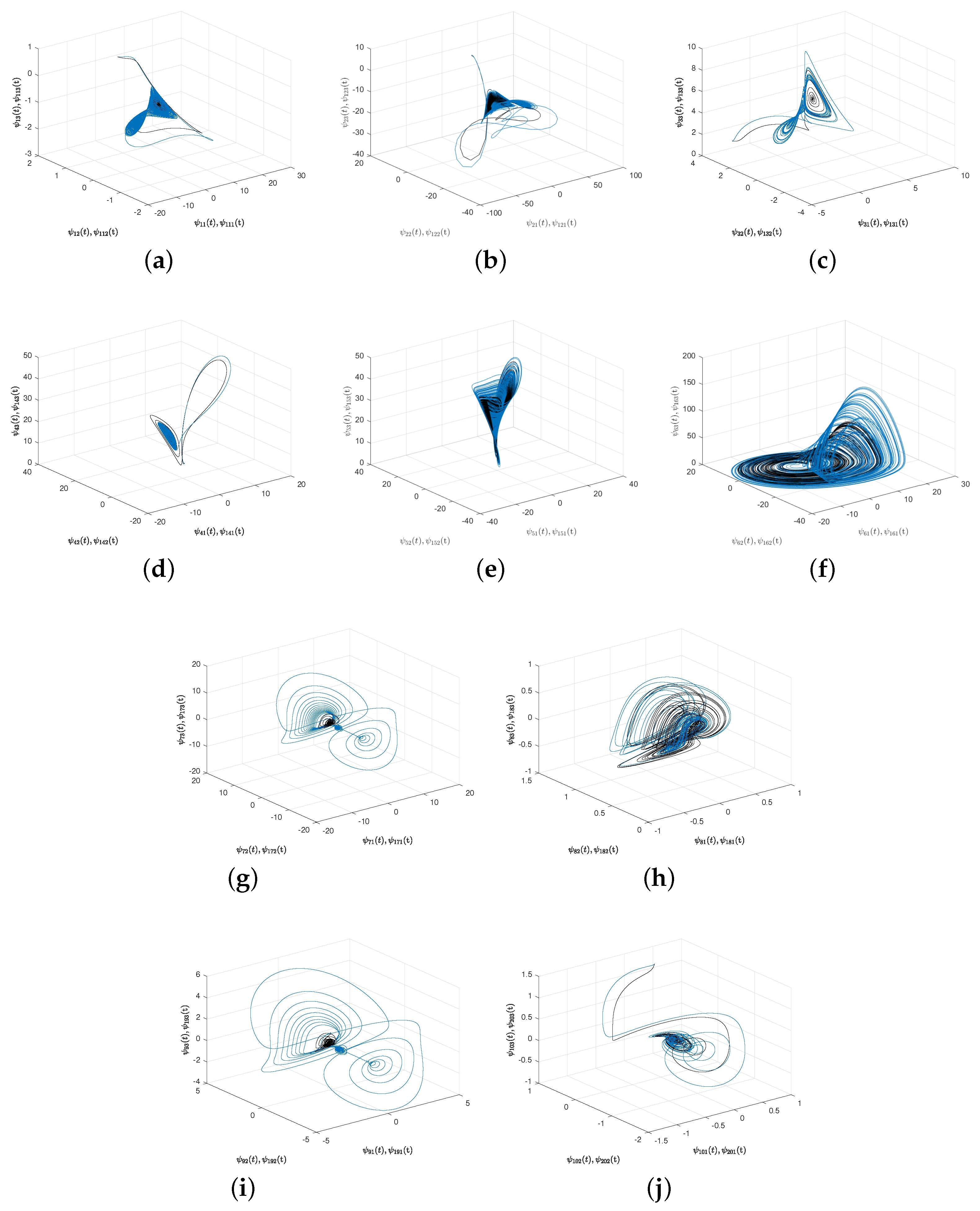
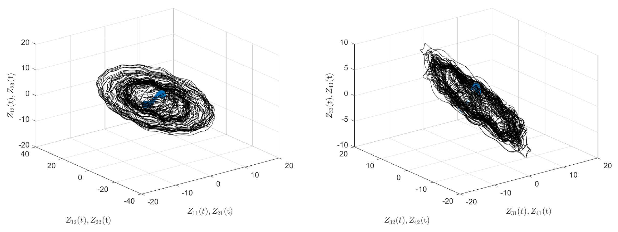
5. Dual Penta-Compound Combination Anti-Synchronization

Consider four master systems and twenty slave systems, the first ten slave systems corresponding to the first two master systems and the next ten slave systems corresponding to the next two master systems for dual penta-compound combination anti-synchronization.

Master System I:

$$\begin{array}{c}\hfill D^q{Z}_{11}=Z_{12}+Z_{13}-5sin\left(Z_{12}\right)+\overline{U_1}.\\ \hfill D^q{Z}_{12}=-Z_{11}+Z_{13}+\overline{U_2}.\\ \hfill D^q{Z}_{13}=-Z_{11}-Z_{13}+5sin\left(Z_{11}\right)+\overline{U_3}.\end{array}$$

(2)

For I.C. $(0.000001,3,0)$, q = 0.987, (2) is chaotic. Here, $\overline{U_1},\overline{U_2},\overline{U_3}$ are controllers to be designed.

Master System II:

$$\begin{array}{c}\hfill D^q{Z}_{21}=Z_{22}+Z_{23}-5sin\left(Z_{22}\right)+△H_1+D_1+\overline{U_4}.\\ \hfill D^q{Z}_{22}=-Z_{21}+Z_{23}+△H_2+D_2+\overline{U_5}.\\ \hfill D^q{Z}_{23}=-Z_{21}-Z_{23}+5sin\left(Z_{21}\right)+△H_3+D_3+\overline{U_6}.\end{array}$$

(3)

For I.C. $(0.000001,3,0)$, q = 0.987, (3) is chaotic. Here, $\overline{U_4},\overline{U_5},\overline{U_6}$ are controllers to be designed.

Master System III:

$$\begin{array}{c}\hfill D^q{Z}_{31}=Z_{32}+Z_{33}-5sin\left(Z_{32}\right)+\overline{V_1}.\\ \hfill D^q{Z}_{32}=-Z_{31}+Z_{33}+\overline{V_2}.\\ \hfill D^q{Z}_{33}=-Z_{31}-Z_{33}+5sin\left(Z_{31}\right)+\overline{V_3}.\end{array}$$

(4)

For I.C. $(0.000001,3,0)$, q = 0.95, (4) is chaotic. Here, $\overline{V_1},\overline{V_2},\overline{V_3}$ are controllers to be designed.

Master System IV:

$$\begin{array}{c}\hfill D^q{Z}_{41}=Z_{42}+Z_{43}-5sin\left(Z_{42}\right)+△H_4+D_4+\overline{V_4}.\\ \hfill D^q{Z}_{42}=-Z_{41}+Z_{43}+△H_5+D_5+\overline{V_5}.\\ \hfill D^q{Z}_{43}=-Z_{41}-Z_{43}+5sin\left(Z_{41}\right)+△H_6+D_6+\overline{V_6}.\end{array}$$

(5)

For I.C. $(0.000001,3,0)$, q = 0.95, (5) is chaotic. Here, $\overline{V_4},\overline{V_5},\overline{V_6}$ are controllers to be designed.

Phase portraits of (2)–(5) are given in Figure 5.

Slave System I:

$$\begin{array}{c}\hfill D^q{\psi }_{11}=121{\psi }_{12}-5{\psi }_{11}.\\ \hfill D^q{\psi }_{12}={\psi }_{11}{\psi }_{13}-{\psi }_{12}+{\psi }_{11}.\\ \hfill D^q{\psi }_{13}=-{\psi }_{11}{\psi }_{12}-{\psi }_{13}.\end{array}$$

(6)

For I.C. $(0.1,1.2,0.5)$ and q = 0.987, Figure 6a gives the phase diagram.

Slave System II:

$$\begin{array}{c}\hfill D^q{\psi }_{21}=83.6{\psi }_{22}-83.6{\psi }_{23}-10{\psi }_{21}.\\ \hfill D^q{\psi }_{22}={\psi }_{21}{\psi }_{23}-{\psi }_{22}+12{\psi }_{12}.\\ \hfill D^q{\psi }_{23}=-{\psi }_{21}{\psi }_{22}-12{\psi }_{21}-{\psi }_{23}.\end{array}$$

(7)

For I.C. $(-2,3,5)$ and q = 0.987, Figure 6b gives the phase diagram.

Slave System III:

$$\begin{array}{c}\hfill D^q{\psi }_{31}=-2{\psi }_{31}+{\psi }_{32}{\psi }_{33}.\\ \hfill D^q{\psi }_{32}=-2{\psi }_{32}+{\psi }_{33}{\psi }_{31}-5{\psi }_{31}.\\ \hfill D^q{\psi }_{33}=1-{\psi }_{31}{\psi }_{32}.\end{array}$$

(8)

For I.C. $(-4,2.5,2)$ with q = 0.987, Figure 6c gives the phase diagram.

Slave System IV:

$$\begin{array}{c}\hfill D^q{\psi }_{41}=10{\psi }_{42}-10{\psi }_{41}.\\ \hfill D^q{\psi }_{42}=28{\psi }_{41}-{\psi }_{42}-{\psi }_{41}{\psi }_{43}.\\ \hfill D^q{\psi }_{43}=\frac{8}{3}{\psi }_{43}+{\psi }_{41}{\psi }_{42}.\end{array}$$

(9)

For I.C. $(2,3,5)$ and q = 0.987, Figure 6d gives the phase diagram.

Slave System V:

$$\begin{array}{c}\hfill D^q{\psi }_{51}=35{\psi }_{51}-35{\psi }_{51}.\\ \hfill D^q{\psi }_{52}=-7{\psi }_{51}-{\psi }_{51}{\psi }_{53}+28{\psi }_{52}.\\ \hfill D^q{\psi }_{53}={\psi }_{51}{\psi }_{52}-3{\psi }_{53}.\end{array}$$

(10)

For I.C. $(3,4,5)$ and q = 0.987, Figure 6e gives the phase diagram.

Slave System VI:

$$\begin{array}{c}\hfill D^q{\psi }_{61}=-{\psi }_{62}-{\psi }_{63}.\\ \hfill D^q{\psi }_{62}={\psi }_{61}+0.4{\psi }_{62}.\\ \hfill D^q{\psi }_{63}=0.2+{\psi }_{63}({\psi }_{61}-10).\end{array}$$

(11)

For I.C. $(2,-6,3)$ and q = 0.987, Figure 6f gives the phase diagram.

Slave System VII:

$$\begin{array}{c}\hfill D^q{\psi }_{71}=0.7{\psi }_{71}-{\psi }_{72}{\psi }_{73}.\\ \hfill D^q{\psi }_{72}=-0.1{\psi }_{72}+{\psi }_{71}{\psi }_{73}.\\ \hfill D^q{\psi }_{73}=-0.001-{\psi }_{73}+{\psi }_{71}{\psi }_{72}+0.1{\psi }_{73}{\psi }_{72}.\end{array}$$

(12)

For I.C. $(0.1,0.2,0.3)$ and q = 0.987, Figure 6g gives the phase diagram.

Slave System VIII:

$$\begin{array}{c}\hfill D^q{\psi }_{81}=0.7{\psi }_{81}-2{\psi }_{82}{\psi }_{83}.\\ \hfill D^q{\psi }_{82}=-0.1{\psi }_{82}+2{\psi }_{81}{\psi }_{83}.\\ \hfill D^q{\psi }_{83}=-0.001-{\psi }_{83}+2{\psi }_{81}{\psi }_{82}+0.2{\psi }_{83}{\psi }_{82}.\end{array}$$

(13)

For I.C. $(0.2,0.4,0.6)$ and q = 0.987, Figure 6h gives the phase diagram.

Slave System IX:

$$\begin{array}{c}\hfill D^q{\psi }_{91}=0.7{\psi }_{91}-3{\psi }_{92}{\psi }_{93}.\\ \hfill D^q{\psi }_{92}=-0.1{\psi }_{92}+3{\psi }_{91}{\psi }_{93}.\\ \hfill D^q{\psi }_{93}=-0.001-{\psi }_{93}+3{\psi }_{91}{\psi }_{92}+0.3{\psi }_{93}{W}_{92}.\end{array}$$

(14)

For I.C. $(0.3,0.6,0.9)$ and q = 0.987, Figure 6i gives the phase diagram.

Slave System X:

$$\begin{array}{c}\hfill D^q{\psi }_{101}=0.7{\psi }_{101}-4{\psi }_{102}{\psi }_{103}.\\ \hfill D^q{\psi }_{102}=-0.1{\psi }_{102}+4{\psi }_{101}{\psi }_{103}.\\ \hfill D^q{\psi }_{103}=-0.001-{\psi }_{103}+4{\psi }_{101}{\psi }_{102}+0.4{\psi }_{103}{\psi }_{102}.\end{array}$$

(15)

For I.C. $(0.4,0.8,1.2)$ and q = 0.987, Figure 6j gives the phase diagram.

Slave System XI:

$$\begin{array}{c}\hfill D^q{\psi }_{111}=121{\psi }_{112}-5{\psi }_{111}.\\ \hfill D^q{\psi }_{112}={\psi }_{111}{\psi }_{113}-{\psi }_{112}+{\psi }_{111}.\\ \hfill D^q{\psi }_{113}=-{\psi }_{111}{\psi }_{112}-{\psi }_{113}.\end{array}$$

(16)

For I.C. $(0.1,1.2,0.5)$ and q = 0.987, Figure 6a gives the phase diagram.

Slave System XII:

$$\begin{array}{c}\hfill D^q{\psi }_{121}=83.6{\psi }_{122}-83.6{\psi }_{123}-10{\psi }_{121}.\\ \hfill D^q{\psi }_{122}={\psi }_{121}{\psi }_{123}-{\psi }_{122}+12{\psi }_{112}.\\ \hfill D^q{\psi }_{123}=-{\psi }_{121}{\psi }_{122}-12{\psi }_{121}-{\psi }_{123}.\end{array}$$

(17)

For I.C. $(-2,3,5)$ and q = 0.987, Figure 6b gives the phase diagram.

Slave System XIII:

$$\begin{array}{c}\hfill D^q{\psi }_{131}=-2{\psi }_{131}+{\psi }_{132}{\psi }_{133}.\\ \hfill D^q{\psi }_{132}=-2{\psi }_{132}+{\psi }_{133}{\psi }_{131}-5{\psi }_{131}.\\ \hfill D^q{\psi }_{133}=1-{\psi }_{131}{\psi }_{132}.\end{array}$$

(18)

For I.C. $(-4,2.5,2)$ and q = 0.987, Figure 6c gives the phase diagram.

Slave System XIV:

$$\begin{array}{c}\hfill D^q{\psi }_{141}=10{\psi }_{142}-10{\psi }_{141}.\\ \hfill D^q{\psi }_{142}=28{\psi }_{141}-{\psi }_{142}-{\psi }_{141}{\psi }_{143}.\\ \hfill D^q{\psi }_{143}=\frac{8}{3}{\psi }_{143}+{\psi }_{141}{\psi }_{142}.\end{array}$$

(19)

For I.C. $(2,3,5)$ and q = 0.987, Figure 6d gives the phase diagram.

Slave System XV:

$$\begin{array}{c}\hfill D^q{\psi }_{151}=35{\psi }_{151}-35{\psi }_{151}.\\ \hfill D^q{\psi }_{152}=-7{\psi }_{151}-{\psi }_{151}{\psi }_{153}+28{\psi }_{152}.\\ \hfill D^q{\psi }_{153}={\psi }_{151}{\psi }_{152}-3{\psi }_{153}.\end{array}$$

(20)

For I.C. $(3,4,5)$ and q = 0.987, Figure 6e gives the phase diagram.

Slave System XVI:

$$\begin{array}{c}\hfill D^q{\psi }_{161}=-{\psi }_{162}-{\psi }_{163}.\\ \hfill D^q{\psi }_{162}={\psi }_{161}+0.4{\psi }_{162}.\\ \hfill D^q{\psi }_{163}=0.2+{\psi }_{163}({\psi }_{161}-10).\end{array}$$

(21)

For I.C. $(2,-6,3)$ and q = 0.987, Figure 6f gives the phase diagram.

Slave System XVII:

$$\begin{array}{c}\hfill D^q{\psi }_{171}=0.7{\psi }_{171}-{\psi }_{172}{\psi }_{173}.\\ \hfill D^q{\psi }_{172}=-0.1{\psi }_{172}+{\psi }_{171}{\psi }_{173}.\\ \hfill D^q{\psi }_{173}=-0.001-{\psi }_{173}+{\psi }_{171}{\psi }_{172}+0.1{\psi }_{173}{\psi }_{172}.\end{array}$$

(22)

For I.C. $(0.1,0.2,0.3)$ and q = 0.987, Figure 6g gives the phase diagram.

Slave System XVIII:

$$\begin{array}{c}\hfill D^q{\psi }_{181}=0.7{\psi }_{181}-2{\psi }_{182}{\psi }_{183}.\\ \hfill D^q{\psi }_{182}=-0.1{\psi }_{182}+2{\psi }_{181}{\psi }_{183}.\\ \hfill D^q{\psi }_{183}=-0.001-{\psi }_{183}+2{\psi }_{181}{\psi }_{182}+0.2{\psi }_{183}{\psi }_{82}.\end{array}$$

(23)

For I.C. $(0.2,0.4,9.6)$ and q = 0.987, Figure 6h gives the phase diagram.

Slave System XIX:

$$\begin{array}{c}\hfill D^q{\psi }_{191}=0.7{\psi }_{191}-3{\psi }_{192}{\psi }_{193}.\\ \hfill D^q{\psi }_{192}=-0.1{\psi }_{192}+3{\psi }_{191}{\psi }_{193}.\\ \hfill D^q{\psi }_{193}=-0.001-{\psi }_{193}+3{\psi }_{191}{\psi }_{192}+0.3{\psi }_{193}{W}_{92}.\end{array}$$

(24)

For I.C. $(0.3,0.6,0.9)$ and q = 0.987, Figure 6i gives the phase diagram.

Slave System XX:

$$\begin{array}{c}\hfill D^q{\psi }_{201}=0.7{\psi }_{201}-4{\psi }_{202}{\psi }_{203}.\\ \hfill D^q{\psi }_{202}=-0.1{\psi }_{202}+4{\psi }_{201}{\psi }_{203}.\\ \hfill D^q{\psi }_{203}=-0.001-{\psi }_{203}+4{\psi }_{201}{\psi }_{202}+0.4{\psi }_{203}{\psi }_{202}.\end{array}$$

(25)

For I.C. $(0.4,0.8,1.2)$ and q = 0.987, Figure 6j gives the phase diagram.

Define the dual penta-compound combination anti-synchronization error:

$$\begin{array}{c}\hfill E_1=(Z_{11}+Z_{21})+({\psi }_{11}+{\psi }_{21})({\psi }_{31}+{\psi }_{41})({\psi }_{51}+{\psi }_{61})({\psi }_{71}+{\psi }_{81})({\psi }_{91}+{\psi }_{101}).\\ \hfill E_2=(Z_{12}+Z_{22})+({\psi }_{12}+{\psi }_{22})({\psi }_{32}+{\psi }_{42})({\psi }_{52}+{\psi }_{62})({\psi }_{72}+{\psi }_{82})({\psi }_{92}+{\psi }_{102}).\\ \hfill E_3=(Z_{13}+Z_{23})+({\psi }_{13}+{\psi }_{23})({\psi }_{33}+{\psi }_{43})({\psi }_{53}+{\psi }_{63})({\psi }_{73}+{\psi }_{83})({\psi }_{93}+{\psi }_{103}).\\ \hfill E_4=(Z_{31}+Z_{41})+({\psi }_{111}+{\psi }_{121})({\psi }_{131}+{\psi }_{141})({\psi }_{151}+{\psi }_{161})({\psi }_{171}+{\psi }_{181})({\psi }_{191}+{\psi }_{201}).\\ \hfill E_5=(Z_{32}+Z_{42})+({\psi }_{112}+{\psi }_{122})({\psi }_{132}+{\psi }_{142})({\psi }_{152}+{\psi }_{162})({\psi }_{172}+{\psi }_{182})({\psi }_{192}+{\psi }_{202}).\\ \hfill E_6=(Z_{33}+Z_{43})+({\psi }_{113}+{\psi }_{123})({\psi }_{133}+{\psi }_{143})({\psi }_{153}+{\psi }_{163})({\psi }_{173}+{\psi }_{183})({\psi }_{193}+{\psi }_{203}).\end{array}$$

(26)

Differentiating (26), from (2)–(25), we have:

$$\begin{array}{cc}\hfill D^q{E}_1& =(Z_{12}+Z_{13}-5sin\left(Z_{12}\right)+\overline{U_1}+Z_{22}+Z_{23}-5sin\left(Z_{22}\right)+△H_1+D_1+\overline{U_4})+(121{\psi }_{12}\hfill \\ & -5{\psi }_{11}+83.6{\psi }_{22}-83.6{\psi }_{23}-10{\psi }_{21})({\psi }_{31}+{\psi }_{41})({\psi }_{51}+{\psi }_{61})({\psi }_{71}+{\psi }_{81})({\psi }_{91}+{\psi }_{101})+\hfill \\ & ({\psi }_{11}+{\psi }_{21})(-2{\psi }_{31}+{\psi }_{32}{\psi }_{33}+10{\psi }_{42}-10{\psi }_{41})({\psi }_{51}+{\psi }_{61})({\psi }_{71}+{\psi }_{81})({\psi }_{91}+{\psi }_{101})+({\psi }_{11}\hfill \\ & +{\psi }_{21})({\psi }_{31}+{\psi }_{41})(35{\psi }_{51}-35{\psi }_{51}+-{\psi }_{62}-{\psi }_{63})({\psi }_{71}+{\psi }_{81})({\psi }_{91}+{\psi }_{101})+({\psi }_{11}+{\psi }_{21})\hfill \\ & ({\psi }_{31}+{\psi }_{41})({\psi }_{51}+{\psi }_{61})(0.7{\psi }_{71}-{\psi }_{72}{\psi }_{73}+0.7{\psi }_{81}-2{\psi }_{82}{\psi }_{83})({\psi }_{91}+{\psi }_{101})+({\psi }_{11}\hfill \\ & +{\psi }_{21})({\psi }_{31}+{\psi }_{41})({\psi }_{51}+{\psi }_{61})({\psi }_{71}+{\psi }_{81})(0.7{\psi }_{91}-3{\psi }_{92}{\psi }_{93}+0.7{\psi }_{101}-4{\psi }_{102}{\psi }_{103}).\hfill \\ \hfill D^q{E}_2& =(-Z_{11}+Z_{13}+\overline{U_2}-Z_{21}+Z_{23}+△H_2+D_2+\overline{U_5})+({\psi }_{11}{\psi }_{13}-{\psi }_{12}+{\psi }_{11}+{\psi }_{21}{\psi }_{23}-\hfill \\ & {\psi }_{22}+12{\psi }_{12})({\psi }_{32}+{\psi }_{42})({\psi }_{52}+{\psi }_{62})({\psi }_{72}+{\psi }_{82})({\psi }_{92}+{\psi }_{102})+({\psi }_{12}+{\psi }_{22})(-2{\psi }_{32}+\hfill \\ & {\psi }_{33}{\psi }_{31}-5{\psi }_{31}+28{\psi }_{41}-{\psi }_{42}-{\psi }_{41}{\psi }_{43})({\psi }_{52}+{\psi }_{62})({\psi }_{72}+{\psi }_{82})({\psi }_{92}+{\psi }_{102})+({\psi }_{12}+{\psi }_{22})\hfill \\ & ({\psi }_{32}+{\psi }_{42})(-7{\psi }_{51}-{\psi }_{51}{\psi }_{53}+28{\psi }_{52}+{\psi }_{61}+0.4{\psi }_{62})({\psi }_{72}+{\psi }_{82})({\psi }_{92}+{\psi }_{102})+({\psi }_{12}+\hfill \\ & {\psi }_{22})({\psi }_{32}+{\psi }_{42})({\psi }_{52}+{\psi }_{62})(-0.1{\psi }_{72}+{\psi }_{71}{\psi }_{73}-0.1{\psi }_{82}+2{\psi }_{81}{\psi }_{83})({\psi }_{92}+{\psi }_{102})+({\psi }_{12}\hfill \\ & +{\psi }_{22})({\psi }_{32}+{\psi }_{42})({\psi }_{52}+{\psi }_{62})({\psi }_{72}+{\psi }_{82})(-0.1{\psi }_{92}+3{\psi }_{91}{\psi }_{93}+-0.1{\psi }_{102}+4{\psi }_{101}{\psi }_{103}).\hfill \\ \hfill D^q{E}_3& =(-Z_{11}-Z_{13}+5sin\left(Z_{11}\right)+\overline{U_3}-Z_{21}-Z_{23}+5sin\left(Z_{21}\right)+△H_3+D_3+\overline{U_6})-({\psi }_{11}{\psi }_{12}\hfill \\ & -{\psi }_{13}-{\psi }_{21}{\psi }_{22}-12{\psi }_{21}-{\psi }_{23})({\psi }_{33}+{\psi }_{43})({\psi }_{53}+{\psi }_{63})({\psi }_{73}+{\psi }_{83})({\psi }_{93}+{\psi }_{103})+({\psi }_{13}\hfill \\ & +{\psi }_{23})(1-{\psi }_{31}{\psi }_{32}+\frac{8}{3}{\psi }_{43}+{\psi }_{41}{\psi }_{42})({\psi }_{53}+{\psi }_{63})({\psi }_{73}+{\psi }_{83})({\psi }_{93}+{\psi }_{103})+({\psi }_{13}+{\psi }_{23})\hfill \\ & ({\psi }_{33}+{\psi }_{43})({\psi }_{51}{\psi }_{52}-3{\psi }_{53}+0.2+{\psi }_{63}({\psi }_{61}-10))({\psi }_{73}+{\psi }_{83})({\psi }_{93}+{\psi }_{103})+({\psi }_{13}+{\psi }_{23})\hfill \\ & ({\psi }_{33}+{\psi }_{43})({\psi }_{53}+{\psi }_{63})(-0.001-{\psi }_{73}+{\psi }_{71}{\psi }_{72}+0.1{\psi }_{73}{\psi }_{72}-0.001-{\psi }_{83}+2{\psi }_{81}{\psi }_{82}+\hfill \\ & 0.2{\psi }_{83}{\psi }_{82})({\psi }_{93}+{\psi }_{103})+({\psi }_{13}+{\psi }_{23})({\psi }_{33}+{\psi }_{43})({\psi }_{53}+{\psi }_{63})({\psi }_{73}+{\psi }_{83})\hfill \\ & (-0.001-{\psi }_{93}+3{\psi }_{91}{\psi }_{92}+0.3{\psi }_{93}{W}_{92}-0.001-{\psi }_{103}+4{\psi }_{101}{\psi }_{102}+0.4{\psi }_{103}{\psi }_{102}).\hfill \\ \hfill D^q{E}_4& =(Z_{32}+Z_{33}-5sin\left(Z_{32}\right)+\overline{V_1}+Z_{42}+Z_{43}-5sin\left(Z_{42}\right)+△H_4+D_4+\overline{V_4})+(121{\psi }_{112}\hfill \\ & -5{\psi }_{111}+83.6{\psi }_{122}-83.6{\psi }_{123}-10{\psi }_{121}\left)({\psi }_{131}+{\psi }_{141})({\psi }_{151}+{\psi }_{161})({\psi }_{171}+{\psi }_{181})\right({\psi }_{191}\hfill \\ & +{\psi }_{201})+({\psi }_{111}+{\psi }_{121})(-2{\psi }_{131}+{\psi }_{132}{\psi }_{133}+10{\psi }_{142}-10{\psi }_{141})({\psi }_{151}+{\psi }_{161})({\psi }_{171}+{\psi }_{181})\hfill \\ & ({\psi }_{191}+{\psi }_{201})+({\psi }_{111}+{\psi }_{121})({\psi }_{131}+{\psi }_{141})(35{\psi }_{151}-35{\psi }_{151}-{\psi }_{162}-{\psi }_{163})({\psi }_{171}+{\psi }_{181})\hfill \\ & ({\psi }_{191}+{\psi }_{201})+({\psi }_{111}+{\psi }_{121})({\psi }_{131}+{\psi }_{141})({\psi }_{151}+{\psi }_{161})(0.7{\psi }_{171}-{\psi }_{172}{\psi }_{173}+0.7{\psi }_{181}\hfill \\ & -2{\psi }_{182}{\psi }_{183})({\psi }_{191}+{\psi }_{201})+({\psi }_{111}+{\psi }_{121})({\psi }_{131}+{\psi }_{141})({\psi }_{151}+{\psi }_{161})({\psi }_{171}+{\psi }_{181})\hfill \\ & (0.7{\psi }_{191}-3{\psi }_{192}{\psi }_{193}+0.7{\psi }_{201}-4{\psi }_{202}{\psi }_{203}).\hfill \\ \hfill D^q{E}_5& =(-Z_{31}+Z_{33}+\overline{V_2}-Z_{41}+Z_{43}+△H_5+D_5+\overline{V_5})+({\psi }_{111}{\psi }_{113}-{\psi }_{112}+{\psi }_{111}+{\psi }_{121}{\psi }_{123}\hfill \\ & -{\psi }_{122}+12{\psi }_{112})({\psi }_{132}+{\psi }_{142})({\psi }_{152}+{\psi }_{162})({\psi }_{172}+{\psi }_{182})({\psi }_{192}+{\psi }_{202})+({\psi }_{112}+{\psi }_{122})\hfill \\ & (-2{\psi }_{132}+{\psi }_{133}{\psi }_{131}-5{\psi }_{131}+28{\psi }_{141}-{\psi }_{142}-{\psi }_{141}{\psi }_{143})({\psi }_{152}+{\psi }_{162})({\psi }_{172}+{\psi }_{182})({\psi }_{192}+\hfill \\ & {\psi }_{202})+({\psi }_{112}+{\psi }_{122})({\psi }_{132}+{\psi }_{142})(-7{\psi }_{151}-{\psi }_{151}{\psi }_{153}+28{\psi }_{152}+{\psi }_{161}+0.4{\psi }_{162})({\psi }_{172}\hfill \\ & +{\psi }_{182})({\psi }_{192}+{\psi }_{202})+({\psi }_{112}+{\psi }_{122})({\psi }_{132}+{\psi }_{142})({\psi }_{152}+{\psi }_{162})(-0.1{\psi }_{172}+{\psi }_{171}{\psi }_{173}\hfill \\ & -0.1{\psi }_{182}+2{\psi }_{181}{\psi }_{183})({\psi }_{192}+{\psi }_{202})+({\psi }_{112}+{\psi }_{122})({\psi }_{132}+{\psi }_{142})({\psi }_{152}+{\psi }_{162})({\psi }_{172}\hfill \\ & +{\psi }_{182})(-0.1{\psi }_{192}+3{\psi }_{191}{\psi }_{193}-0.1{\psi }_{202}+4{\psi }_{201}{\psi }_{203}).\hfill \\ \hfill D^q{E}_6& =(-Z_{31}-Z_{33}+5sin\left(Z_{31}\right)+\overline{V_3}+-Z_{41}-Z_{43}+5sin\left(Z_{41}\right)+△H_6+D_6+\overline{V_6})+(-{\psi }_{111}\hfill \\ & {\psi }_{112}-{\psi }_{113}-{\psi }_{121}{\psi }_{122}-12{\psi }_{121}-{\psi }_{123}\left)({\psi }_{133}+{\psi }_{143})({\psi }_{153}+{\psi }_{163})({\psi }_{173}+{\psi }_{183})\right({\psi }_{193}\hfill \\ & +{\psi }_{203})+({\psi }_{113}+{\psi }_{123})(1-{\psi }_{131}{\psi }_{132}+\frac{8}{3}{\psi }_{143}+{\psi }_{141}{\psi }_{142})({\psi }_{153}+{\psi }_{163})({\psi }_{173}+{\psi }_{183})({\psi }_{193}\hfill \\ & +{\psi }_{203})+({\psi }_{113}+{\psi }_{123})({\psi }_{133}+{\psi }_{143})({\psi }_{151}{\psi }_{152}-3{\psi }_{153}+0.2+{\psi }_{163}({\psi }_{161}-10))({\psi }_{173}+\hfill \\ & {\psi }_{183})({\psi }_{193}+{\psi }_{203})+({\psi }_{113}+{\psi }_{123})({\psi }_{133}+{\psi }_{143})({\psi }_{153}+{\psi }_{163})(-0.001-{\psi }_{173}+{\psi }_{171}{\psi }_{172}\hfill \\ & +0.1{\psi }_{173}{\psi }_{172}-0.001-{\psi }_{183}+2{\psi }_{181}{\psi }_{182}+0.2{\psi }_{183}{\psi }_{182})({\psi }_{193}+{\psi }_{203})+({\psi }_{113}+{\psi }_{123})\hfill \\ & ({\psi }_{133}+{\psi }_{143})({\psi }_{153}+{\psi }_{163})({\psi }_{173}+{\psi }_{183})(-0.001-{\psi }_{193}+3{\psi }_{191}{\psi }_{192}+0.3{\psi }_{193}{W}_{192}\hfill \\ & -0.001-{\psi }_{203}+4{\psi }_{201}{\psi }_{202}+0.4{\psi }_{203}{\psi }_{202}).\hfill \end{array}$$

(27)

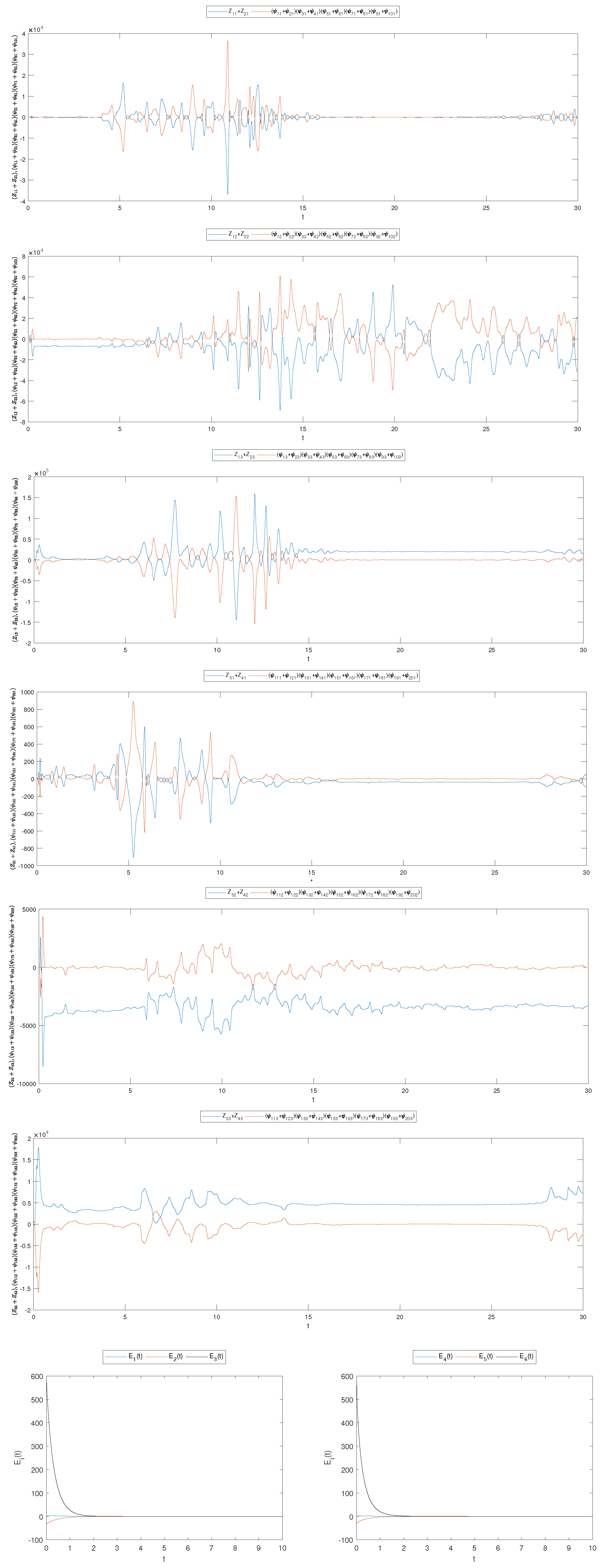
5.1. Via Non-Linear Control

Design the non-linear control functions:

$$\begin{array}{cc}\hfill \overline{U_1}& =-Z_{12}-Z_{13}+5sin\left(Z_{12}\right)-(121{\psi }_{12}-5{\psi }_{11}+83.6{\psi }_{22}-83.6{\psi }_{23}-10{\psi }_{21})({\psi }_{31}+{\psi }_{41})({\psi }_{51}\hfill \\ & +{\psi }_{61})({\psi }_{71}+{\psi }_{81})({\psi }_{91}+{\psi }_{101})-({\psi }_{11}+{\psi }_{21})({\psi }_{31}+{\psi }_{41})(35{\psi }_{51}-35{\psi }_{51}+-{\psi }_{62}-{\psi }_{63})\hfill \\ & ({\psi }_{71}+{\psi }_{81})({\psi }_{91}+{\psi }_{101})-({\psi }_{11}+{\psi }_{21})({\psi }_{31}+{\psi }_{41})({\psi }_{51}+{\psi }_{61})({\psi }_{71}+{\psi }_{81})(0.7{\psi }_{91}\hfill \\ & -3{\psi }_{92}{\psi }_{93}+0.7{\psi }_{101}-4{\psi }_{102}{\psi }_{103}).\hfill \\ \hfill \overline{U_2}& =Z_{11}-Z_{13}-({\psi }_{11}{\psi }_{13}-{\psi }_{12}+{\psi }_{11}+{\psi }_{21}{\psi }_{23}-{\psi }_{22}+12{\psi }_{12})({\psi }_{32}+{\psi }_{42})({\psi }_{52}+{\psi }_{62})({\psi }_{72}\hfill \\ & +{\psi }_{82})({\psi }_{92}+{\psi }_{102})-({\psi }_{12}+{\psi }_{22})({\psi }_{32}+{\psi }_{42})(-7{\psi }_{51}-{\psi }_{51}{\psi }_{53}+28{\psi }_{52}+{\psi }_{61}+0.4{\psi }_{62})({\psi }_{72}\hfill \\ & +{\psi }_{82})({\psi }_{92}+{\psi }_{102})-({\psi }_{12}+{\psi }_{22})({\psi }_{32}+{\psi }_{42})({\psi }_{52}+{\psi }_{62})({\psi }_{72}+{\psi }_{82})(-0.1{\psi }_{92}+3{\psi }_{91}{\psi }_{93}\hfill \\ & -0.1{\psi }_{102}+4{\psi }_{101}{\psi }_{103}).\hfill \\ \hfill \overline{U_3}& =Z_{11}+Z_{13}-5sin\left(Z_{11}\right)+(+{\psi }_{11}{\psi }_{12}+{\psi }_{13}+{\psi }_{21}{\psi }_{22}-12{\psi }_{21}+{\psi }_{23})({\psi }_{33}+{\psi }_{43})({\psi }_{53}+{\psi }_{63})\hfill \\ & ({\psi }_{73}+{\psi }_{83})({\psi }_{93}+{\psi }_{103})-({\psi }_{13}+{\psi }_{23})({\psi }_{33}+{\psi }_{43})({\psi }_{51}{\psi }_{52}-3{\psi }_{53}+0.2+{\psi }_{63}({\psi }_{61}-10))({\psi }_{73}\hfill \\ & +{\psi }_{83})({\psi }_{93}+{\psi }_{103})-({\psi }_{13}+{\psi }_{23})({\psi }_{33}+{\psi }_{43})({\psi }_{53}+{\psi }_{63})({\psi }_{73}+{\psi }_{83})(-0.001-{\psi }_{93}\hfill \\ & +3{\psi }_{91}{\psi }_{92}+0.3{\psi }_{93}{\psi }_{92}-0.001-{\psi }_{103}+4{\psi }_{101}{\psi }_{102}+0.4{\psi }_{103}{\psi }_{102}).\hfill \\ \hfill \overline{U_4}& =-Z_{22}-Z_{23}+5sin\left(Z_{22}\right)-7sin\left(t\right)-({\psi }_{11}+{\psi }_{21})(-2{\psi }_{31}+{\psi }_{32}{\psi }_{33}+10{\psi }_{42}-10{\psi }_{41})({\psi }_{51}\hfill \\ & +{\psi }_{61})({\psi }_{71}+{\psi }_{81})({\psi }_{91}+{\psi }_{101})-({\psi }_{11}+{\psi }_{21})({\psi }_{31}+{\psi }_{41})({\psi }_{51}+{\psi }_{61})(0.7{\psi }_{71}-{\psi }_{72}{\psi }_{73}\hfill \\ & +0.7{\psi }_{81}-2{\psi }_{82}{\psi }_{83})({\psi }_{91}+{\psi }_{101})-E_1.\hfill \\ \hfill \overline{U_5}& =Z_{21}-Z_{23}-sin\left(7t\right)-({\psi }_{12}+{\psi }_{22})(-2{\psi }_{32}+{\psi }_{33}{\psi }_{31}-5{\psi }_{31}+28{\psi }_{41}-{\psi }_{42}-{\psi }_{41}{\psi }_{43})({\psi }_{52}\hfill \\ & +{\psi }_{62})({\psi }_{72}+{\psi }_{82})({\psi }_{92}+{\psi }_{102})-({\psi }_{12}+{\psi }_{22})({\psi }_{32}+{\psi }_{42})({\psi }_{52}+{\psi }_{62})(-0.1{\psi }_{72}+{\psi }_{71}{\psi }_{73}\hfill \\ & -0.1{\psi }_{82}+2{\psi }_{81}{\psi }_{83})({\psi }_{92}+{\psi }_{102})-2E_2.\hfill \\ \hfill \overline{U_6}& =Z_{21}+Z_{23}-5sin\left(Z_{21}\right)-cos\left(Z_{21}\right)-({\psi }_{13}+{\psi }_{23})(1-{\psi }_{31}{\psi }_{32}+\frac{8}{3}{\psi }_{43}+{\psi }_{41}{\psi }_{42})({\psi }_{53}+{\psi }_{63})\hfill \\ & ({\psi }_{73}+{\psi }_{83})({\psi }_{93}+{\psi }_{103})-({\psi }_{13}+{\psi }_{23})({\psi }_{33}+{\psi }_{43})({\psi }_{53}+{\psi }_{63})(-0.001-{\psi }_{73}+{\psi }_{71}{\psi }_{72}\hfill \\ & +0.1{\psi }_{73}{\psi }_{72}-0.001-{\psi }_{83}+2{\psi }_{81}{\psi }_{82}+0.2{\psi }_{83}{\psi }_{82})({\psi }_{93}+{\psi }_{103})-3E_3.\hfill \\ \hfill \overline{V_1}& =-Z_{32}-Z_{33}+5sin\left(Z_{32}\right)-(121{\psi }_{112}-5{\psi }_{111}+83.6{\psi }_{122}-83.6{\psi }_{123}-10{\psi }_{121})({\psi }_{131}+{\psi }_{141})\hfill \\ & ({\psi }_{151}+{\psi }_{161})({\psi }_{171}+{\psi }_{181})({\psi }_{191}+{\psi }_{201})-({\psi }_{111}+{\psi }_{121})({\psi }_{131}+{\psi }_{141})(35{\psi }_{151}-35{\psi }_{151}-{\psi }_{162}\hfill \\ & -{\psi }_{163})({\psi }_{171}+{\psi }_{181})({\psi }_{191}+{\psi }_{201})-({\psi }_{111}+{\psi }_{121})({\psi }_{131}+{\psi }_{141})({\psi }_{151}+{\psi }_{161})({\psi }_{171}+{\psi }_{181})\hfill \\ & (0.7{\psi }_{191}-3{\psi }_{192}{\psi }_{193}+0.7{\psi }_{201}-4{\psi }_{202}{\psi }_{203}).\hfill \\ \hfill \overline{V_2}& =Z_{31}-Z_{33}-({\psi }_{111}{\psi }_{113}-{\psi }_{112}+{\psi }_{111}+{\psi }_{121}{\psi }_{123}-{\psi }_{122}+12{\psi }_{112})({\psi }_{132}+{\psi }_{142})({\psi }_{152}\hfill \\ & +{\psi }_{162})({\psi }_{172}+{\psi }_{182})({\psi }_{192}+{\psi }_{202})-({\psi }_{112}+{\psi }_{122})({\psi }_{132}+{\psi }_{142})(-7{\psi }_{151}-{\psi }_{151}{\psi }_{153}+28{\psi }_{152}\hfill \\ & +{\psi }_{161}+0.4{\psi }_{162})({\psi }_{172}+{\psi }_{182})({\psi }_{192}+{\psi }_{202})-({\psi }_{112}+{\psi }_{122})({\psi }_{132}+{\psi }_{142})({\psi }_{152}+{\psi }_{162})\hfill \\ & ({\psi }_{172}+{\psi }_{182})(-0.1{\psi }_{192}+3{\psi }_{191}{\psi }_{193}-0.1{\psi }_{202}+4{\psi }_{201}{\psi }_{203}).\hfill \\ \hfill \overline{V_3}& =Z_{31}+Z_{33}-5sin\left(Z_{11}\right)-(-{\psi }_{111}{\psi }_{112}-{\psi }_{113}+-{\psi }_{121}{\psi }_{122}-12{\psi }_{121}-{\psi }_{123})({\psi }_{133}+{\psi }_{143})\hfill \\ & ({\psi }_{153}+{\psi }_{163})({\psi }_{173}+{\psi }_{183})({\psi }_{193}+{\psi }_{203})-({\psi }_{113}+{\psi }_{123})({\psi }_{133}+{\psi }_{143})({\psi }_{151}{\psi }_{152}-3{\psi }_{153}\hfill \\ & +0.2+{\psi }_{163}({\psi }_{161}-10))({\psi }_{173}+{\psi }_{183})({\psi }_{193}+{\psi }_{203})-({\psi }_{113}+{\psi }_{123})({\psi }_{133}+{\psi }_{143})({\psi }_{153}\hfill \\ & +{\psi }_{163}\left)({\psi }_{173}+{\psi }_{183})\right(-0.001-{\psi }_{193}+3{\psi }_{191}{\psi }_{192}+0.3{\psi }_{193}{W}_{192}-0.001-{\psi }_{203}\hfill \\ & +4{\psi }_{201}{\psi }_{202}+0.4{\psi }_{203}{\psi }_{202}).\hfill \\ \hfill \overline{V_4}& =-Z_{42}-Z_{43}+5sin\left(Z_{42}\right)-7sin\left(t\right)-({\psi }_{111}+{\psi }_{121})(-2{\psi }_{131}+{\psi }_{132}{\psi }_{133}+10{\psi }_{142}-10{\psi }_{141})\hfill \\ & ({\psi }_{151}+{\psi }_{161})({\psi }_{171}+{\psi }_{181})({\psi }_{191}+{\psi }_{201})-({\psi }_{111}+{\psi }_{121})({\psi }_{131}+{\psi }_{141})({\psi }_{151}+{\psi }_{161})(0.7{\psi }_{171}-{\psi }_{172}{\psi }_{173}\hfill \\ & +0.7{\psi }_{181}-2{\psi }_{182}{\psi }_{183})({\psi }_{191}+{\psi }_{201})-E_4.\hfill \\ \hfill \overline{V_5}& =Z_{41}-Z_{43}-sin\left(7t\right)-({\psi }_{112}+{\psi }_{122})(-2{\psi }_{132}+{\psi }_{133}{\psi }_{131}-5{\psi }_{131}+28{\psi }_{141}-{\psi }_{142}\hfill \\ & -{\psi }_{141}{\psi }_{143})({\psi }_{152}+{\psi }_{162})({\psi }_{172}+{\psi }_{182})({\psi }_{192}+{\psi }_{202})-({\psi }_{112}+{\psi }_{122})({\psi }_{132}+{\psi }_{142})({\psi }_{152}\hfill \\ & +{\psi }_{162})(-0.1{\psi }_{172}+{\psi }_{171}{\psi }_{173}-0.1{\psi }_{182}+2{\psi }_{181}{\psi }_{183})({\psi }_{192}+{\psi }_{202})-2E_5.\hfill \end{array}$$

(28)

$$\begin{array}{cc}\hfill \overline{V_6}& =Z_{41}+Z_{43}-5sin\left(Z_{41}\right)-cos\left(Z_{41}\right)-({\psi }_{113}+{\psi }_{123})(1-{\psi }_{131}{\psi }_{132}+\frac{8}{3}{\psi }_{143}+{\psi }_{141}{\psi }_{142})\hfill \\ & ({\psi }_{153}+{\psi }_{163})({\psi }_{173}+{\psi }_{183})({\psi }_{193}+{\psi }_{203})-({\psi }_{113}+{\psi }_{123})({\psi }_{133}+{\psi }_{143})({\psi }_{153}+{\psi }_{163})(-0.001-{\psi }_{173}+{\psi }_{171}{\psi }_{172}\hfill \\ & +0.1{\psi }_{173}{\psi }_{172}-0.001-{\psi }_{183}+2{\psi }_{181}{\psi }_{182}+0.2{\psi }_{183}{\psi }_{182})({\psi }_{193}+{\psi }_{203})-3E_6.\hfill \end{array}$$

Substituting (28) into (27):

$$D^Q{E}_i=-E_i.$$

Consider the Lyapunov function as:

$$V\left(E\left(t\right)\right)=\frac{1}{2}({E_1}^2+{E_2}^2+{E_3}^2+{E_4}^2+{E_5}^2+{E_6}^2).$$

Differentiating:

$$D^{Q}V\left(E\right(t\left)\right)\le \sum _{i=1}^6{E}_i(-E_i).$$

$$=-\sum _{i=1}^6{E_i}^2.$$

Using the stability theory of Lyapunov, $E_i\to 0$ for i = 1, 2, 3, 4, 5, 6 as $t\to \infty$, implying dual penta-compound combination anti-synchronization.

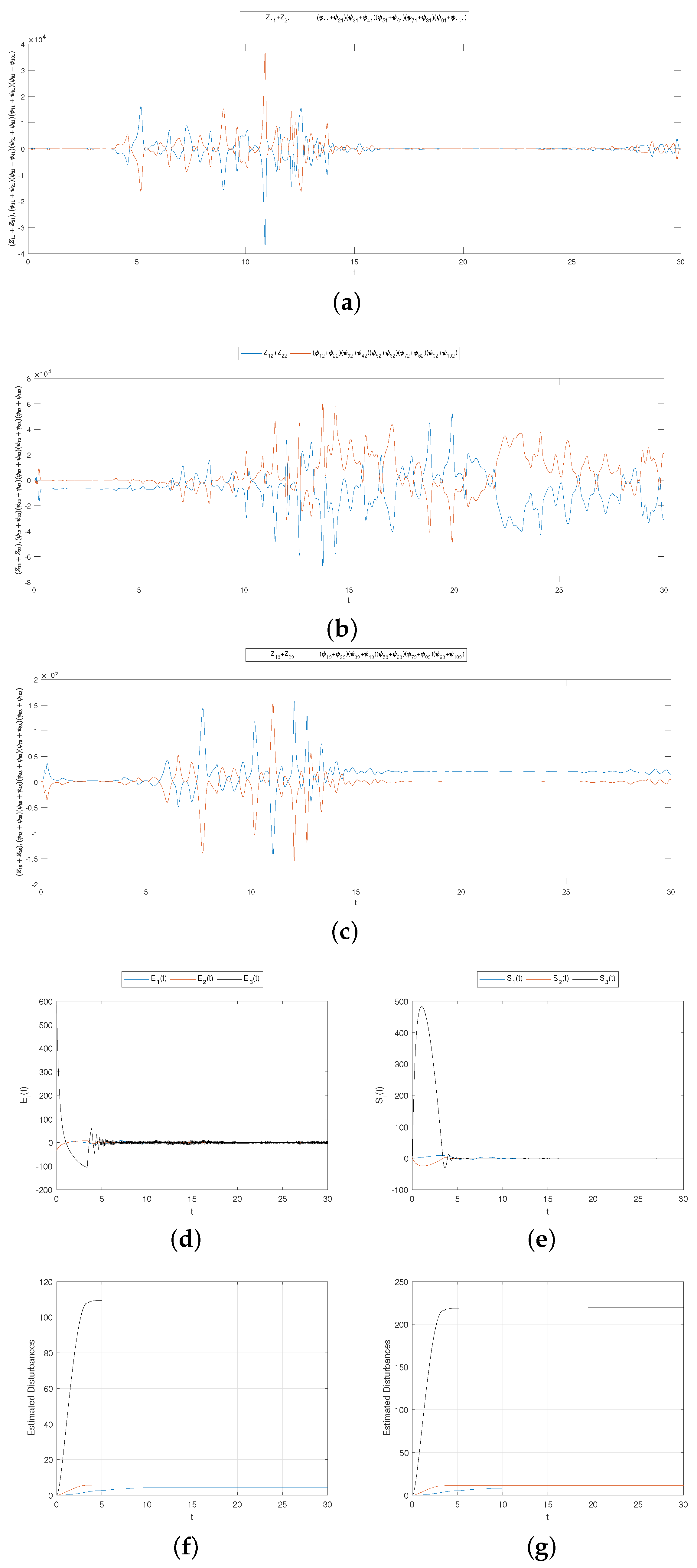
5.2. Via Adaptive Sliding Mode Control

Take $|△H_i|\le A_i$ and $|D_i|\le B_i$. Here, $A_i,B_i>0$ are constants and ${\widehat{A}}_i,\widehat{B_i}$ are estimates $A_i,B_i$.

Consider the sliding surface:

$$S_i\left(t\right)=D^{q-1}{E}_i\left(t\right)+k_i{\int }_0^t{E}_i\left(\xi \right)d\xi .$$

(29)

For (27) at (29), the condition is:

$$S_i\left(t\right)=0,\dot{S_i}\left(t\right)=0.$$

(30)

Differentiating (29):

$$\dot{S_i}\left(t\right)=D^q{E}_i\left(t\right)+k_i{E}_i\left(t\right).$$

(31)

From (30):

$$D^q{E}_i\left(t\right)=-k_i{E}_i\left(t\right).$$

(32)

From Matignon’s theorem [28], (32) is stable. Designing controllers from (28), (32), and SMC theory:

$$\begin{array}{cc}\hfill \overline{U_1}& =-Z_{12}-Z_{13}+5sin\left(Z_{12}\right)-(121{\psi }_{12}-5{\psi }_{11}+83.6{\psi }_{22}-83.6{\psi }_{23}-10{\psi }_{21})({\psi }_{31}+{\psi }_{41})\hfill \\ & ({\psi }_{51}+{\psi }_{61})({\psi }_{71}+{\psi }_{81})({\psi }_{91}+{\psi }_{101})-({\psi }_{11}+{\psi }_{21})({\psi }_{31}+{\psi }_{41})(35{\psi }_{51}-35{\psi }_{51}+-{\psi }_{62}-{\psi }_{63})\hfill \\ & ({\psi }_{71}+{\psi }_{81})({\psi }_{91}+{\psi }_{101})-({\psi }_{11}+{\psi }_{21})({\psi }_{31}+{\psi }_{41})({\psi }_{51}+{\psi }_{61})({\psi }_{71}+{\psi }_{81})(0.7{\psi }_{91}-3{\psi }_{92}{\psi }_{93}\hfill \\ & +0.7{\psi }_{101}-4{\psi }_{102}{\psi }_{103}).\hfill \end{array}$$

(33)

$$\begin{array}{cc}\hfill \overline{U_2}& =Z_{11}-Z_{13}-({\psi }_{11}{\psi }_{13}-{\psi }_{12}+{\psi }_{11}+{\psi }_{21}{\psi }_{23}-{\psi }_{22}+12{\psi }_{12})({\psi }_{32}+{\psi }_{42})({\psi }_{52}+{\psi }_{62})({\psi }_{72}\hfill \\ & +{\psi }_{82})({\psi }_{92}+{\psi }_{102})-({\psi }_{12}+{\psi }_{22})({\psi }_{32}+{\psi }_{42})(-7{\psi }_{51}-{\psi }_{51}{\psi }_{53}+28{\psi }_{52}+{\psi }_{61}+0.4{\psi }_{62})({\psi }_{72}\hfill \\ & +{\psi }_{82})({\psi }_{92}+{\psi }_{102})-({\psi }_{12}+{\psi }_{22})({\psi }_{32}+{\psi }_{42})({\psi }_{52}+{\psi }_{62})({\psi }_{72}+{\psi }_{82})(-0.1{\psi }_{92}+3{\psi }_{91}{\psi }_{93}\hfill \\ & -0.1{\psi }_{102}+4{\psi }_{101}{\psi }_{103}).\hfill \\ \hfill \overline{U_3}& =Z_{11}+Z_{13}-5sin\left(Z_{11}\right)-(-{\psi }_{11}{\psi }_{12}-{\psi }_{13}+-{\psi }_{21}{\psi }_{22}-12{\psi }_{21}-{\psi }_{23})({\psi }_{33}+{\psi }_{43})({\psi }_{53}+{\psi }_{63})\hfill \\ & ({\psi }_{73}+{\psi }_{83})({\psi }_{93}+{\psi }_{103})-({\psi }_{13}+{\psi }_{23})({\psi }_{33}+{\psi }_{43})({\psi }_{51}{\psi }_{52}-3{\psi }_{53}+0.2+{\psi }_{63}({\psi }_{61}-10))\hfill \\ & ({\psi }_{73}+{\psi }_{83})({\psi }_{93}+{\psi }_{103})-({\psi }_{13}+{\psi }_{23})({\psi }_{33}+{\psi }_{43})({\psi }_{53}+{\psi }_{63})({\psi }_{73}+{\psi }_{83})(-0.001-{\psi }_{93}\hfill \\ & +3{\psi }_{91}{\psi }_{92}+0.3{\psi }_{93}{\psi }_{92}-0.001-{\psi }_{103}+4{\psi }_{101}{\psi }_{102}+0.4{\psi }_{103}{\psi }_{102}).\hfill \\ \hfill \overline{U_4}& =-Z_{22}-Z_{23}+5sin\left(Z_{22}\right)-7sin\left(t\right)-({\psi }_{11}+{\psi }_{21})(-2{\psi }_{31}+{\psi }_{32}{\psi }_{33}+10{\psi }_{42}-10{\psi }_{41})({\psi }_{51}\hfill \\ & +{\psi }_{61})({\psi }_{71}+{\psi }_{81})({\psi }_{91}+{\psi }_{101})-({\psi }_{11}+{\psi }_{21})({\psi }_{31}+{\psi }_{41})({\psi }_{51}+{\psi }_{61})(0.7{\psi }_{71}-{\psi }_{72}{\psi }_{73}\hfill \\ & +0.7{\psi }_{81}-2{\psi }_{82}{\psi }_{83})({\psi }_{91}+{\psi }_{101})-E_1-(a_1+b_1+c_1)sign\left(S_1\right).\hfill \\ \hfill \overline{U_5}& =Z_{21}-Z_{23}-sin\left(7t\right)-({\psi }_{12}+{\psi }_{22})(-2{\psi }_{32}+{\psi }_{33}{\psi }_{31}-5{\psi }_{31}+28{\psi }_{41}-{\psi }_{42}-{\psi }_{41}{\psi }_{43})({\psi }_{52}\hfill \\ & +{\psi }_{62})({\psi }_{72}+{\psi }_{82})({\psi }_{92}+{\psi }_{102})-({\psi }_{12}+{\psi }_{22})({\psi }_{32}+{\psi }_{42})({\psi }_{52}+{\psi }_{62})(-0.1{\psi }_{72}+{\psi }_{71}\hfill \\ & {\psi }_{73}-0.1{\psi }_{82}+2{\psi }_{81}{\psi }_{83})({\psi }_{92}+{\psi }_{102})-2E_2-(a_2+b_2+c_2)sign\left(S_2\right).\hfill \\ \hfill \overline{U_6}& =Z_{21}+Z_{23}-5sin\left(Z_{21}\right)-cos\left(Z_{21}\right)-({\psi }_{13}+{\psi }_{23})(1-{\psi }_{31}{\psi }_{32}+\frac{8}{3}{\psi }_{43}+{\psi }_{41}{\psi }_{42})({\psi }_{53}+{\psi }_{63})\hfill \\ & ({\psi }_{73}+{\psi }_{83})({\psi }_{93}+{\psi }_{103})-({\psi }_{13}+{\psi }_{23})({\psi }_{33}+{\psi }_{43})({\psi }_{53}+{\psi }_{63})(-0.001-{\psi }_{73}+{\psi }_{71}{\psi }_{72}+\hfill \\ & 0.1{\psi }_{73}{\psi }_{72}-0.001-{\psi }_{83}+2{\psi }_{81}{\psi }_{82}+0.2{\psi }_{83}{\psi }_{82})({\psi }_{93}+{\psi }_{103})-3E_3-(a_3+b_3+c_3)sign\left(S_3\right).\hfill \\ \hfill \overline{V_1}& =-Z_{32}-Z_{33}+5sin\left(Z_{32}\right)-(121{\psi }_{112}-5{\psi }_{111}+83.6{\psi }_{122}-83.6{\psi }_{123}-10{\psi }_{121})({\psi }_{131}+{\psi }_{141})\hfill \\ & ({\psi }_{151}+{\psi }_{161})({\psi }_{171}+{\psi }_{181})({\psi }_{191}+{\psi }_{201})-({\psi }_{111}+{\psi }_{121})({\psi }_{131}+{\psi }_{141})(35{\psi }_{151}-35{\psi }_{151}-{\psi }_{162}\hfill \\ & -{\psi }_{163})({\psi }_{171}+{\psi }_{181})({\psi }_{191}+{\psi }_{201})-({\psi }_{111}+{\psi }_{121})({\psi }_{131}+{\psi }_{141})({\psi }_{151}+{\psi }_{161})({\psi }_{171}+{\psi }_{181})\hfill \\ & (0.7{\psi }_{191}-3{\psi }_{192}{\psi }_{193}+0.7{\psi }_{201}-4{\psi }_{202}{\psi }_{203}).\hfill \\ \hfill \overline{V_2}& =Z_{31}-Z_{33}-({\psi }_{111}{\psi }_{113}-{\psi }_{112}+{\psi }_{111}+{\psi }_{121}{\psi }_{123}-{\psi }_{122}+12{\psi }_{112})({\psi }_{132}+{\psi }_{142})({\psi }_{152}\hfill \\ & +{\psi }_{162})({\psi }_{172}+{\psi }_{182})({\psi }_{192}+{\psi }_{202})-({\psi }_{112}+{\psi }_{122})({\psi }_{132}+{\psi }_{142})(-7{\psi }_{151}-{\psi }_{151}{\psi }_{153}+28{\psi }_{152}\hfill \\ & +{\psi }_{161}+0.4{\psi }_{162})({\psi }_{172}+{\psi }_{182})({\psi }_{192}+{\psi }_{202})-({\psi }_{112}+{\psi }_{122})({\psi }_{132}+{\psi }_{142})({\psi }_{152}+{\psi }_{162})({\psi }_{172}\hfill \\ & +{\psi }_{182})(-0.1{\psi }_{192}+3{\psi }_{191}{\psi }_{193}-0.1{\psi }_{202}+4{\psi }_{201}{\psi }_{203}).\hfill \\ \hfill \overline{V_3}& =Z_{31}+Z_{33}-5sin\left(Z_{11}\right)-(-{\psi }_{111}{\psi }_{112}-{\psi }_{113}+-{\psi }_{121}{\psi }_{122}-12{\psi }_{121}-{\psi }_{123})({\psi }_{133}+{\psi }_{143})\hfill \\ & ({\psi }_{153}+{\psi }_{163})({\psi }_{173}+{\psi }_{183})({\psi }_{193}+{\psi }_{203})-({\psi }_{113}+{\psi }_{123})({\psi }_{133}+{\psi }_{143})({\psi }_{151}{\psi }_{152}-3{\psi }_{153}\hfill \\ & +0.2+{\psi }_{163}({\psi }_{161}-10))({\psi }_{173}+{\psi }_{183})({\psi }_{193}+{\psi }_{203})-({\psi }_{113}+{\psi }_{123})({\psi }_{133}+{\psi }_{143})({\psi }_{153}\hfill \\ & +{\psi }_{163}\left)({\psi }_{173}+{\psi }_{183})\right(-0.001-{\psi }_{193}+3{\psi }_{191}{\psi }_{192}+0.3{\psi }_{193}{W}_{192}-0.001-{\psi }_{203}\hfill \\ & +4{\psi }_{201}{\psi }_{202}+0.4{\psi }_{203}{\psi }_{202}).\hfill \\ \hfill \overline{V_4}& =-Z_{42}-Z_{43}+5sin\left(Z_{42}\right)-7sin\left(t\right)-({\psi }_{111}+{\psi }_{121})(-2{\psi }_{131}+{\psi }_{132}{\psi }_{133}+10{\psi }_{142}-10{\psi }_{141})\hfill \\ & ({\psi }_{151}+{\psi }_{161})({\psi }_{171}+{\psi }_{181})({\psi }_{191}+{\psi }_{201})-({\psi }_{111}+{\psi }_{121})({\psi }_{131}+{\psi }_{141})({\psi }_{151}+{\psi }_{161})\hfill \\ & (0.7{\psi }_{171}-{\psi }_{172}{\psi }_{173}+0.7{\psi }_{181}-2{\psi }_{182}{\psi }_{183})({\psi }_{191}+{\psi }_{201})-E_4-(a_4+b_4+c_4)sign\left(S_4\right).\hfill \\ \hfill \overline{V_5}& =Z_{41}-Z_{43}-sin\left(7t\right)-({\psi }_{112}+{\psi }_{122})(-2{\psi }_{132}+{\psi }_{133}{\psi }_{131}-5{\psi }_{131}+28{\psi }_{141}-{\psi }_{142}\hfill \\ & -{\psi }_{141}{\psi }_{143})({\psi }_{152}+{\psi }_{162})({\psi }_{172}+{\psi }_{182})({\psi }_{192}+{\psi }_{202})-({\psi }_{112}+{\psi }_{122})({\psi }_{132}+{\psi }_{142})({\psi }_{152}+{\psi }_{162})\hfill \\ & (-0.1{\psi }_{172}+{\psi }_{171}{\psi }_{173}-0.1{\psi }_{182}+2{\psi }_{181}{\psi }_{183})({\psi }_{192}+{\psi }_{202})-2E_5-(a_5+b_5+c_5)sign\left(S_5\right).\hfill \\ \hfill \overline{V_6}& =Z_{41}+Z_{43}-5sin\left(Z_{41}\right)-cos\left(Z_{41}\right)-({\psi }_{113}+{\psi }_{123})(1-{\psi }_{131}{\psi }_{132}+\frac{8}{3}{\psi }_{143}+{\psi }_{141}{\psi }_{142})({\psi }_{153}\hfill \\ & +{\psi }_{163})({\psi }_{173}+{\psi }_{183})({\psi }_{193}+{\psi }_{203})-({\psi }_{113}+{\psi }_{123})({\psi }_{133}+{\psi }_{143})({\psi }_{153}+{\psi }_{163})(-0.001\hfill \\ & -{\psi }_{173}+{\psi }_{171}{\psi }_{172}+0.1{\psi }_{173}{\psi }_{172}-0.001-{\psi }_{183}+2{\psi }_{181}{\psi }_{182}+0.2{\psi }_{183}{\psi }_{182})({\psi }_{193}+{\psi }_{203})\hfill \\ & -3E_6-(a_6+b_6+c_6)sign\left(S_6\right).\hfill \end{array}$$

where $sign(.)$ is the signum function and $c_i>0$ are constants.

Update the parameters as:

$$\begin{array}{c}\hfill {\dot{\widehat{A}}}_i=a_i\mid S_i\mid .\\ \hfill {\dot{\widehat{B}}}_i=b_i\mid S_i\mid .\end{array}$$

(34)

for positive $a_i,b_i$.

Theorem 1.

Fractional Disturbed Master Systems (2)–(5) and Slave Systems (6)–(25) will achieve stability and synchronization using controllers and parameter updates as in (33)–(34).

Proof. 

Stability using Lyapunov’s direct method [29] is proven considering positive definite function V and the negative derivative proving error convergence to zero.

Let:

$$V=\sum _{i=1}^6{V}_i.$$

(35)

where:

$$\begin{array}{c}\hfill V_1={\displaystyle \frac{1}{2}}{S}_1^2+{\displaystyle \frac{1}{2a_1}}{({\widehat{A}}_1-A_1)}^2+{\displaystyle \frac{1}{2b_1}}{({\widehat{B}}_1-B_1)}^2.\\ \hfill V_2={\displaystyle \frac{1}{2}}{S}_2^2+{\displaystyle \frac{1}{2a_2}}{({\widehat{A}}_2-A_2)}^2+{\displaystyle \frac{1}{2b_2}}{({\widehat{B}}_2-B_2)}^2.\\ \hfill V_3={\displaystyle \frac{1}{2}}{S}_3^2+{\displaystyle \frac{1}{2a_3}}{({\widehat{A}}_3-A_3)}^2+{\displaystyle \frac{1}{2b_3}}{({\widehat{B}}_3-B_3)}^2.\\ \hfill V_4={\displaystyle \frac{1}{2}}{S}_4^2+{\displaystyle \frac{1}{2a_4}}{({\widehat{A}}_4-A_4)}^2+{\displaystyle \frac{1}{2b_4}}{({\widehat{B}}_4-B_4)}^2.\\ \hfill V_5={\displaystyle \frac{1}{2}}{S}_5^2+{\displaystyle \frac{1}{2a_5}}{({\widehat{A}}_5-A_5)}^2+{\displaystyle \frac{1}{2b_5}}{({\widehat{B}}_5-B_5)}^2.\\ \hfill V_6={\displaystyle \frac{1}{2}}{S}_6^2+{\displaystyle \frac{1}{2a_6}}{({\widehat{A}}_6-A_6)}^2+{\displaystyle \frac{1}{2b_6}}{({\widehat{B}}_6-B_6)}^2.\end{array}$$

(36)

Differentiating:

$$\begin{array}{c}\hfill {\dot{V}}_1=S_1\dot{S_1}+{\displaystyle \frac{1}{a_1}}({\widehat{A}}_1-A_1){\dot{\widehat{A}}}_1+{\displaystyle \frac{1}{b_1}}({\widehat{B}}_1-B_1){\dot{\widehat{B}}}_1.\\ \hfill {\dot{V}}_2=S_2\dot{S_2}+{\displaystyle \frac{1}{a_2}}({\widehat{A}}_2-A_2){\dot{\widehat{A}}}_2+{\displaystyle \frac{1}{b_2}}({\widehat{B}}_2-B_2){\dot{\widehat{B}}}_2.\\ \hfill {\dot{V}}_3=S_3\dot{S_3}+{\displaystyle \frac{1}{a_3}}({\widehat{A}}_3-A_3){\dot{\widehat{A}}}_3+{\displaystyle \frac{1}{b_3}}({\widehat{B}}_3-B_3){\dot{\widehat{B}}}_3.\\ \hfill {\dot{V}}_4=S_4\dot{S_4}+{\displaystyle \frac{1}{a_4}}({\widehat{A}}_4-A_4){\dot{\widehat{A}}}_4+{\displaystyle \frac{1}{b_4}}({\widehat{B}}_4-B_4){\dot{\widehat{B}}}_4.\\ \hfill {\dot{V}}_5=S_5\dot{S_5}+{\displaystyle \frac{1}{a_5}}({\widehat{A}}_5-A_5){\dot{\widehat{A}}}_5+{\displaystyle \frac{1}{b_5}}({\widehat{B}}_5-B_5){\dot{\widehat{B}}}_5.\\ \hfill {\dot{V}}_6=S_6\dot{S_6}+{\displaystyle \frac{1}{a_6}}({\widehat{A}}_6-A_6){\dot{\widehat{A}}}_6+{\displaystyle \frac{1}{b_6}}({\widehat{B}}_6-B_6){\dot{\widehat{B}}}_6.\end{array}$$

(37)

From (31), we have:

$$\begin{array}{c}\hfill {\dot{V}}_1=S_1(D^q{E}_1+k_1{E}_1)+{\displaystyle \frac{1}{a_1}}({\widehat{A}}_1-A_1){\dot{\widehat{A}}}_1+{\displaystyle \frac{1}{b_1}}({\widehat{B}}_1-B_1){\dot{\widehat{B}}}_1.\\ \hfill {\dot{V}}_2=S_2(D^q{E}_2+k_2{E}_2)+{\displaystyle \frac{1}{a_2}}({\widehat{A}}_2-A_2){\dot{\widehat{A}}}_2+{\displaystyle \frac{1}{b_2}}({\widehat{B}}_2-B_2){\dot{\widehat{B}}}_2.\\ \hfill {\dot{V}}_3=S_3(D^q{E}_3+k_3{E}_3)+{\displaystyle \frac{1}{a_3}}({\widehat{A}}_3-A_3){\dot{\widehat{A}}}_3+{\displaystyle \frac{1}{b_3}}({\widehat{B}}_3-B_3){\dot{\widehat{B}}}_3.\\ \hfill {\dot{V}}_4=S_4(D^q{E}_4+k_4{E}_4)+{\displaystyle \frac{1}{a_4}}({\widehat{A}}_4-A_4){\dot{\widehat{A}}}_4+{\displaystyle \frac{1}{b_4}}({\widehat{B}}_4-B_4){\dot{\widehat{B}}}_4.\\ \hfill {\dot{V}}_5=S_5(D^q{E}_5+k_5{E}_5)+{\displaystyle \frac{1}{a_5}}({\widehat{A}}_5-A_5){\dot{\widehat{A}}}_5+{\displaystyle \frac{1}{b_5}}({\widehat{B}}_5-B_5){\dot{\widehat{B}}}_5.\\ \hfill {\dot{V}}_6=S_6(D^q{E}_6+k_6{E}_6)+{\displaystyle \frac{1}{a_6}}({\widehat{A}}_6-A_6){\dot{\widehat{A}}}_6+{\displaystyle \frac{1}{b_6}}({\widehat{B}}_6-B_6){\dot{\widehat{B}}}_6.\end{array}$$

(38)

Substituting the values in Equation (38):

$$\begin{array}{cc}\hfill {\dot{V}}_i& =S_1[-△H_i-D_i({\widehat{A}}_i+{\widehat{B}}_i+r_i)sign{S}_i]+({\widehat{A}}_i-A_i)\left|S_i\right|+({\widehat{B}}_i-B_i)\left|S_i\right|.\hfill \\ \hfill & \le (|△H_i|+\left|D_i\right|)\left|S_i\right|+({\widehat{A}}_i-A_i)\left|S_i\right|+({\widehat{B}}_i-B_i)\left|S_i\right|.\hfill \\ \hfill & <(A_i+B_i)\left|S_i\right|-({\widehat{A}}_i+{\widehat{B}}_i+r_i)\left|sign{S}_i\right|+({\widehat{A}}_i-A_i)\left|S_i\right|+({\widehat{B}}_i-B_i)\left|S_i\right|.\hfill \\ \hfill & =-t_i\left|S_i\right|.\hfill \end{array}$$

Therefore:

$$\begin{array}{cc}\hfill \dot{V}& =\sum _{i=1}^6{\dot{V}}_i.\hfill \\ \hfill & <-\sum _{i=1}^6\left(t_i\left|S_i\right|\right).\hfill \end{array}$$

(39)

Now ∃ at $\ge 0\in R$ such that:

$$\sum _{i=1}^6{t}_i\left|S_i\right|>t.$$

then:

$$\begin{array}{cc}\hfill \dot{V}& <-t\sqrt{S_1^2+S_2^2+S_3^2+S_4^2+S_5^2+S_6^2}.\hfill \\ \hfill & <0.\hfill \end{array}$$

(40)

□

From the Lyapunov stability theory, errors converge to $S_i=0$.

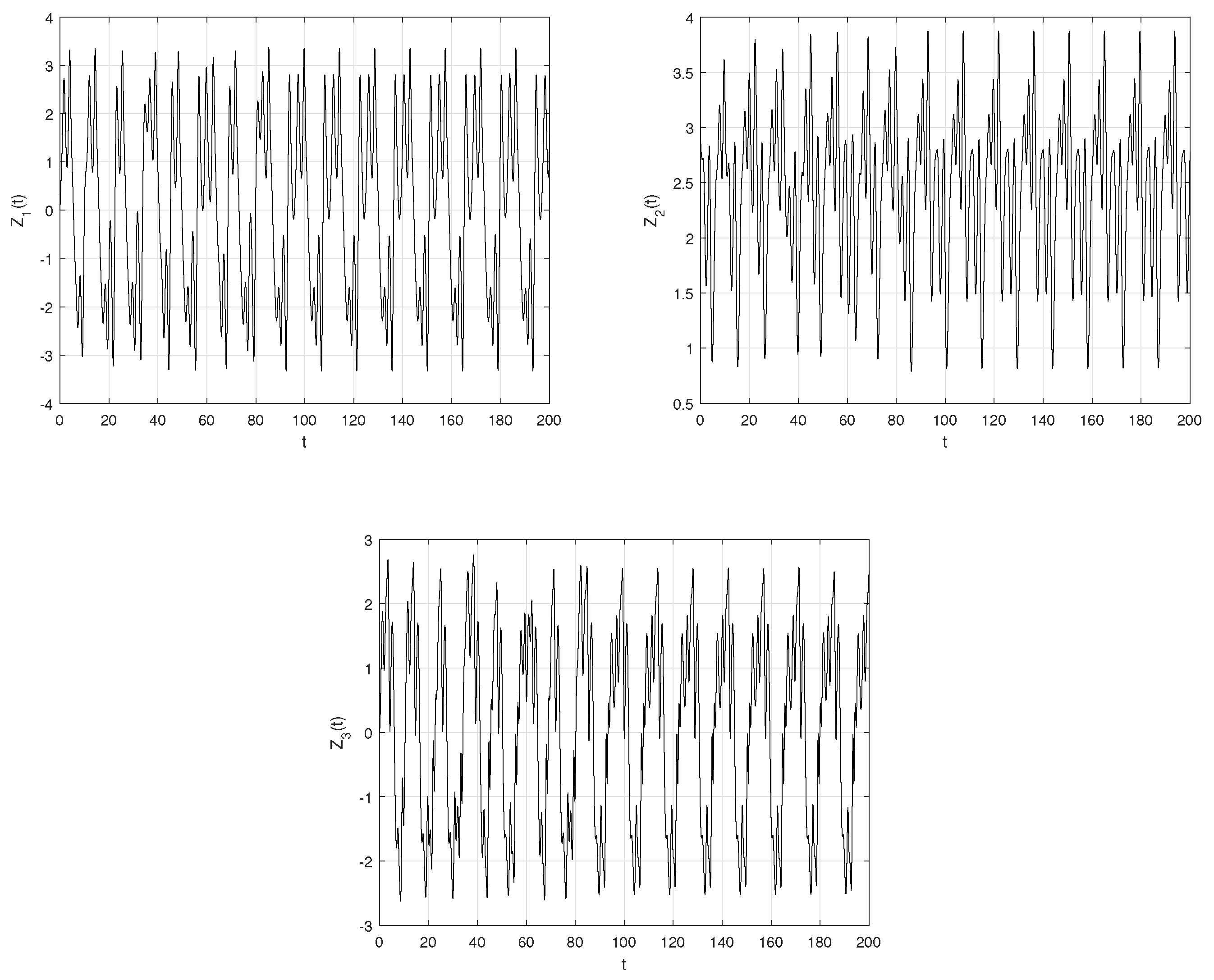
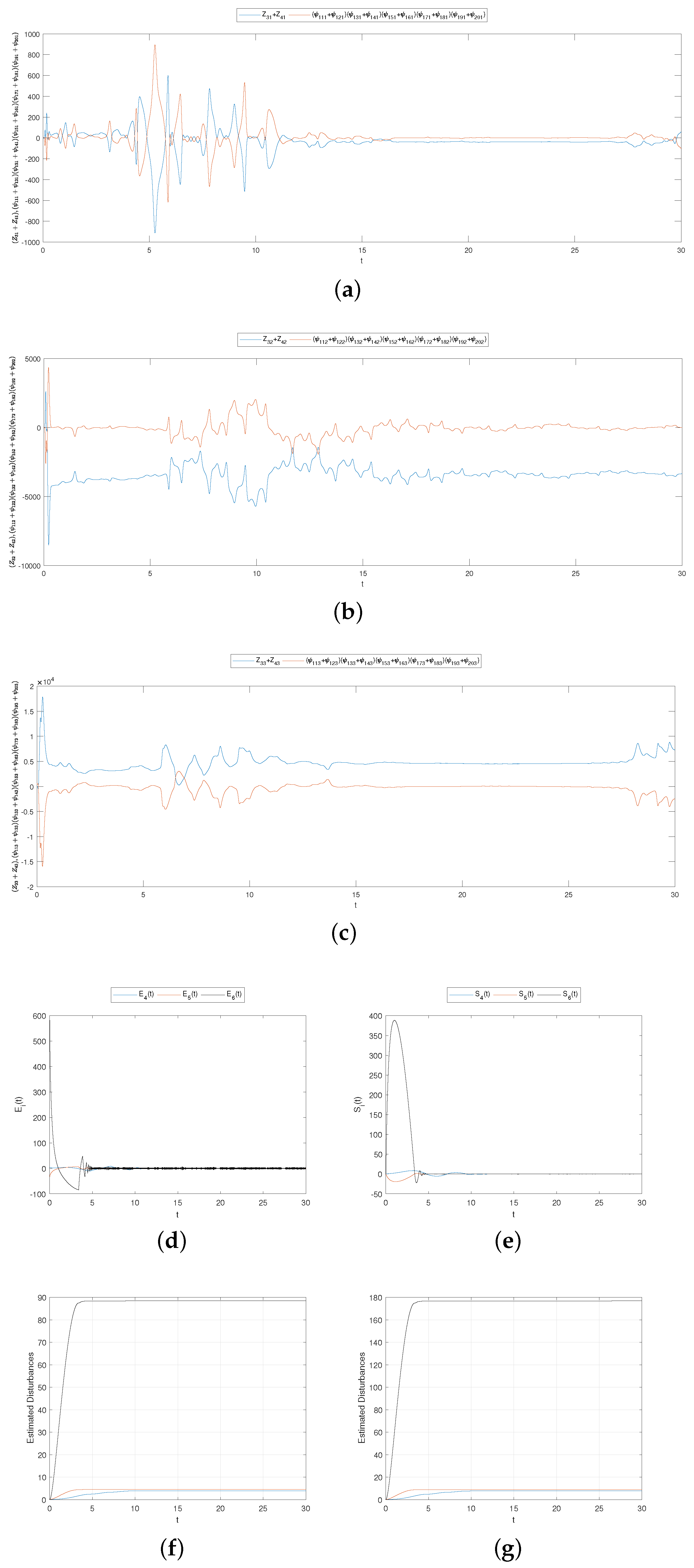
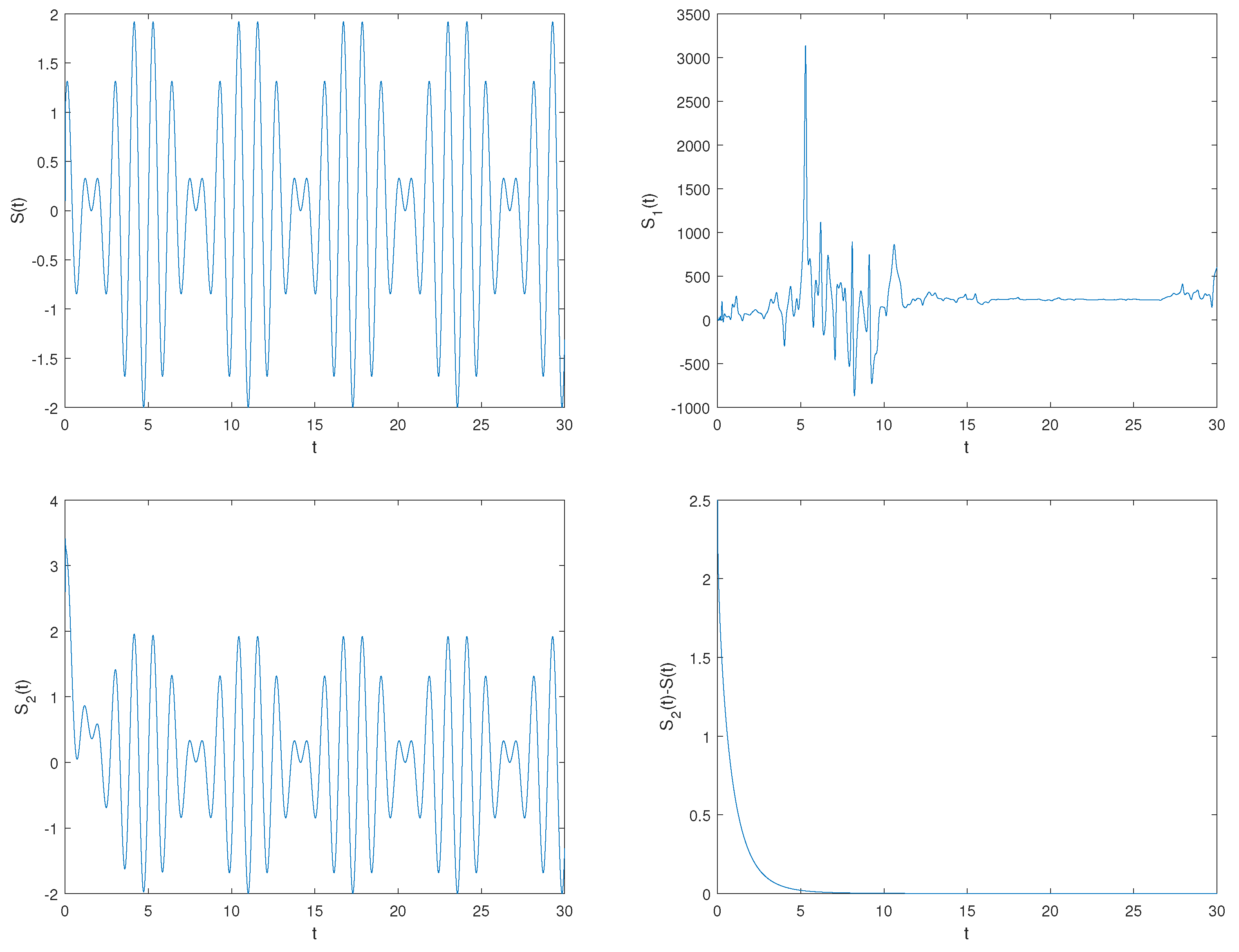
5.3. Simulations and Proposed Application

The dual penta-compound combination anti-synchronized trajectories and error using the non-linear control method are displayed in Figure 7. The synchronized trajectories using the adaptive SMC technique are displayed in Figure 8a–c and Figure 9a–c. Figure 8d and Figure 9d show the anti-synchronization error using the SMC technique. The sliding surfaces tending to zero are shown in Figure 8e and Figure 9e. The disturbances and uncertainties $△H_1=0,D_1=7sin\left(t\right),△H_2=0,D_2=sin\left(7t\right),△H_3=cos\left(Z_{21}\right),D_3=0,△H_4=0,D_4=7sin\left(t\right),△H_5=0,D_5=sin\left(7t\right),△H_6=cos\left(Z_{21}\right),D_6=0$ are estimated and shown in Figure 8f,g and Figure 9f,g by estimating the parameters using I.C. as $\widehat{A_i}=\widehat{B_i}=0.1$ and $c_1=1,c_2=2,c_3=3$, $c_4=1,c_5=2,c_6=3$, respectively.

The achieved anti-synchronization is illustrated with an example for application in secure communication. In this synchronization, we have two pairs of penta-compound combinations from which to choose. This adds to the diversity in the options for encrypting the original message. The sum of the chaotic signals from the master systems is added to the original signal; the encrypted signal is formed and transmitted. At the receiving end, upon performing synchronization, the controllers are applied and decrypted.

Suppose $S\left(t\right)=sin\left(5t\right)+cos\left(6t\right)$ as the original signal. Mix $S\left(t\right)$ with chaotic signals $Z_{11}+Z_{21}$ to obtain $S_1\left(t\right)$. Apply controllers to recover $S_2\left(t\right)$ at the receiver, as illustrated in Figure 10.

6. Conclusions

In this paper, dual penta-compound combination anti-synchronization was performed on a chaotic system with two sine non-linearities. A thorough analysis of the newly introduced fractional-order system was performed. The achieved synchronization was performed between four master systems and twenty slave systems using two techniques. Uncertainties and disturbances were estimated. An application in secure communication was illustrated with the help of an example.

Studying the hidden attractors of the system and its electronic circuit implementation are the future scope.

References

1. Javidi, M.; Nyamoradi, N. Dynamic analysis of a fractional order prey-predator interaction with harvesting. Appl. Math. Model. 2013, 37, 28946–28956. [Google Scholar] [CrossRef]
2. Baleanu, D.; Jajarmi, A.; Mohammadi, H.; Rezapour, S. A new study on the mathematical modelling of human liver with Caputo–Fabrizio fractional derivative. Chaos Solitons Fractals 2020, 134, 109705. [Google Scholar] [CrossRef]
3. Baleanu, D.; Jajarmi, A.; Sajjadi, S.S.; Asad, J.H. The fractional features of a harmonic oscillator with position-dependent mass. In Communications in Theoretical Physics; IOP Publishing: Philadelphia, PA, USA, 2020; Volume 72. [Google Scholar]
4. Baleanu, D.; Etemad, S.; Rezapour, S. A hybrid Caputo fractional modeling for thermostat with hybrid boundary value conditions. Bound. Value Probl. 2020, 64, 1–16. [Google Scholar] [CrossRef] [Green Version]
5. Khan, A.; Trikha, P. Study of earths changing polarity using compound difference synchronization. GEM Int. J. Geomath. 2020, 11, 7. [Google Scholar] [CrossRef] [Green Version]
6. Khan, A.; Trikha, P.; Lone, S.J. Secure Communication: Using synchronization on a novel fractional-order chaotic system. In Proceedings of the ICPECA, New Delhi, India, 16–17 November 2019. [Google Scholar]
7. Sun, S. A novel hyperchaotic image encryption scheme based on dna encoding, pixel-level scrambling and bit-level scrambling. IEEE Photonics J. 2018, 10, 1–14. [Google Scholar] [CrossRef]
8. Trikha, P.; Jahanzaib, L.S. Dynamical analysis of a novel 5-d hyper-chaotic system with no equilibrium point and its application in secure communication. Differ. Geom. Dyn. Syst. 2020, 22, 269–288. [Google Scholar]
9. Zhang, S.; Zeng, Y.; Li, Z. One to four-wing chaotic attractors coined from a novel 3d fractional-order chaotic system with complex dynamics. Chin. J. Phys. 2018, 56, 793–806. [Google Scholar] [CrossRef]
10. Wang, Z.; Sun, Y.; Cang, S. A 3-D Spherical Attractor. Acta Phys. Polonica Ser. B 2011, B42, 235–247. [Google Scholar] [CrossRef]
11. Yu, S.; Lu, J.; Chen, G. Multifolded torus chaotic attractors: Design and implementation. Chaos: Interdiscip. J. Nonlinear Sci. 2007, 17, 013118. [Google Scholar] [CrossRef] [Green Version]
12. Chua, L.; Komuro, M.; Matsumoto, T. The double scroll family. IEEE Trans. Circuits Syst. 1986, 33, 1072–1118. [Google Scholar] [CrossRef] [Green Version]
13. Pecora, L.M.; Carroll, T.L. Synchronization in chaotic systems. Phys. Rev. Lett. 1990, 64, 821. [Google Scholar] [CrossRef]
14. Trikha, P.; Jahanzaib, L.S. Secure Communication: Using Double Compound-Combination Hybrid Synchronization. In Proceedings of the International Conference on Artificial Intelligence and Applications; Springer: Singapore, 2021; pp. 81–91. [Google Scholar]
15. Khan, A.; Trikha, P. Compound difference anti-synchronization between chaotic systems of integer and fractional order. SN Appl. Sci. 2019, 1, 757. [Google Scholar] [CrossRef] [Green Version]
16. Rosenblum, M.G.; Pikovsky, A.S.; Kurths, J. From phase to lag synchronization in coupled chaotic oscillators. Phys. Rev. E 1997, 78, 4193. [Google Scholar] [CrossRef]
17. Runzi, L.; Yinglan, W.; Shucheng, D. Combination synchronization of three classic chaotic systems using active backstepping design. Chaos: Interdiscip. J. Nonlinear Sci. 2011, 21, 043114. [Google Scholar] [CrossRef]
18. Khan, A.; Jahanzaib, L.S.; Trikha, P. Secure Communication: Using Parallel Synchronization Technique On Novel Fractional Order Chaotic System. IFAC-PapersOnLine 2020, 53, 307–312. [Google Scholar] [CrossRef]
19. Khan, A.; Trikha, P.; Jahanzaib, L.S. Dislocated hybrid synchronization via. tracking control & parameter estimation methods with application. Int. J. Model. Simul. 2020, 41, 415–425. [Google Scholar] [CrossRef]
20. Khan, A.; Jahanzaib, L.S.; Trikha, P. Fractional Inverse Matrix Projective Combination Synchronization with Application in Secure Communication. In Proceedings of the International Conference on Artificial Intelligence and Applications; Springer: Singapore, 2021; pp. 93–101. [Google Scholar]
21. Mahmoud, E.E.; Jahanzaib, L.S.; Trikha, P.; Alkinani, M.H. Anti-synchronized quad-compound combination among parallel systems of fractional chaotic system with application. Alex. Eng. J. 2020, 59, 4183–4200. [Google Scholar] [CrossRef]
22. Sun, J.; Li, N.; Fang, J. Combination-combination projective synchronization of multiple chaotic systems using sliding mode control. Adv. Math. Phys. 2018, 2018, 2031942. [Google Scholar] [CrossRef] [Green Version]
23. Sun, J.; Shen, Y.; Yin, Q.; Xu, C. Compound synchronization of four memristor chaotic oscillator systems and secure communication. Chaos: Interdiscip. J. Nonlinear Sci. 2013, 23, 140. [Google Scholar] [CrossRef]
24. Sun, J.; Wang, Y.; Cui, G.; Shen, Y. Compound-combination synchronization of five chaotic systems via nonlinear control. Int. J. Light Electron. Opt. 2016, 127, 4136–4143. [Google Scholar] [CrossRef]
25. Khan, A.; Lone, S.J.; Trikha, P. Analysis of a Novel 3-D Fractional Order Chaotic System. In Proceedings of the ICPECA, New Delhi, India, 16–17 November 2019. [Google Scholar]
26. Geist, K.; Parlitz, U.; Lauterborn, W. Comparison of different methods for computing lyapunov exponents. Prog. Theor. Phys. 1990, 83, 875–893. [Google Scholar] [CrossRef]
27. Tavassoli, M.H.; Tavassoli, A.; Rahimi, M.R.O. The geometric and physical interpretation of fractional-order derivatives of polynomial functions. Differ. Geom. Dyn. Syst. 2013, 15, 93–104. [Google Scholar]
28. Matignon, D. Stability results for fractional differential equations with applications to control processing. In Computational Engineering in Systems Applications; IMACS; IEEE-SMC: Lille, France, 1996; Volume 2, pp. 963–968. [Google Scholar]
29. Vidyasagar, M. Nonlinear Systems Analysis; Society for Industrial and Applied Mathematics: Philadelphia, PA, USA, 2002; Volume 42. [Google Scholar]
Figure 1. State trajectories of (1).
Fractalfract 05 00264 g001
Figure 2. Phase diagrams of (1).
Fractalfract 05 00264 g002
Figure 3. Bifurcation diagram of (1) for (a) 4.75 A 5.25 and (b) 4.75 B 5.25 .
Fractalfract 05 00264 g003
Figure 4. Dynamics of (2) for 0.8 q 1 .
Fractalfract 05 00264 g004
Figure 5. Phase portraits of Master Systems (2)–(5).
Fractalfract 05 00264 g005
Figure 6. Phase portraits of Slave Systems (6)–(25).
Fractalfract 05 00264 g006
Figure 7. Synchronized trajectories and error via the non-linear control method.
Fractalfract 05 00264 g007
Figure 8. (ac) Synchronized trajectories via adaptive sliding mode control. (d) Error. (e) Surface converging to zero. (f,g) Disturbance estimates.
Fractalfract 05 00264 g008
Figure 9. (ac) Synchronized trajectories via adaptive sliding mode control. (d) Error. (e) Surface converging to zero. (f,g) Disturbance estimates.
Fractalfract 05 00264 g009
Figure 10. Proposed application.
Fractalfract 05 00264 g010
Publisher’s Note: MDPI stays neutral with regard to jurisdictional claims in published maps and institutional affiliations.