Power Law Kernel Analysis of MHD Maxwell Fluid with Ramped Boundary Conditions: Transport Phenomena Solutions Based on Special Functions

Abstract

In this paper, a new approach to find exact solutions is carried out for a generalized unsteady magnetohydrodynamic transport of a rate-type fluid near an unbounded upright plate, which is analyzed for ramped-wall temperature and velocity with constant concentration. The vertical plate is suspended in a porous medium and encounters the effects of radiation. An innovative definition of the time-fractional operator in power-law-kernel form is implemented to hypothesize the constitutive mass, energy, and momentum equations. The Laplace integral transformation technique is applied on a dimensionless form of governing partial differential equations by introducing some non-dimensional suitable parameters to establish the exact expressions in terms of special functions for ramped velocity, temperature, and constant-concentration fields. In order to validate the problem, the absence of the mass Grashof parameter led to the investigated solutions obtaining good agreement in existing literature. Additionally, several system parameters were used, such as as magnetic value M, Prandtl value $Pr$, Maxwell parameter $\lambda$, dimensionless time $\tau$, Schmidt number “$Sc$”, fractional parameter $\alpha$, andMass and Thermal Grashof numbers $Gm$ and $Gr$, respectively, to examine their impacts on velocity, wall temperature, and constant concentration. Results are also discussed in detail and demonstrated graphically via Mathcad-15 software. A comprehensive comparative study between fractional and non-fractional models describes that the fractional model elucidate the memory effects more efficiently.

1. Introduction

The study of non-Newtonian fluids is a very interesting topic for many researchers due to its wide applications in modern technologies and many industrial sectors. Non-Newtonian fluids deals with problems related to chemical engineering, polymers, petroleum, paints, pharmaceutical, plastics, and food processing industries. Furthermore, these types of models also represent fluids such as biological materials, ketchup, polymeric liquids, motor oils, personal care products (shampoo, creams, toothpastes), complex mixtures, etc. However, in the literature, different types of fluid models exist, included rate-type, differential, and integral models. However, many researchers have addressed the rate-type fluid model, because from the research point of view, it is more applicable, due to its elastic effects and memory. Therefore, in this present work, rate-type models are recognized as Maxwell models. Further, Maxwell designed this model to estimate air’s viscoelastic characteristics [1]. Furthermore, Jordan et al. [2] studied exact solutions for Stokes problems of the first type, including the Maxwell model. Moreover, Fetecau et al. [3] explored Stokes problems of second type by assuming the flow of fluid placed on a surface of infinite plate that is vacillating on the plane. Further, the model generated by Maxwell is known as an uncomplicated model designed for expecting the rheological performance of fluids, and it has both viscosity and elasticity as features. Fetecau [4] invetigated exact solution for an infinite vertical surface. The effects of thermophorsis and chemically reactive impacts on flow of Maxwell fluids were studied by Noor [5].

There is no denying the fact that when heat is extracted from a high-temperature wall through a fluid with a certain movement, this mechanism is referred to as heat convection (advection). This mechanism involves interactions between molecular diffusion and the motion of the fluid on the basis of natural as well as forced convection. This is because convective heat transfer transpires when the surface temperature varies from that of the encompassing fluid [6]. Solangi et al. [7] interrogated unique heat conduction properties for increasing concentrations. The focus of this work was to discuss the particle size control for heat exchange and mass concentration behavior on fluids. Soomro et al. [8] carried out the typical analysis of a stretching surface to develop the heat transmission for the flow of non-Newtonian nano-fluids. For physical aspects, numerical computation has been invoked to understand the governing equations based on the finite difference schemes that describe heat transfer phenomena. Shafiq et al. [9] explored an interesting study of the magnetohydrodynamic convective flow to explore the transfer rate of heat, motile microorganisms, and mass. They emphasized in their parametric study the problem for Brownian motion, buoyancy forces, thermophoretic, magnetic field, and Newtonian heating for temperature and concentration. Kashif et al. [10] investigated dual thermal analysis to understand the role of temperature dissimilarity versus temperature or time by using the suspension of nanoparticles. The core objective of this study was to highlight the problem through fractional operators and special functions. Heat transmission over the stretching sheet based on the magnetohydrodynamic two-dimensional Casson fluid flow was observed by Hamid et al. [11]. They examined linearly convected heat effects on twofold solutions in which numerical stability was discussed for the dual results from the governing equation of the problem. Abro et al. [12] suggested the fractional study for thermal radiation of Jeffery fluid and reduced the sub-solutions from fluid motion of the second grade with and without magnetic field. The thermal properties of the governing equations have been treated by integral transform approach. Sheikholeslami et al. [13] observed magnetizable hybrid fluid in the core of a circular cavity with two heaters in circular form subjected to carbon nanotubes. Their focus point in this work was to create magnetic strengths in the wires using electrical current. Abdelmalek et al. [14] applied a hybrid technique known as Control Volume Finite Element Scheme to a curvy circular heater with nano-sized particles using convective heat transmission. They suggested the finding and concluded that conformation of the curvy heater played a essential role in managing the heat emission rate and controlling the convectional flow within the enclosure. Kashif [15] applied surface modification technology to analyze the thermo-dissipation effects on time-dependent natural convectional flow of fluid. Finite Fourier sine transform, Laplace, and fractional techniques have been utilized in the governing equations for exhibiting typical and rheological properties of the problem [16,17,18]. Although studies on heat and transfer analysis can be continued, relevant studies can be observed in categorical formats such as heat transfer via analytical approaches [19,20,21,22,23,24,25,26], heat transfer via numerical approaches [27,28,29,30,31,32], heat transfer via fractional calculus approaches [33,34,35,36], and heat transfer via multi-dimensional approaches [37,38,39,40].

Fractional order calculus has been rapidly increasing in popularity these days because of its useful and exclusive features that are absent in non-fractional calculus. For example, classical models are unable to predict the earlier state of the process known as the memory effect, but fractional calculus is famous for having memory effects. It has been well-known in recent decades for several real-world physical problems that fractional operators are more effective in differentiation compared to integral derivatives. Consequently, in modern times, a generalization of problems from the classical setting to the fractional setting is a subject of concern for many researchers. Generally, most circuit models are explained in terms of fractional differential equations. Therefore, fractional calculus is used in several fields, such as viscoelasticity, economics, relaxation processes, and fluid dynamics. It can be found in the literature that several fractional differential operators exist; for instance, Caputo with kernel (singular and local), Atangana–Baleanu with kernel (non-singular and non-local), Caputo–Fabrizio with kernel (non-singular and local), and a few others have been discussed [41,42,43,44]. For local and non-local kernels, convective flow with ramped conditions of temperature has been studied by Riaz et al. [45]. Furthermore, in a comparative study of MHD Maxwell fluid, the heat effect, with the application of local and non-local operators, is highlighted by Riaz et al. [46]. Some other fractional-associated references have been investigated [47,48,49,50,51], dealing with non-integer differential operators, MHD Jeffrey fluid movement, heat transport, and second-grade fluid. For more details, see [52,53,54,55].

Talha Anwar et al. [56] recently discussed the same problem with a classical approach, but without analyzing the diffusion equation, and executed the approximate result for the proposed problem by using the Laplace transformation technique and Durbin’s numerical algorithm [57]. Based on the aforementioned literature, the object of this exploration is to develop the fractional model by using the modern interpretation of Caputo fractional operator and then derive the exact solution of the considered problem and make the comparison with results obtained by Talha Anwar et al. [56]. The consequences of different related physical parameters are explored, namely thermal Grashof number $Gr$, magnetic field M, dimensionless time $\tau$, fractional parameter $\alpha$, Schmidt number $Sc$, mass Grashof number $Gm$, and Prandtl number $Pr$, on non- dimensional velocity, concentration, and temperature. The results are discussed in detail and demonstrated graphically via Mathcad-15 software. Motivated by the above consideration, the main theme of this manuscript is to show the significance of fractional models corresponding to ordinary existing models for Maxwell fluid. In the end, solutions for some recently published work are compared with the current study, which endorses the authenticity of our solutions and proves that those investigations are limiting or special cases of the current problem.

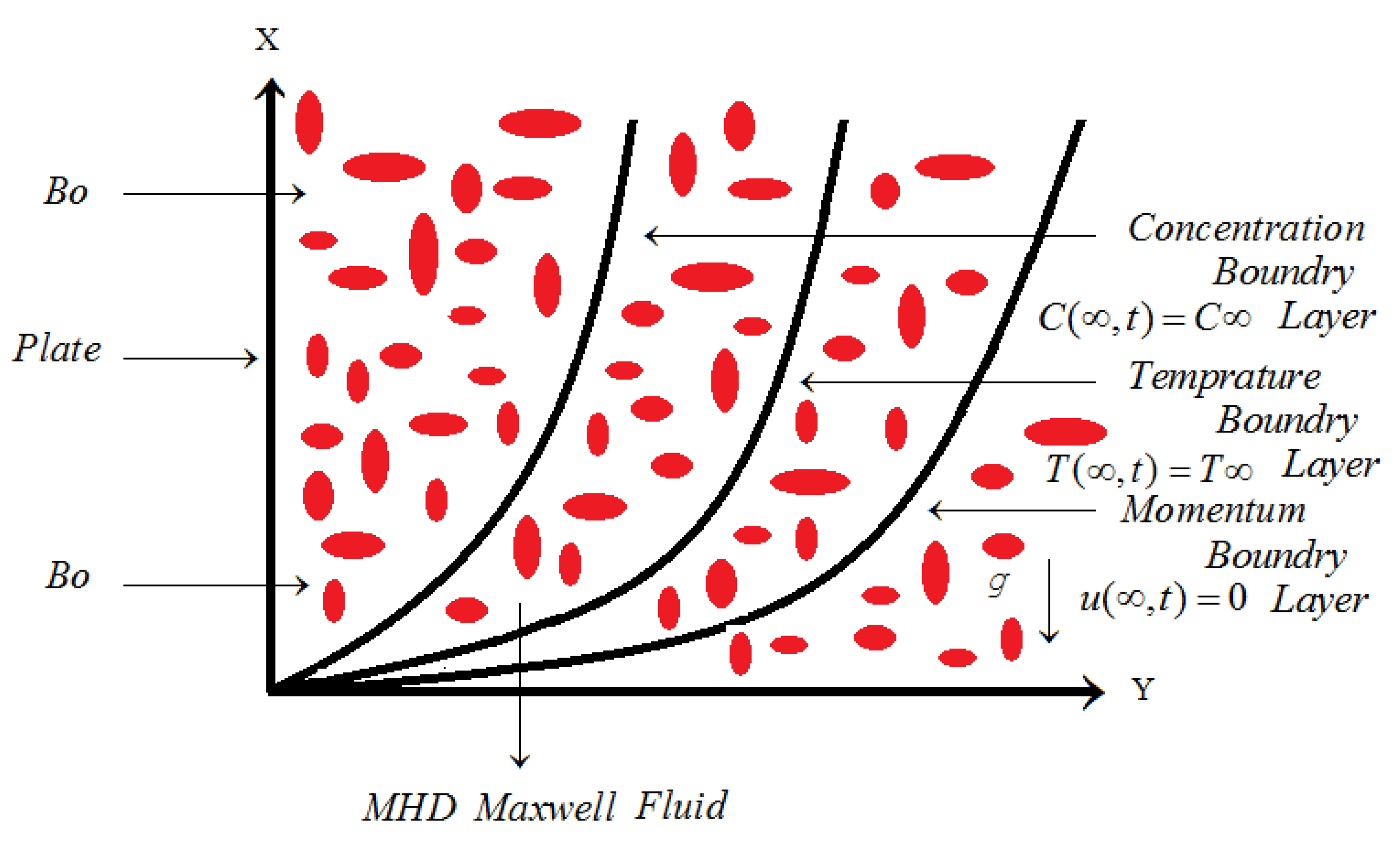
2. Mathematical Model

Let us assume that the unsteady MHD, natural convection, in-compressible, time dependent, viscous motion of Maxwell fluid is very close to an infinite vertical plate embedded in a permeable medium with constant concentration and ramped conditions on temperature. In this case, consider the cartesian coordinates system (x,y); the plate is placed in a plane such as the vertically oriented x-axis and the y-axis in normal direction. Initially, for $t=0$, the fluid and plate exhibit no motion and both possess uniform temperature $T_{\infty }$ and concentration $C_{\infty }$. Moreover, the velocity can be stated piece-wise such that for $0<t\le t_0$, it depends on time as $u(0,t)=u_0(t/t_0)$, and later for $t>t_0$, the plate describes a constant motion with velocity $u_0$. The physical quantities of the models’ flow are described in Figure 1. To model the flow and energy equations, the following principal assumptions are considered:

• Temperature and velocity functions are only composed of variables y and t because the flow is unidirectional and one dimensional.
• Magnetic and radiation effects are neglected along the flow direction.
• The induced magnetic field exerts an insignificant impact on flow.
• Viscous dissipation influence in the temperature equation is neglected.

The principle governing partial differential equations under usual Boussinesq’s approximation with smaller Reynolds number and above mentioned assumptions are modeled as [43,44]:

$$\begin{array}{cc}\hfill & \left(1+{\lambda }_1\frac{\partial }{\partial t}\right)\frac{\partial u^{*}(y,t)}{\partial t}=\upsilon \frac{{\partial }^2{u}^{*}(y,t)}{\partial y^2}-\left(1+{\lambda }_1\frac{\partial }{\partial t}\right)\frac{\sigma B_0^2{u}^{*}(y,t)}{\rho }\hfill \\ & +\left(1+{\lambda }_1\frac{\partial }{\partial t}\right)g{\beta }_{\stackrel{‘}{T}}\left(\stackrel{‘}{T}(y,t)-{\stackrel{‘}{T}}_{\infty }\right)-\left(1+{\lambda }_1\frac{\partial }{\partial t}\right)g{\beta }_{\stackrel{‘}{C}}\left({\stackrel{‘}{C}}_{\infty }-\stackrel{‘}{C}(y,t)\right),\hfill \end{array}$$

(1)

$$\begin{array}{c}\hfill \frac{\partial \stackrel{‘}{T}(y,t)}{\partial t}=\frac{k}{\rho {\stackrel{‘}{C}}_p}\frac{{\partial }^2\stackrel{‘}{T}(y,t)}{\partial y^2},\end{array}$$

(2)

$$\begin{array}{c}\hfill \left(1+{\lambda }_1\frac{\partial }{\partial t}\right)S_0=\upsilon \frac{\partial u^{*}(y,t)}{\partial y},\end{array}$$

(3)

$$\begin{array}{c}\hfill \frac{\partial \stackrel{‘}{C}(y,t)}{\partial t}={\delta }_m\frac{{\partial }^2\stackrel{‘}{C}(y,t)}{\partial y^2}-{\delta }_m\left(\stackrel{‘}{C}(y,t)-{\stackrel{‘}{C}}_{\infty }\right)\end{array}$$

(4)

with initial and boundary conditions

$$\begin{array}{cc}\hfill u^{*}(y,0)& =0,\stackrel{‘}{T}(y,0)={\stackrel{‘}{T}}_{\infty },\stackrel{‘}{C}(y,0)={\stackrel{‘}{C}}_{\infty },\frac{\partial u(y,0)}{\partial t}=0,y\ge 0,\hfill \end{array}$$

(5)

$$\begin{array}{cc}\hfill \stackrel{‘}{C}(0,t)& ={\stackrel{‘}{C}}_w,u^{*}(0,t)=g_1\left(t\right),\stackrel{‘}{T}(0,t)=g_2\left(t\right).\hfill \end{array}$$

(6)

where

$$\begin{array}{c}\hfill g_1\left(t\right)=\left\{\begin{array}{cc}{u}_0\frac{\stackrel{‘}{t}}{t_0},\hfill & 0<\stackrel{‘}{t}\le t_0;\hfill \\ u_0,\hfill & \stackrel{‘}{t}>t_0\hfill \end{array}\right.g_2\left(t\right)=\left\{\begin{array}{cc}(T_w-T_{\infty })\frac{t}{t_0}+T_{\infty },\hfill & 0<t\le t_0;\hfill \\ \stackrel{‘}{T}(0,\stackrel{‘}{t})=T_w,\hfill & t>t_0\hfill \end{array}\right..\end{array}$$

(7)

and

$$\begin{array}{c}\hfill u^{*}(y,t)\to 0,\stackrel{‘}{T}(y,t)\to \infty ,\stackrel{‘}{C}(y,t)\to \infty asy\to \infty .\end{array}$$

(8)

Introducing the set of dimensionless quantities are:

$$\begin{array}{cc}\hfill \psi & =\frac{u_0}{\upsilon }y,\lambda =\frac{{\lambda }_1{u_0}^2}{\upsilon },\tau =\frac{u_0^2}{\upsilon }t,\theta =\frac{\stackrel{‘}{T}-T_{\infty }}{T_w-T_{\infty }},S=\frac{S_0}{\rho u_0},Sc=\frac{\upsilon }{{\delta }_m},G_m=\frac{g{\beta }_{\stackrel{‘}{C}}{t}_0(\stackrel{‘}{C}-C_{\infty })}{u_0},\hfill \\ \hfill u& =\frac{u^{*}}{u_0},M=\frac{{\sigma }_0{B}_0^2\upsilon }{\rho u_0^2},Pr=\frac{\mu C_p}{k},\upsilon =t_0{u_0}^2,C^{*}=\frac{\stackrel{‘}{C}-C_{\infty }}{C_w-C_{\infty }},G_r=\frac{g{\beta }_{\stackrel{‘}{T}}{t}_0(\stackrel{‘}{T}-T_{\infty })}{u_0},{\lambda }_0=\frac{{\upsilon }^2}{u_0^2}.\hfill \end{array}$$

After employing the dimensionless quantities, ignore the asterisk * notation; the following partial differential equations in dimensionless form are derived as:

$$\begin{array}{cc}\hfill \left(1+\lambda \frac{\partial }{\partial \tau }\right)\frac{\partial u(\psi ,\tau )}{\partial \tau }& =\frac{{\partial }^{2}u(\psi ,\tau )}{\partial {\psi }^2}-\left(1+\lambda \frac{\partial }{\partial \tau }\right)Mu(\psi ,\tau )\hfill \\ \hfill & +\left(1+\lambda \frac{\partial }{\partial \tau }\right)G_r\theta (\psi ,\tau )+\left(1+\lambda \frac{\partial }{\partial \tau }\right)G_{m}C(\psi ,\tau ),\hfill \end{array}$$

(9)

$$\begin{array}{c}\hfill \frac{\partial \theta (\psi ,\tau )}{\partial \tau }=\frac{1}{Pr}\frac{{\partial }^2\theta (\psi ,\tau )}{\partial {\psi }^2},\end{array}$$

(10)

$$\begin{array}{c}\hfill \left(1+\lambda \frac{\partial }{\partial \tau }\right)S=\frac{\partial u(\psi ,\tau )}{\partial \psi },\end{array}$$

(11)

$$\begin{array}{c}\hfill \frac{\partial C(\psi ,\tau )}{\partial \tau }=\frac{1}{Sc}\frac{{\partial }^{2}C(\psi ,\tau )}{\partial {\psi }^2}-\frac{{\lambda }_0}{Sc}C(\psi ,\tau ).\end{array}$$

(12)

with conditions in dimensionless form being

$$\begin{array}{c}\hfill u(\psi ,0)=0,C(\psi ,0)=0,\theta (\psi ,0)=0,\end{array}$$

(13)

$$\begin{array}{c}\hfill u(0,\tau )=d\left(\tau \right),\theta (0,\tau )=d\left(\tau \right),C(0,\tau )=1.\end{array}$$

(14)

where

$$\begin{array}{c}\hfill d\left(\tau \right)=\left\{\begin{array}{cc}\tau ,\hfill & 0<\tau \le 1\hfill \\ 1,\hfill & \tau >1\hfill \end{array}\right.,\end{array}$$

$$\begin{array}{c}\hfill u(\psi ,\tau )\to 0,\hspace{1em}C(\psi ,\tau )\to 0,\hspace{1em}\theta (\psi ,\tau )\to 0\hspace{1em}as\hspace{1em}\psi \to \infty .\end{array}$$

(15)

3. Preliminaries

Caputo fractional operator is described as

$$\begin{array}{c}\hfill {}^C{D}_{\eta }^{\wp }f\left(\psi ,\eta \right)=\frac{1}{\Gamma (m-\wp )}{\int }_0^{\eta }\frac{f^n\left(\tau \right)}{{(\eta -\tau )}^{\wp -m+1}}d\tau ,0<\wp <1.\end{array}$$

(16)

and Laplace transformation of Equation (16) is obtained as

$$\begin{array}{c}\hfill \mathcal{L}\left({}^C{D}_{\eta }^{\wp }f\left(z,\eta \right)\right)=s^{\wp }\mathcal{L}\left(f(z,\eta )\right)-s^{\wp -1}f(z,0).\end{array}$$

(17)

where ℘ is named as a fractional parameter.

4. Solution of the Problem

To find the solution to the considered problem, the Laplace transformation technique is employed.

4.1. Exact Solution of Heat Profile with Caputo Time Fractional Derivative

The temperature Equation (10) in terms of Caputo fractional derivative is

$$\begin{array}{c}\hfill {}^C{D}_{\tau }^{\alpha }\theta (\psi ,\tau )=\frac{1}{Pr}\frac{{\partial }^2\theta (\psi ,\tau )}{\partial {\psi }^2},\end{array}$$

(18)

By applying the Laplace Transformation technique to write the solution to Equation (18) with conditions as Equations (13)–(15), we get

$$\begin{array}{c}\hfill \frac{d^2\overline{\theta }(\psi ,s)}{d{\psi }^2}-P_r{s}^{\alpha }\overline{\theta }(\psi ,s)=0.\end{array}$$

(19)

with

$$\begin{array}{c}\hfill \overline{\theta }(0,s)=\frac{1-e^{-s}}{s^2}and\overline{\theta }(\psi ,s)\to 0as\psi \to \infty .\end{array}$$

(20)

Its solution is given by

$$\begin{array}{c}\hfill \overline{\theta }(\psi ,s)=c_1{e}^{\psi \sqrt{P_r{s}^{\alpha }}}+c_2{e}^{-\psi \sqrt{P_r{s}^{\alpha }}}.\end{array}$$

(21)

We applied boundary conditions for temperature given by Equation (20) to determined unknown constants, and we got

$$\begin{array}{c}\hfill \overline{\theta }(\psi ,s)=\left(\frac{1-e^{-s}}{s^2}\right)e^{-\psi \sqrt{P_r{s}^{\alpha }}},\end{array}$$

(22)

which can be written as

$$\begin{array}{cc}\hfill \overline{\theta }(\psi ,s)& =\left(\frac{e^{-\psi \sqrt{P_r{s}^{\alpha }}}}{s^2}\right)-e^{-s}\left(\frac{e^{-\psi \sqrt{P_r{s}^{\alpha }}}}{s^2}\right),\hfill \\ \hfill & ={\overline{\theta }}_c(\psi ,s)-e^{-s}{\overline{\theta }}_c(\psi ,s).\hfill \end{array}$$

(23)

To get the required solution to Equation (23) we used Laplace inverse transformation, which is written as:

$$\begin{array}{c}\hfill \theta (\psi ,\tau )={\theta }_c(\psi ,\tau )-{\theta }_c(\psi ,\Phi )O(\Phi ).\end{array}$$

(24)

where $O(\Phi )$ denotes a standard Heaviside function, $\Phi =\tau -1$ and

$$\begin{array}{c}\hfill {\overline{\theta }}_c(\psi ,s)=\left(\frac{e^{-\psi \sqrt{P_r{s}^{\alpha }}}}{s^2}\right).\end{array}$$

(25)

It is difficult to find ${\theta }_c(\psi ,\tau )$ in exponential form, so we express ${\overline{\theta }}_c(\psi ,s)$ in its equivalent form as

$$\begin{array}{c}\hfill {\overline{\theta }}_c(\psi ,s)=\frac{1}{s^2}+\sum _{n=1}^{\infty }\frac{{(-\psi )}^n{\left(Pr\right)}^{\frac{n}{2}}}{n!}.\frac{1}{s^{2-\frac{n\alpha }{2}}}.\end{array}$$

(26)

Employing inverse Laplace transformation, we get

$$\begin{array}{c}\hfill {\theta }_c(\psi ,\tau )=\tau +\sum _{n=1}^{\infty }\frac{{(-\psi )}^n{\left(Pr\right)}^{\frac{n}{2}}}{n!}.\frac{{\tau }^{1-\frac{n\alpha }{2}}}{\Gamma (2-\frac{n\alpha }{2})}.\end{array}$$

(27)

4.2. Exact Solution of Mass Profile with Caputo Time Fractional Derivative

The fractional version of concentration Equation (12) in the form of Caputo fractional operator is derived as

$$\begin{array}{c}\hfill {}^C{D}_{\tau }^{\alpha }C(\psi ,\tau )=\frac{1}{Sc}\frac{{\partial }^{2}C(\psi ,\tau )}{\partial {\psi }^2}-\frac{{\lambda }_0}{Sc}C(\psi ,\tau ).\end{array}$$

(28)

Solving Equation (28) using (13)–(15) and employing the Laplace Transformation technique, the resulting equations are written as:

$$\begin{array}{c}\hfill \frac{d^2\overline{C}(\psi ,s)}{d{\psi }^2}-\left(S_c{s}^{\alpha }+{\lambda }_0\right)\overline{C}(\psi ,s)=0\end{array}$$

(29)

with

$$\begin{array}{c}\hfill \overline{C}(0,s)=\frac{1}{s}and\overline{C}(\psi ,s)\to 0as\psi \to \infty .\end{array}$$

(30)

The solution in general form is

$$\begin{array}{c}\hfill \overline{C}(\psi ,s)=c_1{e}^{\psi \sqrt{S_c{s}^{\alpha }+{\lambda }_0}}+c_2{e}^{-\psi \sqrt{S_c{s}^{\alpha }+{\lambda }_0}}.\end{array}$$

(31)

The values of constants $c_1$ and $c_2$, conditions are implemented given above Equation (30) for concentration, so

$$\begin{array}{c}\hfill \overline{C}(\psi ,s)=\frac{1}{s}{e}^{-\psi \sqrt{S_c{s}^{\alpha }+{\lambda }_0}}.\end{array}$$

(32)

It is complicated to find $C(\psi ,\tau )$ in exponential form, so $\overline{C}(\psi ,s)$ in its equivalent form is written as

$$\begin{array}{c}\hfill \overline{C}(\psi ,s)=\frac{1}{s}+\sum _{k=1}^{\infty }\sum _{l=0}^{\infty }\frac{{(-\psi )}^k{\left({\lambda }_0\right)}^{\frac{k}{2}-l}{\left(S_c\right)}^l\Gamma (\frac{k}{2}+1)}{k!l!\Gamma (\frac{k}{2}-l+1)}.\frac{1}{s^{1-l\alpha }}.\end{array}$$

(33)

By employing inverse Laplace transformation, we obtained

$$\begin{array}{c}\hfill C(\psi ,\tau )=1+\sum _{k=1}^{\infty }\sum _{l=0}^{\infty }\frac{{(-\psi )}^k{\left({\lambda }_0\right)}^{\frac{k}{2}-l}{\left(S_c\right)}^l\Gamma (\frac{k}{2}+1)}{k!l!\Gamma (\frac{k}{2}-l+1)\Gamma (1-l\alpha )}.{\tau }^{-l\alpha }.\end{array}$$

(34)

4.3. Exact Solution of Velocity Profile with Caputo Time Fractional Derivative

The fractional version of velocity Equation (9) in the form of a Caputo fractional operator is constructed as

$$\begin{array}{cc}\hfill \left(1+{\lambda }^C{D}_{\tau }^{\alpha }\right)\frac{\partial u(\psi ,\tau )}{\partial \tau }& =\frac{{\partial }^{2}u(\psi ,\tau )}{\partial {\psi }^2}-\left(1+{\lambda }^C{D}_{\tau }^{\alpha }\right)Mu(\psi ,\tau )\hfill \\ \hfill & +\left(1+{\lambda }^C{D}_{\tau }^{\alpha }\right)G_r\theta (\psi ,\tau )+\left(1+{\lambda }^C{D}_{\tau }^{\alpha }\right)G_{m}C(\psi ,\tau ),\hfill \end{array}$$

(35)

The solution to Equation (35), by employing Laplace transform, gives the equation in the following form

$$\begin{array}{c}\hfill \left(1+\lambda s^{\alpha }\right)s\overline{u}(\psi ,s)=\frac{d^2\overline{u}(\psi ,s)}{d{\psi }^2}+\left(1+\lambda s^{\alpha }\right)G_r\overline{\theta }\left(\psi ,s\right)+\left(1+\lambda s^{\alpha }\right)G_m\overline{C}\left(\psi ,s\right)-\left(1+\lambda s^{\alpha }\right)M\overline{u}(\psi ,s),\end{array}$$

(36)

$$\begin{array}{c}\hfill \frac{d^2\overline{u}(\psi ,s)}{d{\psi }^2}-\left(1+\lambda s^{\alpha }\right)\left(M+s\right)\overline{u}(\psi ,s)=-\left(1+\lambda s^{\alpha }\right)\left(G_r\overline{\theta }+G_m\overline{C}\right).\end{array}$$

(37)

By using Equations (22) and (32) for placing the values $\overline{\theta }\left(\psi ,s\right)$ and $\overline{C}\left(\psi ,s\right)$, then Equation (37) has the general form of the solution, which is represented as:

$$\begin{array}{cc}\hfill \overline{u}\left(\psi ,s\right)& =c_3{e}^{\psi \sqrt{\left(1+\lambda s^{\alpha }\right)\left(M+s\right)}}+c_4{e}^{-\psi \sqrt{\left(1+\lambda s^{\alpha }\right)\left(M+s\right)}}-\left(\frac{G_r\left(1+\lambda s^{\alpha }\right)\left(1-e^{-s}\right)e^{-\psi \sqrt{P_r{s}^{\alpha }}}}{s^2\left(P_r{s}^{\alpha }-\left(1+\lambda s^{\alpha }\right)\left(M+s\right)\right)}\right)\hfill \\ \hfill & -\left(\frac{G_m\left(1+\lambda s^{\alpha }\right)e^{-\psi \sqrt{S_c{s}^{\alpha }+{\lambda }_0}}}{s\left(S_c{s}^{\alpha }+{\lambda }_0-\left(1+\lambda s^{\alpha }\right)\left(M+s\right)\right)}\right).\hfill \end{array}$$

(38)

Applying $\overline{u}(\psi ,s)\to 0$ as $\psi \to \infty$ and $\overline{u}(0,s)=\frac{1-e^{-s}}{s^2}$, to determine the values of unknowns $c_3$ and $c_4$, we get

$$\begin{array}{cc}\hfill \overline{u}\left(\psi ,s\right)& =\left(\frac{1-e^{-s}}{s^2}\right)e^{-\psi \sqrt{\left(1+\lambda s^{\alpha }\right)\left(M+s\right)}}+\left(\frac{1-e^{-s}}{s^2}\right)\left(\frac{G_r\left(1+\lambda s^{\alpha }\right)\left(e^{-\psi \sqrt{\left(1+\lambda s^{\alpha }\right)\left(M+s\right)}}-e^{-\psi \sqrt{P_r{s}^{\alpha }}}\right)}{P_r{s}^{\alpha }-\left(1+\lambda s^{\alpha }\right)\left(M+s\right)}\right)\hfill \\ \hfill & +\left(\frac{G_m\left(1+\lambda s^{\alpha }\right)\left(e^{-\psi \sqrt{\left(1+\lambda s^{\alpha }\right)\left(M+s\right)}}-e^{-\psi \sqrt{S_c{s}^{\alpha }+{\lambda }_0}}\right)}{s\left(S_c{s}^{\alpha }+{\lambda }_0-\left(1+\lambda s^{\alpha }\right)\left(M+s\right)\right)}\right).\hfill \end{array}$$

(39)

This can be written as

$$\begin{array}{c}\hfill \overline{u}\left(\psi ,s\right)=\overline{u_1}\left(\psi ,s\right)+\overline{u_2}\left(\psi ,s\right)+\overline{u_3}\left(\psi ,s\right).\end{array}$$

(40)

Applying inverse Laplace transformation gives

$$\begin{array}{c}\hfill u\left(\psi ,\tau \right)=u_1\left(\psi ,\tau \right)+u_2\left(\psi ,\tau \right)+u_3\left(\psi ,\tau \right).\end{array}$$

(41)

where

$$\begin{array}{cc}\hfill \overline{u_1}\left(\psi ,s\right)& =\left(\frac{1-e^{-s}}{s^2}\right)e^{-\psi \sqrt{\left(1+\lambda s^{\alpha }\right)\left(M+s\right)}},\hfill \\ \hfill & =\left(\frac{e^{-\psi \sqrt{\left(1+\lambda s^{\alpha }\right)\left(M+s\right)}}}{s^2}\right)-e^{-s}\left(\frac{e^{-\psi \sqrt{\left(1+\lambda s^{\alpha }\right)\left(M+s\right)}}}{s^2}\right),\hfill \\ \hfill & =\overline{u_c}\left(\psi ,s\right)-e^{-s}\overline{u_c}\left(\psi ,s\right),\hfill \\ \hfill u_1\left(\psi ,\tau \right)& =u_c\left(\psi ,\tau \right)-u_c\left(\psi ,\tau -1\right)O(\tau -1).\hfill \end{array}$$

(42)

where $O(\tau -1)$ is a standard Heaviside function. To calculate the value of $u_c\left(\psi ,\tau \right)$, we first express $\overline{u_c}\left(\psi ,s\right)$ in summation form, which is equivalent to exponential form. Therefore, it can be written as

$$\begin{array}{c}\hfill \overline{u_c}(\psi ,s)=\frac{1}{s^2}+\sum _{v=1}^{\infty }\sum _{p=0}^{\infty }\sum _{r=0}^{\infty }\frac{{(-\psi )}^v{\left(M\right)}^{\frac{v}{2}-r}{\left(\lambda \right)}^p{(\Gamma (\frac{v}{2}+1))}^2}{v!p!r!\Gamma (\frac{v}{2}-p+1)\Gamma (\frac{v}{2}-r+1)}.\frac{1}{s^{2-\alpha p-r}}.\end{array}$$

(43)

Employing inverse Laplace transformation, we obtained

$$\begin{array}{c}\hfill u_c(\psi ,\tau )=\tau +\sum _{v=1}^{\infty }\sum _{p=0}^{\infty }\sum _{r=0}^{\infty }\frac{{(-\psi )}^v{\left(M\right)}^{\frac{v}{2}-r}{\left(\lambda \right)}^p{(\Gamma (\frac{v}{2}+1))}^2}{v!p!r!\Gamma (\frac{v}{2}-p+1)\Gamma (\frac{v}{2}-r+1)\Gamma (2-\alpha p-r)}.{\tau }^{1-\alpha p-r}.\end{array}$$

(44)

Next, consider $\overline{u_2}(\psi ,s)$ to calculate $u_2(\psi ,\tau )$:

$$\begin{array}{c}\hfill \overline{u_2}\left(\psi ,s\right)=G_r\left(\frac{1-e^{-s}}{s^2}\right)\left(\frac{\left(1+\lambda s^{\alpha }\right)\left(e^{-\psi \sqrt{\left(1+\lambda s^{\alpha }\right)\left(M+s\right)}}-e^{-\psi \sqrt{P_r{s}^{\alpha }}}\right)}{P_r{s}^{\alpha }-\left(1+\lambda s^{\alpha }\right)\left(M+s\right)}\right).\end{array}$$

(45)

This can be written in modified form as

$$\begin{array}{cc}\hfill \overline{u_2}\left(\psi ,s\right)& =Gr\left(\frac{1-e^{-s}}{s^2}\right)\left[\frac{\left(1+\lambda s^{\alpha }\right)}{P_r{s}^{\alpha }-\left(1+\lambda s^{\alpha }\right)\left(M+s\right)}\right]\left(\left(e^{-\psi \sqrt{\left(1+\lambda s^{\alpha }\right)\left(M+s\right)}}-e^{-\psi \sqrt{P_r{s}^{\alpha }}}\right)\right),\hfill \\ \hfill & =Gr\left[\overline{u_1}(\psi ,s)\overline{u_4}(\psi ,s)-\overline{\theta }(\psi ,s)\overline{u_4}(\psi ,s)\right].\hfill \end{array}$$

(46)

Taking inverse Laplace transformation yields

$$\begin{array}{c}\hfill u_2\left(\psi ,\tau \right)=Gr\left[\left(u_1*u_4\right)\left(\tau \right)-\left(\theta *u_4\right)\left(\tau \right)\right].\end{array}$$

(47)

where

$$\begin{array}{c}\hfill \overline{u_4}(\psi ,s)=\sum _{\eta =0}^{\infty }\sum _{\xi =0}^{\infty }\frac{{(-1)}^{\xi +1}{\left(Pr\right)}^{\eta }{\left(M\right)}^{\xi }\Gamma (\eta +\xi +1)}{{\left(\lambda \right)}^{\eta }\eta !\xi !}.\frac{s^{\alpha \eta -\eta -\xi -1}}{{(s^{\alpha }+\frac{1}{\lambda })}^{\eta }}.\end{array}$$

(48)

Employing inverse Laplace transformation, we obtained

$$\begin{array}{c}\hfill u_4(\psi ,\tau )=\sum _{\eta =0}^{\infty }\sum _{\xi =0}^{\infty }\frac{{(-1)}^{\xi +1}{\left(Pr\right)}^{\eta }{\left(M\right)}^{\xi }\Gamma (\eta +\xi +1)}{{\left(\lambda \right)}^{\eta }\eta !\xi !}.G_{\alpha ,\alpha \eta -\eta -\xi -1,\eta }(\frac{-1}{\lambda },\tau ).\end{array}$$

(49)

similarly, the solution for $u_3\left(\psi ,\tau \right)$ by considering $\overline{u_3}\left(\psi ,s\right)$ is derived, so we write

$$\begin{array}{cc}\hfill \overline{u_3}\left(\psi ,s\right)& =\left(\frac{G_m\left(1+\lambda s^{\alpha }\right)\left(e^{-\psi \sqrt{\left(1+\lambda s^{\alpha }\right)\left(M+s\right)}}-e^{-\psi \sqrt{S_c{s}^{\alpha }+{\lambda }_0}}\right)}{s\left(S_c{s}^{\alpha }+{\lambda }_0-\left(1+\lambda s^{\alpha }\right)\left(M+s\right)\right)}\right),\hfill \\ \hfill & =\frac{G_m}{s}\left[\frac{\left(1+\lambda s^{\alpha }\right)}{\left(S_c{s}^{\alpha }+{\lambda }_0-\left(1+\lambda s^{\alpha }\right)\left(M+s\right)\right)}\right]\left(e^{-\psi \sqrt{\left(1+\lambda s^{\alpha }\right)\left(M+s\right)}}-e^{-\psi \sqrt{S_c{s}^{\alpha }+{\lambda }_0}}\right),\hfill \\ \hfill & =Gm\left[\overline{u_5}(\psi ,s)\overline{u_6}(\psi ,s)-\overline{C}(\psi ,s)\overline{u_6}(\psi ,s)\right].\hfill \end{array}$$

(50)

Finally, by applying Laplace inverse transformation, we get

$$\begin{array}{c}\hfill u_3\left(\psi ,\tau \right)=Gm\left[\left(u_5*u_6\right)\left(\tau \right)-\left(C*u_6\right)\left(\tau \right)\right].\end{array}$$

(51)

where

$$\begin{array}{cc}\hfill \overline{u_5}\left(\psi ,s\right)& =\left(\frac{e^{-\psi \sqrt{\left(1+\lambda s^{\alpha }\right)\left(M+s\right)}}}{s}\right),\hfill \\ \hfill \overline{u_5}(\psi ,s)& =\frac{1}{s}+\sum _{v=1}^{\infty }\sum _{p=0}^{\infty }\sum _{r=0}^{\infty }\frac{{(-\psi )}^v{\left(M\right)}^{\frac{v}{2}-r}{\left(\lambda \right)}^p{(\Gamma (\frac{v}{2}+1))}^2}{v!p!r!\Gamma (\frac{v}{2}-p+1)\Gamma (\frac{v}{2}-r+1)}.\frac{1}{s^{1-\alpha p-r}}.\hfill \end{array}$$

(52)

Employing inverse Laplace transformation, we obtained

$$\begin{array}{c}\hfill u_5(\psi ,\tau )=1+\sum _{v=1}^{\infty }\sum _{p=0}^{\infty }\sum _{r=0}^{\infty }\frac{{(-\psi )}^v{\left(M\right)}^{\frac{v}{2}-r}{\left(\lambda \right)}^p{(\Gamma (\frac{v}{2}+1))}^2}{v!p!r!\Gamma (\frac{v}{2}-p+1)\Gamma (\frac{v}{2}-r+1)\Gamma (1-\alpha p-r)}.{\tau }^{-\alpha p-r}.\end{array}$$

(53)

Furthermore,

$$\begin{array}{c}\hfill \overline{u_6}(\psi ,s)=\sum _{\eta =0}^{\infty }\sum _{\xi =0}^{\infty }\sum _{ϵ=0}^{\infty }\frac{{(-1)}^{\xi +1}{\left(Sc\right)}^{ϵ}{\left(M\right)}^{\xi }{\left({\lambda }_0\right)}^{\eta -ϵ}\Gamma (\eta +\xi +1)}{{\left(\lambda \right)}^{\eta }ϵ!\xi !\Gamma (\eta -ϵ+1)}.\frac{s^{\alpha ϵ-\eta -\xi -1}}{{(s^{\alpha }+\frac{1}{\lambda })}^{\eta }}.\end{array}$$

(54)

Employing inverse Laplace transformation, we obtained

$$\begin{array}{c}\hfill u_6(\psi ,\tau )=\sum _{\eta =0}^{\infty }\sum _{\xi =0}^{\infty }\sum _{ϵ=0}^{\infty }\frac{{(-1)}^{\xi +1}{\left(Sc\right)}^{ϵ}{\left(M\right)}^{\xi }{\left({\lambda }_0\right)}^{\eta -ϵ}\Gamma (\eta +\xi +1)}{{\left(\lambda \right)}^{\eta }ϵ!\xi !\Gamma (\eta -ϵ+1)}.G_{\alpha ,\alpha ϵ-\eta -\xi -1,\eta }(\frac{-1}{\lambda },\tau ).\end{array}$$

(55)

The function $G_{a,b,c}(.,\tau )$ used in the above expressions is known as the Generalized Lorenzo Hartly function, and its Laplace inverse is defined as: ${\mathcal{L}}^{-1}\left\{\frac{s^b}{{(s^a-d)}^c}\right\}=G_{a,b,c}(d,\tau )$; $Re(ac-b)>0$, $Re\left(s\right)>0$, $\left|\frac{d}{s^a}\right|<1$.

4.4. Solution of Shear Stress

The fractional version of Equation (11) in the form of a Caputo fractional operator is constructed as

$$\begin{array}{c}\hfill \left(1+{\lambda }^C{D}_{\tau }^{\alpha }\right)S=\frac{\partial u(\psi ,\tau )}{\partial \psi }.\end{array}$$

(56)

The solution to Equation (56), obtained by employing Laplace transform, is

$$\begin{array}{c}\hfill \left(1+\lambda s^{\alpha }\right)\overline{S}\left(\psi ,s\right)=\frac{d\overline{u}\left(\psi ,s\right)}{d\psi }.\end{array}$$

(57)

To find the value of $\frac{d\overline{u}\left(\psi ,s\right)}{d\psi }$, differentiating Equation (39) with respect to $\psi$ yields

$$\begin{array}{cc}\hfill \frac{d\overline{u}\left(\psi ,s\right)}{d\psi }& =\left(\frac{1-e^{-s}}{s^2}\right)\left(-\sqrt{\S }{e}^{-\psi \sqrt{\S }}\right)+\left(\frac{1-e^{-s}}{s^2}\right)\left(\frac{G_r\left(1+\lambda s^{\alpha }\right)\left(-\sqrt{\S }{e}^{-\psi \sqrt{\S }}+\sqrt{P_r{s}^{\alpha }}{e}^{-\psi \sqrt{P_r{s}^{\alpha }}}\right)}{P_r{s}^{\alpha }-\S }\right)\hfill \\ \hfill & +\left(\frac{G_m\left(1+\lambda s^{\alpha }\right)\left(-\sqrt{\S }{e}^{-\psi \sqrt{\S }}+\sqrt{S_c{s}^{\alpha }+{\lambda }_0}{e}^{-\psi \sqrt{S_c{s}^{\alpha }+{\lambda }_0}}\right)}{s\left(S_c{s}^{\alpha }+{\lambda }_0-\S \right)}\right).\hfill \end{array}$$

(58)

where $\S =\left(1+\lambda s^{\alpha }\right)\left(M+s\right)$.

Substituting Equation (58) into Equation (57), which gives the solution of shear stress:

$$\begin{array}{cc}\hfill \overline{S}\left(\psi ,s\right)& =\left(\frac{1-e^{-s}}{s^2}\right)\left(\frac{-\sqrt{\S }{e}^{-\psi \sqrt{\S }}}{1+\lambda s^{\alpha }}\right)+\left(\frac{1-e^{-s}}{s^2}\right)\left(\frac{G_r\left(-\sqrt{\S }{e}^{-\psi \sqrt{\S }}+\sqrt{P_r{s}^{\alpha }}{e}^{-\psi \sqrt{P_r{s}^{\alpha }}}\right)}{P_r{s}^{\alpha }-\S }\right)\hfill \\ \hfill & +\left(\frac{G_m\left(-\sqrt{\S }{e}^{-\psi \sqrt{\S }}+\sqrt{S_c{s}^{\alpha }+{\lambda }_0}{e}^{-\psi \sqrt{S_c{s}^{\alpha }+{\lambda }_0}}\right)}{s\left(S_c{s}^{\alpha }+{\lambda }_0-\S \right)}\right).\hfill \end{array}$$

(59)

Since the solutions given in Equation (59) contain complex terms of the Laplace parameter s, to derive the solution in a real time $\tau$, we applied numerical inversion method known as Durbin Method [57].

5. Limiting Cases

As $\alpha \to 1$, we get the same expression for velocity profile as Talha Anwar et al. [56] obtained with ramped temperature, without considering the term $Gm$, i.e, $Gm=0$. Furthermore, we derive the same result for velocity profile and temperature distribution of a viscous fluid when $\lambda =0$ and $Gm=0$ as Seth et al. [58]. This proves the authenticity of our newly established solution expressions.

6. Results and Discussion

In this paper, we investigated the effects of constant concentration, temperature, and velocity with ramped conditions on time-dependent MHD convective flow of Maxwell fluid. We derived exact solution expressions in terms of special functions for dimensionless velocity, concentration, and ramped wall temperature via a Caputo fractional time operator by using the method of Laplace transformation as in the existing literature. To analyze the physical importance of the proposed problem, estimated the results with the help of graphically illustration for several values of various parameters involved in the problem such as Schmidt number $Sc$, Prandtl number $Pr$, magnetic number M, mass Grashof number $Gm$, fractional parameter $\alpha$, and thermal Grashof number $Gr$. In Figure 2, Figure 3, Figure 4, Figure 5, Figure 6, Figure 7 and Figure 8; behavior of temperature, concentration, and velocity are discussed for two different values of $\alpha$. In Figure 9, Figure 10, Figure 11, Figure 12, Figure 13, Figure 14 and Figure 15, we compare the classical result with the Caputo fractional time derivative for temperature, concentration, and velocity for involved parameters in the considered problem, and Figure 16, Figure 17 and Figure 18 present graphs for varying values of $\alpha$.

Figure 2 describes the temperature for distinct values of $Pr$ with $\alpha =0.1$ and $\alpha =0.9$; when the value of $Pr$ increases, the result is falling the temperature. Figure 3 illustrates the behavior of the concentration curve for various values of the Schmidt number $Sc$ parameter with $\alpha =0.1$ and $\alpha =0.9$; it is deceptive that for maximum values of $Sc$, the concentration curve decays. The involvement of the concentration factor of fluid velocity on the fluid flow is very important and cannot be overlooked.

Figure 4 describes the effects of $Gm$ when $\alpha =0.1$ and $\alpha =0.9$. The mass Grashof number is generally defined as the ratio of mass buoyancy force to viscous force, which causes unrestricted convection. It is noticed that the velocity is enhanced in the case of high values of $Gm$. Figure 5 presents the impacts of $Gr$ with $\alpha =0.1$ and $\alpha =0.9$. It is remarked that the velocity contour is elevated due to the large values of $Gr$. Thermal Grashof number is the proportion of thermal buoyancy force to viscous force, which causes free convection. Figure 6 illustrates the variation in velocity field for different values of M with $\alpha =0.1$ and $\alpha =0.9$; it can be observed that the fluid velocity declines when M is maximum, causing an increase in the Lorentz force, which act as a dragging force along with allied forces, thereby leading to a fall in the fluid velocity. Furthermore, this force becomes weaker when this is far away from the plate surface, and eventually fluid flow stops. In Figure 7, the impact of $Pr$ on the velocity with $\alpha =0.1$ and $\alpha =0.9$ is analyzed. It causes a reduced fluid velocity for every increase in the values of $Pr$. In Figure 8, the effect of $Sc$ with $\alpha =0.1$ and $\alpha =0.9$ on velocity profile is analyzed: the flow decreases as Sc increases. Schmidt number $Sc$ signifies concentration, and velocity in free convection flow regimes of fluids are by the relative effectiveness momentum.

In Figure 9, Figure 10, Figure 11, Figure 12, Figure 13, Figure 14 and Figure 15, we observe that temperature, concentration and velocity profile with the Caputo fractional time derivative displays more decay than the classical approach presented by Talha Anwar et al. [56]. Therefore, it is concluded that the Caputo fractional derivative used in the present paper efficiently shows the decay in temperature field, concentration, and velocity profile compared to the classical approach. Furthermore, in Figure 16, Figure 17 and Figure 18, it is noticed that we recovered the classical result as $\alpha \to 1$.

7. Conclusions

In this paper, we analyzed the effects of ramped temperature and velocity with constant concentration on MHD, time-dependent, and convective flows of Maxwell fluids. The governing partial differential equation is inscribed into a dimensionless form. To develop the fractional model by using the modern interpretation of the Caputo fractional time-derivative operator and accomplish the comparison with ordinary models. The Laplace transformation technique is applied to establish the analytical solution for velocity and the concentration and energy equations in terms of special functions for the proposed problem. Furthermore, conferred dissimilar parameters, i.e., Prandtl number $Pr$, Maxwell parameter $\lambda$, fractional parameter $\alpha$, Schmidt number $Sc$, Magnetic field M, and Mass and Thermal Grashof numbers $Gm$ and $Gr$, respectively, were used to analyze the impacts of all these parameters on fluid velocity field, constant concentration, and ramped wall temperature with the help of graphical illustrations. Some noteworthy remarks and concluding results from this work are as follows:

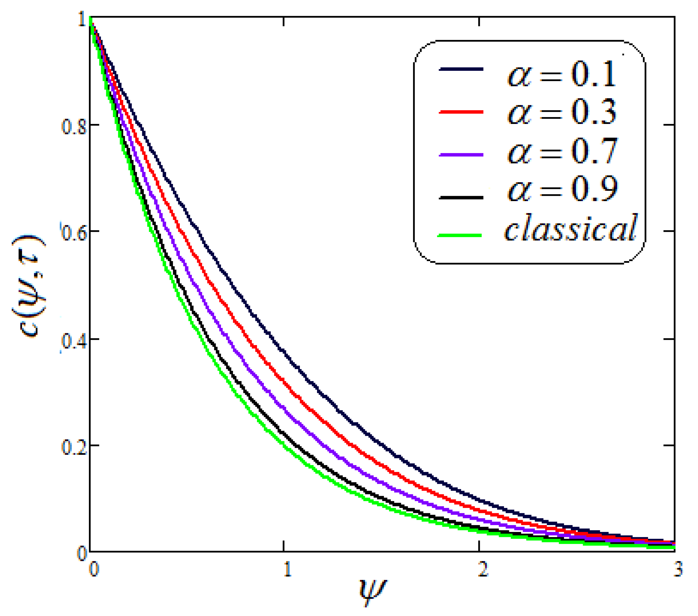
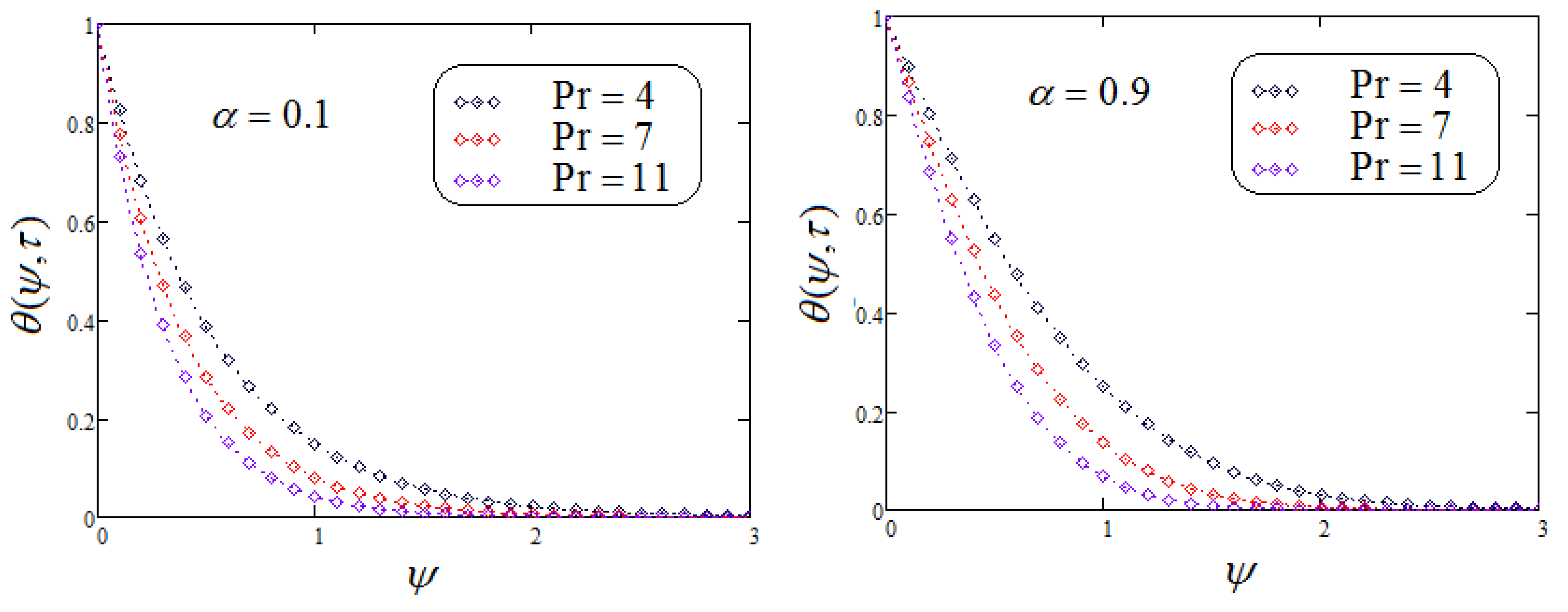
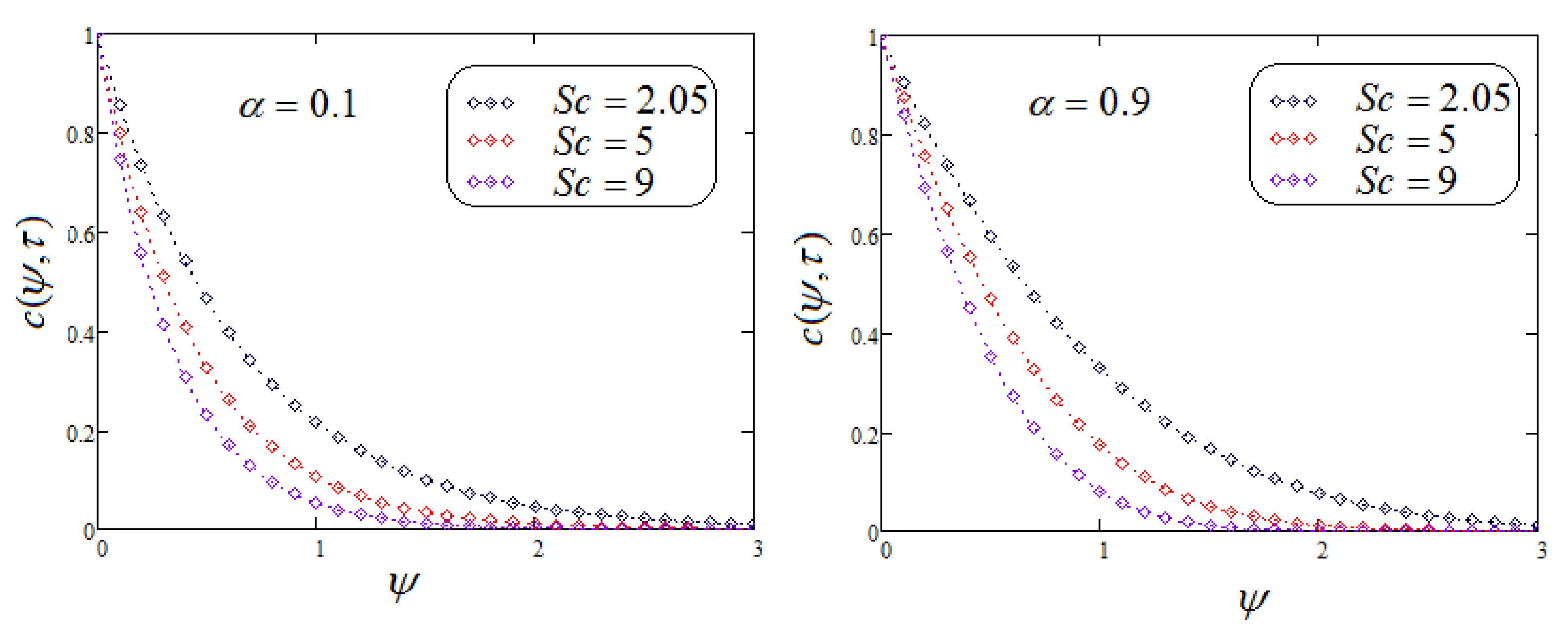
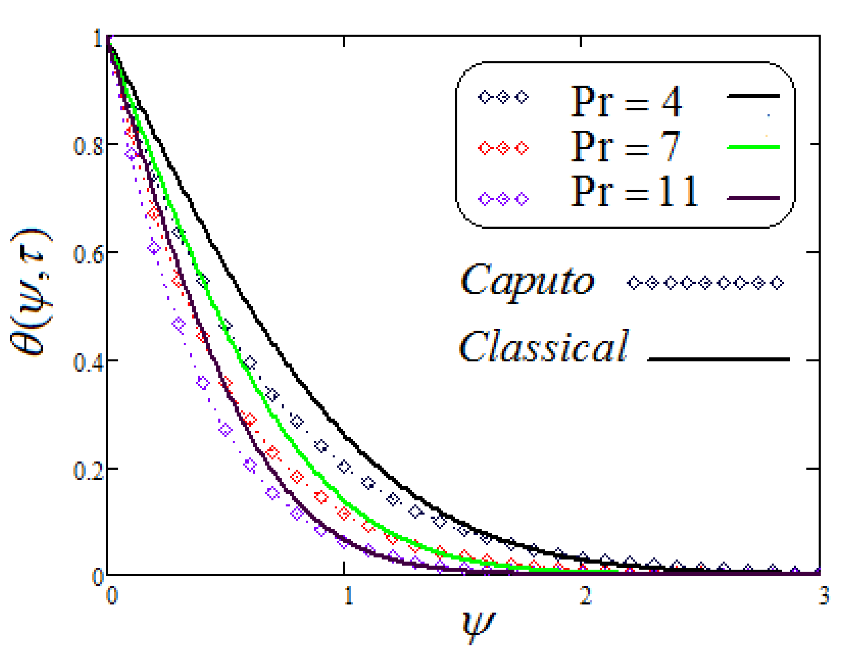
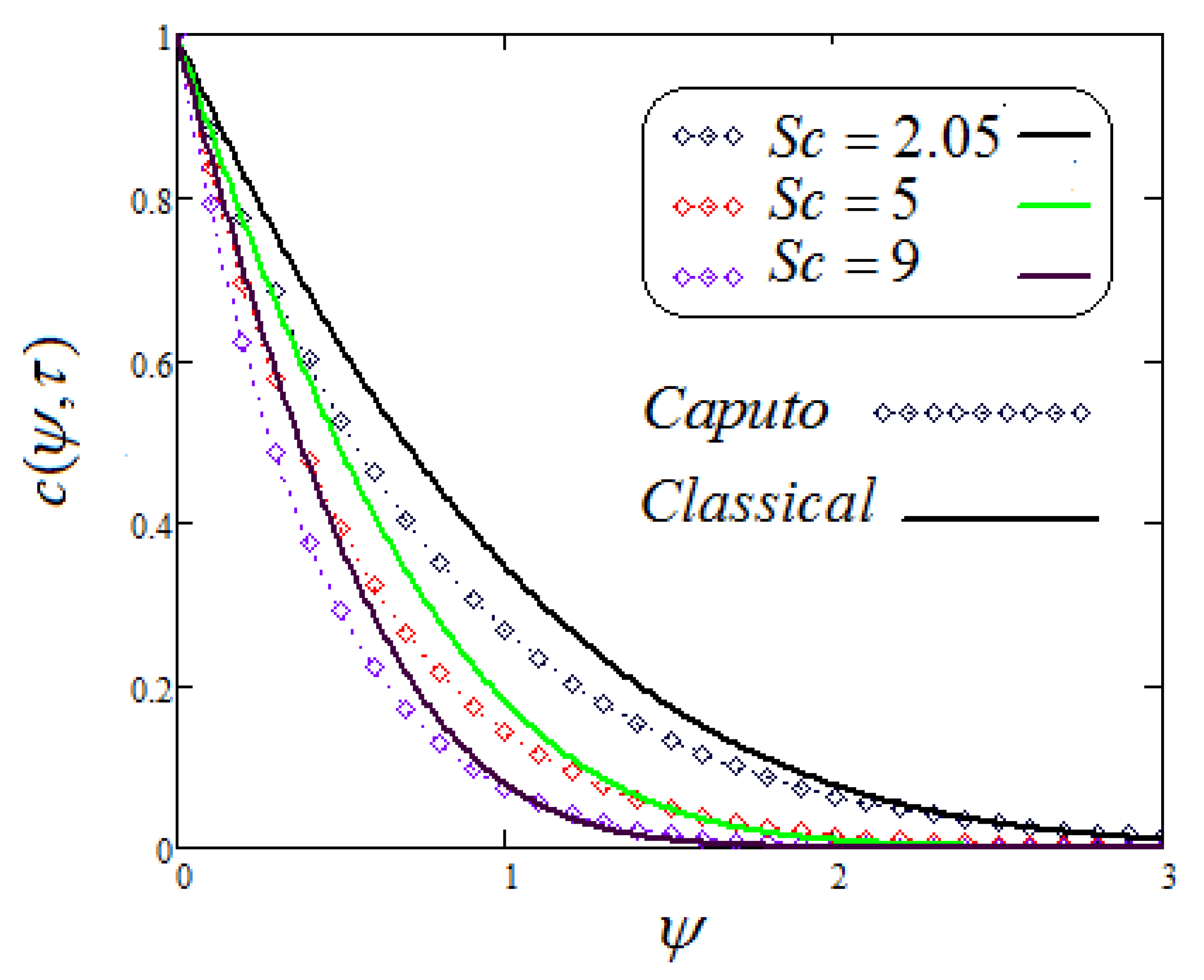
• The temperature field declines with larger values of $P_r$. Furthermore, we noted a reduced concentration for increasing values of $Sc$.
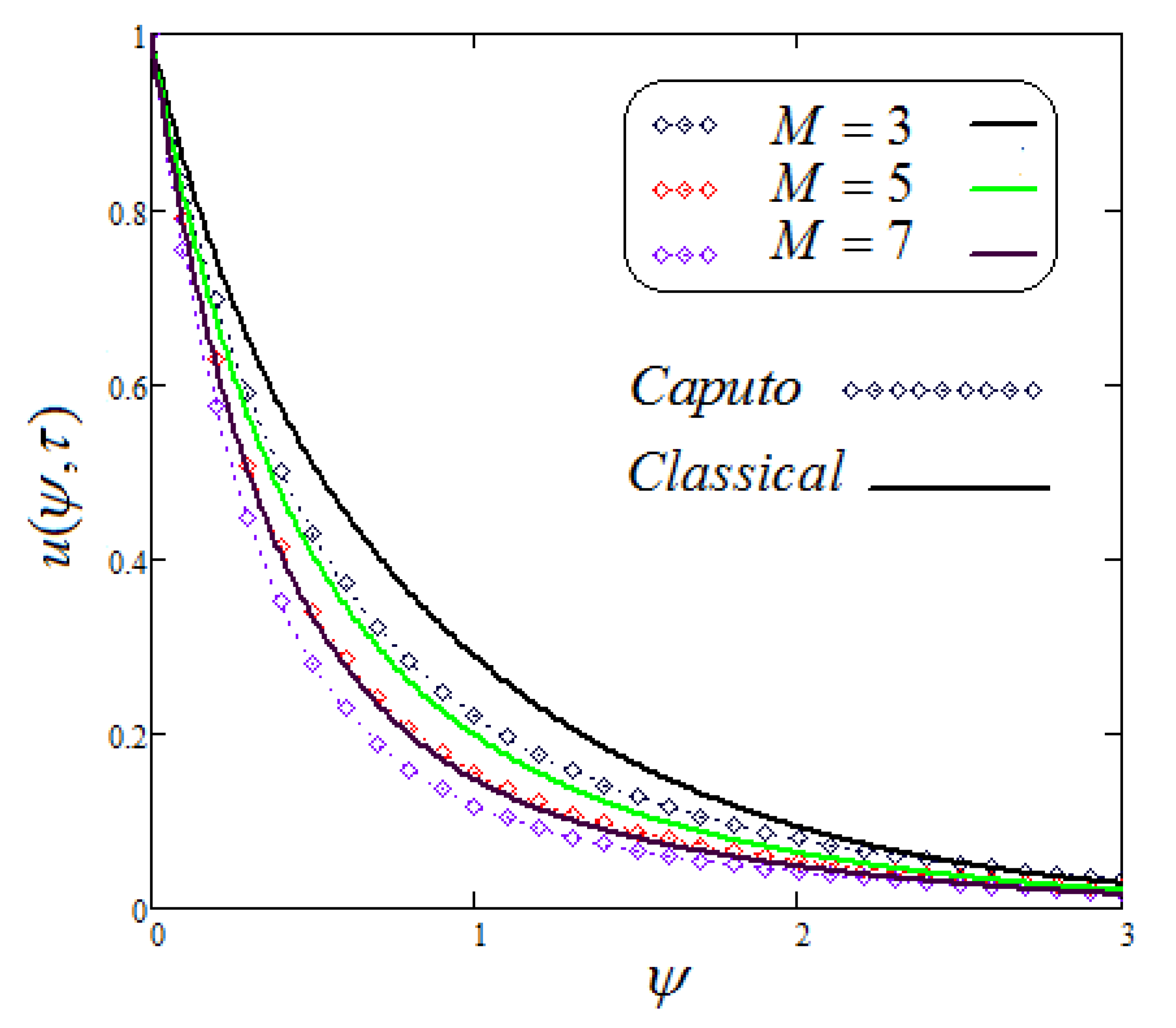
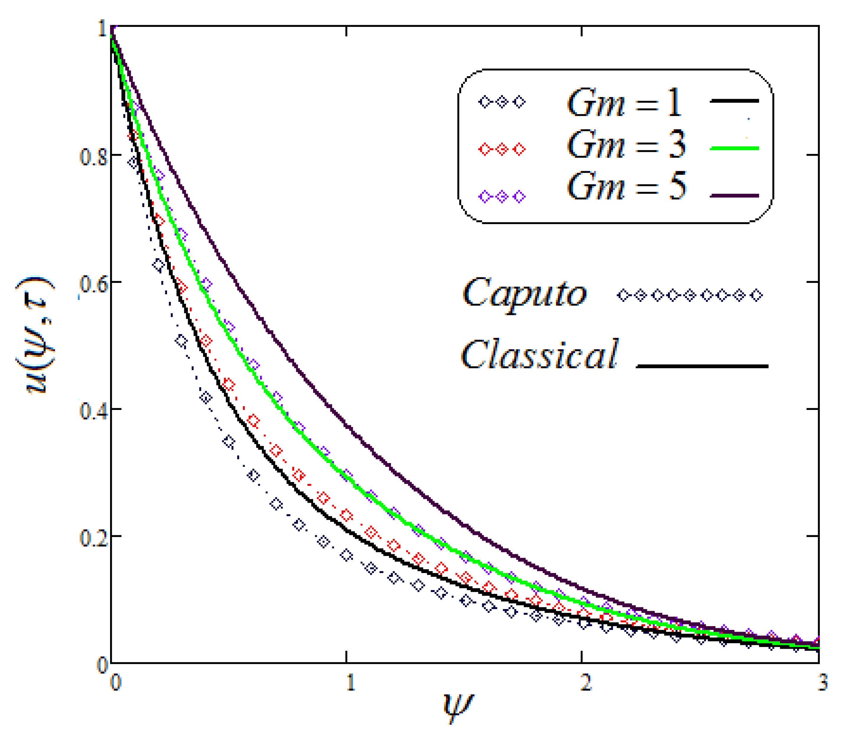
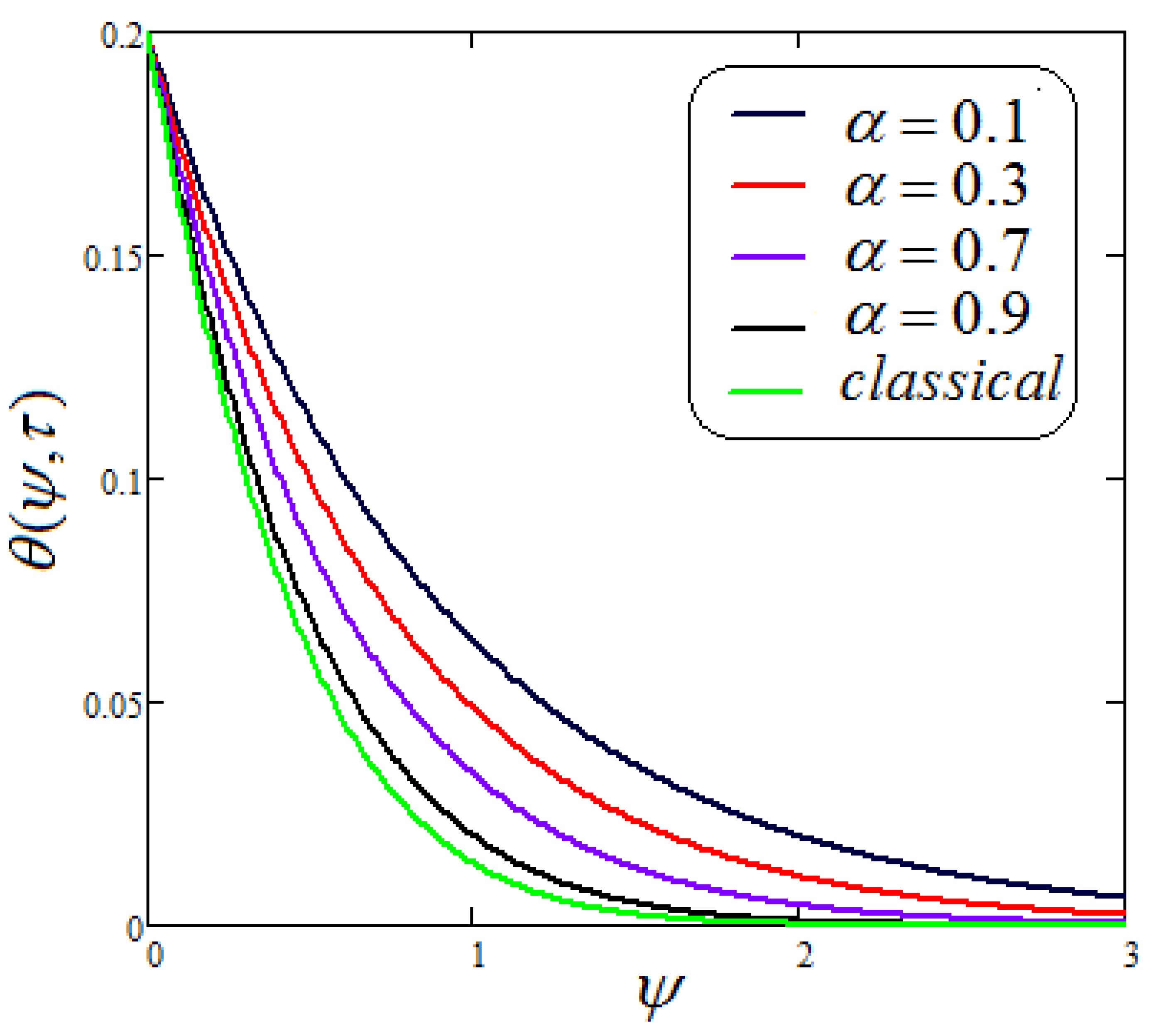
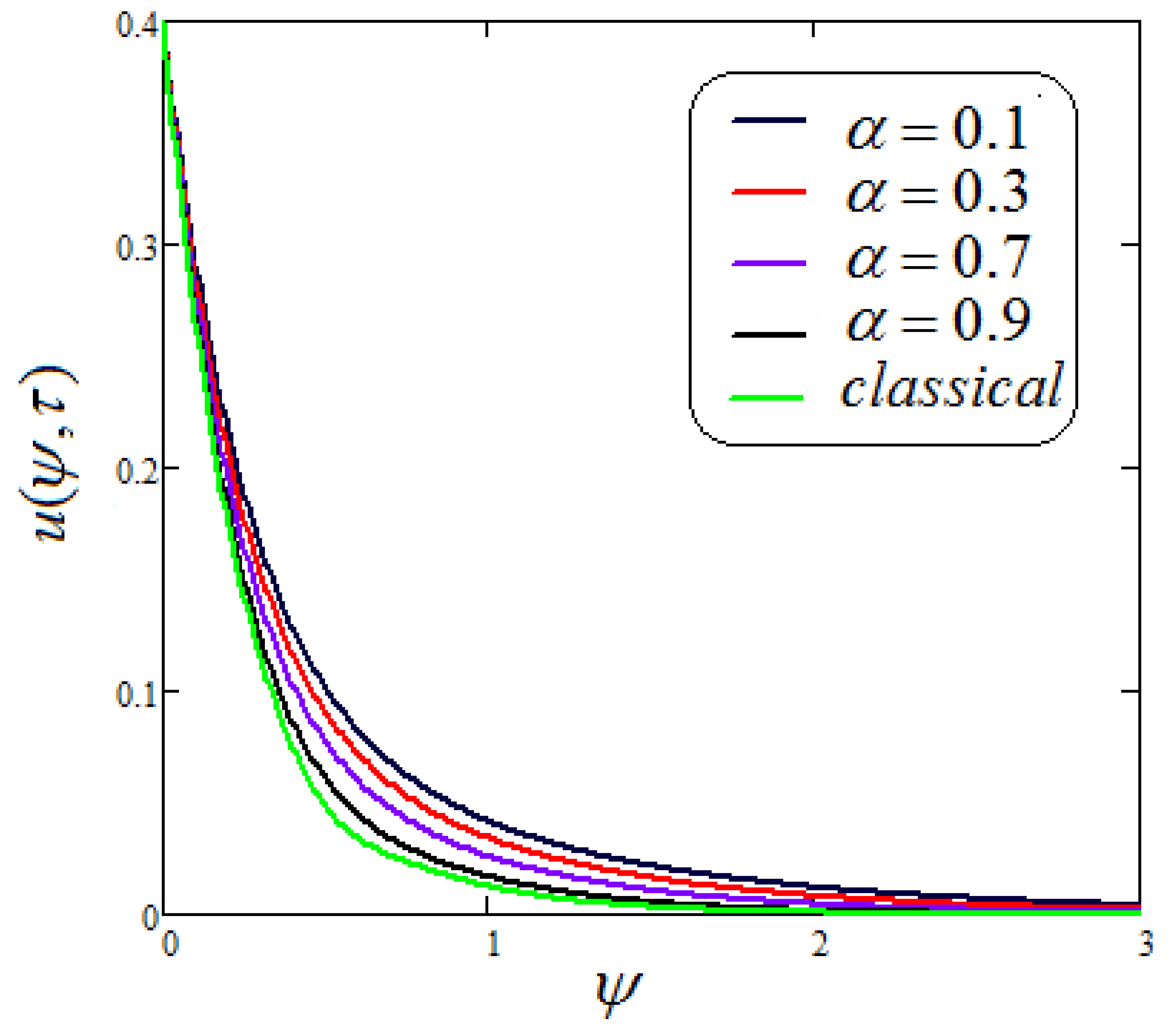
• Curves for Temperature, Concentration, and Velocity are deaccelerated via Caputo as compared to the classical derivative.
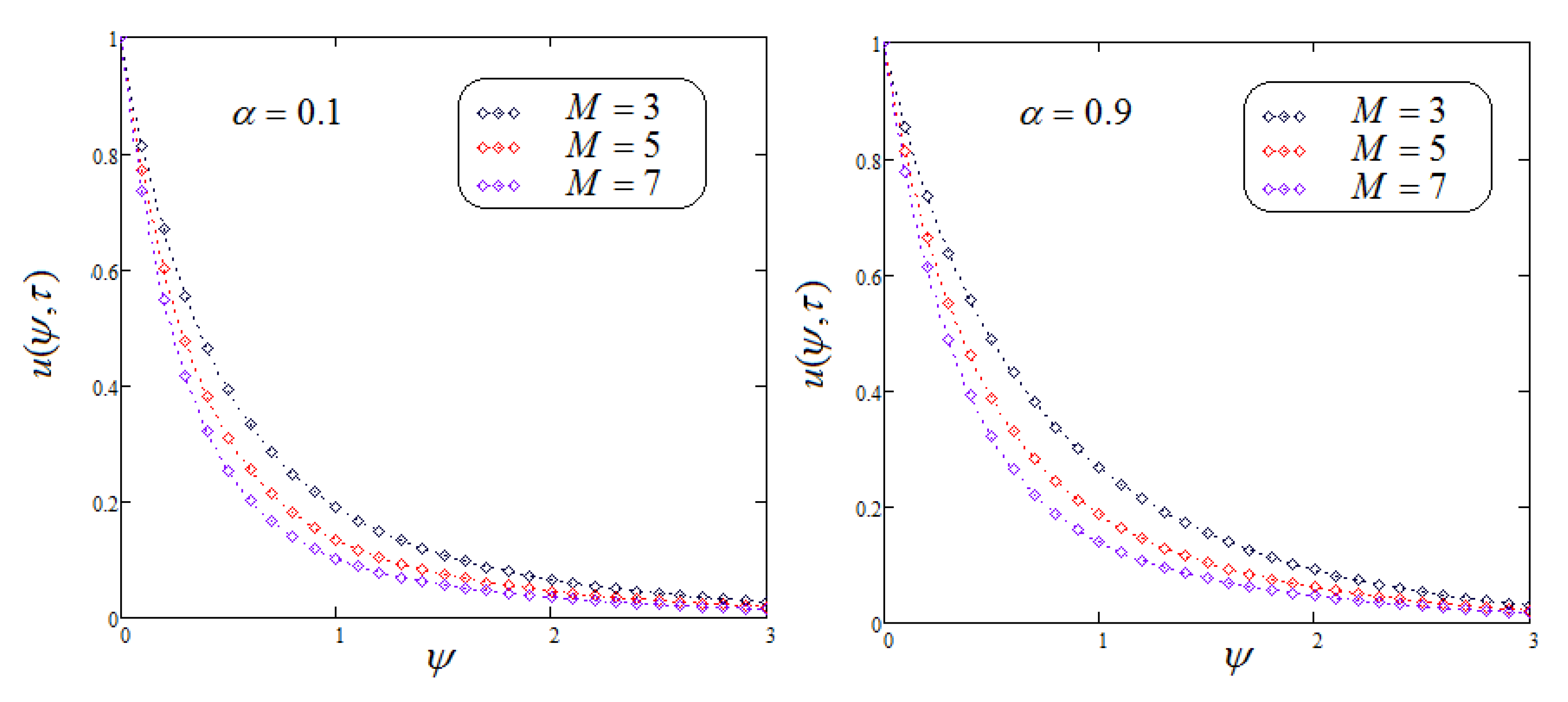
• With higher values of M, the fluid velocity is decreased.
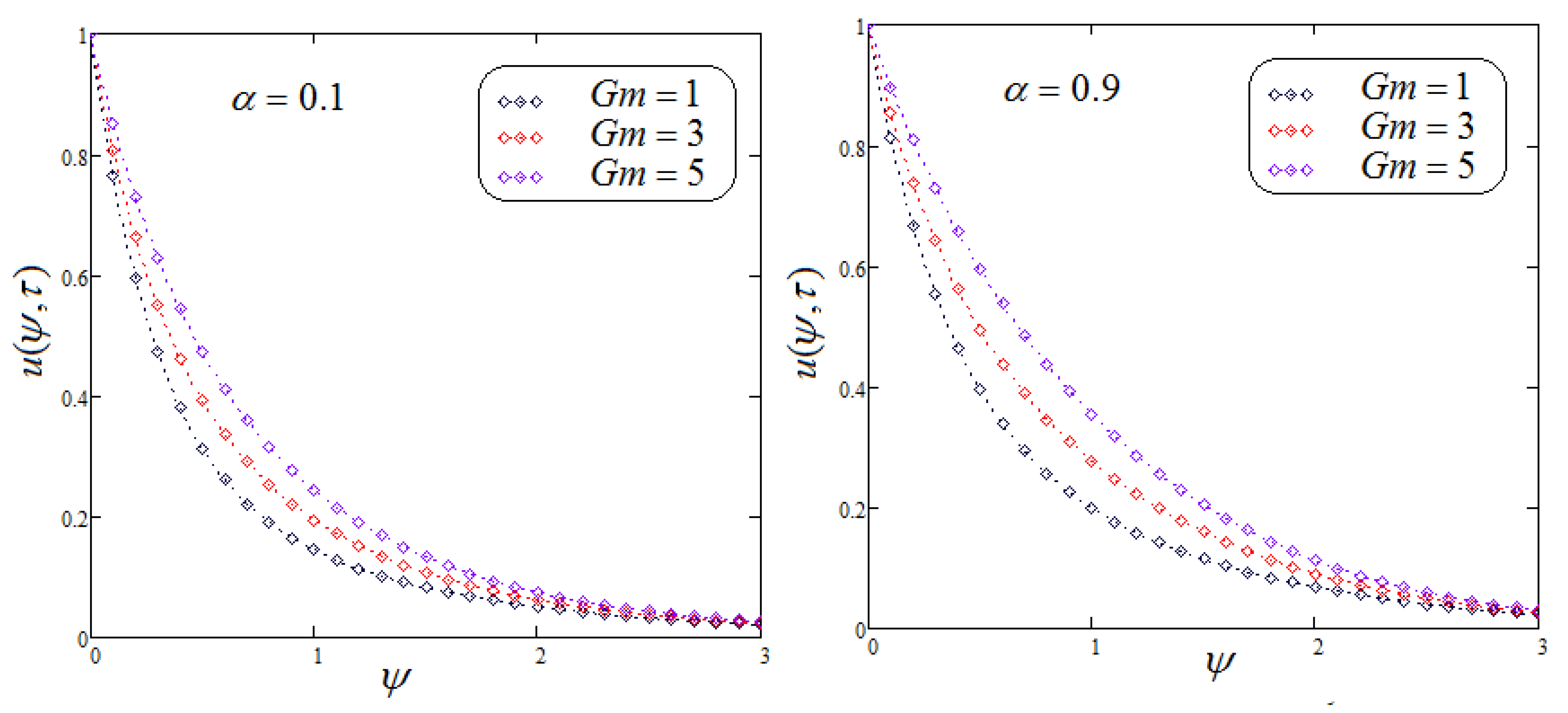
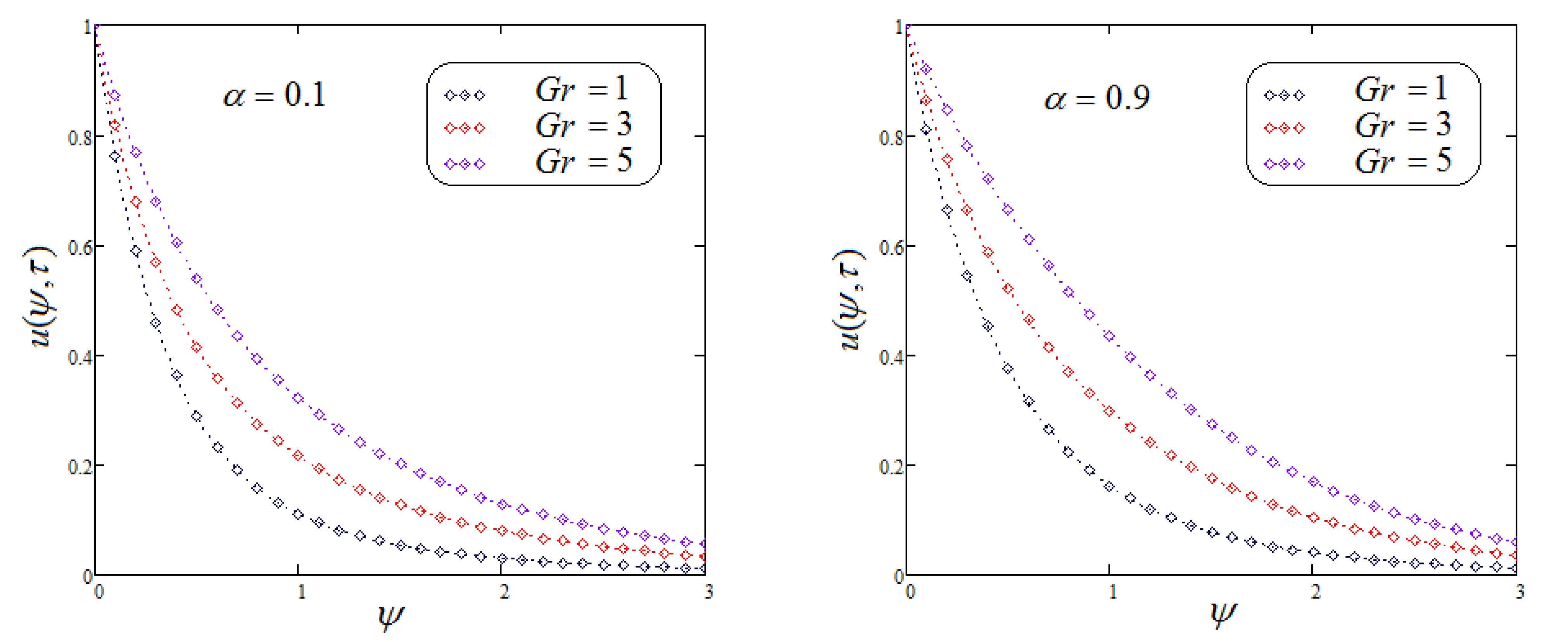
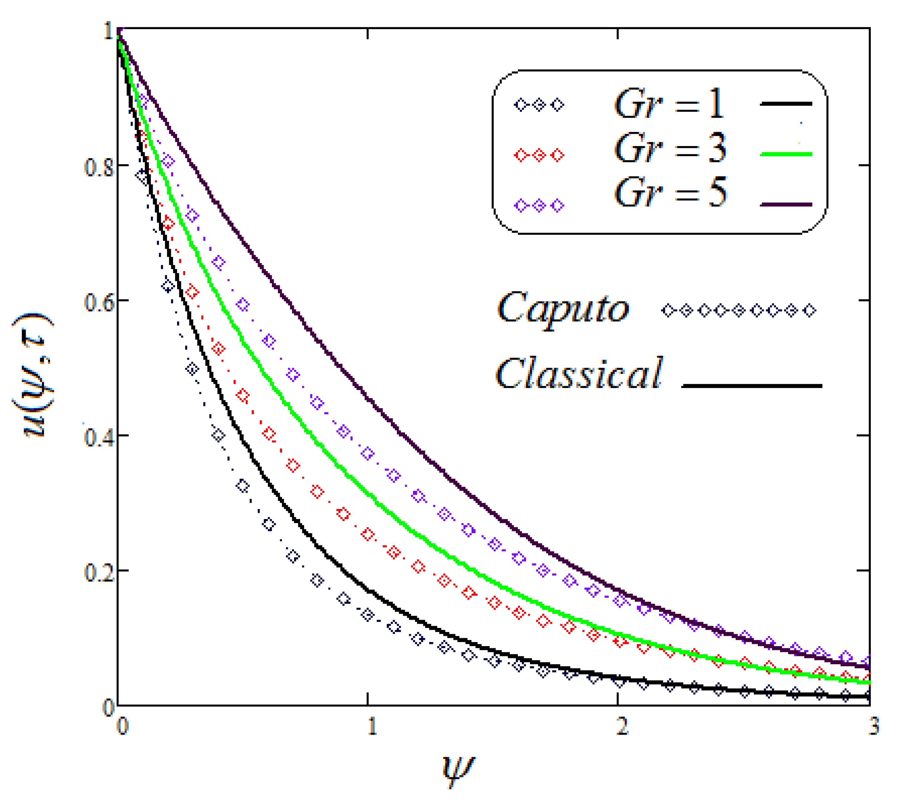
• Increasing values of Grashof numbers $G_r$ and $Gm$ stimulate velocity distribution.
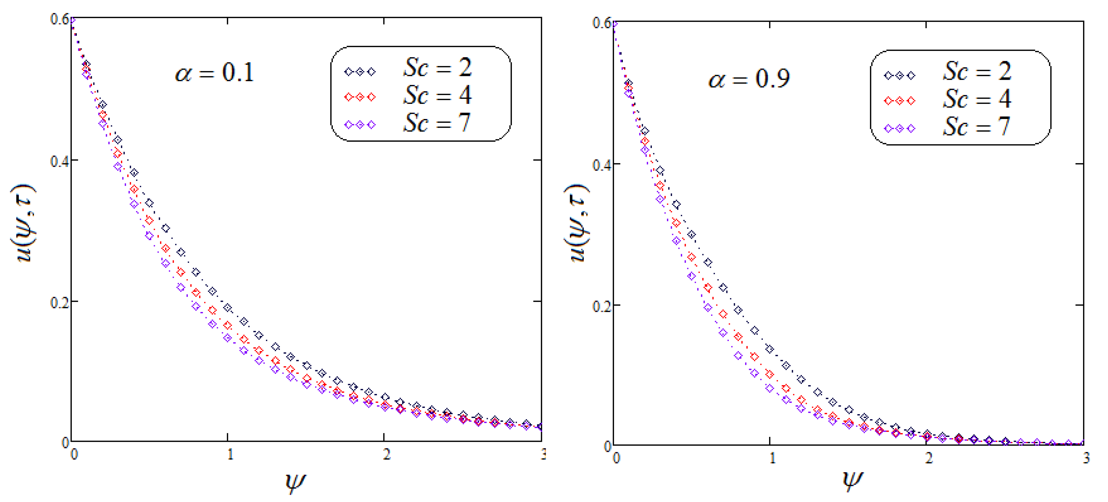
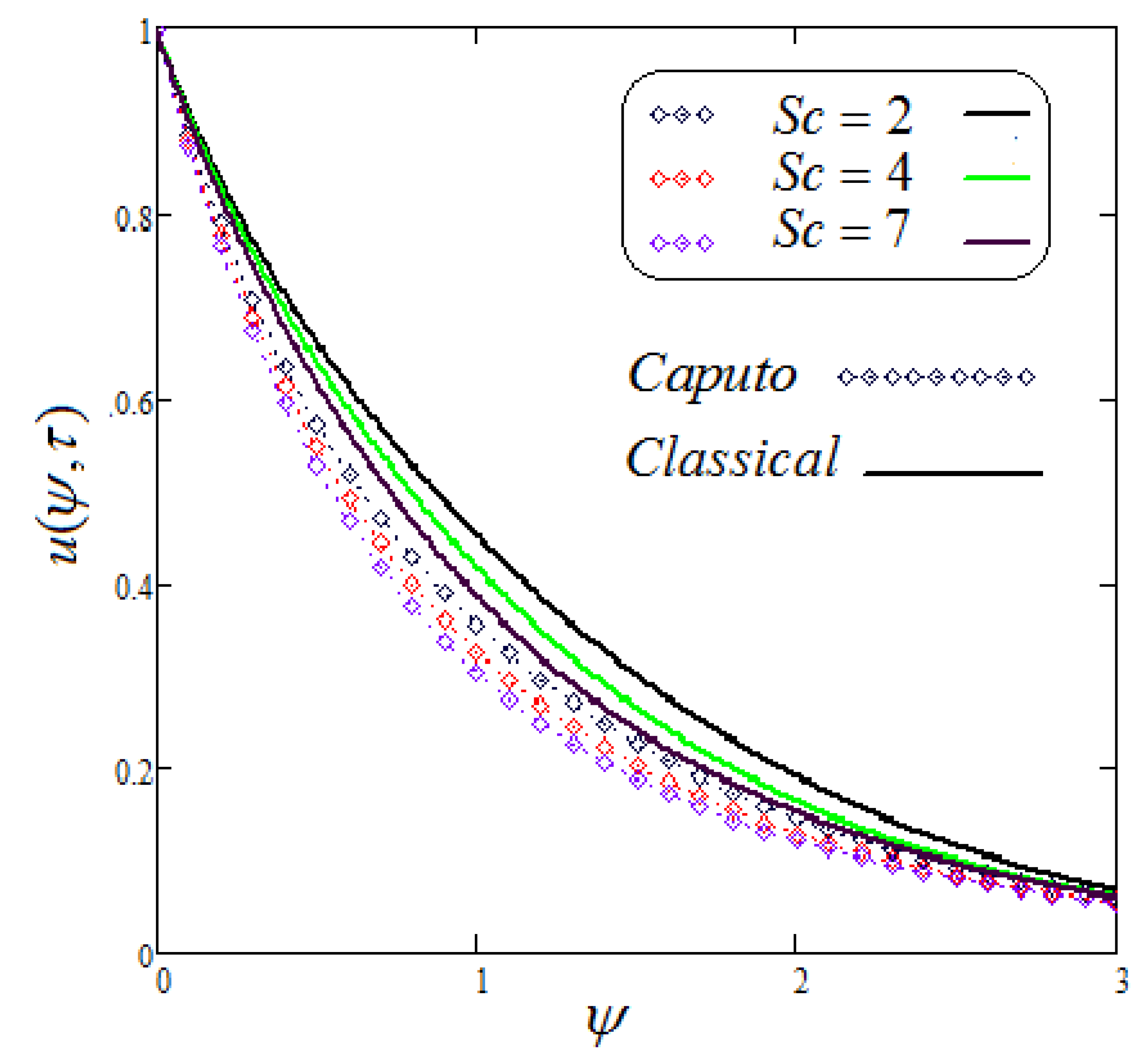
• The accumulative values of the parameters $Sc$ and $P_r$ decrease the velocity distribution.
• The involvement of the concentration factor of fluid velocity in the fluid movement is significant and cannot be overlooked.
• The Caputo fractional time derivative converges to that of the classical model when $\alpha \to 1$.

This work can be extended in future by using the application of various time-fractional operators such as CF, ABC, and CPC.

References

1. Maxwell, J.C.I. IV. On the dynamical theory of gases. Philos. Trans. R. Soc. Lond. 1867, 157, 49–88. [Google Scholar]
2. Jordan, P.; Puri, A.; Boros, G. On a new exact solution to Stokes’ first problem for Maxwell fluids. Int. J. Non-Linear Mech. 2004, 39, 1371–1377. [Google Scholar] [CrossRef]
3. Fetecau, C.; Jamil, M.; Fetecau, C.; Siddique, I. A note on the second problem of Stokes for Maxwell fluids. Int. J. Non-Linear Mech. 2009, 44, 1085–1090. [Google Scholar] [CrossRef]
4. Fetecau, C.; Fetecau, C. A new exact solution for the flow of a Maxwell fluid past an infinite plate. Int. J. Non-Linear Mech. 2003, 38, 423–427. [Google Scholar] [CrossRef]
5. Noor, N.F.M. Analysis for MHD flow of a Maxwell fluid past a vertical stretching sheet in the presence of thermophoresis and chemical reaction. World Acad. Sci. Eng. Technol. 2012, 64, 1019–1023. [Google Scholar]
6. Bhojraj, L.; Abro, K.A.; Abdul, W.S. Thermodynamical analysis of heat transfer of gravity-driven fluid flow via fractional treatment: An analytical study. J. Therm. Anal. Calorim. 2020, 144, 155–165. [Google Scholar] [CrossRef]
7. Solangi, K.H.; Kazi, S.N.; Luhur, M.R.; Badarudin, A.; Amiri, A.; Sadri, R.; Zubir, M.N.M.; Gharehkhani, S.; Teng, K.H. A comprehensive review of thermo-physical properties and convective heat transfer to nanofluids. Energy 2015, 89, 1065e86. [Google Scholar] [CrossRef]
8. Soomro, F.A.; Haq, R.U.; Khan, Z.H.; Zhang, Q. Passive control of nanoparticle due to convective heat transfer of Prandtl fluid model at the stretching surface. Chin. J. Phys. 2017, 55, 1561–1568. [Google Scholar] [CrossRef]
9. Shafiq, A.; Hammouch, Z.; Sindhu, T.N. Bioconvective MHD flow of tangent hyperbolic nanofluid with Newtonian heating. Int. J. Mech. Sci. 2017, 133, 759–766. [Google Scholar] [CrossRef]
10. Kashif, A.A.; Ali, D.C.; Irfan, A.A.; Ilyas, K. Dual thermal analysis of magnetohydrodynamic flow of nanofluids via modern approaches of Caputo–Fabrizio and Atangana–Baleanu fractional derivatives embedded in porous medium. J. Therm. Anal. Calorim. 2018, 53, 2197–2207. [Google Scholar] [CrossRef]
11. Hamid, M.; Usman, M.; Khan, Z.H. Dual solutions and stability analysis of flow and heat transfer of Casson fluid over a stretching sheet. Phys. Lett. A 2019, 383, 400–2408. [Google Scholar] [CrossRef]
12. Abro, K.A.; Irfan, A.A.; Sikandar, M.A.; Ilyas, K. On the Thermal Analysis of Magnetohydrodynamic Jeffery Fluid via Modern Non Integer Order derivative. J. King Saud-Univ.-Sci. 2019, 31, 973–979. [Google Scholar] [CrossRef]
13. Sheikholeslami, M.; Mehryan, S.A.M.; Shafee, A.; Sheremet, M.A. Variable magnetic forces impact on magnetizable hybrid nanofluid heat transfer through a circular cavity. J. Mol. Liquids 2019, 277, 388–396. [Google Scholar] [CrossRef]
14. Abdelmalek, Z.; Tayebi, T.; Dogonchi, A.S.; Chamkha, A.J.; Ganji, D.D.; Tlili, I. Role of various configurations of a wavy circular heater on convective heat transfer within an enclosure filled with nanofluid. Int. Commun. Heat Mass Transf. 2020, 113, 104525. [Google Scholar] [CrossRef]
15. Kashif, A.A. A Fractional and Analytic Investigation of Thermo-Diffusion Process on Free Convection Flow: An Application to Surface Modification Technology. Eur. Phys. J. Plus 2020, 135, 31. [Google Scholar] [CrossRef]
16. Siddique, I.; Shah, N.A.; Abro, K. Thermography of Ferromagnetic Walter’s-B Fluid through Varying Thermal Stratification. S. Afr. J. Chem. Eng. 2020, 36, 118–126. [Google Scholar] [CrossRef]
17. Siddique, I.; Akgül, A. Analysis of blood liquor model via nonlocal and singular constant proportional Caputo hybrid differential operator. Math. Methods Appl. Sci. 2021. [Google Scholar] [CrossRef]
18. Siddique, I.; Bukhari, S.M. Analysis of the effect of generalized fractional Fourier’s and Fick’s laws on convective flows of non-Newtonian fluid subject to Newtonian heating. Eur. Phys. J. Plus 2020, 135, 45. [Google Scholar] [CrossRef]
19. Reddy, M.G. Heat and mass transfer on magnetohydrodynamic peristaltic flow in a porous medium with partial slip. Alex. Eng. J. 2016, 55, 1225–1234. [Google Scholar] [CrossRef]
20. Abro, K.A.; Gomez-Aguilar, J.F. Fractional modeling of fin on non-Fourier heat conduction via modern fractional differential operators. Arab. J. Sci. Eng. 2021. [Google Scholar] [CrossRef]
21. Yin, C.; Zheng, L.; Zhang, C.; Zhang, X. Flow and heat transfer of nanofluids over a rotating disk with uniform stretching rate in the radial direction. Propuls. Power Res. 2017, 6, 25–30. [Google Scholar] [CrossRef]
22. Imran, M.A.; Riaz, M.B.; Shah, N.A.; Zafar, A.A. Boundary layer ow of MHD generalized Maxwell fluid over an exponentially accelerated infinite vertical surface with slip and Newtonian heating at the boundary. Results Phys. 2018, 8, 1061–1067. [Google Scholar] [CrossRef]
23. Kashif, A.A.; Abdon, A. Role of Non-integer and Integer Order Differentiations on the Relaxation Phenomena of Viscoelastic Fluid. Phys. Scr. 2020, 95, 035228. [Google Scholar] [CrossRef]
24. Shaheen, A.; Asjad, M.I. Peristaltic flow of a Sisko fluid over a convectively heated surface with viscous dissipation. J. Phys. Chem. Solids 2018, 122, 210–227. [Google Scholar] [CrossRef]
25. Aslani, K.; Sarris, I. Effect of micromagnetorotation on magnetohydrodynamic Poiseuille micropolar flow: Analytical solutions and stability analysis. J. Fluid Mech. 2021, 920, A25. [Google Scholar] [CrossRef]
26. Aslani, K.E.; Mahabaleshwar, U.S.; Singh, J.; Sarris, I.E. Combined Effect of Radiation and Inclined MHD Flow of a Micropolar Fluid Over a Porous Stretching/Shrinking Sheet with Mass Transpiration. Int. J. Appl. Comput. Math. 2021, 7, 60. [Google Scholar] [CrossRef]
27. Abro, K.A. Numerical study and chaotic oscillations for aerodynamic model of wind turbine via fractal and fractional differential operators. Numer. Methods Partial. Differ. Equ. 2020. [Google Scholar] [CrossRef]
28. Wakif, A.; Boulahia, Z.; Mishra, S.R.; Rashidi, M.M.; Sehaqui, R. Influence of a uniform transverse magnetic field on the thermohydrodynamic stability in water-based nanofluids with metallic nanoparticles using the generalized Buongiorno’s mathematical model. Eur. Phys. J. Plus 2018, 133, 181. [Google Scholar] [CrossRef]
29. Imran, M.A.; Aleem, M.; Riaz, M.B.; Ali, R.; Khan, I. A comprehensive report on convective flow of fractional (ABC) and (CF) MHD viscous fluid subject to generalized boundary conditions. Chaos Solitons Fractals 2018, 118, 274–289. [Google Scholar] [CrossRef]
30. Muhammad, A.; Makinde, O.D. Thermo-dynamic analysis of unsteady MHD mixed convection with slip and thermal radiation over a permeable surface. Defect Diffus. Forum 2017, 374, 29–46. [Google Scholar] [CrossRef]
31. Bhatti, M.M.; Rashidi, M.M. Study of heat and mass transfer with Joule heating on magnetohydrodynamic (MHD) peristaltic blood flow under the influence of Hall effect. Propuls. Power Res. 2017, 6, 177–185. [Google Scholar] [CrossRef]
32. Memon, I.Q.; Abro, K.A.; Solangi, M.A.; Shaikh, A.A. Functional shape effects of nanoparticles on nanofluid suspended in ethylene glycol through Mittage-Leffler approach. Phys. Scr. 2020, 96, 025005. [Google Scholar] [CrossRef]
33. Abro, K.A. Fractional characterization of fluid and synergistic effects of free convective flow in circular pipe through Hankel transform. Phys. Fluids 2020, 32, 123102. [Google Scholar] [CrossRef]
34. Riaz, M.B.; Atangana, A.; Saeed, S.T. MHD Free Convection Flow over a Vertical Plate with Ramped Wall Temperature and Chemical Reaction in View of Non-Singular Kernel; Wiley: Hoboken, NJ, USA, 2020; pp. 253–279. [Google Scholar]
35. Riaz, M.B.; Saeed, S.T.; Baleanu, D.; Ghalib, M. Computational results with non-singular and non-local kernel flow of viscous fluid in vertical permeable medium with variant temperature. Front. Phys. 2020, 8, 275. [Google Scholar] [CrossRef]
36. Ali, A.K.; Atangana, A. Dual fractional modeling of rate type fluid through non-local differentiation. Numer. Methods Partial. Differ. Equ. 2020. [Google Scholar] [CrossRef]
37. Afridi, M.I.; Qasim, M.; Wakif, A.; Hussanan, A. Second law analysis of dissipative nanofluid flow over a curved surface in the presence of Lorentz force: Utilization of the Chebyshev–Gauss–Lobatto spectral method. Nanomaterials 2019, 9, 195. [Google Scholar] [CrossRef] [Green Version]
38. Abro, K.A.; Atangana, A. Numerical and mathematical analysis of induction motor by means of AB–fractal–fractional differentiation actuated by drilling system. Numer. Methods Partial. Differ. Equ. 2020. [Google Scholar] [CrossRef]
39. Abro, K.A.; Siyal, A.; Souayeh, B.; Atangana, A. Application of Statistical Method on Thermal Resistance and Conductance during Magnetization of Fractionalized Free Convection Flow. Int. Commun. Heat Mass Transf. 2020, 119, 104971. [Google Scholar] [CrossRef]
40. Abro, K.A.; Soomro, M.; Atangana, A.; Aguilar, J.F.G. Thermophysical properties of Maxwell Nanoluids via fractional derivatives with regular kernel. J. Therm. Anal. Calorim. 2020. [Google Scholar] [CrossRef]
41. Khan, I.; Saeed, S.T.; Riaz, M.B.; Abro, K.A.; Husnine, S.M.; Nissar, K.S. Influence in a Darcy’s Medium with Heat Production and Radiation on MHD Convection Flow via Modern Fractional Approach. J. Mater. Res. Technol. 2020, 9, 10016–10030. [Google Scholar] [CrossRef]
42. Atangana, A.; Baleanu, D. New fractional derivative with non local and non-singular kernel: Theory and application to heat transfer model. Therm. Sci. 2016, 20, 763–769. [Google Scholar] [CrossRef] [Green Version]
43. Khan, I.; Ali, F.; Shafie, S. Exact Solutions for Unsteady Magnetohydrodynamic oscillatory flow of a Maxwell fluid in a porous medium. Z. Naturforschung A 2013, 68, 635–645. [Google Scholar] [CrossRef]
44. Khan, I.; Shah, N.A.; Mahsud, Y.; Vieru, D. Heat transfer analysis in a Maxwell fluid over an oscillating vertical plate using fractional Caputo-Fabrizio derivatives. Eur. Phys. J. Plus 2017, 132, 194. [Google Scholar] [CrossRef]
45. Riaz, M.B.; Atangana, A.; Iftikhar, N. Heat and mass transfer in Maxwell fluid in view of local and non-local differential operators. J. Therm. Anal. Calorim. 2020, 143, 4313–4329. [Google Scholar] [CrossRef]
46. Riaz, M.B.; Iftikhar, N. A comparative study of heat transfer analysis of MHD Maxwell fluid in view of local and non-local differential operators. Chaos Solitons Fractals 2020, 132, 109556. [Google Scholar]
47. Rehman, A.U.; Riaz, M.B.; Awrejcewicz, J.; Baleanu, D. Exact solutions of thermomagetized unsteady non-singularized jeffery fluid: Effects of ramped velocity, concentration with Newtonian heating. Results Phys. 2021, 26, 104367. [Google Scholar] [CrossRef]
48. Rehman, A.U.; Riaz, M.B.; Akgül, A.; Saeed, S.T.; Baleanu, D. Heat and mass transport impact on MHD second grade fluid: A comparative analysis of fractional operators. Heat Transf. 2021, 50, 7042–7064. [Google Scholar] [CrossRef]
49. Riaz, M.B.; Awrejcewicz, J.; Rehman, A.U.; Akgül, A. Thermophysical Investigation of Oldroyd-B Fluid with Functional Effects of Permeability: Memory Effect Study Using Non-Singular Kernel Derivative Approach. Fractal Fract. 2021, 5, 124. [Google Scholar] [CrossRef]
50. Rehman, A.U.; Riaz, M.B.; Saeed, S.T.; Yao, S. Dynamical Analysis of Radiation and Heat Transfer on MHD Second Grade Fluid. Comput. Model. Eng. Sci. 2021, 129, 689–703. [Google Scholar] [CrossRef]
51. Riaz, M.B.; Abro, K.A.; Abualnaja, K.M.; Akgül, A.; Rehman, A.U.; Abbas, M.; Hamed, Y.S. Exact solutions involving special functions for unsteady convective flow of magnetohydrodynamic second grade fluid with ramped conditions. Adv. Differ. Equ. 2021, 408. [Google Scholar] [CrossRef]
52. Akgül, A. A novel method for a fractional derivative with non-local and non-singular kernel. Chaos Solitons Fractals 2018, 114, 478–482. [Google Scholar] [CrossRef]
53. Akgül, A.; Akgxuxl, E.K. A novel method for solutions of fourth-order fractional boundary value problems. Fractal Fract. 2019, 3, 33. [Google Scholar] [CrossRef] [Green Version]
54. Akgül, E.K.; Akgxuxl, A.; Yavuz, M. New illustrative applications of integral transforms to financial models with different fractional derivatives. Chaos Solitons Fractals 2021, 146, 110877. [Google Scholar] [CrossRef]
55. Akgül, E.K.; Akgxuxl, A.; Baleanu, D. Laplace transform method for economic models with constant proportional Caputo derivative. Fractal Fract. 2020, 4, 30. [Google Scholar] [CrossRef]
56. Anwar, T.; Kumam, P.; Watthayu, W. Asifa Influence of ramped wall temprature and ramped wall velocity on unsteady magnetohydrodynamic convective maxwell fluid flow. Symmetry 2020, 12, 392. [Google Scholar] [CrossRef] [Green Version]
57. Durbin, F. Numerical inversion of Laplace transforms: An efficient improvement to Dubner and Abate’s method. Comput. J. 1974, 17, 371–376. [Google Scholar] [CrossRef]
58. Seth, G.; Nandkeolyar, R.; Ansari, M.S. Effect of rotation on unsteady hydromagnetic natural convection flow past an impulsively moving vertical plate with ramped temperature in a porous medium with thermal diffusion and heat absorption. Int. J. Appl. Math. Mech. 2011, 7, 52–69. [Google Scholar]
Figure 1. Geometrical formation of the flow model.
Fractalfract 05 00248 g001
Figure 2. Trace of temperature for dissimilar values of P r .
Fractalfract 05 00248 g002
Figure 3. Trace of concentration for dissimilar values of S c .
Fractalfract 05 00248 g003
Figure 4. Trace of velocity for dissimilar values of G m .
Fractalfract 05 00248 g004
Figure 5. Trace of velocity for dissimilar values of G r .
Fractalfract 05 00248 g005
Figure 6. Trace of velocity for dissimilar values of M.
Fractalfract 05 00248 g006
Figure 7. Trace of velocity for dissimilar values of P r .
Fractalfract 05 00248 g007
Figure 8. Trace of velocity for dissimilar values of S c .
Fractalfract 05 00248 g008
Figure 9. Trace of temperature comparison for dissimilar values of P r .
Fractalfract 05 00248 g009
Figure 10. Trace of concentration comparison for dissimilar values of S c .
Fractalfract 05 00248 g010
Figure 11. Trace of velocity comparison for dissimilar values of G m .
Fractalfract 05 00248 g011
Figure 12. Trace of velocity comparison for dissimilar values of G r .
Fractalfract 05 00248 g012
Figure 13. Trace of velocity comparison for dissimilar values of M.
Fractalfract 05 00248 g013
Figure 14. Trace of velocity comparison for dissimilar values of P r .
Fractalfract 05 00248 g014
Figure 15. Trace of velocity comparison for dissimilar values of S c .
Fractalfract 05 00248 g015
Figure 16. Trace of temperature for dissimilar values of α .
Fractalfract 05 00248 g016
Figure 17. Trace of concentration for dissimilar values of α .
Fractalfract 05 00248 g017
Figure 18. Trace of velocity for dissimilar values of α .
Fractalfract 05 00248 g018
Publisher’s Note: MDPI stays neutral with regard to jurisdictional claims in published maps and institutional affiliations.