Numerical Analysis of Local Discontinuous Galerkin Method for the Time-Fractional Fourth-Order Equation with Initial Singularity

Abstract

In this paper, efficient methods seeking the numerical solution of a time-fractional fourth-order differential equation with Caputo’s derivative are derived. The solution of such a problem has a weak singularity near the initial time $t=0$. The Caputo time-fractional derivative with derivative order $\alpha \in (0,1)$ is discretized by the well-known L1 formula on nonuniform meshes; for the spatial derivative, the local discontinuous Galerkin (LDG) finite element method is used. Based on the discrete fractional Gronwall’s inequality, we prove the stability of the proposed scheme and the optimal error estimate for the solution, i.e., $(2-\alpha )$-order accurate in time and $(k+1)$-order accurate in space, when piece-wise polynomials of degree at most k are used. Moreover, a second-order and nonuniform time-stepping scheme is developed for the fractional model. The scheme uses the $L2$-$1_{\sigma }$ formula for the time fractional derivative and the LDG method for the space approximation. The stability and temporal optimal second-order convergence of the scheme are also shown. Finally, some numerical experiments are presented to confirm the theoretical results.

1. Introduction

In this paper, we consider the local discontinuous Galerkin (LDG) finite element method for the following time-fractional fourth-order problem with periodic boundary condition

$$\left\{\begin{array}{l}{}_C{\mathrm{D}}_{0,t}^{\alpha }u+c_1{u}_x+c_2{u}_{xx}+c_3{u}_{xxx}+c_4{u}_{xxxx}=f(x,t),(x,t)\in D=(0,L)\times (0,T],\\ u(x,0)=u_0\left(x\right),x\in \mathrm{\Omega }=(0,L),\end{array}\right.$$

(1)

where $c_1$, $c_2$, $c_3$ and $c_4>0$ are arbitrary constants. Without loss of generality, we assume that $c_1>0$ and $c_3>0$; however, we do not require the sign of $c_2$ to be positive or negative. The source term $f(x,t)$ and the initial value $u_0\left(x\right)$ are given functions. The term ${}_C{\mathrm{D}}_{0,t}^{\alpha }u$ represents the Caputo fractional derivative of order $\alpha$ ($0<\alpha <1$) with respect to t, which is [1,2],

$${}_C{\mathrm{D}}_{0,t}^{\alpha }u(x,t)={\int }_0^t{\omega }_{1-\alpha }(t-s){\partial }_{s}u(x,s)\mathrm{d}s\mathrm{with}{\omega }_{\beta }\left(t\right)=t^{\beta -1}/\mathrm{\Gamma }\left(\beta \right),$$

(2)

in which the operator ${\partial }_s$ denotes the partial derivative with respect to s, and $\mathrm{\Gamma }(·)$ is the usual gamma function.

Time-fractional partial differential equations with fourth-order spatial derivatives have been widely used in various fields, such as bridge slabs, airplane wings, floor system and window glass (e.g., [2,3,4,5]). On the assumption that the analytical solution is sufficiently smooth, many numerical methods have been devised for this kind of problem. In [6], a fully discrete LDG scheme was proposed to solve the time-fractional fourth-order equation and was proven to be stable and convergent with order $\mathcal{O}({\tau }^{-\alpha }{h}^{k+1}+{\tau }^{2-\alpha }+{\tau }^{-\alpha /2}{h}^{k+1/2}+h^{k+1})$, where k is the degree of piece-wise polynomial, and $\tau$ and h are the temporal and spatial stepsizes, respectively.

Soon after, Guo et al. [7] showed that the order of convergence for the LDG method presented in [6] can be improved to the optimal order $\mathcal{O}({\tau }^{2-\alpha }+h^{k+1})$. Liu et al. [8] presented a mixed finite element method for the time-fractional fourth-order problem, and the stability as well as the convergence were proven. Zhang and Pu [9] solved the fourth-order fractional sub-diffusion equation by applying the $L2$-$1_{\sigma }$ formula for the time variable and employing a compact operator to approximate the spatial fourth-order derivative. The unconditional stability and convergence were proven using the discrete energy method.

Cui [10] studied the convergence of a compact finite difference scheme for the time-fractional fourth-order equation. Fei and Huang [11] analyzed the Galerkin–Legendre spectral method for the distributed-order time-fractional fourth-order partial differential equation. In [12], a space-time spectral-Galerkin method was presented for the fourth-order time-fractional partial integro-differential equation with a weakly singular kernel.

Note that, in most of the numerical methods mentioned above, the convergence analysis requires that solution u of problem (1) be smooth enough with respect to t, and then the expected accuracy can be achieved. However, from a practical application point of view, this requirement is unrealistic, because the solution u of a time-fractional differential equation usually exhibits a weak initial singularity, that is, ${\partial }_{t}u(x,t)$ and /or ${\partial }_t^{2}u(x,t)$ blows up as $t\to 0^{+}$, although $u(x,t)$ is continuous on $[0,T]$, see, e.g., [13,14,15,16,17,18,19,20,21,22]. However, to the authors’ knowledge, there is little discussion on numerical methods and related numerical analysis that take into account the possible initial singularity of time-fractional fourth-order problems (1).

The main objective of this paper is to study two types of time discretization schemes combined with the LDG method in the spatial direction for solving problem (1) with an initial singularity. The first scheme is to approximate the Caputo time-fractional derivative with the L1 formula on nonuniform meshes, to discretize the spatial derivative with the LDG method, and then a fully discrete numerical scheme is obtained. With the help of the discrete fractional Gronwall inequality, we show that the scheme is numerically stable and yields the optimal error estimate (i.e., $(2-\alpha )$th-order accurate in time and $(k+1)$th-order accurate in space when piece-wise polynomials of up to k are used).

However, no matter how the mesh is divided, the accuracy of this approach in the time direction is at most $(2-\alpha )$. In order to construct a numerical scheme with higher accuracy in the time direction, we consider another formula to discretize the Caputo time-fractional derivative, namely the $L2$-$1_{\sigma }$ formula, while, in the spatial direction, we still use the LDG method to approximate it. This method is then shown to be stable and convergent and to achieve second-order accuracy in the time direction.

The rest of the paper is organized as follows. In Section 2, we introduce some notations, definitions and projections that will be used in the following numerical analysis. Furthermore, the semi-discrete LDG scheme is presented in this section. In Section 3, a fully discrete numerical scheme based on the L1 formula in the time direction and the LDG method in the spatial direction is proposed for the time-fractional fourth-order Equation (1), and its stability analysis and error estimate are rigorously discussed. In Section 4, a higher-order numerical scheme is constructed, and the stability and convergence of the scheme are likewise demonstrated. In Section 5, numerical examples are provided to illustrate the theoretical statements. The last section includes some concluding remarks.

2. Preliminaries

Let us start by presenting the notations, definitions and projections used in this paper.

2.1. Tessellation and Function Space

Let ${\mathcal{T}}_h={\{I_j=(x_{j-\frac{1}{2}},x_{j+\frac{1}{2}})\}}_{j=1}^N$ be the partition of $\mathrm{\Omega }$, where $x_{\frac{1}{2}}=0$ and $x_{N+\frac{1}{2}}=L$ are the two boundary endpoints. For each cell $I_j$, the cell center and cell length are denoted by $x_j=(x_{j-\frac{1}{2}}+x_{j+\frac{1}{2}})/2$ and $h_j=x_{j+\frac{1}{2}}-x_{j-\frac{1}{2}}$, respectively. We use $h={max}_j{h}_j$ to denote the length of the largest cell. Throughout this paper, it is assumed that ${\mathcal{T}}_h$ is a quasi-uniform mesh; namely, there exists a fixed positive constant $\rho$ independent of h such that $\rho h\le h_j\le h$ for any $j=1,\dots ,N$, when h goes to zero. Define the finite element space

$$V_h=\left\{v\in L^2{\left(\mathrm{\Omega }\right):v|}_{I_j}\in {\mathcal{P}}^k\left(I_j\right),\forall j=1,\dots ,N\right\},$$

where ${\mathcal{P}}^k\left(I_j\right)$ denotes the space of polynomials of degree no more than k on the cell $I_j$. Note that the functions in this space are allowed to have discontinuities across element interfaces. As usual, we use $u_{j+\frac{1}{2}}^{-}$ and $u_{j+\frac{1}{2}}^{+}$ to represent the left and right limits of u at the cell interface $x_{j+\frac{1}{2}}$, respectively. At each point $x_{j+\frac{1}{2}}$, the jump of a possibly discontinuous function u is denoted as

$${\left[\left[u\right]\right]}_{j+\frac{1}{2}}=u_{j+\frac{1}{2}}^{+}-u_{j+\frac{1}{2}}^{-}.$$

It is clear that $V_h$ belongs to the following broken Sobolev space:

$$H^l\left({\mathcal{T}}_h\right)=\left\{u\in L^2{\left(\mathrm{\Omega }\right):u|}_{I_j}\in H^l\left(I_j\right),j=1,\dots ,N\right\},$$

equipped with the norm ${\parallel u\parallel }_l={\parallel u\parallel }_{H^l\left({\mathcal{T}}_h\right)}={\left({\sum }_{j=1}^N{\parallel u\parallel }_{H^l\left(I_j\right)}^2\right)}^{\frac{1}{2}}$, where ${\parallel u\parallel }_{H^l\left(I_j\right)}$ is the standard Sobolev l norm, i.e., ${\parallel u\parallel }_{H^l\left(I_j\right)}={\left({\sum }_{s=0}^l{\parallel D^{s}u\parallel }_{L^2\left(I_j\right)}^2\right)}^{\frac{1}{2}}$. In particular, if $l=0$, we use an unmarked norm $\parallel ·\parallel$ to represent the usual $L^2$ norm on $\mathrm{\Omega }$.

To end this subsection, we list some inverse properties of the finite element space $V_h$. For any $v_h\in V_h$, there exists a positive constants $\mu$ independent of $v_h$ and h, such that

$$\parallel {\left(v_h\right)}_x\parallel \le \mu h^{-1}\parallel v_h\parallel ,\parallel v_h{\parallel }_{{\mathrm{\Gamma }}_h}\le \sqrt{\mu h^{-1}}\parallel v_h\parallel .$$

(3)

Here and below, ${\mathrm{\Gamma }}_h$ is the union of all cell boundary points, and for any $w\in H^1\left({\mathcal{T}}_h\right)$, the $L^2$ norm on ${\mathrm{\Gamma }}_h$ is defined by

$${\parallel w\parallel }_{{\mathrm{\Gamma }}_h}{\left(\sum _{j=1}^N\left({\left(w_{j+\frac{1}{2}}^{-}\right)}^2+{\left(w_{j-\frac{1}{2}}^{+}\right)}^2\right)\right)}^{1/2}.$$

2.2. The Semi-Discrete LDG Scheme

As usual, we first introduce some auxiliary variables approximating various order derivatives of the solution and rewrite Equation (1) into a first-order system,

$${}_C{\mathrm{D}}_{0,t}^{\alpha }u+c_1{u}_x+c_2{q}_x+c_3{p}_x+c_4{r}_x=f,$$

(4a)

$$r=p_x,$$

(4b)

$$p=q_x,$$

(4c)

$$q=u_x.$$

(4d)

Then, the semi-discrete LDG scheme is as follows: $\forall t\in (0,T]$, find $u_h$, $q_h$, $p_h$, $r_h\in V_h$, such that for any $v_h,{\rho }_h,{\varphi }_h,{\psi }_h\in V_h$ and $j=1,\dots ,N$, it holds that

$$\begin{array}{cc}\hfill & {\int }_{I_j}{}_C{\mathrm{D}}_{0,t}^{\alpha }{u}_h{v}_h\mathrm{d}x=c_1{\mathcal{H}}_j^{-}(u_h,v_h)+c_2{\mathcal{H}}_j^{+}(q_h,v_h)\hfill \\ \hfill & +c_3{\mathcal{H}}_j^{+}(p_h,v_h)+c_4{\mathcal{H}}_j^{+}(r_h,v_h)+{\int }_{I_j}f{v}_h\mathrm{d}x,\hfill \end{array}$$

(5a)

$${\int }_{I_j}{r}_h{\rho }_h\mathrm{d}x=-{\mathcal{H}}_j^{-}(p_h,{\rho }_h),$$

(5b)

$${\int }_{I_j}{p}_h{\varphi }_h\mathrm{d}x=-{\mathcal{H}}_j^{+}(q_h,{\varphi }_h),$$

(5c)

$${\int }_{I_j}{q}_h{\psi }_h\mathrm{d}x=-{\mathcal{H}}_j^{-}(u_h,{\psi }_h),$$

(5d)

where

$${\mathcal{H}}_j^{\pm }(v,w)={\int }_{I_j}v{w}_x\mathrm{d}x-v_{j+\frac{1}{2}}^{\pm }{w}_{j+\frac{1}{2}}^{-}+v_{j-\frac{1}{2}}^{\pm }{w}_{j-\frac{1}{2}}^{+}.$$

(6)

Notice that the periodic boundary conditions are considered, i.e., ${\zeta }_{\frac{1}{2}}^{-}={\zeta }_{N+\frac{1}{2}}^{-}$ and ${\zeta }_{\frac{1}{2}}^{+}={\zeta }_{N+\frac{1}{2}}^{+}$ for $\zeta =u_h,q_h,p_h,r_h$.

Denote, by $(v,w)={\sum }_{j=1}^N{\int }_{I_j}vw\mathrm{d}x$, the inner product in $L^2\left(\mathrm{\Omega }\right)$. Summing up the variational formulations (5) over $j=1,2,\dots ,N$, we can write the semi-discrete LDG scheme (5a)–(5d) in the global form: find $u_h$, $q_h$, $p_h$, $r_h\in V_h$, such that for any $v_h,{\rho }_h,{\varphi }_h,{\psi }_h\in V_h$, it holds that

$${(}_C{\mathrm{D}}_{0,t}^{\alpha }{u}_h,v_h)=\mathcal{H}({\mathit{\phi }}_h;v_h)+\mathcal{L}(r_h,v_h)+(f,v_h),$$

(7a)

$$(r_h,{\rho }_h)=-{\mathcal{H}}^{-}(p_h,{\rho }_h),$$

(7b)

$$(p_h,{\varphi }_h)=-{\mathcal{H}}^{+}(q_h,{\varphi }_h),$$

(7c)

$$(q_h,{\psi }_h)=-{\mathcal{H}}^{-}(u_h,{\psi }_h).$$

(7d)

Here, ${\mathcal{H}}^{\pm }(v_h,w_h)={\sum }_{j=1}^N{\mathcal{H}}_j^{\pm }(v_h,w_h)$, ${\mathit{\phi }}_h=(u_h,q_h,p_h)$, and

$$\mathcal{H}({\mathit{\phi }}_h;v_h)=c_1{\mathcal{H}}^{-}(u_h,v_h)+c_2{\mathcal{H}}^{+}(q_h,v_h)+c_3{\mathcal{H}}^{+}(p_h,v_h),$$

(8)

$$\mathcal{L}(r_h,v_h)=c_4{\mathcal{H}}^{+}(r_h,v_h).$$

(9)

Using the definitions of the above operators, the following lemmas can be obtained, and the proof is straightforward (refer to [23]).

Lemma 1.

For any $v_h,w_h\in V_h$, it holds that

$${\mathcal{H}}^{\pm }(v_h,v_h)=\pm \frac{1}{2}{\left[\left[v_h\right]\right]}^2,$$

$${\mathcal{H}}^{-}(w_h,v_h)=-{\mathcal{H}}^{+}(v_h,w_h),$$

where ${\left[\left[v_h\right]\right]}^2={\sum }_{j=1}^N{\left[\left[v_h\right]\right]}_{j-\frac{1}{2}}^2$.

Lemma 2.

Suppose $(u_h,q_h,p_h,r_h)\in V_h\times V_h\times V_h\times V_h$ satisfy (7b)–(7d), then we have

$$\mathcal{L}(r_h,u_h)=-c_4{\parallel p_h\parallel }^2.$$

Lemma 3.

For any $v_h,w_h\in V_h$, it holds that

$$|{\mathcal{H}}^{\pm }(w_h,v_h)|\le \left(\parallel {\left(w_h\right)}_x\parallel +\sqrt{\mu h^{-1}}\left[\left[w_h\right]\right]\right)\parallel v_h\parallel ,$$

(10)

$$|{\mathcal{H}}^{\pm }(w_h,v_h)|\le \left(\parallel {\left(v_h\right)}_x\parallel +\sqrt{\mu h^{-1}}\left[\left[v_h\right]\right]\right)\parallel w_h\parallel .$$

(11)

Lemma 4.

Suppose $(u_h,q_h,p_h,r_h)\in V_h\times V_h\times V_h\times V_h$ satisfy (7b)–(7d), then

$$\parallel {\left(u_h\right)}_x\parallel +\sqrt{\mu h^{-1}}\left[\left[u_h\right]\right]\le C_{\mu }\parallel q_h\parallel ,$$

$$\parallel {\left(q_h\right)}_x\parallel +\sqrt{\mu h^{-1}}\left[\left[q_h\right]\right]\le C_{\mu }\parallel p_h\parallel ,$$

$$\parallel q_h{\parallel }^2\le \parallel u_h\parallel \parallel p_h\parallel ,$$

where $C_{\mu }$ is a positive constant that is independent of h but may depend on the inverse constant μ.

Lemma 4 presents the important relationships between the primal and auxiliary variables, which are crucial to the stability analysis.

2.3. Projection and Interpolation Property

In what follows, we define the elliptic projection. For any function u, $q=u_x$, $p=q_x$, and $r=p_x$, the elliptic projection is the unique solution $(U_h,Q_h,P_h,R_h)\in V_h\times V_h\times V_h\times V_h$ such that, for any $v_h,{\rho }_h,{\varphi }_h,{\psi }_h\in V_h$,

$$\mathcal{L}(R_h,v_h)=\mathcal{L}(r,v_h),$$

(12a)

$$(R_h,{\rho }_h)=-{\mathcal{H}}^{-}(P_h,{\rho }_h),$$

(12b)

$$(P_h,{\varphi }_h)=-{\mathcal{H}}^{+}(Q_h,{\varphi }_h),$$

(12c)

$$(Q_h,{\psi }_h)=-{\mathcal{H}}^{-}(U_h,{\psi }_h).$$

(12d)

In addition, since $u_h$ is determined as an additive constant in the elliptic problem with periodic boundary conditions, to ensure that (12a)–(12d) is well-defined, we assume [24]

$$(u-U_h,1)=0.$$

(13)

By referring to Lemma 4.2 in [23], it can be found that the elliptic projection defined above exists uniquely and satisfies the following approximation properties.

Lemma 5.

For any function u, $q=u_x$, $p=q_x$, $r=p_x$ with the smoothness assumption

$${\parallel u\parallel }_{k+1}+{\parallel q\parallel }_{k+1}+{\parallel p\parallel }_{k+1}+{\parallel r\parallel }_{k+1}\le C.$$

Let $U_h$, $Q_h$, $P_h$, $R_h\in V_h$ be the elliptic projection (12), we have

$$\parallel u-U_h\parallel +\parallel q-Q_h\parallel +\parallel p-P_h\parallel +\parallel r-R_h\parallel \le C{h}^{k+1},$$

(14)

where C is a constant depending on the regularity of u but is independent of h.

3. Nonuniform L1–LDG Scheme

In this section, we propose a fully discrete numerical scheme to solve the time-fractional fourth-order Equation (1), hereafter referred to as the nonuniform L1–LDG scheme, which discretizes the Caputo time-fractional derivative using the L1 formula on nonuniform meshes and the LDG method to discretize the spatial derivative.

3.1. The Fully Discrete Numerical Scheme and Its Stability

For a given finite time $T>0$, denote $t_n=T{(n/M)}^r$, and let $n=0,1,\dots ,M$ be the mesh points, where $r\ge 1$. Let ${\tau }_n=t_n-t_{n-1}$, $n=1,\dots ,M$ be the time mesh sizes. If $r=1$, then the mesh is uniform.

The well-known $\mathrm{L}1$ approximation on the nonuniform meshes to the Caputo derivative is given by [22]

$$\begin{array}{cc}\hfill {}_C{\mathrm{D}}_{0,t}^{\alpha }u(x,t_n)& \approx {\mathrm{{\rm Y}}}_t^{\alpha }u(x,t_n)\hfill \\ \hfill & :=\frac{d_{n,1}}{\mathrm{\Gamma }(2-\alpha )}{u}^n-\frac{d_{n,n}}{\mathrm{\Gamma }(2-\alpha )}{u}^0+\frac{1}{\mathrm{\Gamma }(2-\alpha )}\sum _{i=1}^{n-1}{u}^{n-i}(d_{n,i+1}-d_{n,i}),\hfill \end{array}$$

(15)

where $d_{n,i}=[{(t_n-t_{n-i})}^{1-\alpha }-{(t_n-t_{n-i+1})}^{1-\alpha }]/{\tau }_{n-i+1}$ for $i=1,\dots ,n$. Throughout this paper, we denote $u^n=u(x,t_n)$ if no confusion appears.

Denote $a_{n-k}^{\left(n\right)}=d_{n,n-k+1}/\mathrm{\Gamma }(2-\alpha )$ for $k=1,\dots ,n$, and

$$\begin{array}{c}\hfill P_{n-k}^{\left(n\right)}=\frac{1}{a_0^{\left(k\right)}}\left\{\begin{array}{cc}1,\hfill & k=n,\hfill \\ \sum _{j=k+1}^n(a_{j-k-1}^{\left(j\right)}-a_{j-k}^{\left(j\right)})P_{n-j}^{\left(n\right)},\hfill & 1\le k\le n-1.\hfill \end{array}\right.\end{array}$$

Then, from ([19] Lemma 2.1), the coefficient $\left\{P_{n-k}^{\left(n\right)}\right\}$ satisfies the property that

$$\sum _{k=1}^n{P}_{n-k}^{\left(n\right)}\le {\left(t_n\right)}^{\alpha }/\mathrm{\Gamma }(1+\alpha ).$$

(16)

The nonuniform L1 scheme (15) can be written as ${\mathrm{{\rm Y}}}_t^{\alpha }{u}^n=\sum _{i=1}^n{a}_{n-i}^{\left(n\right)}(u^i-u^{i-1})$ for $n=1,\dots ,M$. For simplicity, we denote

$$R_1^n={}_C{\mathrm{D}}_{0,t}^{\alpha }u(x,t_n)-{\mathrm{{\rm Y}}}_t^{\alpha }u(x,t_n).$$

Lemma 6

([22]). Assume that $\parallel {\partial }_t^{l}u(x,t)\parallel \le C{t}^{l-\alpha }$ for $l=0,1,2$. Then,

$$\parallel R_1^n\parallel \le C{n}^{-min\{2-\alpha ,r\alpha \}}.$$

Lemma 7

([19]). Assume that $u(x,·)\in C^2\left((0,T]\right)$ and $\parallel {\partial }_t^{l}u(x,t)\parallel \le C{t}^{l-\alpha }$ for $l=0,1,2$, and then

$$\begin{array}{c}\hfill \sum _{j=1}^n{P}_{n-j}^{\left(n\right)}\left|R_1^j\right|\le C\left({\alpha }^{-1}{T}^{\alpha }{M}^{-r\alpha }+\frac{r^2}{1-\alpha }{4}^{r-1}{T}^{\alpha }{M}^{-min\{r\alpha ,2-\alpha \}}\right),n\ge 1.\end{array}$$

(17)

Let $u_h^n,q_h^n,p_h^n,r_h^n\in V_h$ be the approximation of $u(x,t_n),q(x,t_n),p(x,t_n),r(x,t_n)$, respectively. Then, the fully discrete nonuniform L1–LDG scheme for problem (1) is as follows: find $u_h^n$, $q_h^n$, $p_h^n$, $r_h^n\in V_h$ such that, for any $v_h,{\rho }_h,{\varphi }_h,{\psi }_h\in V_h$, it holds that

$$({\mathrm{{\rm Y}}}_t^{\alpha }{u}_h^n,v_h)=\mathcal{H}({\mathit{\phi }}_h^n;v_h)+\mathcal{L}(r_h^n,v_h)+(f^n,v_h),$$

(18a)

$$(r_h^n,{\rho }_h)=-{\mathcal{H}}^{-}(p_h^n,{\rho }_h),$$

(18b)

$$(p_h^n,{\varphi }_h)=-{\mathcal{H}}^{+}(q_h^n,{\varphi }_h),$$

(18c)

$$(q_h^n,{\psi }_h)=-{\mathcal{H}}^{-}(u_h^n,{\psi }_h).$$

(18d)

Now, we turn to the stability analysis of scheme (18). We first introduce the following discrete fractional Gronwall inequality.

Lemma 8

([25]). For any finite time $t_M=T>0$ and a given nonnegative sequence ${\left({\lambda }_l\right)}_{l=0}^{M-1}$, assume that there exists a constant λ, independent of time-steps, such that $\lambda \ge \sum _{l=0}^{M-1}{\lambda }_l$. Suppose that the grid function $\left\{u^n\right|n\ge 0\}$ satisfies

$$\begin{array}{c}\hfill {\mathrm{{\rm Y}}}_t^{\alpha }{\left(v^n\right)}^2\le \sum _{l=1}^n{\lambda }_{n-l}{\left(v^l\right)}^2+{\varphi }^{n}vs{.}^n+{\left({\psi }^n\right)}^2,1\le n\le M,\end{array}$$

(19)

where $\{{\varphi }^n,{\psi }^n|1\le n\le M\}$ are nonnegative sequences. If the maximum time-step ${\tau }_M\le {\left(2\mathrm{\Gamma }(2-\alpha )\lambda \right)}^{-\frac{1}{\alpha }}$, it holds that, for $1\le n\le M$,

$$\begin{array}{c}\hfill v^n\le 2E_{\alpha ,1}\left(2\lambda t_n^{\alpha }\right)\left(v^0+\underset{1\le k\le n}{max}\sum _{j=1}^k{P}_{k-j}^{\left(k\right)}{\varphi }^j+\sqrt{\mathrm{\Gamma }(1-\alpha )}\underset{1\le k\le n}{max}\left\{t_k^{\alpha /2}{\psi }^k\right\}\right).\end{array}$$

(20)

Here, $E_{\alpha ,1}\left(z\right)={\sum }_{k=0}^{\infty }\frac{z^k}{\mathrm{\Gamma }(k\alpha +1)}$ is the Mittag–Leffler function.

Lemma 9

([26]). Let the functions $u^n=u(x,t_n)$ be in $L^2\left(\mathrm{\Omega }\right)$ for $n=0,1,\dots ,M$. Then, one has the following inequality

$$({\mathrm{{\rm Y}}}_t^{\alpha }{u}^n,u^n)\ge \frac{1}{2}{\mathrm{{\rm Y}}}_t^{\alpha }{\parallel u^n\parallel }^2.$$

Theorem 1.

If the graded mesh satisfies the maximum time-step condition ${\tau }_M\le {\left(2{\pi }_A\mathrm{\Gamma }(2-\alpha )\left(\frac{3c_2^2}{2c_4}+\frac{27c_3^4}{32c_4^3}+1\right)\right)}^{-1/\alpha }$, then, for $n=1,\dots ,M-1$, the solution $u_h^n$ of the fully discrete nonuniform L1–LDG scheme (18) satisfies

$$\begin{array}{c}\hfill \parallel u_h^n\parallel \le 2E_{\alpha ,1}\left(\left(\frac{3c_2^2}{c_4}+\frac{27c_3^4}{16c_4^3}+2\right)t_n^{\alpha }\right)\left(\parallel u_h^0\parallel +\sqrt{\mathrm{\Gamma }(1-\alpha )}\underset{1\le j\le n}{max}\left(t_j^{\alpha /2}\parallel f^j\parallel \right)\right).\end{array}$$

Proof. 

Choosing the test function in (18a) as $v_h=u_h^n$ and using Lemma 2, we obtain

$$({\mathrm{{\rm Y}}}_t^{\alpha }{u}_h^n,u_h^n)+c_4{\parallel p_h^n\parallel }^2=c_1{\mathcal{H}}^{-}(u_h^n,u_h^n)+c_2{\mathcal{H}}^{+}(q_h^n,u_h^n)+c_3{\mathcal{H}}^{+}(p_h^n,u_h^n)+(f^n,u_h^n).$$

(21)

It follows from Lemma 1 that

$$c_1{\mathcal{H}}^{-}(u_h^n,u_h^n)=-c_1\frac{1}{2}{\left[\left[u_h^n\right]\right]}^2\le 0.$$

(22)

By the Cauchy–Schwarz inequality and (18c), one has

$$c_2{\mathcal{H}}^{+}(q_h^n,u_h^n)=-c_2(p_h^n,u_h^n)\le \frac{ϵ}{4}\parallel p_h^n{\parallel }^2+\frac{c_2^2}{ϵ}{\parallel u_h^n\parallel }^2.$$

(23)

Applying Lemma 1, the equality (18d) and Lemma 4, we find

$$\begin{array}{cc}\hfill c_3{\mathcal{H}}^{+}(p_h^n,u_h^n)& =-c_3{\mathcal{H}}^{-}(u_h^n,p_h^n)=c_3(q_h^n,p_h^n)\hfill \\ \hfill & \le \frac{ϵ}{4}\parallel p_h^n{\parallel }^2+\frac{c_3^2}{ϵ}{\parallel q_h^n\parallel }^2\hfill \\ \hfill & \le \frac{ϵ}{4}\parallel p_h^n{\parallel }^2+\frac{c_3^2}{ϵ}\parallel u_h^n\parallel \parallel p_h^n\parallel \hfill \\ \hfill & \le \frac{ϵ}{2}\parallel p_h^n{\parallel }^2+\frac{c_3^4}{{ϵ}^3}{\parallel u_h^n\parallel }^2.\hfill \end{array}$$

(24)

Substituting (22)–(24) into (21), we arrive at

$$({\mathrm{{\rm Y}}}_t^{\alpha }{u}_h^n,u_h^n)+c_4\parallel p_h^n{\parallel }^2\le \frac{3ϵ}{4}\parallel p_h^n{\parallel }^2+\left(\frac{c_2^2}{ϵ}+\frac{c_3^4}{{ϵ}^3}\right){\parallel u_h^n\parallel }^2+(f^n,u_h^n).$$

(25)

Therefore, if we take $ϵ=\frac{4}{3}{c}_4$ and use the Cauchy–Schwarz inequality again, then

$$({\mathrm{{\rm Y}}}_t^{\alpha }{u}_h^n,u_h^n)\le \left(\frac{3c_2^2}{4c_4}+\frac{27c_3^4}{64c_4^3}\right)\parallel u_h^n{\parallel }^2+\parallel f^n\parallel \parallel u_h^n\parallel .$$

(26)

By using the Young’s inequality together with Lemma 9, we obtain the estimate

$${\mathrm{{\rm Y}}}_t^{\alpha }\parallel u_h^n{\parallel }^2\le \left(\frac{3c_2^2}{2c_4}+\frac{27c_3^4}{32c_4^3}+1\right)\parallel u_h^n{\parallel }^2+{\parallel f^n\parallel }^2.$$

(27)

Therefore, applying Lemma 8 with $v^n=\parallel u_h^n\parallel$, ${\varphi }^n=0$, ${\psi }^n=\parallel f^n\parallel$, ${\lambda }_0=\frac{3c_2^2}{2c_4}+\frac{27c_3^4}{32c_4^3}+1$, and ${\lambda }_j=0$ for $1\le j\le M-1$, we have

$$\parallel u_h^n\parallel \le 2E_{\alpha ,1}\left(\left(\frac{3c_2^2}{c_4}+\frac{27c_3^4}{16c_4^3}+2\right)t_n^{\alpha }\right)\left(\parallel u_h^0\parallel +\sqrt{\mathrm{\Gamma }(1-\alpha )}\underset{1\le j\le n}{max}\left(t_j^{\alpha /2}\parallel f^j\parallel \right)\right),$$

provided that the maximum time-step ${\tau }_M\le {\left(\left(\frac{3c_2^2}{c_4}+\frac{27c_3^4}{16c_4^3}+2\right)\mathrm{\Gamma }(2-\alpha )\right)}^{-1/\alpha }$. This completes the proof. □

3.2. Error Estimate of the Nonuniform L1–LDG Scheme

We are now ready to show the optimal error estimate of scheme (18). Assume that the solution u of time-fractional fourth-order problem (1) satisfies

$$u\in L^{\infty }\left((0,T];H^{k+4}\left(\mathrm{\Omega }\right)\right),\left|{\partial }_t^{l}u(x,t)\right|\le C(1+t^{\alpha -l})\mathrm{for}0<t\le T\mathrm{and}l=0,1,2.$$

(28)

Theorem 2.

Let $u^n$ be the exact solution of Equation (1) that satisfies the smoothness assumption (28), and $u_h^n$ be the numerical solution of the nonuniform L1–LDG scheme (18). Then, for $n=1,2,\dots ,M$, the following estimate holds

$$\begin{array}{c}\hfill \parallel u^n-u_h^n\parallel \le C\left(M^{-min\{2-\alpha ,r\alpha \}}+h^{k+1}\right),\end{array}$$

(29)

where C is a positive constant independent of M and h.

Proof. 

For any $t>0$, denote

$$(e_u^n,e_q^n,e_p^n,e_r^n)=(u^n-u_h^n,q^n-q_h^n,p^n-p_h^n,r^n-r_h^n).$$

(30)

Let $(U_h^n,Q_h^n,P_h^n,R_h^n)$ be the elliptic projection defined in (12) at time $t=t_n$. Then, we divide the error $e_{\varsigma }^n$ in the form

$$e_{\varsigma }^n={\xi }_{\varsigma }^n-{\eta }_{\varsigma }^n,$$

(31)

for $\varsigma =u,q,p,r$, where

$$\begin{array}{c}\hfill \begin{array}{cc}& ({\xi }_u^n,{\xi }_q^n,{\xi }_p^n,{\xi }_r^n)=(U_h^n-u_h^n,Q_h^n-q_h^n,P_h^n-p_h^n,R_h^n-r_h^n),\hfill \\ & ({\eta }_u^n,{\eta }_q^n,{\eta }_p^n,{\eta }_r^n)=(U_h^n-u^n,Q_h^n-q^n,P_h^n-p^n,R_h^n-r^n).\hfill \end{array}\end{array}$$

(32)

In order to obtain the error equation of the fully discrete numerical scheme, we need to present the weak formulation of (4) at $t_n$, which is,

$${(}_C{\mathrm{D}}_{0,t}^{\alpha }{u}^n,v)=\mathcal{H}({\mathit{\phi }}^n;v)+\mathcal{L}(r^n,v)+(f^n,v),$$

(33a)

$$(r^n,\rho )=-{\mathcal{H}}^{-}(p^n,\rho ),$$

(33b)

$$(p^n,\varphi )=-{\mathcal{H}}^{+}(q^n,\varphi ),$$

(33c)

$$(q^n,\psi )=-{\mathcal{H}}^{-}(u^n,\psi ),$$

(33d)

where ${\mathit{\phi }}^n=(u^n,q^n,p^n)$ and $v,\rho ,\varphi ,\psi$ are test functions. Then, we can find the error equation by subtracting (18) from (33) that, for any $v_h,{\rho }_h,{\varphi }_h,{\psi }_h\in V_h$ and $n=1,\dots ,M$,

$${(}_C{\mathrm{D}}_{0,t}^{\alpha }{u}^n-{\mathrm{{\rm Y}}}_t^{\alpha }{u}_h^n,v_h)=\mathcal{H}(e_{\mathit{\phi }}^n;v_h)+\mathcal{L}(e_r^n,v),$$

(34a)

$$(e_r^n,{\rho }_h)=-{\mathcal{H}}^{-}(e_p^n,{\rho }_h),$$

(34b)

$$(e_p^n,{\varphi }_h)=-{\mathcal{H}}^{+}(e_q^n,{\varphi }_h),$$

(34c)

$$(e_q^n,{\psi }_h)=-{\mathcal{H}}^{-}(e_u^n,{\psi }_h),$$

(34d)

where $e_{\mathit{\phi }}^n=(e_u^n,e_q^n,e_p^n)$. According to the definition (12) of elliptic projection and (33b)–(33d), we obtain

$$0=\mathcal{L}({\eta }_r^n,v_h),$$

(35a)

$$({\eta }_r^n,{\rho }_h)=-{\mathcal{H}}^{-}({\eta }_p^n,{\rho }_h),$$

(35b)

$$({\eta }_p^n,{\varphi }_h)=-{\mathcal{H}}^{+}({\eta }_q^n,{\varphi }_h),$$

(35c)

$$({\eta }_q^n,{\psi }_h)=-{\mathcal{H}}^{-}({\eta }_u^n,{\psi }_h).$$

(35d)

Therefore, we have from (34a) and (35a) that

$${(}_C{\mathrm{D}}_{0,t}^{\alpha }{u}^n-{\mathrm{{\rm Y}}}_t^{\alpha }{u}_h^n,v_h)=\mathcal{H}({\xi }_{\mathit{\phi }}^n;v_h)+\mathcal{L}({\xi }_r^n,v_h)-\mathcal{H}({\eta }_{\mathit{\phi }}^n;v_h).$$

(36)

Here, ${\xi }_{\mathit{\phi }}^n=({\xi }_u^n,{\xi }_q^n,{\xi }_p^n)$ and ${\eta }_{\mathit{\phi }}^n=({\eta }_u^n,{\eta }_q^n,{\eta }_p^n)$. By using (8), (35c) and (35d), the above equation can be further written as

$${(}_C{\mathrm{D}}_{0,t}^{\alpha }{u}^n-{\mathrm{{\rm Y}}}_t^{\alpha }{u}_h^n,v_h)=c_1({\eta }_q^n,v_h)+c_2({\eta }_p^n,v_h)-c_3{\mathcal{H}}^{+}({\eta }_p^n,v_h)+\mathcal{H}({\xi }_{\mathit{\phi }}^n;v_h)+\mathcal{L}({\xi }_r^n,v_h),$$

(37a)

Substituting (31) into (34b)–(34d) and using (35b)–(35d), we obtain

$$({\xi }_r^n,{\rho }_h)=-{\mathcal{H}}^{-}({\xi }_p^n,{\rho }_h),$$

(37b)

$$({\xi }_p^n,{\varphi }_h)=-{\mathcal{H}}^{+}({\xi }_q^n,{\varphi }_h),$$

(37c)

$$({\xi }_q^n,{\psi }_h)=-{\mathcal{H}}^{-}({\xi }_u^n,{\psi }_h).$$

(37d)

Taking $v_h={\xi }_u^n$ in (37a), we obtain the following identity

$${(}_C{\mathrm{D}}_{0,t}^{\alpha }{u}^n-{\mathrm{{\rm Y}}}_t^{\alpha }{u}_h^n,{\xi }_u^n)=c_1({\eta }_q^n,{\xi }_u^n)+c_2({\eta }_p^n,{\xi }_u^n)-c_3{\mathcal{H}}^{+}({\eta }_p^n,{\xi }_u^n)+\mathcal{H}({\xi }_{\mathit{\phi }}^n;{\xi }_u^n)+\mathcal{L}({\xi }_r^n,{\xi }_u^n).$$

(38)

From Lemma 2, we arrive at

$$\mathcal{L}({\xi }_r^n,{\xi }_u^n)=-c_4{\parallel {\xi }_p^n\parallel }^2.$$

(39)

It has been shown in ([23], Lemma 9) that

$$\parallel {\xi }_q^n\parallel \le C\parallel {\xi }_p^n\parallel .$$

(40)

By the similar argument to prove inequality (11) in Lemma 3 (refer ([27], Lemma 3.3) for similar analysis), we can find

$$\left|{\mathcal{H}}^{+}\right({\eta }_p^n,{\xi }_u^n\left)\right|\le \left(\parallel {\left({\xi }_u^n\right)}_x\parallel +\sqrt{\mu h^{-1}}\left[\left[{\xi }_u^n\right]\right]\right)\parallel {\eta }_p^n\parallel .$$

(41)

Then, combine (40)–(41) and Lemma 4 to obtain

$$\begin{array}{cc}\hfill |c_3{\mathcal{H}}^{+}({\eta }_p^n,{\xi }_u^n)|& \le C{h}^{k+1}\left(\parallel {\left({\xi }_u^n\right)}_x\parallel +\sqrt{\mu h^{-1}}\left[\left[{\xi }_u^n\right]\right]\right)\hfill \\ \hfill & \le C{h}^{k+1}\parallel {\xi }_q^n\parallel \le C{h}^{k+1}\parallel {\xi }_p^n\parallel ,\hfill \end{array}$$

(42)

where we have used the interpolating property (14) in the first inequality.

Note that

$$\mathcal{H}({\xi }_{\mathit{\phi }}^n;{\xi }_u^n)=c_1{\mathcal{H}}^{-}({\xi }_u^n,{\xi }_u^n)+c_2{\mathcal{H}}^{+}({\xi }_q^n,{\xi }_u^n)+c_3{\mathcal{H}}^{+}({\xi }_p^n,{\xi }_u^n),$$

(43)

by (8). A simple application of Lemma 1 leads to

$$c_1{\mathcal{H}}^{-}({\xi }_u^n,{\xi }_u^n)=-\frac{c_1}{2}{\left[\left[{\xi }_u^n\right]\right]}^2\le 0.$$

(44)

Using the Cauchy–Schwarz inequality and (37c), one finds

$$c_2{\mathcal{H}}^{+}({\xi }_q^n,{\xi }_u^n)=-c_2({\xi }_p^n,{\xi }_u^n)\le \frac{{ϵ}_1}{4}\parallel {\xi }_p^n{\parallel }^2+\frac{c_2^2}{{ϵ}_1}{\parallel {\xi }_u^n\parallel }^2,$$

(45)

where ${ϵ}_1$ is a positive constant. We next estimate $c_3{\mathcal{H}}^{+}({\xi }_p^n,{\xi }_u^n)$. It follows from Lemma 1 and (37d) that

$${\mathcal{H}}^{+}({\xi }_p^n,{\xi }_u^n)=-{\mathcal{H}}^{-}({\xi }_u^n,{\xi }_p^n)=({\xi }_q^n,{\xi }_p^n).$$

Then, applying the Cauchy–Schwarz inequality, Young’s inequality and Lemma 4, we have that

$$\begin{array}{cc}\hfill c_3{\mathcal{H}}^{+}({\xi }_p^n,{\xi }_u^n)& \le \frac{{ϵ}_1}{4}\parallel {\xi }_p^n{\parallel }^2+\frac{c_3^2}{{ϵ}_1}{\parallel {\xi }_q^n\parallel }^2\hfill \\ \hfill & \le \frac{{ϵ}_1}{4}\parallel {\xi }_p^n{\parallel }^2+\frac{c_3^2}{{ϵ}_1}\parallel {\xi }_u^n\parallel \parallel {\xi }_p^n\parallel \hfill \\ \hfill & \le \frac{{ϵ}_1}{2}\parallel {\xi }_p^n{\parallel }^2+\frac{c_3^4}{{ϵ}_1^3}{\parallel {\xi }_u^n\parallel }^2.\hfill \end{array}$$

(46)

Substituting (44)–(46) into (43), we arrive at

$$\mathcal{H}({\xi }_{\mathit{\phi }}^n;{\xi }_u^n)\le \frac{3{ϵ}_1}{4}\parallel {\xi }_p^n{\parallel }^2+\left(\frac{c_2^2}{{ϵ}_1}+\frac{c_3^4}{{ϵ}_1^3}\right){\parallel {\xi }_u^n\parallel }^2.$$

(47)

Combining (38), (39), (42), and (47) together and utilizing the Cauchy–Schwarz inequality, we conclude that

$$\begin{array}{cc}\hfill & {(}_C{\mathrm{D}}_{0,t}^{\alpha }{u}^n-{\mathrm{{\rm Y}}}_t^{\alpha }{u}_h^n,{\xi }_u^n)+c_4{\parallel {\xi }_p^n\parallel }^2\hfill \\ \hfill & \le \left(\parallel c_1{\eta }_q^n\parallel +\parallel c_2{\eta }_p^n\parallel \right)\parallel {\xi }_u^n\parallel +C{h}^{k+1}\parallel {\xi }_p^n\parallel +\frac{3{ϵ}_1}{4}\parallel {\xi }_p^n{\parallel }^2+\left(\frac{c_2^2}{{ϵ}_1}+\frac{c_3^4}{{ϵ}_1^3}\right){\parallel {\xi }_u^n\parallel }^2\hfill \\ \hfill & \le C{h}^{2k+2}+\left(\frac{1}{2}+\frac{3{ϵ}_1}{4}\right)\parallel {\xi }_p^n{\parallel }^2+\left(\frac{1}{2}+\frac{c_2^2}{{ϵ}_1}+\frac{c_3^4}{{ϵ}_1^3}\right){\parallel {\xi }_u^n\parallel }^2.\hfill \end{array}$$

(48)

As a consequence, if we take ${ϵ}_1=\frac{2}{3}{c}_4$, then

$${(}_C{\mathrm{D}}_{0,t}^{\alpha }{u}^n-{\mathrm{{\rm Y}}}_t^{\alpha }{u}_h^n,{\xi }_u^n)\le C{h}^{2k+2}+\left(\frac{1}{2}+\frac{3c_2^2}{2c_4}+\frac{27c_3^4}{8c_4^3}\right){\parallel {\xi }_u^n\parallel }^2.$$

(49)

Note that $R_1^n={}_C{\mathrm{D}}_{0,t}^{\alpha }{u}^n-{\mathrm{{\rm Y}}}_t^{\alpha }{u}^n$. Thus, by (49) and (31), we obtain

$$({\mathrm{{\rm Y}}}_t^{\alpha }{\xi }_u^n,{\xi }_u^n)=({\mathrm{{\rm Y}}}_t^{\alpha }{\eta }_u^n,{\xi }_u^n)-(R_1^n,{\xi }_u^n)+C{h}^{2k+2}+\left(\frac{1}{2}+\frac{3c_2^2}{2c_4}+\frac{27c_3^4}{8c_4^3}\right){\parallel {\xi }_u^n\parallel }^2,$$

(50)

which, together with Lemma 9 and interpolation property (14), yields

$${\mathrm{{\rm Y}}}_t^{\alpha }\parallel {\xi }_u^n{\parallel }^2\le \left(2+\frac{3c_2^2}{c_4}+\frac{27c_3^4}{4c_4^3}\right)\parallel {\xi }_u^n{\parallel }^2+2C{h}^{2k+2}+2\parallel R_1^n\parallel \parallel {\xi }_u^n\parallel .$$

(51)

Applying Lemma 8 with ${\lambda }_0=2+\frac{3c_2^2}{c_4}+\frac{27c_3^4}{4c_4^3}$, ${\lambda }_j=0\mathrm{for}1\le j\le M-1$, $v^n=\parallel {\xi }_u^n\parallel$, ${\varphi }^n=2\parallel R_1^n\parallel$, and ${\psi }^n=\sqrt{2C}{h}^{k+1}$, we find from (51) that

$$\begin{array}{cc}\hfill \parallel {\xi }_u^n\parallel & \le 2E_{\alpha ,1}\left(\left(4+\frac{6c_2^2}{c_4}+\frac{27c_3^4}{2c_4^3}\right)t_n^{\alpha }\right)(2\underset{1\le k\le n}{max}\sum _{j=1}^k{P}_{k-j}^{\left(k\right)}\parallel R_1^j\parallel \hfill \\ \hfill & +\sqrt{2C\mathrm{\Gamma }(1-\alpha )}\underset{1\le k\le n}{max}\left\{t_k^{\frac{\alpha }{2}}{h}^{k+1}\right\}),\hfill \end{array}$$

(52)

provided that the maximum time-step ${\tau }_M\le {\left(\left(4+\frac{6c_2^2}{c_4}+\frac{27c_3^4}{2c_4^3}\right)\mathrm{\Gamma }(2-\alpha )\right)}^{-1/\alpha }$. From Lemma 7, we have

$$\begin{array}{c}\hfill \parallel {\xi }_u^n\parallel \le C\left(M^{-min\{r\alpha ,2-\alpha \}}+h^{k+1}\right).\end{array}$$

(53)

Then, the desired estimate can be obtained using together interpolation property (14) and the triangle inequality. □

Remark 1.

In (44), we can obtain

$$c_1{\mathcal{H}}^{-}({\xi }_u^n,{\xi }_u^n)\le C\parallel {\xi }_u^n{\parallel }^2+\frac{c_4}{4}{\parallel {\xi }_p^n\parallel }^2,$$

if $c_1<0$. Since

$$-\frac{c_1}{2}{\left[\left[{\xi }_u^n\right]\right]}^2\le C\parallel {\xi }_q^n{\parallel }^2\le C\parallel {\xi }_u^n\parallel {\xi }_p^n\parallel \le C\parallel {\xi }_u^n{\parallel }^2+\frac{c_4}{4}{\parallel {\xi }_p^n\parallel }^2,$$

owing to Lemma 4, (37b)–(37d) and Young’s inequality.

From Theorem 2, it can be concluded that the optimal order of convergence (i.e., $(2-\alpha )$th-order accurate in time and $(k+1)$-order accurate in space) for the solution can be obtained if we use nonuniform L1 formula in the temporal direction and the LDG method in space. However, the numerical solution generated by scheme (18) will be limited to being $(2-\alpha )$-order accurate in time even if the solution is sufficiently smooth. Therefore, developing high-order numerical algorithms for the time-fractional fourth-order problem (1) is also indispensable and will be studied in the next section.

4. Nonuniform $L2$-$1_{\sigma }$–LDG Scheme

In the section, based on the LDG method in the spatial direction and $L2$-$1_{\sigma }$ approximation in the time direction, we propose a fully discrete numerical scheme (called the nonuniform $L2$-$1_{\sigma }$–LDG scheme for brevity) with high temporal accuracy to solve the time-fractional fourth-order Equation (1).

4.1. The Fully Discrete Numerical Scheme and Its Stability

For a given finite time $T>0$, let $t_n=T{(n/M)}^r$, $n=0,1,\dots ,M$ be the mesh points, $r\ge 1$. Denote ${\tau }_n=t_n-t_{n-1}$, and let $n=1,\dots ,M$ be the time mesh sizes. For $\sigma \in [0,1]$, we set $t_{n+\sigma }=t_n+\sigma {\tau }_{n+1}$, $u^{n+\sigma }=u(x,t_{n+\sigma })$, and $u^{n,\sigma }=\sigma u^{n+1}+(1-\sigma )u^n$ for $n=0,1,\dots ,M-1$.

The nonuniform $L2$-$1_{\sigma }$ approximation to Caputo’s fractional derivative at $t_{n+\sigma }$$(n=0,1,\dots ,M-1)$ is given by [28]

$$\begin{array}{cc}\hfill {}_C{\mathrm{D}}_{0,t}^{\alpha }u(x,t_{n+\sigma })& =\frac{1}{\mathrm{\Gamma }(1-\alpha )}{\int }_0^{t_{n+\sigma }}\frac{\partial u(x,s)}{\partial s}\frac{\mathrm{d}s}{{(t_{n+\sigma }-s)}^{\alpha }}\hfill \\ \hfill & =\frac{1}{\mathrm{\Gamma }(1-\alpha )}\sum _{k=1}^n{\int }_{t_{k-1}}^{t_k}\frac{\partial u(x,s)}{\partial s}\frac{\mathrm{d}s}{{(t_{n+\sigma }-s)}^{\alpha }}\hfill \\ \hfill & +\frac{1}{\mathrm{\Gamma }(1-\alpha )}{\int }_{t_n}^{t_{n+\sigma }}\frac{\partial u(x,s)}{\partial s}\frac{\mathrm{d}s}{{(t_{n+\sigma }-s)}^{\alpha }}\hfill \\ \hfill & \approx g_{n,n}{u}^{n+1}-\sum _{j=0}^n(g_{n,j}-g_{n,j-1})u^j\hfill \\ \hfill & :={\Re }_t^{\alpha }{u}^{n+\sigma },\hfill \end{array}$$

(54)

where $g_{0,0}={\tau }_1^{-1}{a}_{0,0}$, $g_{n,-1}=0$, and for $n\ge 1$,

$$\begin{array}{c}\hfill g_{n,j}=\left\{\begin{array}{cc}& {\tau }_{j+1}^{-1}(a_{n,0}-b_{n,0}),j=0,\hfill \\ & {\tau }_{j+1}^{-1}(a_{n,j}+b_{n,j-1}-b_{n,j}),1\le j\le n-1,\hfill \\ & {\tau }_{j+1}^{-1}(a_{n,n}+b_{n,n-1}),j=n.\hfill \end{array}\right.\end{array}$$

$$\begin{array}{c}\hfill \begin{array}{cc}& a_{n,n}=\frac{1}{\mathrm{\Gamma }(1-\alpha )}{\int }_{t_n}^{t_{n+\sigma }}{(t_{n+\sigma }-s)}^{-\alpha }\mathrm{d}s=\frac{{\sigma }^{1-\alpha }}{\mathrm{\Gamma }(2-\alpha )}{\tau }_{n+1}^{1-\alpha },n\ge 0,\hfill \\ & a_{n,j}=\frac{1}{\mathrm{\Gamma }(1-\alpha )}{\int }_{t_j}^{t_{j=1}}{(t_{n+\sigma }-s)}^{-\alpha }\mathrm{d}s,n\ge 1,0\le j\le n-1,\hfill \\ & b_{n,j}=\frac{2}{\mathrm{\Gamma }(1-\alpha )(t_{j+2}-t_j)}{\int }_{t_j}^{t_{j+1}}{(t_{n+\sigma }-s)}^{-\alpha }(s-t_{j+1/2})\mathrm{d}s,n\ge 1,0\le j\le n-1.\hfill \end{array}\end{array}$$

Denote $A_{n+1-j}^{n+1,\sigma }=g_{n,j}$, ${\nabla }_t{u}^{j+1}=u^{j+1}-u^j$ for $0\le j\le n$, and $0\le n\le M-1$. Then, for $n=0,1,\dots ,M-1$, it holds that

$${\Re }_t^{\alpha }{u}^{n+\sigma }=\sum _{j=0}^n{A}_{n+1-j}^{n+1,\sigma }{\nabla }_t{u}^{j+1}.$$

Referring to Ref. [29], we introduce the discrete convolution kernel $P_{n+1-j}^{n+1,\sigma }$,

$$P_1^{n+1,\sigma }=\frac{1}{A_1^{n+1,\sigma }},P_{n+1-j}^{n+1,\sigma }=\frac{1}{A_1^{j+1,\sigma }}\sum _{i=j+1}^n\left(A_{i-j}^{i+1,\sigma }-A_{i-j+1}^{i+1,\sigma }\right)P_{n+1-i}^{n+1,\sigma }.$$

Moreover, it was proven in [25] that

$$\sum _{j=i}^n{P}_{n+1-j}^{n+1,\sigma }{A}_{j-i+1}^{j+1,\sigma }=1,\mathrm{for}0\le i\le n\le M-1.$$

(55)

$$\sum _{j=0}^n{P}_{n+1-j}^{n+1,\sigma }{\omega }_{1+m\alpha -\alpha }\left(t_{j+1}\right)\le {\pi }_A{\omega }_{1+m\alpha }\left(t_{n+1}\right),\mathrm{for}0\le n\le M-1\mathrm{and}m=0,1,$$

(56)

where ${\pi }_A$ is a positive constant.

Let $q=u_x$, $p=q_x$, $r=p_x$, and then the weak form of the time-fractional fourth-order Equation (1) at $t_{n+\sigma }$ is formulated as

$$\left({\left({}_C{\mathrm{D}}_{0,t}^{\alpha }u\right)}^{n+\sigma },v\right)=\mathcal{H}({\mathit{\phi }}^{n,\sigma };v)+\mathcal{L}(r^{n,\sigma },v)+(R_2^{n+\sigma },v)+(f^{n+\sigma },v),$$

(57a)

$$(r^{n,\sigma },\rho )=-{\mathcal{H}}^{-}(p^{n,\sigma },\rho ),$$

(57b)

$$(p^{n,\sigma },\varphi )=-{\mathcal{H}}^{+}(q^{n,\sigma },\varphi ),$$

(57c)

$$(q^{n,\sigma },\psi )=-{\mathcal{H}}^{-}(u^{n,\sigma },\psi ),$$

(57d)

where $v,\rho ,\varphi ,\psi$ are test functions; ${\mathit{\phi }}^{n,\sigma }=(u^{n,\sigma },q^{n,\sigma },p^{n,\sigma })$; the bilinear operators ${\mathcal{H}}^{\pm }$ and $\mathcal{L}$ are defined in (6) and (9), respectively; $\mathcal{H}({\mathit{\phi }}^{n,\sigma };v)$ has been given in (8); and

$$R_2^{n+\sigma }=c_1(u_x^{n,\sigma }-u_x^{n+\sigma })+c_2(q_x^{n,\sigma }-q_x^{n+\sigma })+c_3(p_x^{n,\sigma }-p_x^{n+\sigma })+c_4(r_x^{n,\sigma }-r_x^{n+\sigma }).$$

The LDG method introduced in Section 2 is used for spatial discretization. Then, the fully discrete nonuniform $L2$-$1_{\sigma }$–LDG approximation scheme for (1) reads as: find $u_h^{n,\sigma }$, $q_h^{n,\sigma }$, $p_h^{n,\sigma }$, $r_h^{n,\sigma }\in V_h$ such that, for all $v_h,{\rho }_h,{\varphi }_h,{\psi }_h\in V_h$, it holds that

$$\left({\Re }_t^{\alpha }{u}_h^{n+\sigma },v_h\right)=\mathcal{H}({\mathit{\phi }}_h^{n,\sigma };v_h)+\mathcal{L}(r_h^{n,\sigma },v_h)+(f^{n+\sigma },v_h),$$

(58a)

$$(r_h^{n,\sigma },{\rho }_h)=-{\mathcal{H}}^{-}(p_h^{n,\sigma },{\rho }_h),$$

(58b)

$$(p_h^{n,\sigma },{\varphi }_h)=-{\mathcal{H}}^{+}(q_h^{n,\sigma },{\varphi }_h),$$

(58c)

$$(q_h^{n,\sigma },{\psi }_h)=-{\mathcal{H}}^{-}(u_h^{n,\sigma },{\psi }_h).$$

(58d)

Below, we study the stability of the nonuniform $L2$-$1_{\sigma }$–LDG scheme (58). The following lemmas play a key role in proving the stability for the nonuniform meshes.

Lemma 10

([25]). For any finite time $t_M=T>0$ and a given nonnegative sequence ${\left({\lambda }_l\right)}_{l=0}^{M-1}$, assume that there exists a constant Λ, independent of time-steps, such that $\sum _{l=0}^{M-1}{\lambda }_l\le \Lambda$. Let $\sigma =1-\alpha /2$ and suppose that the grid function $\left\{v^{n+1}\right|n\ge 0\}$ satisfies

$$\begin{array}{c}\hfill \sum _{i=0}^n{A}_{n+1-i}^{n+1,\sigma }{\nabla }_t{\left(v^{i+1}\right)}^2\le \sum _{i=0}^n{\lambda }_{n-i}{\left(v^{i,\sigma }\right)}^2+{\varphi }^{n+1}{v}^{n,\sigma }+{\left({\psi }^{n+1}\right)}^2,0\le n\le M-1,\end{array}$$

where $\{{\varphi }^{n+1},{\psi }^{n+1}|0\le n\le M-1\}$ are nonnegative sequences. If the maximum time-step ${\tau }_M\le {(2{\pi }_A\mathrm{\Gamma }(2-\alpha )\Lambda )}^{-1/\alpha }$, it holds that, for $0\le n\le M-1$,

$$\begin{array}{c}\hfill v^{n+1}\le 2E_{\alpha ,1}(2{\pi }_A\Lambda t_{n+1}^{\alpha })\left(v^0+\underset{0\le i\le n}{max}\sum _{j=0}^i{P}_{i-j+1}^{i+1,\sigma }{\varphi }^j+\sqrt{{\pi }_A\mathrm{\Gamma }(1-\alpha )}\underset{0\le j\le n}{max}\left\{t_{j+1}^{\alpha /2}{\psi }^{j+1}\right\}\right).\end{array}$$

Lemma 11

([26]). Suppose $\sigma =1-\alpha /2$. For any function $u^{n+1}(0\le n\le M-1)$, we have the following inequality

$$({\Re }_t^{\alpha }{u}^{n+\sigma },u^{n,\sigma })\ge \frac{1}{2}{\Re }_t^{\alpha }{(\parallel u\parallel }^2{)}^{n+\sigma }.$$

Theorem 3.

If the graded mesh satisfies the maximum time-step condition ${\tau }_M\le {\left(2{\pi }_A\mathrm{\Gamma }(2-\alpha )\left(\frac{3c_2^2}{2c_4}+\frac{27c_3^4}{32c_4^3}+1\right)\right)}^{-1/\alpha }$, then, for $n=0,1,\dots ,M-1$, the solution $u_h^{n+1}$ of the fully discrete nonuniform $L2$-$1_{\sigma }$–LDG scheme (58) satisfies

$$\begin{array}{c}\hfill \begin{array}{c}\hfill \parallel u_h^{n+1}\parallel \le 2E_{\alpha ,1}\left({\pi }_A\left(\frac{3c_2^2}{c_4}+\frac{27c_3^4}{16c_4^3}+2\right)t_{n+1}^{\alpha }\right)\left(\parallel u_h^0\parallel +\sqrt{{\pi }_A\mathrm{\Gamma }(1-\alpha )}\underset{0\le j\le n}{max}\{t_{j+1}^{\alpha /2}\parallel f^{j+\sigma }\parallel \}\right).\end{array}\end{array}$$

Proof. 

Taking the test function $v_h=u_h^{n,\sigma }$ in (58a) and applying Lemma 2, we obtain

$$({\Re }_t^{\alpha }{u}_h^{n+\sigma },u_h^{n,\sigma })+c_4{\parallel p_h^{n,\sigma }\parallel }^2=\mathcal{H}({\mathit{\phi }}_h^{n,\sigma };u_h^{n,\sigma })+(f^{n+\sigma },u_h^{n,\sigma }).$$

(59)

Similar to that in the proof of (26), we can use the Cauchy–Schwarz inequality to obtain

$$({\Re }_t^{\alpha }{u}_h^{n+\sigma },u_h^{n,\sigma })\le \left(\frac{3c_2^2}{4c_4}+\frac{27c_3^4}{64c_4^3}\right)\parallel u_h^{n,\sigma }{\parallel }^2+\parallel f^{n+\sigma }\parallel \parallel u_h^{n,\sigma }\parallel .$$

(60)

A combination of Lemma 11 and (60) leads to

$${\Re }_t^{\alpha }(\parallel u_h{\parallel }^2{)}^{n+\sigma }\le \left(\frac{3c_2^2}{2c_4}+\frac{27c_3^4}{32c_4^3}+1\right)\parallel u_h^{n,\sigma }{\parallel }^2+{\parallel f^{n+\sigma }\parallel }^2.$$

(61)

It thus follows from Lemma 10 with ${\lambda }_0=\frac{3c_2^2}{2c_4}+\frac{27c_3^4}{32c_4^3}+1$, ${\lambda }_j=0\mathrm{for}1\le j\le M-1$, $v^{n,\sigma }=\parallel u_h^{n,\sigma }\parallel$, ${\varphi }^{n+1}=0$, and ${\psi }^{n+1}=\parallel f^{n+\sigma }\parallel$ that

$$\begin{array}{c}\hfill \begin{array}{c}\hfill \parallel u_h^{n+1}\parallel \le 2E_{\alpha ,1}\left({\pi }_A\left(\frac{3c_2^2}{c_4}+\frac{27c_3^4}{16c_4^3}+2\right)t_{n+1}^{\alpha }\right)\left(\parallel u_h^0\parallel +\sqrt{{\pi }_A\mathrm{\Gamma }(1-\alpha )}\underset{0\le j\le n}{max}\{t_{j+1}^{\alpha /2}\parallel f^{j+\sigma }\parallel \}\right),\end{array}\end{array}$$

provided that the maximum time-step ${\tau }_M\le {\left(2{\pi }_A\mathrm{\Gamma }(2-\alpha )\left(\frac{3c_2^2}{2c_4}+\frac{27c_3^4}{32c_4^3}+1\right)\right)}^{-1/\alpha }$. The proof is completed. □

4.2. Error Estimate of the Nonuniform $L2$-$1_{\sigma }$–LDG Scheme

In this section, we study the error analysis of fully discrete nonuniform $L2$-$1_{\sigma }$–LDG scheme (58) for Equation (1). Assume that the exact solution $u(x,t)$ of (1) is sufficiently smooth, i.e.,

$$u\in L^{\infty }\left((0,T];H^{k+4}\left(\mathrm{\Omega }\right)\right),\left|{\partial }_t^{l}u(x,t)\right|\le C(1+t^{\alpha -l})\mathrm{for}0<t\le T\mathrm{and}l=0,1,2,3.$$

(62)

Lemma 12

([30]). Suppose $\sigma =1-\alpha /2$. Then, for any function $v\left(t\right)\in C^3(0,T]$, one has

$$\left|{\left({}_C{\mathrm{D}}_{0,t}^{\alpha }v\right)}^{n+\sigma }-{\mathrm{{\rm Y}}}_t^{\alpha }{v}^{n+\sigma }\right|\le C{t}_{n+\sigma }^{-\alpha }\left({\psi }_v^{n+\sigma }+\underset{1\le s\le n}{max}\left\{{\psi }_v^{n,s}\right\}\right)\mathrm{for}n=0,1,\dots ,M-1,$$

where

$$\begin{array}{c}\hfill \begin{array}{cc}& {\psi }_v^{n+\sigma }={\tau }_{n+1}^{3-\alpha }{t}_{n+\sigma }^{\alpha }\underset{s\in (t_n,t_{n+1})}{sup}\left|v^{‴}\left(s\right)\right|\mathrm{for}n=1,2,\dots ,M-1,\hfill \\ & {\psi }_v^{n,1}={\tau }_1^{\alpha }\underset{s\in (0,t_1)}{sup}\left(s^{1-\alpha }|{\left(I_{2,1}v\left(s\right)\right)}^{\prime }-v^{\prime }\left(s\right)|\right)\mathrm{for}n=1,2,\dots ,M-1,\hfill \\ & {\psi }_v^{n,s}={\tau }_{n+1}^{-\alpha }{\tau }_i^2({\tau }_i+{\tau }_{i+1})t_i^{\alpha }\underset{s\in (t_{i-1},t_{i+1})}{sup}\left|v^{‴}\left(s\right)\right|\mathrm{for}2\le i\le n\le M-1,\hfill \end{array}\end{array}$$

and $I_{2,1}v\left(s\right)$ is the quadratic polynomial that interpolates to $v\left(s\right)$ at the points $t_{s-1}$, $t_s$ and $t_{s+1}$.

Lemma 13

([30]). Suppose that $v\left(t\right)\in C[0,T]\cap C^3(0,T]$ satisfies the condition (62). Then, we have

$$\begin{array}{c}\hfill \begin{array}{cc}& {\psi }_v^{n+\sigma }\le C{M}^{-min\{r\alpha ,3-\alpha \}}\mathrm{for}n=0,1,\dots ,M-1,\hfill \\ & {\psi }_v^{n,s}\le C{M}^{-min\{r\alpha ,3-\alpha \}}\mathrm{for}s=1,\dots ,M-1,n\ge 1.\hfill \end{array}\end{array}$$

In Section 3.2, we gave the convergence analysis of the nonuniform L1–LDG scheme, and the same idea can be used for the nonuniform $L2$-$1_{\sigma }$–LDG scheme. However, the proof will be somewhat complicated. Along a similar line, we can easily establish the error equation by subtracting (58) from (57) that, for any $v_h,{\rho }_h,{\varphi }_h,{\psi }_h\in V_h$ and $n=0,1,\dots ,M-1$,

$$\left({\left({}_C{\mathrm{D}}_{0,t}^{\alpha }u\right)}^{n+\sigma }-{\Re }_t^{\alpha }{u}_h^{n+\sigma },v_h\right)=\mathcal{H}(e_{\mathit{\phi }}^{n,\sigma };v_h)+\mathcal{L}(e_r^{n,\sigma },v_h)+(R_2^{n+\sigma },v_h),$$

(63a)

$$(e_r^{n,\sigma },{\rho }_h)=-{\mathcal{H}}^{-}(e_p^{n,\sigma },{\rho }_h),$$

(63b)

$$(e_p^{n,\sigma },{\varphi }_h)=-{\mathcal{H}}^{+}(e_q^{n,\sigma },{\varphi }_h),$$

(63c)

$$(e_q^{n,\sigma },{\psi }_h)=-{\mathcal{H}}^{-}(e_u^{n,\sigma },{\psi }_h),$$

(63d)

where $e_{\mathit{\phi }}^{n,\sigma }=(e_u^{n,\sigma },e_q^{n,\sigma },e_p^{n,\sigma })$, $e_u^{n,\sigma },e_q^{n,\sigma },e_p^{n,\sigma }$, and $e_r^{n,\sigma }$ are the errors with the decompositions

$$\begin{array}{c}\hfill \begin{array}{cc}\hfill (e_u^{n+1},e_q^{n+1},e_p^{n+1},e_r^{n+1})& =(u^{n+1}-u_h^{n+1},q^{n+1}-q_h^{n+1},p^{n+1}-p_h^{n+1},r^{n+1}-r_h^{n+1})\hfill \\ & =({\xi }_u^{n+1}-{\eta }_u^{n+1},{\xi }_q^{n+1}-{\eta }_q^{n+1},{\xi }_p^{n+1}-{\eta }_p^{n+1},{\xi }_r^{n+1}-{\eta }_r^{n+1}).\hfill \end{array}\end{array}$$

(64)

Here,

$$\begin{array}{c}\hfill \begin{array}{cc}& ({\xi }_u^{n+1},{\xi }_q^{n+1},{\xi }_p^{n+1},{\xi }_r^{n+1})=(U_h^{n+1}-u_h^{n+1},Q_h^{n+1}-q_h^{n+1},P_h^{n+1}-p_h^{n+1},R_h^{n+1}-r_h^{n+1}),\hfill \\ & ({\eta }_u^{n+1},{\eta }_q^{n+1},{\eta }_p^{n+1},{\eta }_r^{n+1})=(U_h^{n+1}-u^{n+1},Q_h^{n+1}-q^{n+1},P_h^{n+1}-p^{n+1},R_h^{n+1}-r^{n+1}),\hfill \end{array}\end{array}$$

and $(U_h^{n+1},Q_h^{n+1},P_h^{n+1},R_h^{n+1})$ is the elliptic projection defined in (12).

Theorem 4.

Assume that the solution u of the problem (1) satisfies the condition (62) and ${}_C{\mathrm{D}}_{0,t}^{\alpha }u\in L^{\infty }((0,T];H^{k+1}\left(\mathrm{\Omega }\right))$. Let $u_h^n$ be the numerical solution of the fully discrete LDG scheme (58). Suppose $\sigma =1-\alpha /2$ and the nonuniform mesh satisfies the maximum time-step condition ${\tau }_M\le {\left(4{\pi }_A\mathrm{\Gamma }(2-\alpha )\right)}^{-1/\alpha }$, then for $n=1,2,\dots ,M$, the following estimate holds

$$\begin{array}{c}\hfill \parallel u^n-u_h^n\parallel \le C\left(M^{-min\{r\alpha ,2\}}+h^{k+1}\right),\end{array}$$

where C is a positive constant independent of M and h.

Proof. 

Substituting (64) into (63) and denoting ${\zeta }^{n+\sigma }={\left({}_C{\mathrm{D}}_{0,t}^{\alpha }u\right)}^{n+\sigma }-{\Re }_t^{\alpha }{u}^{n+\sigma }$, we observe that

$$\begin{array}{cc}\hfill \left({\Re }_t^{\alpha }{\xi }_u^{n+\sigma },v_h\right)=& \left({\Re }_t^{\alpha }{\eta }_u^{n+\sigma },v_h\right)-({\zeta }^{n+\sigma },v_h)+(R_2^{n+\sigma },v_h)+\mathcal{H}({\xi }_{\mathit{\phi }}^{n,\sigma };v_h)\hfill \\ \hfill & -\mathcal{H}({\eta }_{\mathit{\phi }}^{n,\sigma };v_h)+\mathcal{L}({\xi }_r^{n,\sigma },v_h)-\mathcal{L}({\eta }_r^{n,\sigma },v_h),\hfill \end{array}$$

(65a)

$$({\xi }_r^{n,\sigma },{\rho }_h)-({\eta }_r^{n,\sigma },{\rho }_h)=-{\mathcal{H}}^{-}({\xi }_p^{n,\sigma },{\rho }_h)+{\mathcal{H}}^{-}({\eta }_p^{n,\sigma },{\rho }_h),$$

(65b)

$$({\xi }_p^{n,\sigma },{\varphi }_h)-({\eta }_p^{n,\sigma },{\varphi }_h)=-{\mathcal{H}}^{+}({\xi }_q^{n,\sigma },{\varphi }_h)+{\mathcal{H}}^{+}({\eta }_q^{n,\sigma },{\varphi }_h),$$

(65c)

$$({\xi }_q^{n,\sigma },{\psi }_h)-({\eta }_q^{n,\sigma },{\psi }_h)=-{\mathcal{H}}^{-}({\xi }_u^{n,\sigma },{\psi }_h)+{\mathcal{H}}^{-}({\eta }_u^{n,\sigma },{\psi }_h),$$

(65d)

in which ${\xi }_{\mathit{\phi }}^{n,\sigma }=({\xi }_u^{n,\sigma },{\xi }_q^{n,\sigma },{\xi }_p^{n,\sigma })$ and ${\eta }_{\mathit{\phi }}^{n,\sigma }=({\eta }_u^{n,\sigma },{\eta }_q^{n,\sigma },{\eta }_p^{n,\sigma })$. By the definition (12) of elliptic projection, we have

$$0=\mathcal{L}({\eta }_r^{n,\sigma },v_h),$$

(66a)

$$({\eta }_r^{n,\sigma },{\rho }_h)=-{\mathcal{H}}^{-}({\eta }_p^{n,\sigma },{\rho }_h),$$

(66b)

$$({\eta }_p^{n,\sigma },{\varphi }_h)=-{\mathcal{H}}^{+}({\eta }_q^{n,\sigma },{\varphi }_h),$$

(66c)

$$({\eta }_q^{n,\sigma },{\psi }_h)=-{\mathcal{H}}^{-}({\eta }_u^{n,\sigma },{\psi }_h).$$

(66d)

Then, Equations (65a)–(65d) become

$$\begin{array}{cc}\hfill \left({\Re }_t^{\alpha }{\xi }_u^{n+\sigma },v_h\right)=& \left({\Re }_t^{\alpha }{\eta }_u^{n+\sigma },v_h\right)-({\zeta }^{n+\sigma },v_h)+(R_2^{n+\sigma },v_h)+\mathcal{H}({\xi }_{\mathit{\phi }}^{n,\sigma };v_h)\hfill \\ \hfill & -\mathcal{H}({\eta }_{\mathit{\phi }}^{n,\sigma };v_h)+\mathcal{L}({\xi }_r^{n,\sigma },v_h),\hfill \end{array}$$

(67a)

$$({\xi }_r^{n,\sigma },{\rho }_h)=-{\mathcal{H}}^{-}({\xi }_p^{n,\sigma },{\rho }_h),$$

(67b)

$$({\xi }_p^{n,\sigma },{\varphi }_h)=-{\mathcal{H}}^{+}({\xi }_q^{n,\sigma },{\varphi }_h),$$

(67c)

$$({\xi }_q^{n,\sigma },{\psi }_h)=-{\mathcal{H}}^{-}({\xi }_u^{n,\sigma },{\psi }_h).$$

(67d)

Setting $v_h={\xi }_u^{n,\sigma }$ in (67a) and using Lemma 2, we arrive at

$$\begin{array}{cc}\hfill \left({\Re }_t^{\alpha }{\xi }_u^{n+\sigma },{\xi }_u^{n,\sigma }\right)+c_4{\parallel {\xi }_p^{n,\sigma }\parallel }^2=& \left({\Re }_t^{\alpha }{\eta }_u^{n+\sigma },{\xi }_u^{n,\sigma }\right)-({\zeta }^{n+\sigma },{\xi }_u^{n,\sigma })+(R_2^{n+\sigma },{\xi }_u^{n,\sigma })\hfill \\ \hfill & +\mathcal{H}({\xi }_{\mathit{\phi }}^{n,\sigma };{\xi }_u^{n,\sigma })-\mathcal{H}({\eta }_{\mathit{\phi }}^{n,\sigma };{\xi }_u^{n,\sigma }).\hfill \end{array}$$

(68)

By an analysis similar to that in the proof of (47), we have that

$$|\mathcal{H}({\xi }_{\mathit{\phi }}^{n,\sigma };{\xi }_u^{n,\sigma })|\le \frac{3{ϵ}_3}{4}\parallel {\xi }_p^{n,\sigma }{\parallel }^2+\left(\frac{c_2^2}{{ϵ}_3}+\frac{c_3^4}{{ϵ}_3^3}\right){\parallel {\xi }_u^{n,\sigma }\parallel }^2,$$

(69)

where ${ϵ}_3$ is a positive constant. Employing the definition of operator $\mathcal{H}(·;·)$ and applying (66c)–(66d), it is easy to see that

$$\begin{array}{cc}\hfill \mathcal{H}({\eta }_{\mathit{\phi }}^{n,\sigma };{\xi }_u^{n,\sigma })& =c_1{\mathcal{H}}^{-}({\eta }_u^{n,\sigma },{\xi }_u^{n,\sigma })+c_2{\mathcal{H}}^{+}({\eta }_q^{n,\sigma },{\xi }_u^{n,\sigma })+c_3{\mathcal{H}}^{+}({\eta }_p^{n,\sigma },{\xi }_u^{n,\sigma })\hfill \\ \hfill & =-c_1({\eta }_q^{n,\sigma },{\xi }_u^{n,\sigma })-c_2({\eta }_p^{n,\sigma },{\xi }_u^{n,\sigma })+c_3{\mathcal{H}}^{+}({\eta }_p^{n,\sigma },{\xi }_u^{n,\sigma }).\hfill \end{array}$$

(70)

Similar to that in the proof of (42), we can derive

$$\begin{array}{c}\hfill |c_3{\mathcal{H}}^{+}({\eta }_p^{n,\sigma },{\xi }_u^{n,\sigma })|\le C{h}^{k+1}\parallel {\xi }_p^{n,\sigma }\parallel .\end{array}$$

(71)

Then, a simple use of the Cauchy–Schwarz inequality and interpolation property (14) yields

$$|\mathcal{H}({\eta }_{\mathit{\phi }}^{n,\sigma };{\xi }_u^{n,\sigma })|\le C{h}^{k+1}\parallel {\xi }_u^{n,\sigma }\parallel +C{h}^{k+1}\parallel {\xi }_p^{n,\sigma }\parallel .$$

(72)

Combining (68), (69) and (72), we can derive

$$\begin{array}{cc}\hfill \left({\Re }_t^{\alpha }{\xi }_u^{n+\sigma },{\xi }_u^{n,\sigma }\right)+c_4{\parallel {\xi }_p^{n,\sigma }\parallel }^2\le & \left(\parallel {\Re }_t^{\alpha }{\eta }_u^{n+\sigma }\parallel +\parallel {\zeta }^{n+\sigma }\parallel +\parallel R_2^{n+\sigma }\parallel \right)\parallel {\xi }_u^{n,\sigma }\parallel +C{h}^{2k+2}\hfill \\ \hfill & +\left(\frac{3{ϵ}_3}{4}+\frac{c_4}{2}\right)\parallel {\xi }_p^{n,\sigma }{\parallel }^2+\left(\frac{c_2^2}{{ϵ}_3}+\frac{c_3^4}{{ϵ}_3^3}+1\right){\parallel {\xi }_u^{n,\sigma }\parallel }^2.\hfill \end{array}$$

(73)

Thus, if we take ${ϵ}_3=\frac{2c_4}{3}$, inequality (73) reduces to

$$\begin{array}{cc}\hfill \left({\Re }_t^{\alpha }{\xi }_u^{n+\sigma },{\xi }_u^{n,\sigma }\right)+c_4{\parallel {\xi }_p^{n,\sigma }\parallel }^2& \le \left(\parallel {\Re }_t^{\alpha }{\eta }_u^{n+\sigma }\parallel +\parallel {\zeta }^{n+\sigma }\parallel +\parallel R_2^{n+\sigma }\parallel \right)\parallel {\xi }_u^{n,\sigma }\parallel \hfill \\ \hfill & +\left(\frac{3c_2^2}{2c_4}+\frac{27c_3^4}{8c_4^3}+1\right){\parallel {\xi }_u^{n,\sigma }\parallel }^2+C{h}^{2k+2}.\hfill \end{array}$$

(74)

From interpolation property (14), we have

$$\begin{array}{cc}\hfill \parallel {\Re }_t^{\alpha }{\eta }_u^{n+\sigma }\parallel & =∥{\Re }_t^{\alpha }{(u-U_h)}^{n+\sigma }-{\left({}_C{\mathrm{D}}_{0,t}^{\alpha }(u-U_h)\right)}^{n+\sigma }+{\left({}_C{\mathrm{D}}_{0,t}^{\alpha }(u-U_h)\right)}^{n+\sigma }∥\hfill \\ \hfill & \le C\parallel {\zeta }^{n+\sigma }{\parallel }_1+C{h}^{k+1}{\parallel {\left({}_C{\mathrm{D}}_{0,t}^{\alpha }u\right)}^{n+\sigma }\parallel }_{k+1}.\hfill \end{array}$$

(75)

Next, we estimate $\underset{0\le n\le M-1}{max}\left\{t_{n+\sigma }^{\alpha }\parallel R_2^{n+\sigma }\parallel \right\}$. When $n=0$, since $u\in L^{\infty }\left((0,T];H^{k+4}\left(\mathrm{\Omega }\right)\right)$, there exists a constant C such that $t_{\sigma }^{\alpha }\parallel R_2^{n+\sigma }\parallel \le C{t}_1^{\alpha }\le C{M}^{-r\alpha }$. When $n\ge 1$, by using ([30], Lemma 9) and (62), we have

$$\begin{array}{cc}\hfill t_{n+\sigma }^{\alpha }\parallel R_2^{n+\sigma }\parallel \le C{t}_{n+\sigma }^{\alpha }{\tau }_{n+1}^2{t}_n^{\alpha -2}& \le C{(n+1)}^{r\alpha }{M}^{-r\alpha }{M}^{-2r}{n}^{r\alpha -2}{M}^{-r\alpha +2r}\hfill \\ \hfill & \le C{(n/M)}^{2r\alpha -2}{M}^{-2},\hfill \end{array}$$

where, in the second step, the estimate ${\tau }_{n+1}\le CT{M}^{-r}{n}^{r-1}$$(n=0,1,\dots ,M-1)$ has been applied. As a consequence,

$$\begin{array}{c}\hfill t_{n+\sigma }^{\alpha }\parallel R_2^{n+\sigma }\parallel \le \left\{\begin{array}{cc}& C{M}^{-2},n=1,2,\dots ,M-1,r\ge 1/\alpha ,\hfill \\ & C{M}^{-2\alpha },n=1,2,\dots ,M-1,1\le r<1/\alpha ,\hfill \end{array}\right.\end{array}$$

which, together with the case of $n=0$, leads to

$$\underset{0\le n\le M-1}{max}\left\{t_{n+\sigma }^{\alpha }\parallel R_2^{n+\sigma }\parallel \right\}\le C{M}^{-min\{r\alpha ,2\}}.$$

(76)

Then, it follows from Lemmas 12 and 13 that

$$\begin{array}{cc}\hfill & \parallel {\Re }_t^{\alpha }{\eta }_u^{n+\sigma }\parallel +\parallel {\zeta }^{n+\sigma }\parallel +\parallel R_2^{n+\sigma }\parallel \hfill \\ \hfill & \le C\parallel {\zeta }^{n+\sigma }{\parallel }_1+C{h}^{k+1}\parallel {\left({}_C{\mathrm{D}}_{0,t}^{\alpha }u\right)}^{n+\sigma }{\parallel }_{k+1}+t_{n+\sigma }^{-\alpha }{t}_{n+\sigma }^{\alpha }\parallel R_2^{n+\sigma }\parallel \hfill \\ \hfill & \le C{t}_{n+\sigma }^{-\alpha }\underset{1\le n\le M-1}{max}\left(t_{n+\sigma }^{\alpha }\parallel {\zeta }^{n+\sigma }{\parallel }_1+t_{n+\sigma }^{\alpha }\parallel R_2^{n+\sigma }\parallel \right)+C{h}^{k+1}\hfill \\ \hfill & \le C{t}_{n+\sigma }^{-\alpha }\left(C\underset{0\le n\le M-1}{max}\left\{\parallel {\psi }_u^{n+\sigma }{\parallel }_1+\left\{\underset{1\le s\le n}{max}{\parallel {\psi }_u^{n,s}\parallel }_1\right\}\right\}+M^{-min\{r\alpha ,2\}}\right)\hfill \\ \hfill & +C{h}^{k+1}\hfill \\ \hfill & \le C{t}_{n+\sigma }^{-\alpha }\left(M^{-min\{r\alpha ,3-\alpha \}}+M^{-min\{r\alpha ,2\}}\right)+C{h}^{k+1}\hfill \\ \hfill & \le C{t}_{n+\sigma }^{-\alpha }{M}^{-min\{r\alpha ,3-\alpha \}}+C{h}^{k+1}.\hfill \end{array}$$

(77)

Substituting (77) into (74) and using Lemma 11, we easily obtain

$$\begin{array}{cc}\hfill {\Re }_t^{\alpha }(\parallel {\xi }_u{{\parallel }^2)}^{n+\sigma }\le & \left(C{t}_{n+\sigma }^{-\alpha }{M}^{-min\{r\alpha ,3-\alpha \}}+C{h}^{k+1}\right)\parallel {\xi }_u^{n,\sigma }\parallel \hfill \\ \hfill & +\left(\frac{3c_2^2}{2c_4}+\frac{27c_3^4}{8c_4^3}+1\right){\parallel {\xi }_u^{n,\sigma }\parallel }^2+C{h}^{2k+2}.\hfill \end{array}$$

(78)

By virtue of Lemma 10 and (56), it yields that

$$\begin{array}{cc}\hfill \parallel {\xi }_u^{n+1}\parallel & \le 2E_{\alpha ,1}\left(2C{\pi }_A{t}_{n+1}^{\alpha }\right)(\underset{0\le i\le n}{max}\sum _{j=0}^i{P}_{i-j+1}^{i+1,\sigma }2\left(C{t}_{j+\sigma }^{-\alpha }{M}^{-min\{r\alpha ,3-\alpha \}}+C{h}^{k+1}\right)\hfill \\ \hfill & +\sqrt{{\pi }_A\mathrm{\Gamma }(1-\alpha )}\underset{0\le j\le n}{max}\left\{\sqrt{C}{t}_{j+1}^{\alpha /2}{h}^{k+1}\right\})\hfill \\ \hfill & \le C\underset{0\le i\le n}{max}\sum _{j=0}^i{P}_{i-j+1}^{i+1,\sigma }\left({\omega }_{1-\alpha }\left(t_{j+1}\right)M^{-min\{r\alpha ,2\}}+h^{k+1}\right)+C{h}^{k+1}\hfill \\ \hfill & \le C{M}^{-min\{r\alpha ,2\}}+C{h}^{k+1},\hfill \end{array}$$

(79)

provided that the maximum time-step ${\tau }_M\le {\left(2{\pi }_A\mathrm{\Gamma }(2-\alpha )\left(\frac{3c_2^2}{2c_4}+\frac{27c_3^4}{8c_4^3}+1\right)\right)}^{-1/\alpha }$. Finally, we complete the proof of Theorem 4 by combining the above inequality with interpolation property (14) and the triangle inequality. □

5. Numerical Examples

The purpose of this section is to numerically validate the efficiency of schemes (18) and (58) for solving the time-fractional fourth-order Equation (1) with initial singularity. All the algorithms were implemented using MATLAB R2016a, and were run in a 3.10 GHz PC with 16 GB RAM and a Windows 10 operating system.

Example 1.

Consider the problem (1) with $c_1=c_3=c_4=1$, $c_2=-1$, $\mathrm{\Omega }=(0,1)$, $T=1$, $u_0\left(x\right)=0$, and the periodic boundary condition in use. In this case, the source term

$$\begin{array}{cc}\hfill f(x,t)& =\left(\mathrm{\Gamma }(\alpha +1)+\frac{6t^{3-\alpha }}{\mathrm{\Gamma }(4-\alpha )}\right)sin\left(2\pi x\right)+2\pi (t^{\alpha }+t^3)cos\left(2\pi x\right)\hfill \\ \hfill & +4{\pi }^2(t^{\alpha }+t^3)sin\left(2\pi x\right)-8{\pi }^3(t^{\alpha }+t^3)cos\left(2\pi x\right)+16{\pi }^4(t^{\alpha }+t^3)sin\left(2\pi x\right).\hfill \end{array}$$

The analytical solution is given by $u(x,t)=(t^{\alpha }+t^3)sin\left(2\pi x\right)$. This solution displays a weak singularity at $t=0$.

To solve Example 1, we apply the nonuniform L1–LDG scheme (18) with $r=(2-\alpha )/\alpha$ in computation. The $L^2$-norm errors and temporal convergence orders of the numerical solution $u_h^n$ for $\alpha =0.4,0.6,0.8$ and different time-steps are listed in Table 1. The convergence orders of $\alpha =0.4$ and $0.6$ are close to $(2-\alpha )$, which is consistent with the theoretical prediction in Theorem 2. However, the accuracy of $\alpha =0.8$ is slightly lower. 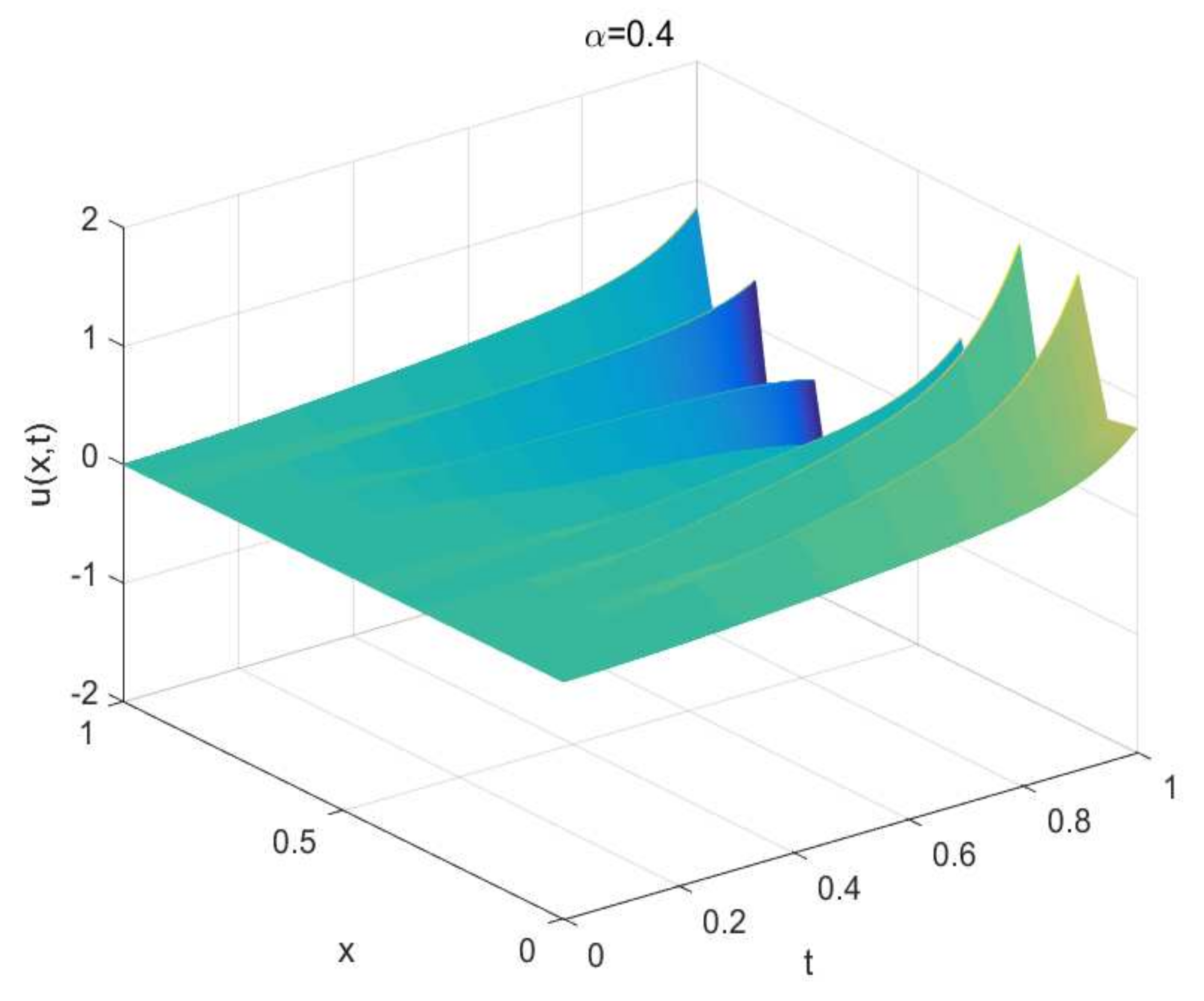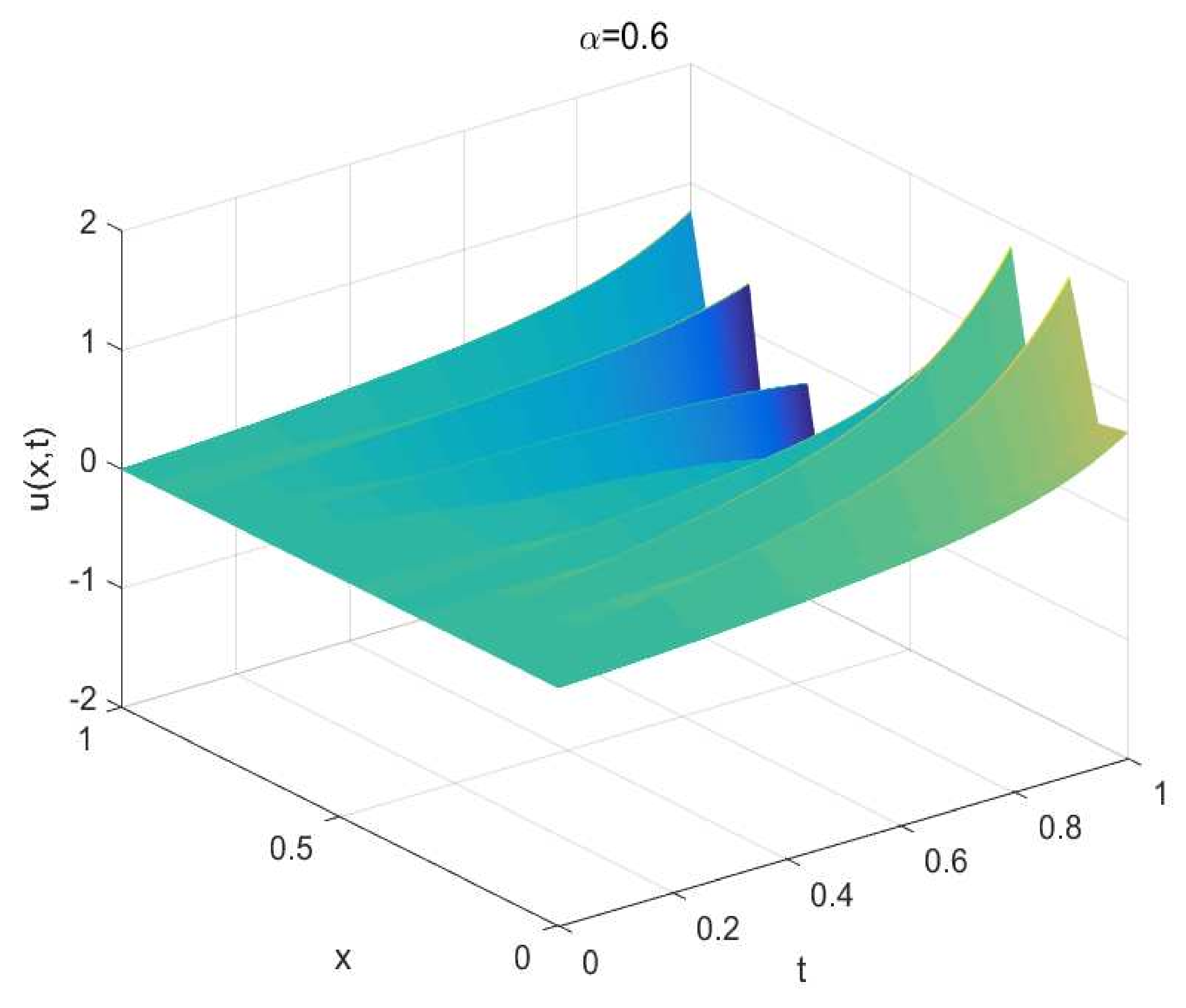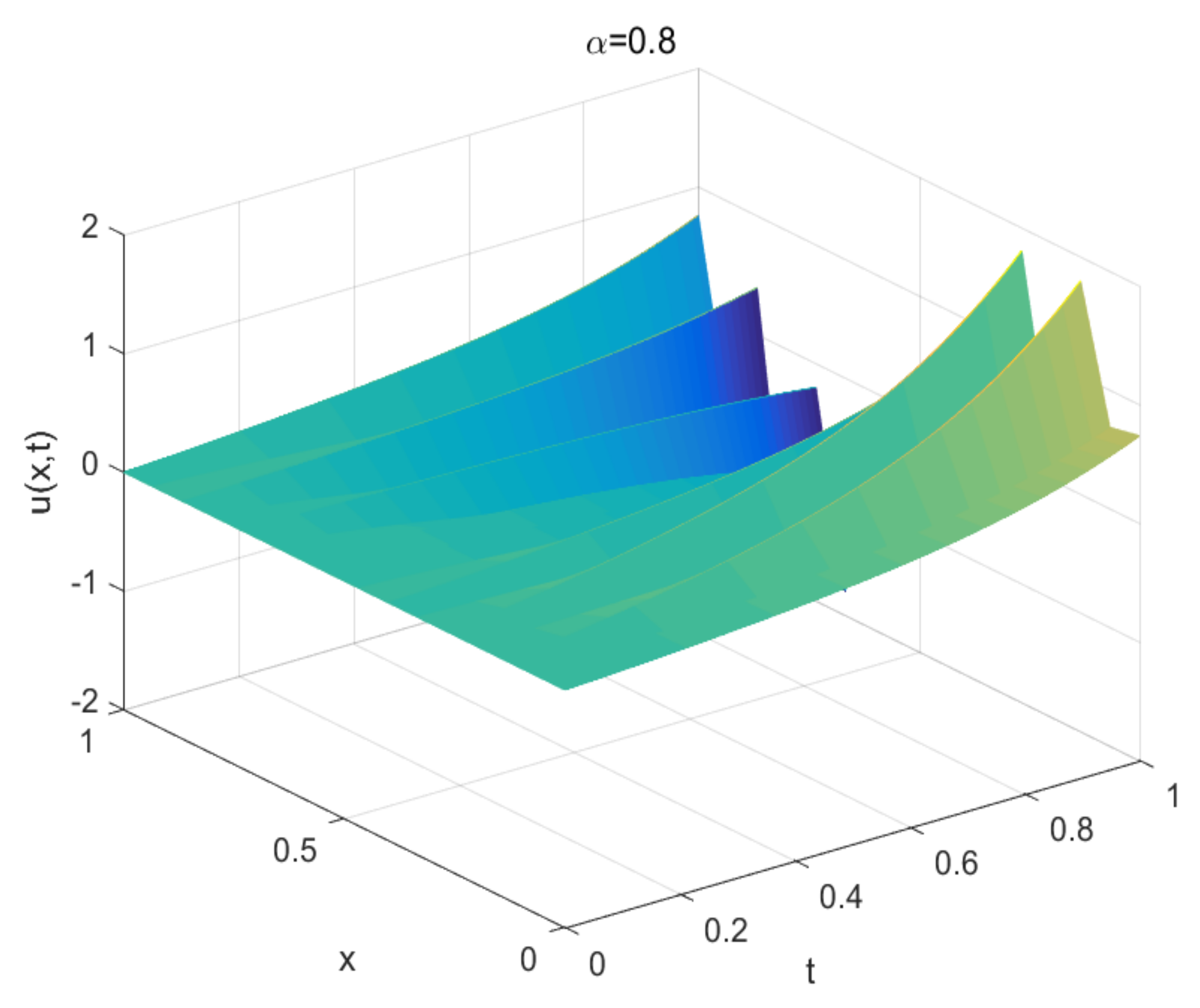In Table 2 and Table 3, for fixed $M=4000$ and $r=(2-\alpha )/\alpha$, we observe that the spatial convergence order for (18) is $(k+1)$, which is in agreement with the theoretical analysis. The numerical solutions of the scheme (18) for different $\alpha$ are given in Figure 1, Figure 2 and Figure 3. 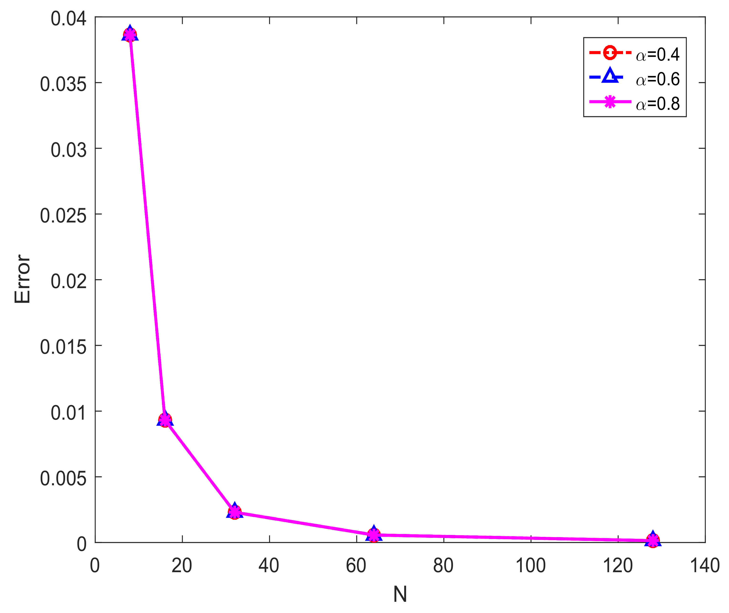Figure 4 depicts the $L^2$-norm errors versus N between the numerical solution and the exact solution for different $\alpha$ at $t=1$. The graphs show good agreement between the two solutions.

Table 1. The $L^2$-norm errors and corresponding temporal convergence orders for Example 1 with $T=1$, by the scheme (18) with $M=N$ and $r=(2-\alpha )/\alpha$.

	$\mathit{\alpha }=0.4$			$\mathit{\alpha }=0.6$			$\mathit{\alpha }=0.8$
$\mathit{M}$	Error	Order	Time(s)	Error	Order	Time(s)	Error	Order	Time(s)
320	2.24 × 10−5	*	11.79	3.16 × 10−5	*	17.26	4.11 × 10−5	*	32.11
640	7.66 × 10−6	1.55	46.20	1.75 × 10−5	0.85	60.55	2.69 × 10−5	0.61	131.45
1280	3.06 × 10−6	1.32	198.90	8.53 × 10−6	1.04	247.78	1.58 × 10−5	0.77	546.24
2560	1.14 × 10−6	1.42	1.32 × 103	3.90 × 10−6	1.13	1.05 × 103	8.96 × 10−6	0.82	2.11 × 103
5120	4.05 × 10−7	1.49	1.11 × 104	1.67 × 10−6	1.22	4.30 × 104	4.82 × 10−6	0.89	5.80 × 103

Table 2. The $L^2$-norm errors and corresponding spatial convergence orders for Example 1 with $T=1$, by the scheme (18) with $M=4000$, $r=(2-\alpha )/\alpha$ and $k=1$.

	$\mathit{\alpha }=0.4$			$\mathit{\alpha }=0.6$			$\mathit{\alpha }=0.8$
$\mathit{N}$	Error	Order	Time(s)	Error	Order	Time(s)	Error	Order	Time(s)
8	3.86 × 10−2	*	43.2	3.86 × 10−2	*	130.68	3.86 × 10−2	*	131.23
16	9.32 × 10−3	2.05	48.96	9.32 × 10−3	2.05	144.60	9.32 × 10−3	2.05	144.72
32	2.30 × 10−3	2.02	55.94	2.30 × 10−3	2.02	187.88	2.30 × 10−3	2.02	170.32
64	5.71 × 10−4	2.01	70.67	5.71 × 10−4	2.01	215.64	5.71 × 10−4	2.01	215.34
128	1.42 × 10−4	2.01	124.49	1.42 × 10−4	2.01	310.24	1.42 × 10−4	2.01	309.78

Table 3. The $L^2$-norm errors and corresponding spatial convergence orders for Example 1 with $T=1$, by the scheme (18) with $M=4000$, $r=(2-\alpha )/\alpha$ and $k=2$.

	$\mathit{\alpha }=0.4$			$\mathit{\alpha }=0.6$			$\mathit{\alpha }=0.8$
$\mathit{N}$	Error	Order	Time(s)	Error	Order	Time(s)	Error	Order	Time(s)
8	2.86 × 10−3	*	108.24	2.86 × 10−3	*	139.64	2.86 × 10−3	*	66.67
16	3.57 × 10−4	3.00	143.79	3.57 × 10−4	3.00	124.51	3.57 × 10−4	3.00	59.16
32	4.46 × 10−5	3.00	214.65	4.46 × 10−5	3.00	203.55	4.46 × 10−5	3.00	104.89
64	5.58 × 10−6	3.00	253.46	5.58 × 10−6	3.00	168.07	6.07 × 10−6	2.88	234.49

Figure 1. The numerical solution the scheme (18) for Example 1 with $\alpha =0.4$, $N=8$, $M=4000$, $r=(2-\alpha )/\alpha$ and $T=1$.

Figure 2. The numerical solution by the scheme (18) for Example 1 with $\alpha =0.6$, $N=8$, $M=4000$, $r=(2-\alpha )/\alpha$, and $T=1$.

Figure 3. The numerical solution by the scheme (18) for Example 1 with $\alpha =0.8$, $N=8$, $M=4000$, $r=(2-\alpha )/\alpha$ and $T=1$.

Figure 4. $L^2$-norm errors versus N with different values of $\alpha$, $M=4000$, $r=(2-\alpha )/\alpha$, $k=1$ and $T=1$.

Example 2.

The purpose of this example is to investigate the accuracy and efficiency of the proposed nonuniform $L2$-$1_{\sigma }$–LDG method (57). For simplicity, the equation in Example 1 is still regarded as a test problem, but it is solved by the scheme (57). The $L^2$-norm errors at time $t=1$ and convergence orders in the temporal direction with different α and r are shown in Table 4, Table 5 and Table 6. The orders of convergence displayed indicate that the order of convergence is $\mathcal{O}\left(M^{-min\{r\alpha ,2\}}\right)$, which coincides with Theorem 4. From Table 5 and Table 6, we can also see that the grading parameter $r\ge 2/\alpha$ yields the temporal optimal second-order accuracy. Then, we refine the spatial step size with a fixed temporal step size $M=2000$. The $L^2$-norm errors at time $t=1$ and convergence orders in the spatial direction are shown in Table 7. The results imply that the algorithm (57) has an accuracy of $\mathcal{O}\left(h^{k+1}\right)$ in space.

Table 4. The $L^2$-norm errors and corresponding temporal convergence orders for Example 2 with $T=1$, by the scheme (57) with $N=2000$ and $r=1$.

	$\mathit{\alpha }=0.4$			$\mathit{\alpha }=0.6$			$\mathit{\alpha }=0.8$
$\mathit{M}$	Error	Order	Time(s)	Error	Order	Time(s)	Error	Order	Time(s)
8	4.35 × 10−2	*	1.86	3.03 × 10−2	*	1.73	1.34 × 10−2	*	1.73
16	3.32 × 10−2	0.39	3.52	2.03 × 10−2	0.58	3.46	8.05 × 10−3	0.74	3.48
32	2.52 × 10−2	0.40	16.09	1.34 × 10−2	0.60	7.42	4.63 × 10−3	0.80	6.91
64	1.91 × 10−2	0.40	44.95	8.80 × 10−3	0.61	14.28	2.62 × 10−3	0.82	14.27
128	1.44 × 10−2	0.41	88.86	5.76 × 10−3	0.61	30.28	1.46 × 10−3	0.84	30.04
256	1.09 × 10−2	0.40	96.78	3.75 × 10−3	0.62	66.12	7.96 × 10−4	0.88	124.61

Table 5. The $L^2$-norm errors and corresponding temporal convergence orders for Example 2 with $T=1$, by the scheme (57) with $N=2000$ and $r=2/\alpha$.

	$\mathit{\alpha }=0.4$			$\mathit{\alpha }=0.6$			$\mathit{\alpha }=0.8$
$\mathit{M}$	Error	Order	Time(s)	Error	Order	Time(s)	Error	Order	Time(s)
8	7.31 × 10−2	*	1.76	5.78 × 10−2	*	5.15	4.38 × 10−2	*	5.23
16	2.47 × 10−2	1.57	3.53	1.66 × 10−2	1.80	10.31	1.16 × 10−2	1.92	10.38
32	7.06 × 10−3	1.81	15.48	4.41 × 10−3	1.91	20.77	2.96 × 10−3	1.97	20.87
64	1.88 × 10−3	1.91	43.15	1.13 × 10−3	1.96	42.93	7.50 × 10−4	1.98	42.60
128	4.84 × 10−4	1.96	89.74	2.87 × 10−4	1.98	89.82	1.89 × 10−4	1.99	90.16
256	1.23 × 10−4	1.98	195.20	7.26 × 10−5	1.98	197.98	4.77 × 10−5	1.99	195.35

Table 6. The $L^2$-norm errors and corresponding temporal convergence orders for Example 2 with $T=1$, by the scheme (57) with $N=2000$ and $r=(3-\alpha )/\alpha$.

	$\mathit{\alpha }=0.4$			$\mathit{\alpha }=0.6$			$\mathit{\alpha }=0.8$
$\mathit{M}$	Error	Order	Time(s)	Error	Order	Time(s)	Error	Order	Time(s)
8	9.97 × 10−2	*	1.83	7.66 × 10−2	*	5.04	5.19 × 10−2	*	5.14
16	3.77 × 10−2	1.40	3.62	2.32 × 10−2	1.72	10.19	1.40 × 10−2	1.90	10.22
32	1.14 × 10−2	1.73	17.98	6.27 × 10−3	1.89	20.05	3.58 × 10−3	1.96	20.85
64	3.11 × 10−3	1.88	37.18	1.62 × 10−3	1.95	41.64	9.06 × 10−4	1.98	42.06
128	8.08 × 10−4	1.94	89.39	4.12 × 10−4	1.98	88.55	2.28 × 10−4	1.99	88.94
256	2.06 × 10−4	1.97	175.39	1.04 × 10−4	1.99	169.03	5.76 × 10−5	1.98	109.57

Table 7. The $L^2$-norm errors and corresponding spatial convergence orders for Example 2 with $T=1$, by the scheme (57) with $M=2000$, $r=(3-\alpha )/\alpha$ and $k=1$.

	$\mathit{\alpha }=0.4$			$\mathit{\alpha }=0.6$			$\mathit{\alpha }=0.8$
$\mathit{N}$	Error	Order	Time(s)	Error	Order	Time(s)	Error	Order	Time(s)
8	3.86 × 10−2	*	975.25	3.86 × 10−2	*	1.22 × 103	3.86 × 10−2	*	1.73 × 103
16	9.32 × 10−3	2.05	969.18	9.32 × 10−3	2.05	1.16 × 103	9.32 × 10−3	2.05	689.66
32	2.30 × 10−3	2.02	939.20	2.30 × 10−3	2.02	1.70 × 103	2.30 × 10−3	2.02	686.89
64	5.74 × 10−4	2.00	945.52	5.72 × 10−4	2.01	1.82 × 103	5.72 × 10−4	2.01	733.29
128	1.46 × 10−4	1.97	1.44 × 103	1.44 × 10−4	1.99	2.63 × 103	1.43 × 10−4	2.00	761.07
256	3.90 × 10−5	1.90	4.71 × 103	3.72 × 10−5	1.95	1.45 × 103	3.65 × 10−5	1.97	800.52

6. Concluding Remarks

In this paper, we studied the numerical algorithms for the time-fractional fourth-order equation with an initial singularity. In the temporal direction, two types of finite difference schemes were proposed and analyzed, including the nonuniform L1 scheme and nonuniform $L2$-$1_{\sigma }$ scheme. In the spatial direction, the LDG method was utilized. Detailed proofs of $L^2$ stability and optimal error estimates for the schemes were derived using the discrete fractional Gronwall-type inequalities. Finally, some numerical examples were presented to verify the theoretical results.

References

1. Li, C.P.; Cai, M. Theory and Numerical Approximations of Fractional Integrals and Derivatives; SIAM: Philadelphia, PA, USA, 2019. [Google Scholar]
2. Podlubny, I. Fractional Differential Equations; Academic Press: New York, NY, USA, 1999. [Google Scholar]
3. Du, Y.; Liu, Y.; Li, H.; Fang, Z.; He, S. Local discontinuous Galerkin method for a nonlinear time-fractional fourth-order partial differential equation. J. Comput. Phys. 2017, 344, 108–126. [Google Scholar] [CrossRef]
4. Ji, C.; Sun, Z.; Hao, Z. Numerical algorithms with high spatial accuracy for the fourth-order fractional sub-diffusion equations with the first Dirichlet boundary conditions. J. Sci. Comput. 2015, 3, 1148–1174. [Google Scholar] [CrossRef]
5. Zhang, H.; Yang, X.; Xu, D. A high-order numerical method for solving the 2D fourth-order reaction-diffusion equation. Numer. Algor. 2019, 80, 849–877. [Google Scholar] [CrossRef]
6. Wei, L.; He, Y. Analysis of a fully discrete local discontinuous Galerkin method for time-fractional fourth-order problems. Appl. Math. Model. 2014, 38, 1511–1522. [Google Scholar] [CrossRef]
7. Guo, L.; Wang, Z.; Vong, S. Fully discrete local discontinuous Galerkin methods for some time-fractional fourth-order problems. Int. J. Comput. Math. 2016, 93, 1665–1682. [Google Scholar] [CrossRef]
8. Liu, Y.; Fang, Z.; Li, H.; He, S. A mixed finite element method for a time-fractional fourth-order partial differential equation. Appl. Math. Comput. 2014, 243, 703–717. [Google Scholar] [CrossRef]
9. Zhang, P.; Pu, H. A second-order compact difference scheme for the fourth-order fractional sub-diffusion equation. Numer. Algor. 2017, 76, 573–598. [Google Scholar] [CrossRef]
10. Cui, M. Compact difference scheme for time-fractional fourth-order equation with first Dirichlet boundary condition. East Asian J. Appl. Math. 2019, 9, 45–66. [Google Scholar] [CrossRef]
11. Fei, M.; Huang, C. Galerkin-Legendre spectral method for the distributed-order time fractional fourth-order partial differential equation. Int. J. Comput. Math. 2019, 97, 1183–1196. [Google Scholar] [CrossRef]
12. Fakhar-Izadi, F. Fully spectral-Galerkin method for the one- and two-dimensional fourth-order time-fractional partial integro-differential equations with a weakly singular kernel. Numer. Methods Partial Differ. Equ. 2022, 38, 160–176. [Google Scholar] [CrossRef]
13. Hosseini, V.R.; Koushki, M.; Zou, W.N. The meshless approach for solving 2D variable-order time-fractional advection-diffusion equation arising in anomalous transport. Eng. Comput. 2021. [Google Scholar] [CrossRef]
14. Huang, C.; Stynes, M.; An, N. Optimal L(L2) error analysis of a direct discontinuous Galerkin method for a time-fractional reaction-diffusion problem. BIT Numer. Math. 2018, 58, 661–690. [Google Scholar] [CrossRef]
15. Jin, B.; Lazarov, R.; Zhou, Z. Numerical methods for time-fractional evolution equations with nonsmooth data: A concise overview. Comput. Methods Appl. Mech. Engrg. 2019, 346, 332–358. [Google Scholar] [CrossRef] [Green Version]
16. Kopteva, N. Error analysis of the L1 method on graded and uniform meshes for a fractional-derivative problem in two and three dimensions. Math. Comp. 2019, 88, 2135–2155. [Google Scholar] [CrossRef]
17. Li, C.P.; Li, D.X.; Wang, Z. L1/LDG method for the generalized time-fractional Burgers equation. Math. Comput. Simulat. 2021, 187, 357–378. [Google Scholar] [CrossRef]
18. Li, C.P.; Wang, Z. Numerical methods for the time fractional convection-diffusion-reaction equation. Numer. Func. Anal. Opt. 2021, 42, 1115–1153. [Google Scholar] [CrossRef]
19. Liao, H.; Li, D.; Zhang, J. Sharp error estimate of nonuniform L1 formula for linear reaction-subdiffusion equations. SIAM J. Numer. Anal. 2018, 56, 1112–1133. [Google Scholar] [CrossRef]
20. Lyu, P.; Vong, S. Second-order and nonuniform time-stepping schemes for time fractional evolution equations with time-space dependent coefficients. J. Sci. Comput. 2021, 89, 49. [Google Scholar] [CrossRef]
21. Nikan, O.; Avazzadeh, Z.; Machado, J.A.T. Numerical study of the nonlinear anomalous reaction-subdiffusion process arising in the electroanalytical chemistry. J. Comput. Sci. 2021, 53, 101394. [Google Scholar] [CrossRef]
22. Stynes, M.; O’Riordan, E.; Gracia, J.L. Error analysis of a finite difference method on graded mesh for a time-fractional diffusion equation. SIAM J. Numer. Anal. 2017, 55, 1057–1079. [Google Scholar] [CrossRef]
23. Wang, H.; Zhang, Q.; Shu, C.-W. Stability analysis and error estimates of local discontinuous Galerkin methods with implicit-explicit time-marching for the time-dependent fourth order PDEs. ESAIM Math. Model. Numer. Anal. 2017, 51, 1931–1955. [Google Scholar] [CrossRef]
24. Dong, B.; Shu, C.-W. Analysis of a local discontinuous Galerkin methods for linear time-dependent fourth-order problems. SIAM J. Numer. Anal. 2009, 47, 3240–3268. [Google Scholar] [CrossRef]
25. Ren, J.; Liao, H.; Zhang, J.; Zhang, Z. Sharp H1-norm error estimates of two time-stepping schemes for reaction-subdiffusion problems. J. Comput. Appl. Math. 2021, 389, 113352. [Google Scholar] [CrossRef]
26. Alikhanov, A. A new difference scheme for the time fractional diffusion equation. J. Comput. Phys. 2015, 280, 424–438. [Google Scholar] [CrossRef] [Green Version]
27. Wang, H.; Shu, C.-W.; Zhang, Q. Stability and error estimates of the local discontinuous Galerkin method with implicit-explicit time-marching for nonlinear convection-diffusion problems. Appl. Math. Comput. 2015, 272, 237–258. [Google Scholar] [CrossRef] [Green Version]
28. Liao, H.; McLean, W.; Zhang, J. A second-order scheme with nonuniform time steps for a linear reaction-subdiffusion problem. Commun. Comput. Phys. 2021, 30, 567–601. [Google Scholar] [CrossRef]
29. Liao, H.; McLean, W.; Zhang, J. A discrete Gronwall inequality with applications to numerical schemes for subdiffusion problems. SIAM J. Numer. Anal. 2019, 57, 218–237. [Google Scholar] [CrossRef]
30. Chen, H.; Stynes, M. Error analysis of a second-order method on fitted meshes for a time-fractional diffusion problem. J. Sci. Comput. 2019, 79, 624–647. [Google Scholar] [CrossRef]