Semi-Analytical Solutions for Fuzzy Caputo–Fabrizio Fractional-Order Two-Dimensional Heat Equation

Abstract

In the analysis in this article, we developed a scheme for the computation of a semi-analytical solution to a fuzzy fractional-order heat equation of two dimensions having some external diffusion source term. For this, we applied the Laplace transform along with decomposition techniques and the Adomian polynomial under the Caputo–Fabrizio fractional differential operator. Furthermore, for obtaining a semi-analytical series-type solution, the decomposition of the unknown quantity and its addition established the said solution. The obtained series solution was calculated and approached the approximate solution of the proposed equation. For the validation of our scheme, three different examples have been provided, and the solutions were calculated in fuzzy form. All the three illustrations simulated two different fractional orders between 0 and 1 for the upper and lower portions of the fuzzy solution. The said fractional operator is nonsingular and global due to the presence of the exponential function. It globalizes the dynamical behavior of the said equation, which is guaranteed for all types of fuzzy solution lying between 0 and 1 at any fractional order. The fuzziness is also included in the unknown quantity due to the fuzzy number providing the solution in fuzzy form, having upper and lower branches.

1. Introduction

The area of fractional calculus has attained considerable attention in the last three decades. Famous scientists have provided their contributions on this aspect by introducing different fractional operators in different articles. Modern calculus has provided more realistic results than classical calculus. It has described the dynamics of different real-world phenomena lying between two integers. Furthermore, the fractional operators have more degrees of freedom, and they generalize the integer differential operators. To date, various researchers have published more research articles, more books and different monographs that touch upon the said area. Podlubny provides a physical and geometrical explanation of the fractional-order derivatives [1]. An analysis of various dynamical systems in the sense of fractional-order operators can be seen in [2]. The applications of the said calculus in physics may be studied in [3]. Some fuzzy fractional-order linear and non-linear dynamical problems have been analyzed for semi-analytical solutions using fractional Sumudo transform [4,5]. Many types of publications have also been based on existence, uniqueness and numerical analysis under fractional-order concepts.

Modern calculus can be extended to various fields of physical and natural sciences. These operators may be applicable in the field of applied and pure mathematics. Now, we will apply these operators to those fields where fuzziness lies in the data. Uncertainty may be found in quantum mechanics, chemistry and different distributions of chromosomes in humans or other living things. The concepts of fuzziness were first introduced by Zadeh [6] in 1965 for sets by defining the membership function. The idea of uncertainty was then applied in other areas, i.e., fuzzy topology, the fixed-point theorem, fuzzy automata, control systems, etc. Zadeh, Chang and a few other scientists have applied this idea of fuzzy sets to define some membership functions and fuzzy control [7]. By applying the idea of fuzziness and its operators, various scholars have published basic fuzzy differential calculus [8]. Elementary fuzzy calculus and the study of fuzzy differential equations may be seen in [9,10]. From 2001, differential equations have been presented in fuzzy form by taking account of uncertainty in the initial data. Some scholars such as “Dobius” and “Prada” have defined the fundamental concepts of integral equations in fuzzy form [11]. We deal with all those problems having uncertainty or vagueness in their information using fuzzy differential and integral equations or systems. Therefore, plenty of research work on such types of fuzzy fractional differential equations (FDEs) has been presented by many researchers [12,13,14].

Semi-analytical investigations for the solution of fuzzy FDEs, important techniques and schemes have been introduced in the past. Among them are the well-known integral transforms of Fourier, Natural, Z, Laplace, Sumudu, etc. [4,15,16]. Some of the iterative and series solution methods such as the “homotopy and improved homotopy method” [17,18,19], Adomian decomposition along with Adomian polynomial and Laplace Adomian decomposition methods (LADM) [20,21], “Taylor’s” series method, etc. have also been used for dealing with such problems [22,23]. However, to the best of our knowledge, the aforementioned techniques have not been properly used to study fuzzy fractional partial differential equations (FPDEs). The idea of a nonsingular fractional derivative is new and has very recently received attention. Here, we remark that, recently, some valuable work related to applications of the nonsingular kernel type derivatives CF and ABC have been considered; see [24,25,26,27,28,29].

As far as novelty is concerned, we consider an initial value heat equation with external source terms under the fuzzy Caputo fractional operator. We take the fuzziness in an unknown quantity and initial conditions to find its approximate solution in fuzzy form with two branches, because of the fuzzy number. Different scientists have worked on diffusion equations, of both integer and fractional order; some have worked on the fuzzy heat equation. We consider both fuzziness and fractional order for the analysis of the said equation having different external source terms [12,13,14,30,31,32]. Therefore, a fuzzy solution is required, as many quantities can be obtained in fuzzy format when there is some ambiguity regarding the exact quantity. Keep in mind the fact that the considered method has the ability to produce series-type solutions for such problems under consideration. Furthermore, this method decreases the error and avoids wasting time. Additionally, this method is free from any axillary parameters that run the whole system. The adopted method can be used as a robust tool to analyze fuzzy problems under the mentioned fractional operator. Therefore, here, in the current work, we compute a semi-analytical series solution or approximate solution using analytical techniques applying Laplace Adomian decomposition under the fuzzy Caputo–Fabrizio derivative concept for the proposed 2D heat equation given as

$$\begin{array}{ccc}\hfill {}^{CF}{\mathcal{D}}_{\tau }^{\theta }\tilde{\mathrm{U}}(x_1,x_2,\tau )& =& {\mathcal{D}}_{x_1}^2\tilde{\mathrm{U}}(x_1,x_2,\tau )+{\mathcal{D}}_{x_2}^2\tilde{\mathrm{U}}(x_1,x_2,\tau )+\mathcal{F}(x_1,x_2,\tau )\tilde{\mathrm{k}}\left(r\right),0<\theta \le 1,\hfill \\ \hfill \tilde{\mathrm{U}}(x_1,x_2,0)& =& \tilde{k}\left(r\right)g(x_1,x_2),\hfill \end{array}$$

(1)

where ${}^{CF}{\mathcal{D}}_{\tau }^{\theta }$ represents the Caputo–Fabrizio fractional operator while

$$\mathcal{F}\in C({\mathcal{R}}^3,\mathcal{R}),\tilde{g}\in \left({\mathcal{R}}^3\right).$$

Generally, the transfer of heat in a thin rod from one point to the other can be formulated by the boundary value problem of the one-dimensional heat equation. The two-dimensional heat equation represents the transfer of heat through an infinite thin sheet. Here, $\tilde{\mathrm{U}}$ represents the temperature of the body at any point in the thin sheet. The phenomena of heat transfer may be found in many diffusion problems. Therefore, the investigation of partial differential equations such as the heat equation has much more application in real life [33,34]. The analysis for semi-analytical solutions for the problems of electrical circuits [35] has been performed using numerical approximation. The use of different analytical techniques such as Laplace transform may be found in [36]. The technique of double Laplace transform for waves and Laplace equations was conducted in [37]. The phenomenon of heat conduction was discussed in [38]. The semi-analytical solution, via the Laplace Adomian decomposition method, is provided in [39,40]. The semi-analytical solution of the 2D heat equation was found using double Laplace transform without an external diffusion term $\mathcal{F}$ in [37]. We analyze the 2D heat equation by applying the external term under the fuzzy concept. Different examples along with a numerical simulation were used to perform the verification of the theoretical results.

2. Background Materials

In the following part, we present some theorems, lemmas and definitions of classical calculus [1,2] and some well-known fractional operators from [11,41].

Definition 1.

Take a continuous fuzzy operator $\tilde{\mathrm{U}}\left(\tau \right)$ on a $[0,b]$ subset of $\mathcal{R};$ we provide the definition of fuzzy fractional-order integration in Caputo–Fabrizio type w.r.t τ as

$$\begin{array}{c}\hfill {}^{CF}{\mathbf{I}}^{\theta }\tilde{\mathrm{U}}\left(\tau \right)=\frac{1-\theta }{M\left(\theta \right)}\tilde{\mathrm{U}}\left(\tau \right)+\frac{\theta }{M\left(\theta \right)}{\int }_0^{\tau }\tilde{\mathrm{U}}\left(\eta \right)d\eta ,\theta ,\eta \in (0,\infty ),\end{array}$$

(2)

where $M\left(0\right)=M\left(1\right)=1$. Next, if $\widetilde{\mathrm{U}\left(\tau \right)}\in L^F[0,b]\cap C^F[0,b]$, $C^F[0,b]$ is the space of the fuzzy operator along with continuity while $L^F[0,b]$ is the space of Lebesgue fuzzy integrable operators, respectively, then the non-integer-order Caputo–Fabrizio fuzzy integration is given as:

$$\begin{array}{c}\hfill {{[}^{CF}{\mathbf{I}}^{\theta }\tilde{\mathrm{U}}\left(\tau \right)]}_r=[{\mathbf{I}}^{\theta }{\underline{\mathrm{U}}}_r\left(\tau \right),{\mathbf{I}}^{\theta }{\overline{\mathrm{U}}}_r\left(\tau \right)],0\le r\le 1,\end{array}$$

(3)

or

$$\begin{array}{c}\hfill {}^{CF}{\mathbf{I}}^{\theta }\underline{\mathrm{U}}\left(\tau \right)=\frac{1-\theta }{M\left(\theta \right)}\underline{\mathrm{U}}\left(\tau \right)+\frac{\theta }{M\left(\theta \right)}{\int }_0^{\tau }\underline{\mathrm{U}}\left(\eta \right)d\eta ,\theta ,\eta \in (0,\infty ).\\ \hfill {}^{CF}{\mathbf{I}}^{\theta }\overline{\mathrm{U}}\left(\tau \right)=\frac{1-\theta }{M\left(\theta \right)}\overline{\mathrm{U}}\left(\tau \right)+\frac{\theta }{M\left(\theta \right)}{\int }_0^{\tau }\overline{\mathrm{U}}\left(\eta \right)d\eta ,\theta ,\eta \in (0,\infty ).\end{array}$$

Definition 2.

Similarly, for an operator $\tilde{\mathrm{U}}\left(\tau \right)\in L^F[0,b]\cap C^F[0,b]$, as $\tilde{\mathrm{U}}\left(\tau \right)=[{\underline{U}}_r\left(\tau \right),{\overline{U}}_r\left(\tau \right)],$$0\le r\le 1$ and $0<{\tau }_0<b,$ the fractional-order Caputo–Fabrizio (CF) differential operator in the fuzzy sense is given as

$$\begin{array}{ccc}\hfill {{[}^{CF}{\mathcal{D}}^{\theta }\tilde{\mathrm{U}}\left({\tau }_0\right)]}_r& =& [{\mathcal{D}}^{\theta }{\underline{\mathrm{U}}}_r\left({\tau }_0\right),{\mathcal{D}}^{\theta }{\overline{\mathrm{U}}}_r\left({\tau }_0\right)],0<\theta \le 1,\hfill \end{array}$$

(4)

here

$$\begin{array}{ccc}\hfill {}^{CF}{\mathcal{D}}^{\theta }{\underline{\mathrm{U}}}_r\left({\tau }_0\right)& =& \frac{M\left(\theta \right)}{1-\theta }\left[{\int }_0^{\tau }\underline{{\mathrm{U}}^{\prime }}\left(\eta \right)exp\left(\frac{-\theta (\tau -\eta )}{1-\theta }\right)d\eta \right],\hfill \\ \hfill {}^{CF}{\mathcal{D}}^{\theta }{\overline{\mathrm{U}}}_r\left({\tau }_0\right)& =& \frac{M\left(\theta \right)}{1-\theta }\left[{\int }_0^{\tau }\overline{{\mathrm{U}}^{\prime }}\left(\eta \right)exp\left(\frac{-\theta (\tau -\eta )}{1-\theta }\right)d\eta \right],\hfill \end{array}$$

where the integration exists or converges and $m=\lceil \theta \rceil +1$. As θ lies in the interval (0, 1], $m=1$.

Definition 3.

For x, either real or complex, the transform of Laplace for the fuzzy function $\mathcal{F}\left(x\right)$ is given as

$$\mathcal{F}\left(x\right)=L\left[f\left(x\right)\right]={\int }_0^{\infty }{e}^{-x\tau }f\left(\tau \right)d\tau \tau >0.$$

(5)

Definition 4.

The Laplace transform for CF is

$$\begin{array}{c}\hfill L{[}^{CF}{\mathcal{D}}^{\theta +n}\tilde{U}\left(t\right)]=\frac{s^{n+1}\tilde{U}\left(s\right)-s^n\tilde{U}\left(0\right)-s^{n-1}\widetilde{U^{\prime }}\left(0\right)\dots -{\tilde{U}}^n\left(0\right)}{s+\theta (1-s)}.\end{array}$$

Definition 5.

The “Mittag-Leffler” operator $E_{\beta }\left(t\right)$ is

$$E_{\beta }\left(\tau \right)=\sum _{n=0}^{\infty }\frac{{\tau }^n}{\Gamma (1+n\beta )},$$

(6)

where $0<\beta$.

Definition 6.

A mapping $k:\mathcal{R}\to [0,1]$ is called a fuzzy number if the following conditions hold:

(i)

k is continuous up to a peak value;

(ii) 

k $\left\{\mu \left(y_1\right)+\mu \left(y_2\right)\right\}\ge min\{k\left(y_1\right),k\left(y_2\right)\}$;

(iii) 

∃$y_0$∈$\mathcal{R}$; $k\left(y_0\right)=1$, i.e., k is normal;

(iv) 

$cl\{y\in \mathcal{R}$, $k\left(y\right)>0\}$ is bounded and continuous, where $cl$ represents closure for the support of y.

We denote the set of fuzzy numbers collectively as $\mathcal{E}$.

Definition 7.

The parameterization form of a “fuzzy number" is $\left(\underline{k}\left(r\right)\right),\overline{k}\left(r\right))$, for $0\le r\le 1$, and the following conditions hold:

(i) 

$\underline{k}\left(r\right)$ is left-defined on [0,1], with a bounded increasing operator on $(0,1]$;

(ii) 

$\overline{k}\left(r\right)$ is right-defined on [0,1], with a bounded decreasing operator on $(0,1]$;

(iii) 

$\overline{k}\left(r\right)\ge \underline{k}\left(r\right)$.

If $\underline{k}\left(r\right)=\overline{k}\left(r\right)=r,$ then r is the crisp number.

3. Main Work

In this section, we investigate our proposed model for a semi-analytical solution. For this, we use the Laplace transform of the Caputo–Fabrizio fractional differential operator along with decomposition techniques for (1) as

$$\begin{array}{ccc}\hfill \mathcal{L}{[}^{CF}{\mathcal{D}}_{\tau }^{\theta }\tilde{\mathrm{U}}(\tau ,x_2,x_2)]& =& \mathcal{L}\left[{\mathcal{D}}_{x_1}^2\tilde{\mathrm{U}}(\tau ,x_2,x_1)+{\mathcal{D}}_{x_2}^2\tilde{\mathrm{U}}(\tau ,x_2,x_1)+\tilde{k}\left(r\right)\mathcal{F}(\tau ,x_2,x_1)\right],\hfill \end{array}$$

(7)

where $\theta$ is in $(0,1]$; therefore, the Laplace transform of (7) is

$$\begin{array}{ccc}\hfill \frac{s\mathcal{L}\left[\tilde{\mathrm{U}}(\tau ,{\mathrm{x}}_2,{\mathrm{x}}_1)\right]-\tilde{U}(0,x_2,x_1)}{s+\theta (1-s)}& =& \mathcal{L}[{\mathcal{D}}_{x_1}^2\tilde{\mathrm{U}}(\tau ,{\mathrm{x}}_2,{\mathrm{x}}_1)+{\mathcal{D}}_{x_2}^2\tilde{\mathrm{U}}(\tau ,{\mathrm{x}}_2,{\mathrm{x}}_1)+\tilde{\mathrm{k}}\left(\mathrm{r}\right)\mathcal{F}(\tau ,{\mathrm{x}}_2,{\mathrm{x}}_1)],\hfill \end{array}$$

On using the initial condition, we obtain

$$\begin{array}{ccc}\hfill s\mathcal{L}\left[\tilde{\mathrm{U}}(\tau ,{\mathrm{x}}_2,{\mathrm{x}}_1)\right]& =& g(x_2,x_1)+(s+\theta (1-s))\mathcal{L}[{\mathcal{D}}_{x_1}^2\mathrm{u}(\tau ,x_2,x_1)+{\mathcal{D}}_{x_2}^2\mathrm{u}(\tau ,x_2,x_1)+\tilde{k}\left(r\right)\mathcal{F}(\tau ,x_2,x_1)],\hfill \\ \hfill \mathcal{L}\left[\tilde{\mathrm{U}}(\tau ,{\mathrm{x}}_2,{\mathrm{x}}_1)\right]& =& \frac{g(x_2,x_1)}{s}+\hfill \\ & & \left(\frac{s+\theta (1-s)}{s}\right)\mathcal{L}\left[{\mathcal{D}}_{x_1}^2\tilde{\mathrm{U}}(\tau ,{\mathrm{x}}_2,{\mathrm{x}}_1)+{\mathcal{D}}_{x_2}^2\tilde{\mathrm{U}}(\tau ,{\mathrm{x}}_2,{\mathrm{x}}_1)+\tilde{k}\left(r\right)\mathcal{F}(\tau ,x_2,x_1)\right].\hfill \end{array}$$

(8)

Decompose the solution as $\tilde{\mathrm{U}}(\tau ,x_2,x_1)={\sum }_{n=0}^{\infty }{\tilde{\mathrm{U}}}_n(\tau ,x_2,x_1)$; then, (8) implies

$$\begin{array}{ccc}\hfill \mathcal{L}\left[\sum _{n=0}^{\infty }{\tilde{\mathrm{U}}}_n(\tau ,x_2,x_1)\right]& =& \frac{g(x_2,x_1)}{s}+\left(\frac{s+\theta (1-s)}{s}\right)\mathcal{L}[{\mathcal{D}}_{x_1}^2\sum _{n=0}^{\infty }{\tilde{\mathrm{U}}}_n(\tau ,x_2,x_1)+\hfill \\ & & \sum _{n=0}^{\infty }{\tilde{\mathrm{U}}}_n(\tau ,x_2,x_1)+\tilde{k}\left(r\right)\mathcal{F}(\tau ,x_2,x_1)].\hfill \end{array}$$

(9)

Take parts of the solution by choice of comparison as

$$\begin{array}{ccc}\hfill \mathcal{L}\left[{\tilde{\mathrm{U}}}_0(\tau ,x_2,x_1)\right]& =& \frac{g(x_2,x_1)}{s}+\left(\frac{s+\theta (1-s)}{s}\right)\mathcal{L}\left[\tilde{k}\left(r\right)\mathcal{F}(\tau ,x_2,x_1)\right],\hfill \\ \hfill \mathcal{L}\left[{\tilde{\mathrm{U}}}_1(\tau ,x_2,x_1)\right]& =& \left(\frac{s+\theta (1-s)}{s}\right)\mathcal{L}\left[{\mathcal{D}}_{x_1}^2{\tilde{U}}_0(\tau ,x_2,x_1)+{\mathcal{D}}_{x_2}^2{\tilde{\mathrm{U}}}_0(\tau ,x_2,x_1)\right],\hfill \\ \hfill \mathcal{L}\left[{\tilde{\mathrm{U}}}_2(\tau ,x_2,x_1)\right]& =& \left(\frac{s+\theta (1-s)}{s}\right)\mathcal{L}\left[{\mathcal{D}}_{x_1}^2{\tilde{U}}_1(\tau ,x_2,x_1)+{\mathcal{D}}_{x_2}^2{\tilde{\mathrm{U}}}_1(\tau ,x_2,x_1)\right],\hfill \\ \hfill ⋮\\ \hfill \mathcal{L}\left[{\tilde{\mathrm{U}}}_{n+1}(\tau ,x_2,x_1)\right]& =& \left(\frac{s+\theta (1-s)}{s}\right)\mathcal{L}\left[{\mathcal{D}}_{x_1}^2{\tilde{U}}_n(\tau ,x_2,x_1)+{\mathcal{D}}_{x_2}^2{\tilde{\mathrm{U}}}_n(\tau ,x_2,x_1)\right].\hfill \end{array}$$

(10)

Taking the inverse Laplace transform, we obtain

$$\begin{array}{ccc}\hfill {\underline{\mathrm{U}}}_0(\tau ,x_2,x_1)& =& g(x_2,x_1)+{\mathcal{L}}^{-1}\left[\left(\frac{s+\theta (1-s)}{s}\right)\mathcal{L}\left[\underline{k}\left(r\right)\mathcal{F}(\tau ,x_2,x_1)\right]\right],\hfill \\ \hfill {\overline{\mathrm{U}}}_0(\tau ,x_2,x_1)& =& g(x_2,x_1)+{\mathcal{L}}^{-1}\left[\left(\frac{s+\theta (1-s)}{s}\right)\mathcal{L}\left[\overline{k}\left(r\right)\mathcal{F}(\tau ,x_2,x_1)\right]\right],\hfill \\ \hfill {\underline{\mathrm{U}}}_1(\tau ,x_2,x_1)& =& {\mathcal{L}}^{-1}\left[\left(\frac{s+\theta (1-s)}{s}\right)\mathcal{L}[{\mathcal{D}}_{x_1}^2{\underline{\mathrm{U}}}_0(\tau ,x_2,x_1)+{\mathcal{D}}_{x_2}^2{\underline{\mathrm{U}}}_0(\tau ,x_2,x_1)]\right],\hfill \\ \hfill {\overline{\mathrm{U}}}_1(\tau ,x_2,x_1)& =& {\mathcal{L}}^{-1}\left[\left(\frac{s+\theta (1-s)}{s}\right)\mathcal{L}[{\mathcal{D}}_{x_1}^2{\overline{\mathrm{U}}}_0(\tau ,x_2,x_1)+{\mathcal{D}}_{x_2}^2{\overline{\mathrm{U}}}_0(\tau ,x_2,x_1)]\right],\hfill \\ \hfill {\underline{\mathrm{U}}}_2(\tau ,x_2,x_1)& =& {\mathcal{L}}^{-1}\left[\left(\frac{s+\theta (1-s)}{s}\right)\mathcal{L}[{\mathcal{D}}_{x_1}^2{\underline{\mathrm{U}}}_1(\tau ,x_2,x_1)+{\mathcal{D}}_{x2}^2{\underline{\mathrm{U}}}_1(\tau ,x_2,x_1)]\right],\hfill \\ \hfill {\overline{\mathrm{U}}}_2(\tau ,x_2,x_1)& =& {\mathcal{L}}^{-1}\left[\left(\frac{s+\theta (1-s)}{s}\right)\mathcal{L}[{\mathcal{D}}_{x_1}^2{\overline{\mathrm{U}}}_1(\tau ,x_2,x_1)+{\mathcal{D}}_{x_2}^2{\overline{\mathrm{U}}}_1(\tau ,x_2,x_1)]\right],\hfill \\ \hfill ⋮\\ \hfill {\underline{\mathrm{U}}}_{n+1}(\tau ,x_2,x_1)& =& {\mathcal{L}}^{-1}\left[\left(\frac{s+\theta (1-s)}{s}\right)\mathcal{L}[{\mathcal{D}}_{x_1}^2{\underline{\mathrm{U}}}_n(\tau ,x_2,x_1)+{\mathcal{D}}_{x_2}^2{\underline{\mathrm{U}}}_n(\tau ,x_2,x_1)]\right],\hfill \\ \hfill {\overline{\mathrm{U}}}_{n+1}(\tau ,x_2,x_1)& =& {\mathcal{L}}^{-1}\left[\left(\frac{s+\theta (1-s)}{s}\right)\mathcal{L}[{\mathcal{D}}_{x_1}^2{\overline{\mathrm{U}}}_n(\tau ,x_2,x_1)+{\mathcal{D}}_{x_2}^2{\overline{\mathrm{U}}}_n(\tau ,x_2,x_1)]\right],\hfill \\ \hfill n\ge 0.\end{array}$$

(11)

Thus, the solution becomes

$$\begin{array}{ccc}\hfill \underline{\mathrm{U}}(\tau ,x_2,x_1)& =& {\underline{\mathrm{U}}}_0(\tau ,x_2,x_1)+{\underline{\mathrm{U}}}_1(\tau ,x_2,x_1)+{\underline{\mathrm{U}}}_2(\tau ,x_2,x_1)+\cdots ,\hfill \\ \hfill \overline{\mathrm{U}}(\tau ,x_2,x_1)& =& {\overline{\mathrm{U}}}_0(\tau ,x_2,x_1)+{\overline{\mathrm{U}}}_1(\tau ,x_2,x_1)+{\overline{\mathrm{U}}}_2(\tau ,x_2,x_1)+\cdots .\hfill \end{array}$$

(12)

Equation (12) is the solution in series form, whose convergence was also derived in [42].

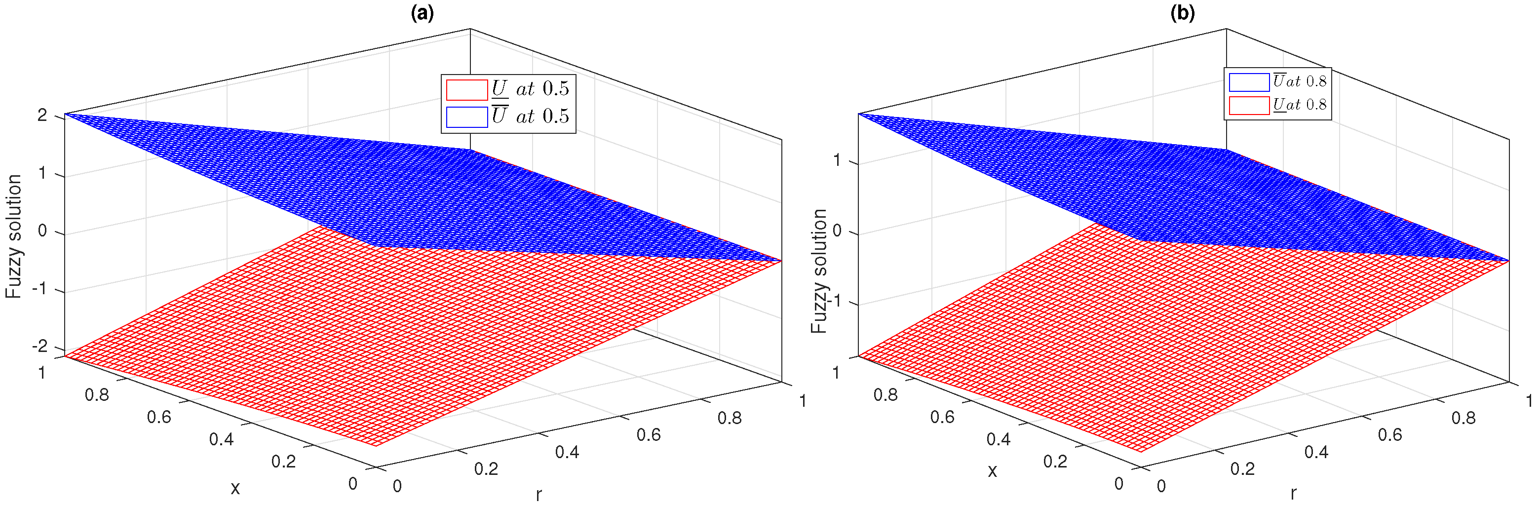
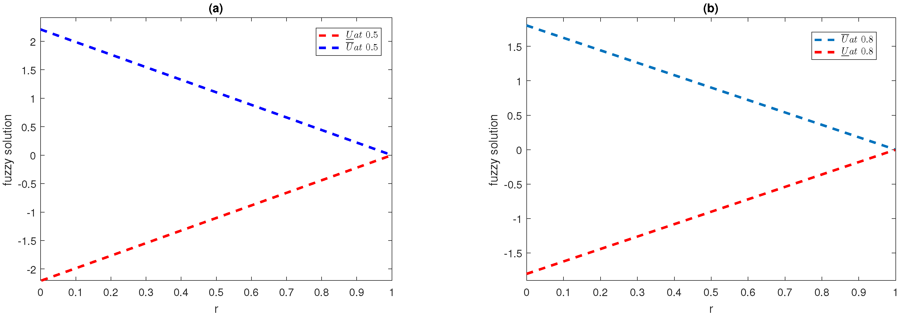
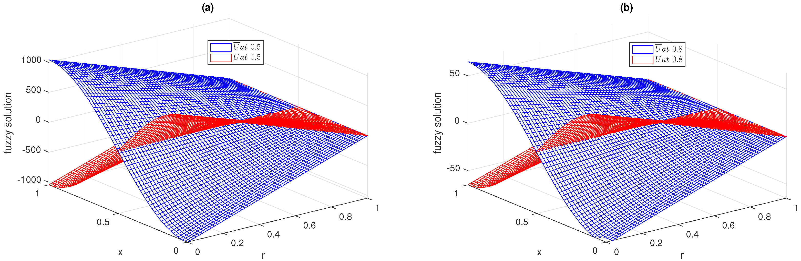
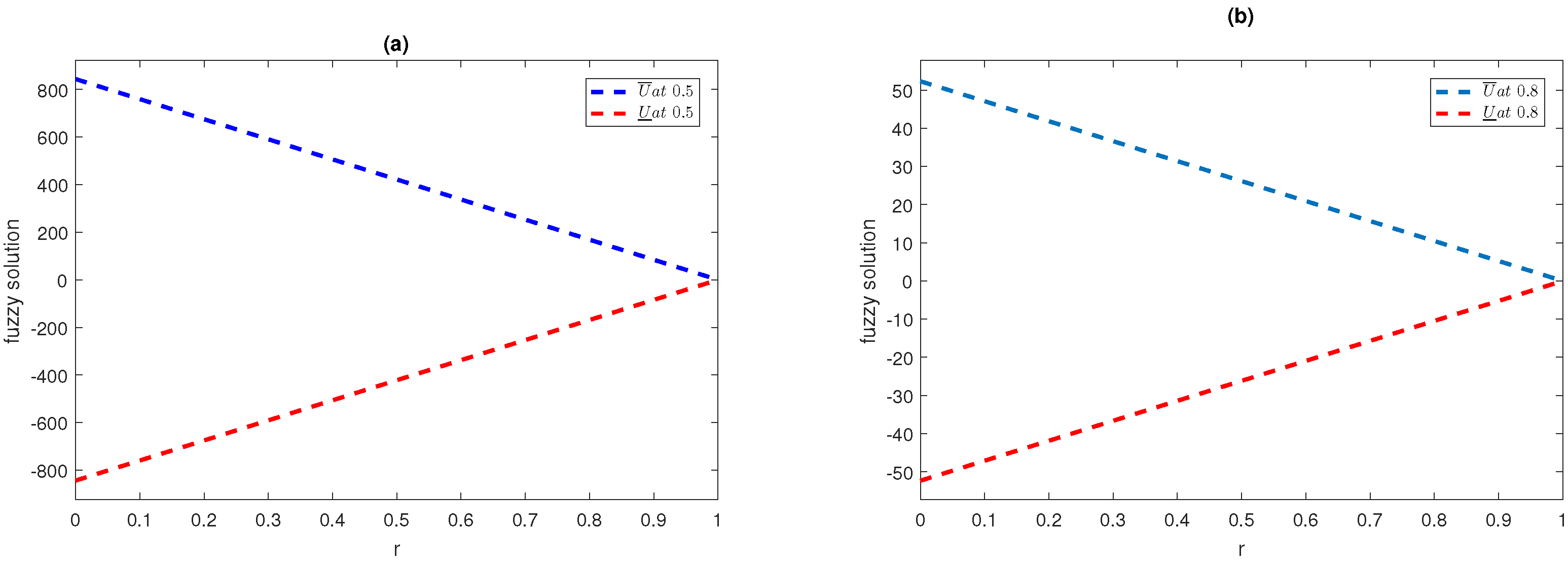
4. Examples

Now, in this part, we provide some illustrations of 2D fuzzy arbitrary-order heat equations with external source terms by applying the aforementioned method for obtaining the approximate results.

Example 1.

The first example is of a fuzzy heat equation of fractional order having the external source term $\mathcal{F}(\tau ,x_2,x_1)=(x_2+x_1+1)$ along with a fuzzy initial condition as in [12,13,14], as follows: -5.0cm0cm

$$\begin{array}{ccc}\hfill {\mathcal{D}}_{\tau }^{\theta }\tilde{\mathrm{U}}(\tau ,x_2,x_1)& =& {\mathcal{D}}_{x_1}^2\tilde{\mathrm{U}}(\tau ,x_2,x_1)+{\mathcal{D}}_{x_2}^2\tilde{\mathrm{U}}(\tau ,x_2,x_1)+\tilde{k}\left(r\right)(x_2+x_1+1),0<\theta \le 1,0<x_2,x_1<1,\hfill \\ \hfill \tilde{\mathrm{U}}(x_2,x_1,0)& =& \tilde{k}\left(r\right)exp(-(x_2+x_1)).\hfill \end{array}$$

(13)

Using the scheme of Equation (11), we obtain

$$\begin{array}{ccc}\hfill {\underline{\mathrm{U}}}_0(\tau ,x_2,x_1)& =& \underline{k}\left(r\right)exp[-(x_2+x_1)]+\underline{k}\left(r\right)(x_2+x_1+1)\left[1+\theta \tau -\theta \right],\hfill \\ \hfill {\overline{\mathrm{U}}}_0(\tau ,x_2,x_1)& =& exp[-(x_2+x_1)]\overline{k}\left(r\right)+(x_2+x_1+1)\overline{k}\left(r\right)\left[1+\theta \tau -\theta \right],\hfill \\ \hfill {\underline{\mathrm{U}}}_1(\tau ,x_2,x_1)& =& 2\underline{k}\left(r\right)exp[-(x_2+x_1)]\left[1+\theta \tau -\theta \right],\hfill \\ \hfill {\overline{\mathrm{U}}}_1(\tau ,x_2,x_1)& =& 2\overline{k}\left(r\right)exp[-(x_2+x_1)]\left[1+\theta \tau -\theta \right],\hfill \\ \hfill {\underline{\mathrm{U}}}_2(\tau ,x_2,x_1)& =& 4\underline{k}\left(r\right)exp[-(x_2+x_1)]\left[(1-\theta )2\theta \tau +{(1-\theta )}^2+\frac{{\theta }^2{\tau }^2}{2}\right],\hfill \\ \hfill {\overline{\mathrm{U}}}_2(\tau ,x_2,x_1)& =& 4\overline{k}\left(r\right)exp[-(x_2+x_1)]\left[(1-\theta )2\theta \tau +{(1-\theta )}^2+\frac{{\theta }^2{\tau }^2}{2}\right],\hfill \\ \hfill {\underline{\mathrm{U}}}_3(\tau ,x_2,x_1)& =& 8\underline{k}\left(r\right)exp[-(x_2+x_1)]\left[{(1-\theta )}^{2}3\theta \tau +{(1-\theta )}^3+\frac{3{\theta }^2(1-\theta ){\tau }^2}{2}+\frac{{\theta }^3{\tau }^3}{3!}\right],\hfill \\ \hfill {\overline{\mathrm{U}}}_3(\tau ,x_2,x_1)& =& 8\overline{k}\left(r\right)exp[-(x_2+x_1)]\left[{(1-\theta )}^3+3\theta {(1-\theta )}^2\tau +\frac{3{\theta }^2(1-\theta ){\tau }^2}{2}+\frac{{\theta }^3{\tau }^3}{3!}\right],\hfill \\ \hfill {\underline{\mathrm{U}}}_4(\tau ,x_2,x_1)& =& 16\underline{k}\left(r\right)exp[-(x_2+x_1)][{(1-\theta )}^4+4\theta {(1-\theta )}^3\tau +\frac{4{\theta }^2{(1-\theta )}^2{\tau }^2}{2}+\hfill \\ & & \frac{4{\theta }^3(1-\theta ){\tau }^3}{3!}+\frac{{\theta }^4{\tau }^4}{4!}],\hfill \\ \hfill {\overline{\mathrm{U}}}_4(\tau ,x_2,x_1)& =& 16\overline{k}\left(r\right)exp[-(x_2+x_1)][{(1-\theta )}^4+4\theta {(1-\theta )}^3\tau +\frac{4{\theta }^2{(1-\theta )}^2{\tau }^2}{2}+\hfill \\ & & \frac{4{\theta }^3(1-\theta ){\tau }^3}{3!}+\frac{{\theta }^4{\tau }^4}{4!}]\hfill \end{array}$$

(14)

In a similar fashion, we can obtain the higher terms. The series solution is obtained using Equation (12); therefore, we write

$$\tilde{U}(\tau ,x_2,x_1)={\tilde{U}}_0(\tau ,x_2,x_1)+{\tilde{U}}_1(\tau ,x_2,x_1)+{\tilde{U}}_2(\tau ,x_2,x_1)\dots ,$$

while, in upper and lower portion form, it is

$$\begin{array}{c}\hfill \underline{U}(\tau ,x_2,x_1)={\underline{U}}_0(\tau ,x_2,x_1)+{\underline{U}}_1(\tau ,x_2,x_1)+{\underline{U}}_2(\tau ,x_2,x_1)\dots ,\\ \hfill \overline{U}(\tau ,x_2,x_1)={\overline{U}}_0(\tau ,x_2,x_1)+{\overline{U}}_1(\tau ,x_2,x_1)+{\overline{U}}_2(\tau ,x_2,x_1)\dots .\end{array}$$

Figure 1 is the representation of a 3D plot, showing the upper and lower branches of a fuzzy solution for a fractional-order heat equation at $x_1=0.8,x_2=0.5$, and at two different fractional orders of θ. Figure 2 shows the dynamical behavior of the upper and lower branches of the fuzzy solution for the fractional-order heat equation of Example 1 at $x_1=0.8,x_2=0.5,and\tau =0.5$ and at various fractional orders of θ and $r\in [0,1]$. The curve in both the 2D and 3D cases for the lower and upper portions begins from zero and continues to positive and negative values. This is also because $\tilde{k}\left(r\right)=[\overline{k}\left(r\right),\underline{k}\left(r\right)]=[1-r,r-1],$ and $\overline{k}\left(r\right)=1-r,r\in [0,1]$ provides the upward portion or positive fuzzy solution, while $\underline{k}\left(r\right)=[r-1],r\in [0,1]$ provides the lower portion or negative fuzzy solution.

Example 2.

Take another illustration of the fuzzy fractional heat equation having the external source term $\mathcal{F}(\tau ,x_2,x_1)={\tau }^2+x_2+x_1$ with an initial approximation as in [12,13,14] as follows:

$$\begin{array}{ccc}\hfill {}^{CF}{\mathcal{D}}_{\tau }^{\theta }\tilde{\mathrm{U}}(\tau ,x_2,x_1)& =& {\mathcal{D}}_{x_1}^2\tilde{\mathrm{U}}(\tau ,x_2,x_1)+{\mathcal{D}}_{x_2}^2\tilde{\mathrm{U}}(\tau ,x_2,x_1)+{\tau }^2+x_2+x_1,0<\theta \le 1,\hfill \\ \hfill \tilde{\mathrm{U}}(0,x_2,x_1)& =& \tilde{k}\left(r\right)sin\left((x_1+x_2)\pi \right),0<x_2,x_1<1,\hfill \end{array}$$

(15)

$\tilde{k}\left(r\right)=[\overline{k}\left(r\right),\underline{k}\left(r\right)]=[1-r,r-1].$ Upon the application of the Laplace transform of the Caputo–Fabrizio derivative, one may obtain

$$\begin{array}{ccc}\hfill {\underline{\mathrm{U}}}_0(\tau ,x_2,x_1)& =& sin\left((x_1+x_2)\pi \right)\underline{k}\left(r\right)+(x_2+x_1)[1+\theta \tau -\theta ]+2\left[\frac{{\tau }^2}{2}+\frac{\theta {\tau }^3}{3!}-\frac{\theta {\tau }^2}{2}\right],\hfill \\ \hfill {\overline{\mathrm{U}}}_0(\tau ,x_2,x_1)& =& sin\left(\pi (x_2+x_1)\right)\overline{k}\left(r\right)+(x_2+x_1[1+\theta \tau -\theta ]+2\left[\frac{{\tau }^2}{2}+\frac{\theta {\tau }^3}{3!}-\frac{\theta {\tau }^2}{2}\right],\hfill \\ \hfill {\underline{\mathrm{U}}}_1(\tau ,x_2,x_1)& =& [-2{\pi }^{2}sin\left((x_1+x_2)\pi \right)\underline{k}\left(r\right)(1+\theta \tau -\theta )],\hfill \\ \hfill {\overline{\mathrm{U}}}_1(\tau ,x_2,x_1)& =& [-2{\pi }^{2}sin\left((x_1+x_2)\pi \right)\overline{k}\left(r\right)(1+\theta \tau -\theta )],\hfill \\ \hfill {\underline{\mathrm{U}}}_2(\tau ,x_2,x_1)& =& 4{\pi }^{4}sin\left((x_1+x_2)\pi \right)\underline{k}\left(r\right)\left[(1-\theta )2\theta \tau +{(1-\theta )}^2+\frac{{\theta }^2{\tau }^2}{2}\right],\hfill \\ \hfill {\overline{\mathrm{U}}}_2(\tau ,x_2,x_1)& =& 4{\pi }^{4}sin\left((x_2+x_1)\pi \right)\overline{k}\left(r\right)\left[(1-\theta )2\theta \tau +{(1-\theta )}^2+\frac{{\theta }^2{\tau }^2}{2}\right],\hfill \end{array}$$

$$\begin{array}{ccc}\hfill {\underline{\mathrm{U}}}_3(\tau ,x_2,x_1)& =& -8{\pi }^{6}sin\left((x_1+x_2)\pi \right)\underline{k}\left(r\right)\left[{(1-\theta )}^{2}3\theta \tau +{(1-\theta )}^3+\frac{3{\theta }^2(1-\theta ){\tau }^2}{2}+\frac{{\theta }^3{\tau }^3}{3!}\right],\hfill \\ \hfill {\overline{\mathrm{U}}}_3(\tau ,x_2,x_1)& =& -8{\pi }^{6}sin\left((x_1+x_2)\pi \right)\overline{k}\left(r\right)\left[{(1-\theta )}^{2}3\theta \tau +{(1-\theta )}^3+\frac{3{\theta }^2(1-\theta ){\tau }^2}{2}+\frac{{\theta }^3{\tau }^3}{3!}\right],\hfill \\ \hfill {\underline{\mathrm{U}}}_4(\tau ,x_2,x_1)& =& 16{\pi }^{8}sin\left((x_1+x_2)\pi \right)\underline{k}\left(r\right)[{(1-\theta )}^4+4\theta {(1-\theta )}^3\tau +\frac{4{\theta }^2{(1-\theta )}^2{\tau }^2}{2}+\hfill \\ & & \frac{4{\theta }^3(1-\theta ){\tau }^3}{3!}+\frac{{\theta }^4{\tau }^4}{4!}],\hfill \\ \hfill {\overline{\mathrm{U}}}_4(\tau ,x_2,x_1)& =& 16\left(r\right){\pi }^{8}sin\left((x_1+x_2)\pi \right)\overline{k}\left(r\right)[{(1-\theta )}^4+4\theta {(1-\theta )}^3\tau +\frac{4{\theta }^2{(1-\theta )}^2{\tau }^2}{2}+\hfill \\ & & \frac{4{\theta }^3(1-\theta ){\tau }^3}{3!}+\frac{{\theta }^4{\tau }^4}{4!}],\hfill \end{array}$$

(16)

From (12), we can write $\tilde{U}(\tau ,x_2,x_1)={\tilde{U}}_0(\tau ,x_2,x_1)+{\tilde{U}}_1(\tau ,x_2,x_1)+{\tilde{U}}_2(\tau ,x_2,x_1)\dots$ such that

$$\begin{array}{c}\hfill \underline{U}(\tau ,x_2,x_1)={\underline{U}}_0(\tau ,x_2,x_1)+{\underline{U}}_1(\tau ,x_2,x_1)+{\underline{U}}_2(\tau ,x_2,x_1)\dots \\ \hfill \overline{U}(\tau ,x_2,x_1)={\overline{U}}_0(\tau ,x_2,x_1)+{\overline{U}}_1(\tau ,x_2,x_1)+{\overline{U}}_2(\tau ,x_2,x_1)\dots \end{array}$$

Figure 3 is the 3D plot showing the upper and lower portions of the fuzzy solution for the fractional-order fuzzy heat equation of Example 2 at $x_1=0.8,x_2=0.5$, and at various fractional orders of θ. Figure 4 shows the behavior of the upper and lower portions of the fuzzy solution in two-dimensional format for the fractional-order heat equation of Example 2 at $x_1=0.8,x_2=0.5,\tau =0.5$, and at various fractional orders of θ and $r\in [0,1]$. Like for the first example, the curve in both the 2D and 3D cases for the lower and upper portions begins from zero and continues to positive and negative values. This is also due to $\tilde{k}\left(r\right)=[\overline{k}\left(r\right),\underline{k}\left(r\right)]=[1-r,r-1],$ $\overline{k}\left(r\right)=1-r,r\in [0,1]$ providing the upward portion or positive fuzzy solution, while $\underline{k}\left(r\right)=[r-1],r\in [0,1]$ provides the lower portion or negative fuzzy solution.

Example 3.

Let us consider the last example of a non-integer-order heat equation having uncertainty in the initial condition along with the source term $\mathcal{F}(\tau ,x_2,x_1)={\tau }^4+x_2+x_1$ like in [12,13,14] as follows:

$$\begin{array}{ccc}\hfill {}^{CF}{\mathcal{D}}_{\tau }^{\theta }\tilde{\mathrm{U}}(\tau ,x_2,x_1)& =& \frac{1}{2}(x_2+x_1^2)[{\mathcal{D}}_{x_1}^2\tilde{\mathrm{U}}(\tau ,x_2,x_1)+{\mathcal{D}}_{x_2}^2]\tilde{\mathrm{U}}(\tau ,x_2,x_1)++{\tau }^4+x_2+x_1,0<\theta \le 1,\hfill \\ \hfill \tilde{\mathrm{U}}(0,x_2,x_1)=& =& {(x_2+x_1)}^2\tilde{K}(r),0<x_2,x_1<1.\hfill \end{array}$$

(17)

Using the scheme of Laplace transform and by the decomposition of $\tilde{\mathrm{U}}(\tau ,x_2,x_1)$ into small terms, we obtain a hierarchy of terms as follows:

$$\begin{array}{ccc}\hfill {\underline{\mathrm{U}}}_0(\tau ,x_2,x_1)& =& {(x_2+x_1)}^2\underline{k}\left(r\right)+(x_2+x_1)[1+\theta \tau -\theta ]+4!\left[\frac{{\tau }^4}{4!}+\frac{\theta {\tau }^5}{5!}-\frac{\theta {\tau }^4}{4!}\right],\hfill \\ \hfill {\overline{\mathrm{U}}}_0(\tau ,x_2,x_1)& =& {(x_2+x_1)}^2\overline{k}\left(r\right)+(x_2+x_1[1+\theta \tau -\theta ]+4!\left[\frac{{\tau }^4}{4!}+\frac{\theta {\tau }^5}{5!}-\frac{\theta {\tau }^4}{4!}\right],\hfill \\ \hfill {\underline{\mathrm{U}}}_1(\tau ,x_2,x_1)& =& [2{(x_2+x_1)}^2[1+\theta \tau -\theta ]\underline{k}\left(r\right),\hfill \\ \hfill {\overline{\mathrm{U}}}_1(\tau ,x_2,x_1)& =& [2{(x_2+x_1)}^2[1+\theta \tau -\theta ]\overline{k}\left(r\right),\hfill \\ \hfill {\underline{\mathrm{U}}}_2(\tau ,x_2,x_1)& =& 4{(x_2+x_1)}^2\left[(1-\theta )2\theta \tau +{(1-\theta )}^2+\frac{{\theta }^2{\tau }^2}{2}\right]\underline{k}\left(r\right),\hfill \\ \hfill {\overline{\mathrm{U}}}_2(\tau ,x_2,x_1)& =& 4{(x_2+x_1)}^2\left[(1-\theta )2\theta \tau +{(1-\theta )}^2+\frac{{\theta }^2{\tau }^2}{2}\right]\overline{k}\left(r\right),\hfill \\ \hfill {\underline{\mathrm{U}}}_3(\tau ,x_2,x_1)& =& 8{(x_2+x_1)}^2\left[{(1-\theta )}^{2}3\theta \tau +{(1-\theta )}^3+\frac{3{\theta }^2(1-\theta ){\tau }^2}{2}+\frac{{\theta }^3{\tau }^3}{3!}\right]\underline{k}\left(r\right),\hfill \\ \hfill {\overline{\mathrm{U}}}_3(\tau ,x_2,x_1)& =& 8{(x_2+x_1)}^2\left[{(1-\theta )}^{2}3\theta \tau +{(1-\theta )}^3+\frac{3{\theta }^2(1-\theta ){\tau }^2}{2}+\frac{{\theta }^3{\tau }^3}{3!}\right]\overline{k}\left(r\right),\hfill \end{array}$$

$$\begin{array}{ccc}\hfill {\underline{\mathrm{U}}}_4(\tau ,x_2,x_1)& =& 16{(x_2+x_1)}^2[{(1-\theta )}^4+4\theta {(1-\theta )}^3\tau +\frac{4{\theta }^2{(1-\theta )}^2{\tau }^2}{2}+\hfill \\ & & \frac{4{\theta }^3(1-\theta ){\tau }^3}{3!}+\frac{{\theta }^4{\tau }^4}{4!}]\underline{k}\left(r\right),\hfill \\ \hfill {\overline{\mathrm{U}}}_4(\tau ,x_2,x_1)& =& 16{(x_2+x_1)}^2[{(1-\theta )}^4+4\theta {(1-\theta )}^3\tau +\frac{4{\theta }^2{(1-\theta )}^2{\tau }^2}{2}+\hfill \\ & & \frac{4{\theta }^3(1-\theta ){\tau }^3}{3!}+\frac{{\theta }^4{\tau }^4}{4!}]\overline{k}\left(r\right).\hfill \end{array}$$

(18)

Now, we can write all the decomposed terms into sum form as

$$\tilde{U}(\tau ,x_2,x_1)={\tilde{U}}_0(\tau ,x_2,x_1)+{\tilde{U}}_1(\tau ,x_2,x_1)+{\tilde{U}}_2(\tau ,x_2,x_1)\dots ,$$

such that

$$\begin{array}{c}\hfill \underline{U}(\tau ,x_2,x_1)={\underline{U}}_0(\tau ,x_2,x_1)+{\underline{U}}_1(\tau ,x_2,x_1)+{\underline{U}}_2(\tau ,x_2,x_1)\dots ,\\ \hfill \overline{U}(\tau ,x_2,x_1)={\overline{U}}_0(\tau ,x_2,x_1)+{\overline{U}}_1(\tau ,x_2,x_1)+{\overline{U}}_2(\tau ,x_2,x_1)\dots .\end{array}$$

In Figure 5, we have drawn a 3D plot showing the upper and lower regions of the fuzzy solution for the fractional-order fuzzy heat equation at $x_1=0.8,x_2=0.5$, and at different fractional orders of θ. Figure 6 shows the fuzzy solution of the upper and lower portions for the fractional-order heat equation at $x_1=0.8,x_2=0.5,\tau =0.5$, and at different fractional orders of θ and $r\in [0,1]$. The curve in both the 2D and 3D cases for the lower and upper portions begin from zero and continue to positive and negative values. This is due to the fuzzy number $\tilde{k}\left(r\right)=[\overline{k}\left(r\right),\underline{k}\left(r\right)]=[1-r,r-1],$ $\overline{k}\left(r\right)=1-r,r\in [0,1]$, providing the above portion or positive fuzzy solution, while $\underline{k}\left(r\right)=[r-1],r\in [0,1]$, provides the below portion or negative fuzzy solution.

5. Conclusions and Discussion

Finally, we conclude that a successful scheme for the computation of semi-analytical or approximate solutions has been used for two-dimensional fuzzy fractional-order diffusion or heat partial differential equations having diffusion terms as external terms. The techniques of Laplace Adomian decomposition (LADM) were applied for the analysis of a semi-analytical solution in the form of a series solution and may be used for different fractional-order problems. We also verified our general techniques of solution using three specific illustrations. All of the three examples were analyzed using the said techniques by taking account of the uncertainty in the initial values by multiplying the fuzzy number at two different fractional orders. The obtained results for all the three examples were simulated with two different formats of 2D and 3D graphs. The achieved results were also obtained in the form of uncertainty, having upper branches and lower branches of fuzzy solutions. We may also take different values of fractional orders to check and compare them with the integer order. By increasing the order of $\theta$, we can converge to the value of integer order 1. For the future, the implementation of this scheme may be applied to different partial differential equations for series-type solutions, for both integer and non-integer orders in fuzzy form. Furthermore, the adopted techniques can be used as a robust tool to study fractional-order non-linear and linear dynamical systems.

References

- Podlubny, I. Fractional Differential Equations, Mathematics in Science and Engineering; Academic Press: New York, NY, USA, 1999. [Google Scholar]
- Lakshmikantham, V.; Leela, S.; Vasundhara, J. Theory of Fractional Dynamic Systems; Cambridge Academic Publishers: Cambridge, UK, 2009. [Google Scholar]
- Hilfer, R. Applications of Fractional Calculus in Physics; World Scientific: Singapore, 2000. [Google Scholar]
- Rahman, N.A.A.; Ahmad, M.Z. Solving fuzzy fractional differential equations using fuzzy Sumudu transform. J. Nonlinear Sci. Appl. 2017, 10, 2620–2632. [Google Scholar] [CrossRef]
- Rossikhin, Y.A.; Shitikova, M.V. Applications of fractional calculus to dynamic problems of linear and nonlinear hereditary mechanics of solids. Appl. Mech. Rev. 1997, 50, 15–67. [Google Scholar] [CrossRef]
- Zadeh, L.A. Fuzzy sets. Inf. Control 1965, 8, 338–353. [Google Scholar] [CrossRef] [Green Version]
- Chang, S.S.; Zadeh, L.A. On Fuzzy Mapping and Control: In Fuzzy Sets, Fuzzy Logic, and Fuzzy Systems: Selected Papers by Lotfi A Zadeh; World Scientific: Singapore, 1996. [Google Scholar]
- Prade, H.; Dubois, D. Towards fuzzy differential calculus. Fuzzy Sets Syst. 1982, 8, 225–233. [Google Scholar]
- Goetschel, J.R.; Voxman, W. Elementary fuzzy calculus. Fuzzy Sets Syst. 1986, 18, 31–43. [Google Scholar] [CrossRef]
- Kaleva, O. Fuzzy differential equations. Fuzzy Sets Syst. 1987, 24, 301–317. [Google Scholar] [CrossRef]
- Wang, L.; Wang, L. A Course in Fuzzy Systems and Control; Prentice Hall PTR: Upper Saddle River, NJ, USA, 1997. [Google Scholar]
- Ahmad, M.Z.; Hasan, M.K.; Abbasbandy, S. Solving fuzzy fractional differential equations using Zadehs extension principle. Sci. World J. 2013, 2013, 454969. [Google Scholar] [CrossRef] [Green Version]
- Pirzada, U.M.; Vakaskar, D.C. Solution of fuzzy heat equations using Adomian Decomposition. Int. J. Adv. Appl. Math. Mech. 2015, 3, 87–91. [Google Scholar]
- Chakraverty, S.; Tapaswini, S.; Behera, D. Fuzzy Fractional Heat Equations; John Wiley & Sons, Inc.: Hoboken, NJ, USA, 2016. [Google Scholar]
- Yavuz, M.; Özdemir, N. European vanilla option pricing model of fractional order without singular kernel. Fractal Fract. 2018, 2, 3. [Google Scholar] [CrossRef] [Green Version]
- Veeresha, P. A numerical approach to the coupled atmospheric ocean Model using a fractional Operator. Math. Model. Numer. Simul. Appl. (MMNSA) 2021, 1, 1–10. [Google Scholar]
- Arfan, M.; Shah, K.; Abdeljawad, T.; Hammouch, Z. An efficient tool for solving two-dimensional fuzzy fractional-ordered heat equation. Numer. Methods Partial. Differ. Equ. 2020, 37, 1407–1418. [Google Scholar] [CrossRef]
- Hammouch, Z.; Yavuz, M.; Özdemir, N. Numerical solutions and synchronization of a variable-order fractional chaotic system. Math. Model. Numer. Simul. Appl. (MMNSA) 2021, 1, 11–23. [Google Scholar]
- Akgül, E.K.; Akgül, A.; Yavuz, M. New illustrative applications of integral transforms to financial models with different fractional derivatives. Chaos Solitons Fractals 2021, 146, 110877. [Google Scholar] [CrossRef]
- Shah, K.; Seadawy, A.R.; Arfan, M. Evaluation of one dimensional fuzzy fractional partial differential equations. Alex. Eng. J. 2020, 59, 3347–3353. [Google Scholar]
- Ullah, I.; Ahmad, S.; Rahman, M.U.; Arfan, M. Investigation of fractional order Tuberculosis (TB) model via caputo derivative. Chaos Solitons Fractals 2021, 142, 110479. [Google Scholar] [CrossRef]
- Shen, W.Y.; Chu, Y.M.; ur Rahman, M.; Mahariq, I.; Zeb, A. Mathematical Analysis of HBV and HCV Co-infection Model Under Nonsingular Fractional Order Derivative. Results Phys. 2021, 28, 104582. [Google Scholar] [CrossRef]
- Nazir, G.; Zeb, A.; Shah, K.; Saeed, T.; Khan, R.A.; Khan, S.I.U. Study of COVID-19 Mathematical Model of Fractional Order Via Modified Euler Method. AEJ Alex. Eng. J. 2021, 60, 5287–5296. [Google Scholar] [CrossRef]
- Atangana, A.; Koca, I. Chaos in a simple nonlinear system with Atangana-Baleanu derivatives with fractional order. Chas Solitons Fractals 2016, 89, 447–454. [Google Scholar] [CrossRef]
- Tofigh, A.; Ghanbari, B. On the fuzzy fractional differential equation with interval Atangana-Baleanu fractional derivative approach. Chaos Solitons Fractals 2020, 130, 109397. [Google Scholar]
- Abdon, A.; Gómez-Aguilar, J.F. Numerical approximation of Riemann-Liouville definition of fractional derivative: From Riemann-Liouville to Atangana-Baleanu. Numer. Methods Partial. Differ. Equ. 2018, 34, 1502–1523. [Google Scholar]
- Gómez-Aguilar, J.F.; Atangana, A.; Morales-Delgado, V.F. Electrical circuits RC, LC, and RL described by Atangana-Baleanu fractional derivatives. Int. J. Circ. Theory Appl. 2017, 45, 1514–1533. [Google Scholar] [CrossRef]
- Zhang, Y. Initial boundary value problem for fractal heat equation in the semi-infinite region by Yang-Laplace transform. Therm. Sci. 2014, 18, 677–681. [Google Scholar] [CrossRef]
- Atangana, A. Mathematical model of survival of fractional calculus, critics and their impact: How singular is our world? Adv. Differ. Equ. 2021, 2021, 403. [Google Scholar] [CrossRef]
- Avci, D.; Yavuz, M.; Özdemir, N. Fundamental solutions to the Cauchy and Dirichlet problems for a heat conduction equation equipped with the Caputo-Fabrizio differentiation. In Heat Conduction: Methods, Applications and Research; Nova Science Publishers: Hauppauge, NY, USA, 2019; pp. 95–107. [Google Scholar]
- Evirgen, F.; Yavuz, M. An alternative approach for nonlinear optimization problem with Caputo-Fabrizio derivative. In ITM Web of Conferences; EDP Sciences: Les Ulis, France, 2018; Volume 22, p. 01009. [Google Scholar]
- Yavuz, M.; Özdemir, N. Numerical inverse Laplace homotopy technique for fractional heat equations. Therm. Sci. 2018, 22, 185–194. [Google Scholar] [CrossRef]
- Lin, J.; Feng, W.; Reutskiy, S.; Xu, H.; He, Y. A semi-analytical method for solving a class of time fractional partial differential equations with variable coefficients. Appl. Math. Lett. 2021, 112, 106712. [Google Scholar] [CrossRef]
- Lin, J. Homogenization function method for 2D and 3D inverse source problems of nonlinear time-fractional wave equation. Eng. Comput. 2021. [Google Scholar] [CrossRef]
- Eltayeb, H.; Kiliçman, A. A note on solutions of wave, Laplace’s and heat equations with convolution terms by using a double Laplace transform. Appl. Math. Lett. 2008, 21, 1324–1329. [Google Scholar] [CrossRef] [Green Version]
- Yu, Z. Povstenko, Fractional heat conduction equation and associated thermal stress. J. Therm. Stress. 2004, 28, 83–102. [Google Scholar]
- Allahviranloo, T.; Taheri, N. An analytic approximation to the solution of fuzzy heat equation by Adomian decomposition method. Int. J. Contemp. Math. Sci. 2009, 4, 105–114. [Google Scholar]
- Richard, H. Elementary Applied Partial Differential Equations; Prentice Hall: Englewood Cliffs, NJ, USA, 1983. [Google Scholar]
- Rizzo, F.J.; Shippy, D.J. A method of solution for certain problems of transient heat conduction. AIAA J. 1970, 8, 2004–2009. [Google Scholar] [CrossRef]
- Khan, T.; Shah, K.; Khan, R.A.; Khan, A. Solution of fractional order heat equation via triple Laplace transform in 2 dimensions. Math. Methods Appl. Sci. 2018, 41, 818–825. [Google Scholar] [CrossRef]
- Baleanu, D.; Mousalou, A.; Rezapour, S. A new method for investigating approximate solutions of some fractional integro-differential equations involving the Caputo-Fabrizio derivative. Adv. Differ. Equn 2017, 2017, 51. [Google Scholar] [CrossRef] [Green Version]
- Shah, K.; Khalil, H.; Khan, R.A. Analytical solutions of fractional order diffusion equations by natural transform method. Iran. J. Sci. Technol. Trans. A Sci. 2018, 42, 1479–1490. [Google Scholar] [CrossRef]
Publisher’s Note: MDPI stays neutral with regard to jurisdictional claims in published maps and institutional affiliations. |
© 2021 by the authors. Licensee MDPI, Basel, Switzerland. This article is an open access article distributed under the terms and conditions of the Creative Commons Attribution (CC BY) license (https://creativecommons.org/licenses/by/4.0/).
Share and Cite
Sitthiwirattham, T.; Arfan, M.; Shah, K.; Zeb, A.; Djilali, S.; Chasreechai, S. Semi-Analytical Solutions for Fuzzy Caputo–Fabrizio Fractional-Order Two-Dimensional Heat Equation. Fractal Fract. 2021, 5, 139. https://doi.org/10.3390/fractalfract5040139
Sitthiwirattham T, Arfan M, Shah K, Zeb A, Djilali S, Chasreechai S. Semi-Analytical Solutions for Fuzzy Caputo–Fabrizio Fractional-Order Two-Dimensional Heat Equation. Fractal and Fractional. 2021; 5(4):139. https://doi.org/10.3390/fractalfract5040139
Chicago/Turabian StyleSitthiwirattham, Thanin, Muhammad Arfan, Kamal Shah, Anwar Zeb, Salih Djilali, and Saowaluck Chasreechai. 2021. "Semi-Analytical Solutions for Fuzzy Caputo–Fabrizio Fractional-Order Two-Dimensional Heat Equation" Fractal and Fractional 5, no. 4: 139. https://doi.org/10.3390/fractalfract5040139
APA StyleSitthiwirattham, T., Arfan, M., Shah, K., Zeb, A., Djilali, S., & Chasreechai, S. (2021). Semi-Analytical Solutions for Fuzzy Caputo–Fabrizio Fractional-Order Two-Dimensional Heat Equation. Fractal and Fractional, 5(4), 139. https://doi.org/10.3390/fractalfract5040139