
Effect of Magnetic Field with Parabolic Motion on Fractional Second Grade Fluid


Abstract
:1. Introduction
2. Mathematical Modeling
3. Solution for Caputo Fractional Operator
3.1. Temperature Field
3.2. Concentration Field
3.3. Velocity Field
4. Solution for Caputo–Fabrizio Fractional Operator
4.1. Temperature Field
4.2. Concentration Field
4.3. Velocity Field
5. Solution for Atangana–Baleanu Fractional Operator
5.1. Temperature Field
5.2. Concentration Field
5.3. Velocity Field
6. Results and Discussion

7. Conclusions
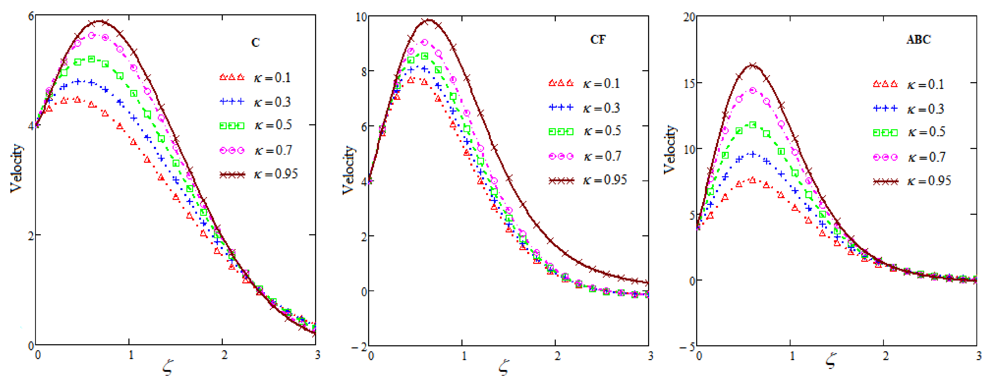
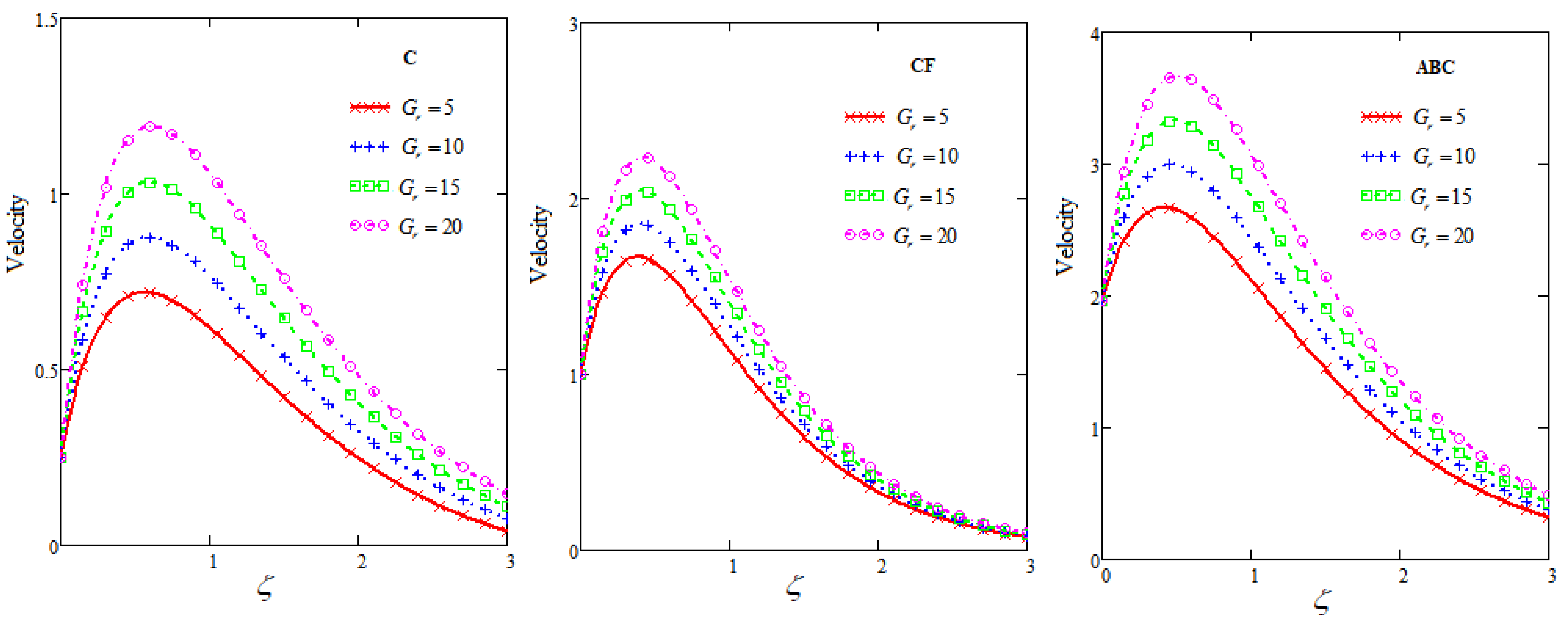
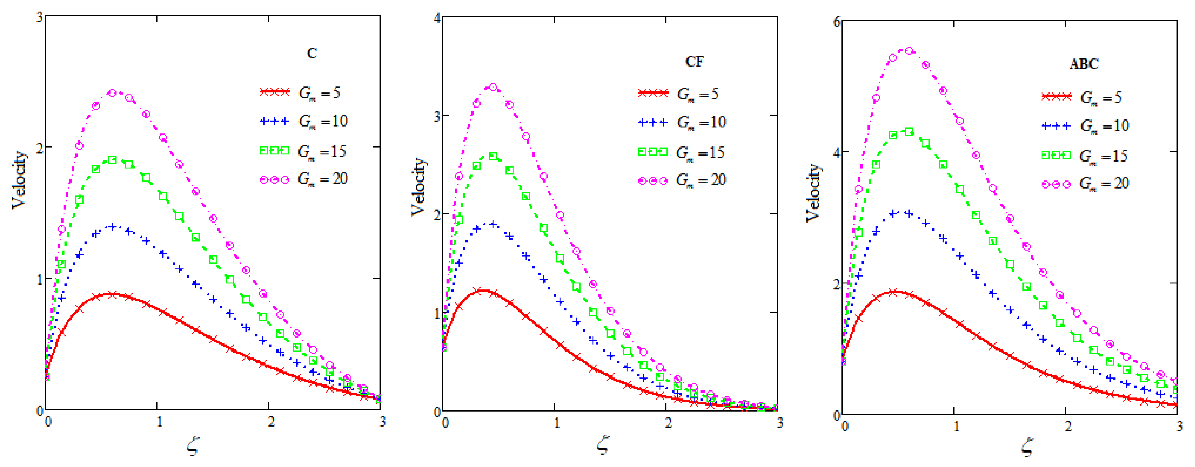
- Velocity curves are increasing for greater values of , and .
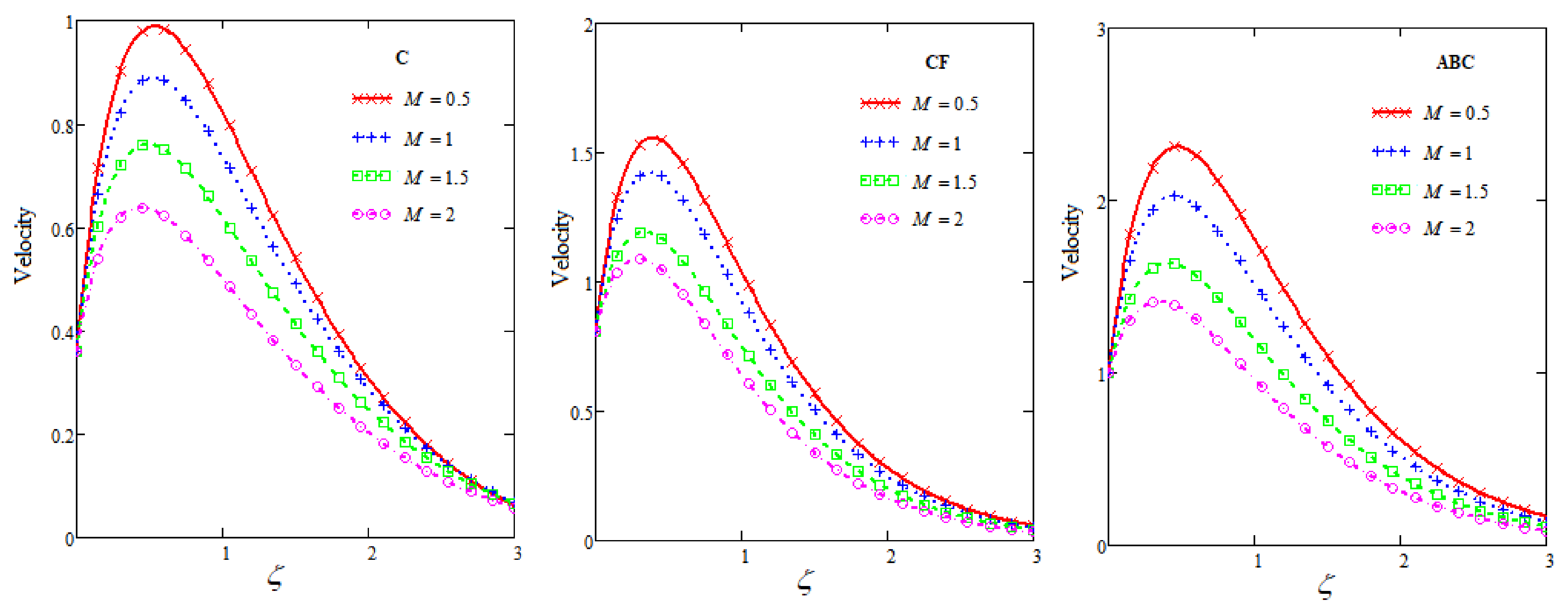
- Fluid flow descends for and M.
- Velocity and concentration curves show a decreasing behavior under the influence of .
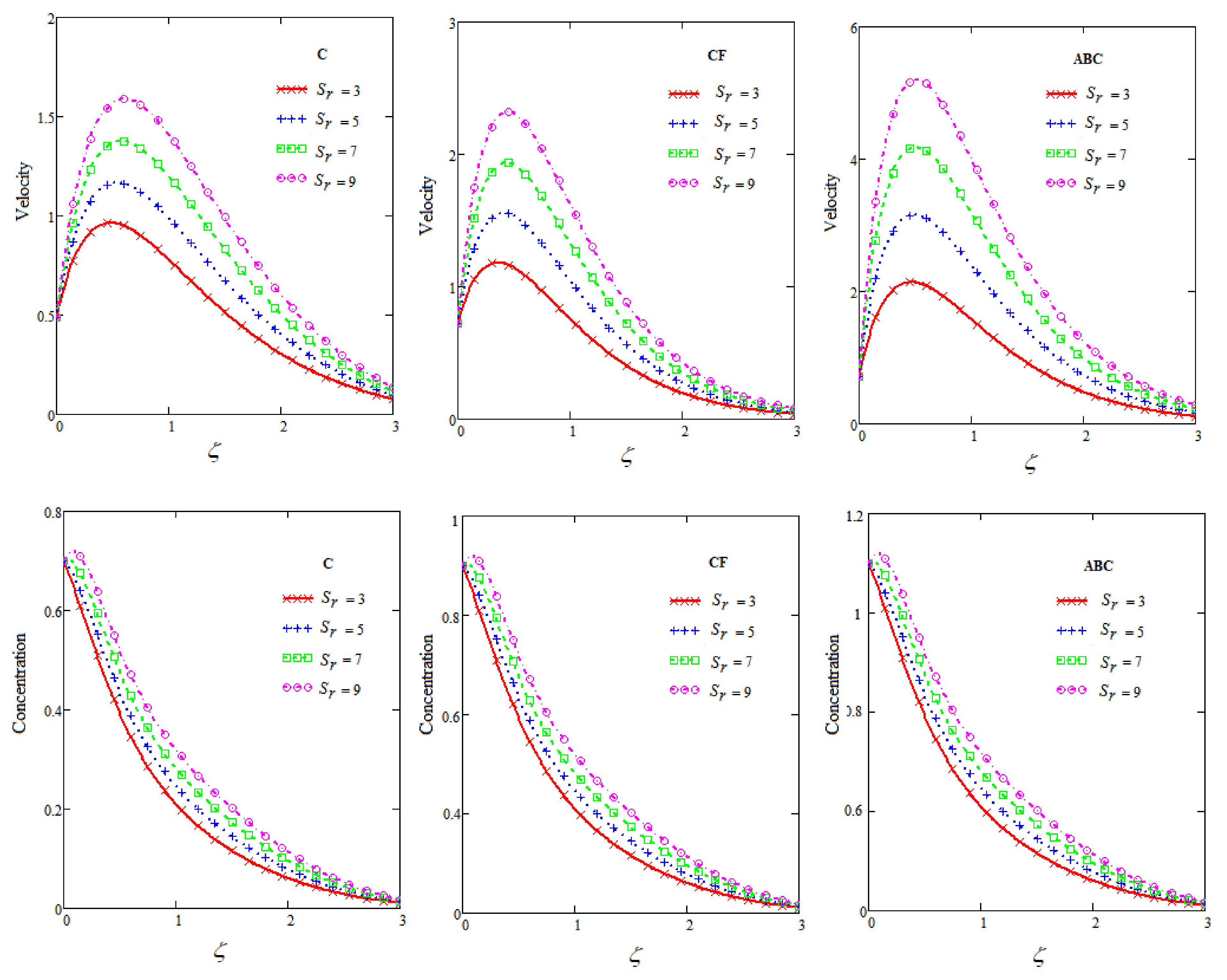
- Fluid velocity accelerates under the impact of and R.
- Heat and mass profiles for and R are show an increasing behavior.
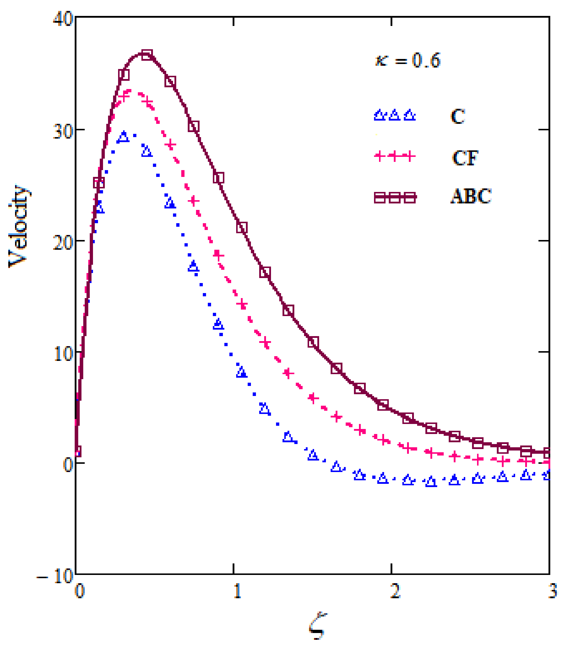
- Curves show prominent behavior for ABC among C, CF and ABC.
Author Contributions
Funding
Institutional Review Board Statement
Informed Consent Statement
Data Availability Statement
Acknowledgments
Conflicts of Interest
Nomenclature
| Symbol | Quantity |
| w | Velocity of the fluid |
| Temperature of the fluid | |
| C | Concentration of the fluid |
| g | Acceleration due to gravity |
| k | Thermal conductivity of the fluid |
| Permeability parameter | |
| Parameter of chemical reaction | |
| M | Parameter of magnetic field |
| Coefficient of heat absorption/generation | |
| Prandtl number | |
| Schmidt number | |
| Thermal Grashof number | |
| Mass Grashof number | |
| R | Parameter of thermal radiation |
| Soret number | |
| Coefficient of mass diffusion | |
| Coefficient of thermal diffusion | |
| Temperature of fluid at the plate | |
| Temperature of fluid far away from the plate | |
| Concentration level on the plate | |
| Concentration of the fluid far away from the plate | |
| Specific heat at constant temperature | |
| s | Laplace transforms parameter |
| Fluid density | |
| Fractional parameter | |
| One of the material modules of second grade fluids | |
| Second grade parameter | |
| Dynamic viscosity | |
| Kinematic viscosity | |
| Volumetric coefficient of thermal expansion | |
| Volumetric coefficient of expansion for mass concentration | |
| Porosity |
References
- Bazhlekova, E.; Bazhlekov, I. Viscoelastic flows with fractional derivative models: Computational approach by convolutional calculus of Dimovski. Fract. Calc. Appl. Anal. 2014, 17, 954–976. [Google Scholar] [CrossRef]
- Duan, J.S.; Qiu, X. The periodic solution of Stokes’ second problem for viscoelastic fluids as characterized by a fractional constitutive equation. J. Non-Newton. Fluid Mech. 2014, 205, 11–15. [Google Scholar] [CrossRef]
- Friedrich, C.H.R. Relaxation and retardation functions of the Maxwell model with fractional derivatives. Rheo Acta 1991, 30, 151–158. [Google Scholar] [CrossRef]
- Meral, F.C.; Royston, T.J.; Magin, R. Fractional calculus in viscoelasticity: An experimental study. Commun. Nonlinear Sci. Numer. Simul. 2010, 15, 939–945. [Google Scholar] [CrossRef]
- Samko, S.G.; Kilbas, A.A.; Marichev, O.I. Fractional Integrals and Derivatives: Theory and Applications; Gordon and Breach Science Publish: Langhorne, PA, USA, 1993. [Google Scholar]
- Podlubny, I. Fractional Differential Equations; Academic Press: San Diego, CA, USA, 1999; Volume 198. [Google Scholar]
- Oldham, K.; Spanier, J. The Fractional Calculus; Academic Press: New York, NY, USA; London, UK, 1974. [Google Scholar]
- Miller, K.S.; Ross, B. An Introduction to the Fractional Calculus and Fractional Differential Equations; John Wiley and Sons Inc.: New York, NY, USA, 1993. [Google Scholar]
- Caputo, M. Linear model of dissipation whose Q is almost frequency independent—II. Geophy. J. Int. 1967, 13, 529–539. [Google Scholar] [CrossRef]
- Caputo, M. Elasticita e Dissipazione; Zanichelli: Bologna, Italy, 1969. [Google Scholar]
- Caputo, M.; Fabrizio, M. A new denition of fractional derivative without singular kernel. Progr. Fract. Differ. Appl. 2015, 1, 1–13. [Google Scholar]
- Atangana, A.; Baleanu, D. New fractional derivatives with nonlocal and non-singular kernel: Theory and application to heat transfer model. Therm. Sci. 2016, 20. [Google Scholar] [CrossRef] [Green Version]
- Abel, N.H. Solution de Quelques Problemes Al’aide D’integrales Difinies, Oeuvres Completes; Grondahl: Christiania, Norway, 1881; Volume 1, pp. 16–18. [Google Scholar]
- Bagely, R.L. Applications of Generalized Derivatives to Viscoelasticity. Ph.D. Thesis, Air Force Institute of Technology, Kaduna, Nigeria, 1979. [Google Scholar]
- Ahmad, W.M.; El-Khazalib, R. Fractional order dynamical models of love. Chaos Solitons Fractals 2007, 33, 1367–1375. [Google Scholar] [CrossRef]
- Song, L.; Xu, S.; Yang, J. Dynamical models of happiness with fractional order. Commun. Nonlinear Sci. Numer. Simul. 2010, 15, 616–628. [Google Scholar] [CrossRef]
- Aksikas, I.; Fuxman, A.; Forbes, J.F.; Winkin, J. LQ control design of a class of hyperbolic PDE systems: Application to xed-bed reactor. Automatica 2009, 45, 1542–1548. [Google Scholar] [CrossRef]
- Arshad, M.S.; Mardan, S.A.; Riaz, M.B.; Altaf, S. Analysis of time-fractional semi-analytical solutions of strong interacting internal waves in rotating ocean. Punjab Univ. J. Math. 2020, 52, 99–111. [Google Scholar]
- Jhangeer, A.; Munawar, M.; Riaz, M.B.; Baleanu, D. Construction of traveling waves patterns of (1+n)-dimensional modified Zakharov-Kuznetsov equation in plasma physics. Results Phys. 2020, 19, 103330. [Google Scholar] [CrossRef]
- Lewis, P.A. A theory for the diffraction of the SH waves by randomly rough surfaces in two dimension. Q. J. Mech. Appl. Math. 1996, 49, 261–286. [Google Scholar] [CrossRef]
- Okrasinski, W. On a nonlinear convolution equation occuring in the theory of water percolation. Ann. Pol. Math. 1980, 37, 223–229. [Google Scholar] [CrossRef] [Green Version]
- Metzler, R.; Klafter, J. The random walks guide to anomalous diffusion: A fractional dynamics approach. Phys. Rep. 2000, 339, 1–77. [Google Scholar] [CrossRef]
- Owolabi, K.M.; Atangana, A.; Akgul, A. Modelling and analysis of fractal fractional partial differential equations: Application to reaction-diffusion model. Alex. Eng. J. 2020, 59, 2477–2490. [Google Scholar] [CrossRef]
- Wyss, W. The fractional diffusion equation. J. Math. Phys. 1986, 27, 2782–2785. [Google Scholar] [CrossRef]
- Heibig, A.; Palade, L.I. On the rest state stability of an objective fractional derivative viscoelastic uid model. J. Math. Phys. 2008, 49, 043101. [Google Scholar] [CrossRef]
- Rosikin, Y.; Shitikova, M. Application of fractional calculus for dynamic problem of solid mechanics, novel trends and recent results. Appl. Mech. Rev. 2010, 63, 1–52. [Google Scholar] [CrossRef]
- Torvik, P.J.; Bagley, R.L. On the appearance of fractional derivatives in the behaviour of real materials. J. Appl. Mech. 1984, 51, 294–298. [Google Scholar] [CrossRef]
- Atangana, A. Modelling the spread of COVID-19 with new fractal-fractional operators: Can the lockdown save mankind before vaccination? Chaos Solitons Fractals 2020, 136, 109860. [Google Scholar] [CrossRef] [PubMed]
- Atangana, A.; Qureshi, S. Mathematical Modeling of an Autonomous Nonlinear Dynamical System for Malaria Transmission Using Caputo Derivative. Fract. Order Anal. Theory Methods Appl. 2020, 225–252. [Google Scholar] [CrossRef]
- Awrejcewicz, J.; Zafar, A.A.; Kudra, G.; Riaz, M.B. Theoretical study of the blood flow in arteries in the presence of magnetic particles and under periodic body acceleration. Chaos Solitons Fractals 2020, 140, 110204. [Google Scholar] [CrossRef]
- Sweilam, N.H.; Al-Mekhla, S.M.; Assiri, T.; Atangana, A. Optimal control for cancer treatment mathematical model using Atangana Baleanu Caputo fractional derivative. Adv. Diff. Equ. 2020, 2020, 334. [Google Scholar] [CrossRef]
- Abro, K.A.; Atangana, A. A comparative analysis of electromechanical model of piezoelectric actuator through Caputo Fabrizio and Atangana Baleanu fractional derivatives. Math. Methods Appl. Sci. 2020, 43, 9681–9691. [Google Scholar] [CrossRef]
- Arshad, M.S.; Baleanu, D.; Riaz, M.B.; Abbas, M. A Novel 2-Stage Fractional RungeKutta Method for a Time-Fractional Logistic Growth Model. Discret. Dyn. Nat. Soc. 2020, 2020, 1020472. [Google Scholar] [CrossRef]
- Asjad, M.I.; Aleem, M.; Riaz, M.B. Exact analysis of MHD Walters-B fluid flow with non-singular fractional derivatives of Caputo-Fabrizio in the presence of radiation and chemical reaction. J. Polym. Sci. Eng. 2018, 1, 599. [Google Scholar] [CrossRef]
- Zafar, A.A.; Kudra, G.; Awrejcewicz, J.; Abdeljawad, T.; Riaz, M.B. A comparative study of the fractional oscillators. Alex. Eng. J. 2020, 59, 2649–2676. [Google Scholar] [CrossRef]
- Tan, W.; Masuoka, T. Stoke’s first problem for a second grade fluid in a porous half-space with heated boundary. Int. J. Non-Linear Mech. 2005, 40, 515–522. [Google Scholar] [CrossRef]
- Aldoss, T.K.; Al-Nimr, M.A.; Jarrah, M.A.; Al-Shaer, B. Magnetohydrodynamics mixed convection from a vertical plate embedded in a porous medium. Numer. Heat Transf. Appl. 1995, 28, 635–645. [Google Scholar] [CrossRef]
- Rashidi, S.; Nouri-Borujerdi, A.; Valipour, M.S.; Ellahi, R.; Pop, I. Stress-jump and continuity interface conditions for a cylinder embedded in porous medium. Transp. Porous Media 2015, 107, 171–186. [Google Scholar] [CrossRef]
- Imran, M.A.; Imran, M.; Fetecau, C. MHD oscillating flows of rotating second grade fluid in a porous medium. Commun. Nonlinear Sci. Numer. Simul. 2014, 2014, 1–12. [Google Scholar] [CrossRef]
- Khan, I.; Farhad, A.; Norzieha, M. Exact solutions for accelerated flows of a rotating second grade fluid in a porous medium. World Appl. Sci. J. 2010, 9, 55–68. [Google Scholar]
- Riaz, M.B.; Zafar, A.A.; Vieru, D. On flows of generalized second grade fluids generated by an oscillating flat plate. In Matematica, Mecanica, Teoretica, Fizica; Buletinul Institutului Politehnic din Iaşi—Universitatea Tehnică: Iași, Romania, 2015; Volume 1. [Google Scholar]
- Riaz, M.B.; Awrejcewicz, J.; Rehman, A.U.; Akgül, A. Thermophysical Investigation of Oldroyd-B Fluid with Functional Effects of Permeability: Memory Effect Study Using Non-Singular Kernel Derivative Approach. Fractal Fract. 2021, 5, 124. [Google Scholar] [CrossRef]
- Hussain, M.; Hayat, T.; Asghar, S.; Fetecau, C. Oscillatory flows of second grade fluid in a porous space. Nonlinear Anal. Real World Appl. 2010, 11, 2403–2414. [Google Scholar] [CrossRef]
- Erdogan, M.E.; Imrak, C.E. An exact solution of the governing equation of a fluid of second grade for three dimensional vortex flow. Int. J. Eng. Sci. 2005, 43, 721–729. [Google Scholar] [CrossRef]
- Asghar, S.; Nadeem, S.; Hanif, K.; Hayat, T. Analytic solution of Stoke’s second problem for second gradefluid. Math Probl. Eng. 2006, 2006, 072468. [Google Scholar] [CrossRef]
- Tiwari, A.K.; Ravi, S.K. Analytical studies on transient rotating flow of a second grade fluid in a porous medium. Adv. Theor. Appl. Mech. 2009, 2, 33–41. [Google Scholar]
- Fetecau, C.; Fetecau, C. Starting solutions for the motion of second grade fluid. Int. J. Eng. Sci. 2005, 43, 781–789. [Google Scholar] [CrossRef]
- Khan, I.; Ellahi, R.; Fetecau, C. Some MHD flows of second grade fluid through the porous medium. J. Porous Media 2008, 11, 389–400. [Google Scholar]
- Fetecau, C.; Fetecau, C. Starting solutions for the motion of a second grade fluid due to longitudinal and torsional oscillations of a circular cylinder. Int. J. Eng. Sci. 2006, 44, 788–796. [Google Scholar] [CrossRef]
- Hsu, S.H.; Jamieson, A.M. Viscoelastic behavior at the thermal sol-gel transition of gelatin. Polymer 1993, 34, 2602–2608. [Google Scholar] [CrossRef]
- Bandelli, R. Unsteady unidirectional flows of second grade fluids in domains with heated boundaries. Int. J. Non-Linear Mech. 1995, 30, 263–269. [Google Scholar] [CrossRef]
- Damesh, R.A.; Shatnawi, A.S.; Chamkha, A.J.; Duwairi, H.M. Transient mixed convection flow of second grade viscoelastic fluid over a vertical surface. Nonlinear Anal. Model. Control. 2008, 13, 169–179. [Google Scholar] [CrossRef]
- Nazar, M.; Fetecau, C.; Vieru, D.; Fetecau, C. New exact solutions corresponding to the second problem of stokes’ for second grade fluids. Nonlinear Anal. Real World Appl. 2010, 11, 584–591. [Google Scholar] [CrossRef]
- Ali, F.; Norzieha, M.; Sharidan, S.; Khan, I.; Hayat, T. New exact solutions of stokes’ second problem for an MHD second grade fluid in a porous space. Int. J. Nonlinear Mech. 2012, 47, 521–525. [Google Scholar] [CrossRef]
- Makinde, O.D.; Khan, W.A.; Culham, J.R. MHD variable viscosity reacting flow over a convectively heated plate in a porous medium with thermophoresis and radiative heat transfer. Int. J. Heat Mass Transf. 2016, 93, 595–604. [Google Scholar] [CrossRef]
- Sheikholeslami, M.; Ganji, D.D.; Javed, M.Y.; Ellahi, R. Effect of thermal radiation on MHD nanofluid flow and heat transfer by means of two phase model. J. Magn. Magn. Mater. 2015, 374, 36–43. [Google Scholar] [CrossRef]
- Zhang, C.; Zheng, L.; Zhang, X.; Chen, G. MHD flow and radiation heat transfer of nanofluid in porous media with variable surface heat flux and chemical reaction. Appl. Math Model. 2015, 39, 165–181. [Google Scholar] [CrossRef]
- Rashidi, M.M.; Ali, M.; Freidoonimehr, N.; Rostami, B.; Hossain, M.A. Mixed convective heat transfer for MHD viscoelastic fluid flow over a porous wedge with thermal radiation. Adv. Mech. Eng. 2014, 6, 735939. [Google Scholar] [CrossRef] [Green Version]
- Dehghan, M.; Rahmani, Y.; Ganji, D.D.; Saedodin, S.; Valipour, M.S.; Rashidi, S. Convection-radiation heat transfer in solar heat exchangers filled with a porous medium: Homotopy perturbation method versus numerical analysis. Renew. Energy 2015, 74, 448–455. [Google Scholar] [CrossRef]
- Imran, M.A.; Shah, N.A.; Aleem, M.; Khan, I. Heat transfer analysis of fractional second-grade fluid subject to Newtonian heating with Caputo and Caputo-Fabrizio fractional derivatives: A comparison. Eur. Phys. J. Plus 2017, 132, 340. [Google Scholar]
- Tassaddiq, A. MHD flow of a fractional second grade fluid over an inclined heated plate. Chaos Solitons Fractals 2019, 123, 341–346. [Google Scholar] [CrossRef]
- Sene, N. Second-grade fluid model with Caputo–Liouville generalized fractional derivative. Chaos Solitons Fractals 2020, 133, 109631. [Google Scholar] [CrossRef]
- Haq, S.; Jan, S.; Jan, S.A.; Khan, I.; Singh, J. Heat and mass transfer of fractional second grade fluid with slippage and ramped wall temperature using Caputo-Fabrizio fractional derivative approach. AIMS Math. 2020, 5, 3056–3088. [Google Scholar] [CrossRef]
- Fatecau, C.; Zafar, A.A.; Vieru, D.; Awrejcewicz, J. Hydromagnetic flow over a moving plate of second grade fluids with time fractional derivatives having non-singular kernel. Chaos Solitons Fractals 2020, 130, 109454. [Google Scholar] [CrossRef]
- Siddique, I.; Tlili, I.; Bukhari, M.; Mahsud, Y. Heat transfer analysis in convective flows of fractional second grade fluids with Caputo–Fabrizio and Atangana–Baleanu derivative subject to Newtonion heating. Mech.-Time-Depend. Mater. 2019, 25, 291–311. [Google Scholar] [CrossRef]
- Mehryan, S.A.; Ghalambaz, M.; Vaezi, M.; Zadeh, S.M.; Sedaghatizadeh, N.; Younis, O.; Chamkha, A.J.; Abulkhair, H. Non-Newtonian phase change study of nano-enhanced n-octadecane comprising mesoporous silica in a porous medium. Appl. Math. Model. 2021, 97, 463–482. [Google Scholar] [CrossRef]
- Rana, B.M.; Arifuzzaman, S.M.; Islam, S.; Reza-E-Rabbi, S.; Al-Mamun, A.; Mazumder, M.; Roy, K.C.; Khan, M.S. Swimming of microbes in blood flow of nano-bioconvective Williamson fluid. Ther. Sci. Eng. Prog. 2021, 25, 101018. [Google Scholar] [CrossRef]
- Al-Mamun, A.; Arifuzzaman, S.M.; Reza-E-Rabbi, S.; Alam, U.S.; Islam, S.; Khan, M.S. Numerical simulation of periodic MHD casson nanofluid flow through porous stretching sheet. SN Appl. Sci. 2021, 3, 1–14. [Google Scholar] [CrossRef]
- Abro, K.A.; Gómez-Aguilar, J.F. Role of Fourier sine transform on the dynamical model of tensioned carbon nanotubes with fractional operator. Math. Methods Appl. Sci. 2020. [Google Scholar] [CrossRef]
- Abro, K.A.; Laghari, M.H.; Gómez-Aguilar, J.F. Application of Atangana-Baleanu Fractional Derivative to Carbon Nanotubes Based Non-Newtonian Nanofluid: Applications in Nanotechnology. J. Appl. Comput. Mech. 2020, 6, 1260–1269. [Google Scholar] [CrossRef]
- Abro, K.A.; Khan, I.; Gomez-Aguilar, J.F. Heat transfer in magnetohydrodynamic free convection flow of generalized ferrofluid with magnetite nanoparticles. J. Therm. Anal. Calorim. 2021, 143, 3633–3642. [Google Scholar] [CrossRef]
- Rehman, A.U.; Riaz, M.B.; Akgül, A.; Saeed, S.T.; Baleanu, D. Heat and mass transport impact on MHD second-grade fluid: A comparative analysis of fractional operators. Heat Trans. 2021. [Google Scholar] [CrossRef]
- Song, Y.Q.; Raza, A.; Al-Khaled, K.; Farid, S.; Khan, M.I.; Khan, S.U.; Shi, Q.H.; Malik, M.Y.; Khan, M.I. Significances of exponential heating and Darcy’s law for second grade fluid flow over oscillating plate by using Atangana-Baleanu fractional derivatives. Case Stud. Therm. Eng. 2021, 27, 101266. [Google Scholar] [CrossRef]
- Riaz, M.B.; Abro, K.A.; Abualnaja, K.M.; Akgül, A.; Rehman, A.U.; Abbas, M.; Hamed, Y.S. Exact solutions involving special functions for unsteady convective flow of magnetohydrodynamic second grade fluid with ramped conditions. Adv. Diff. Equ. 2021, 2021, 408. [Google Scholar] [CrossRef]
- Kataria, H.R.; Patel, H.R. Effect of thermo-diffusion and parabolic motion on MHD Second grade fluid flow with ramped wall temperature and ramped surface concentration. Alex. Eng. J. 2018, 57, 173–185. [Google Scholar] [CrossRef] [Green Version]
- Riaz, M.B.; Atangana, A.; Iftikhar, N. Heat and mass transfer in Maxwell fluid in view of local and non-local differential operators. J. Therm. Anal. Calorim. 2020, 143, 4313–4329. [Google Scholar] [CrossRef]
- Iftikhar, N.; Baleanu, D.; Riaz, M.B.; Husnine, S.M. Heat and Mass Transfer of Natural Convective Flow with Slanted Magnetic Field via Fractional Operators. J. Appl. Comput. Mech. 2020, 7, 189–212. [Google Scholar] [CrossRef]
- Riaz, M.B.; Iftikhar, N. A comparative study of heat transfer analysis of MHD Maxwell fluid in view of local and non-local differential operators. Chaos Solitons Fractals 2020, 132, 109556. [Google Scholar] [CrossRef]
- Stehfest, H.A. Numerical inversion of Laplace transforms. In Proceedings of the Communications of the ACM, New York, NY, USA, 1 January 1970; Volume 13, pp. 9–47. [Google Scholar]


| R | t | (Ref. [75]) for Ramped Temp | (C) for Ramped Temp | (CF) for Ramped Temp | (ABC) for Ramped Temp | |
|---|---|---|---|---|---|---|
| 2 | 3 | 0.3 | 0.3837 | 0.384 | 0.385 | 0.386 |
| 2 | 3 | 0.5 | 0.5583 | 0.557 | 0.558 | 0.559 |
| 2 | 3 | 0.7 | 0.7289 | 0.727 | 0.728 | 0.729 |
| 2 | 3 | 0.5 | 0.4498 | 0.447 | 0.448 | 0.449 |
| 2 | 3 | 0.5 | 0.5583 | 0.557 | 0.558 | 0.559 |
| 2 | 5 | 0.5 | 0.6521 | 0.653 | 0.654 | 0.655 |
| 2 | 3 | 0.5 | 0.5583 | 0.557 | 0.558 | 0.559 |
| 4 | 3 | 0.5 | 0.4324 | 0.433 | 0.434 | 0.435 |
| 6 | 3 | 0.5 | 0.3655 | 0.366 | 0.367 | 0.368 |
Publisher’s Note: MDPI stays neutral with regard to jurisdictional claims in published maps and institutional affiliations. |
© 2021 by the authors. Licensee MDPI, Basel, Switzerland. This article is an open access article distributed under the terms and conditions of the Creative Commons Attribution (CC BY) license (https://creativecommons.org/licenses/by/4.0/).
Share and Cite
Iftikhar, N.; Riaz, M.B.; Awrejcewicz, J.; Akgül, A. Effect of Magnetic Field with Parabolic Motion on Fractional Second Grade Fluid. Fractal Fract. 2021, 5, 163. https://doi.org/10.3390/fractalfract5040163
Iftikhar N, Riaz MB, Awrejcewicz J, Akgül A. Effect of Magnetic Field with Parabolic Motion on Fractional Second Grade Fluid. Fractal and Fractional. 2021; 5(4):163. https://doi.org/10.3390/fractalfract5040163
Chicago/Turabian StyleIftikhar, Nazish, Muhammad Bilal Riaz, Jan Awrejcewicz, and Ali Akgül. 2021. "Effect of Magnetic Field with Parabolic Motion on Fractional Second Grade Fluid" Fractal and Fractional 5, no. 4: 163. https://doi.org/10.3390/fractalfract5040163
APA StyleIftikhar, N., Riaz, M. B., Awrejcewicz, J., & Akgül, A. (2021). Effect of Magnetic Field with Parabolic Motion on Fractional Second Grade Fluid. Fractal and Fractional, 5(4), 163. https://doi.org/10.3390/fractalfract5040163