Article

Design of Fractional-Order Lead Compensator for a Car Suspension System Based on Curve-Fitting Approximation

1
Electronics Laboratory, Department of Physics, University of Patras, GR-26504 Rio Patras, Greece
2
Department of Automatic Control and Robotics, AGH University of Science and Technology, al. A. Mickiewicza 30, 30-059 Kraków, Poland
*
Author to whom correspondence should be addressed.
Fractal Fract. 2021, 5(2), 46; https://doi.org/10.3390/fractalfract5020046
Submission received: 12 March 2021 / Revised: 13 April 2021 / Accepted: 12 May 2021 / Published: 15 May 2021
(This article belongs to the Special Issue Fractional Calculus in Control and Modelling)

Abstract

:
An alternative procedure for the implementation of fractional-order compensators is presented in this work. The employment of a curve-fitting-based approximation technique for the approximation of the compensator transfer function offers improved accuracy compared to the Oustaloup and Padé methods. As a design example, a lead compensator intended for usage in car suspension systems is realized. The open-loop and closed-loop behavior of the system is evaluated by post-layout simulation results obtained using the Cadence IC design suite and the Metal Oxide Semiconductor (MOS) transistor models provided by the Austria Mikro Systeme 0.35 μm Complementary Metal Oxide Semiconductor (CMOS) process. The derived results verify the efficient performance of the introduced implementation.

1. Introduction

The objective of a car suspension system is to provide both road holding/handling and ride quality, which are at odds with each other. It is important for the suspension to keep the wheel in contact with the road surface as much as possible, because all the road or ground forces, acting on the vehicle, do so through the contact patches of the tires. Therefore, the suspension system is responsible for maintaining stability between vehicle position shifts during driving in order to achieve good ride control. The suspension also protects the vehicle itself and any cargo or luggage from damage and wear. According to the particular requirements of cars, the suspension system can be active or passive [1,2,3,4,5,6,7,8,9,10]. A passive vehicle suspension system with fixed parameters that cannot be adjusted after they are determined offers a simple structure and reliable performance at low cost. The passive system is generally composed of a stiffness-damping system and can only achieve either good ride comfort or good road holding, as the parameters cannot be changed with the external excitation—a fact that limits the vehicle’s performance. An active suspension system possesses the ability to reduce the acceleration of the sprung mass continuously as well as to minimize suspension deflection, which results in an improvement of the tire grip with the road surface. Some performance requirements are offered by advanced suspension systems, which prevent the road disturbances from affecting passenger comfort while increasing riding capabilities and a delivering smoother driving experience; increasing the ride comfort results in a larger suspension stroke and smaller damping in the wheel hop mode. The advantage of a system with continuous adaptability comes at the expense of a higher cost. The selection of appropriate controller parameters in order to achieve the good performance of the suspension system is a very important task in the development of a top-class vehicle that simultaneously offers comfort and safety. In this work, an active car suspension system is considered.
A lead-lag compensator can help the suspension system to meet the demanded robustness requirements, as it is able to stabilize unstable systems and obtain the desired performance specifications. The classical integer-order lead-lag compensator is described by the following transfer function:
C I O ( s ) = K · τ s + 1 x τ s + 1 ,
where K is the low-frequency gain and τ is a time constant associated with the pole and zero according to the formulas ω z = 1 τ and ω p = 1 x · τ , respectively. The kind of compensator is determined by the range of values of the variable x, which describes the scaling of the time constant. In the case that 0 < x < 1, then ω z < ω p and the resulting compensator is called the lead compensator. Lead compensators [11] push the open-loop poles to the left, and thus they give a more stable system with a fast response. In addition, they increase the phase margin and, thanks to the existence of the pole, high frequencies which are mostly corrupted by noise are less amplified. Lag compensators [12] (i.e., x > 1 and ω z > ω p ) decrease the bandwidth and the speed of response, which is preferable if the model does not have good performance at high frequencies, in order to reduce the impact of (mostly high-frequency) noise. By decreasing the magnitude, the gain crossover frequency is shifted to a frequency with a larger phase margin. In contrast, the open-loop gain at low frequencies is increased, reducing the static error, and the transient response becomes slower. Under such conditions, a phase lag angle is added to the gain crossover frequency; this design also allows gain to be added at low frequencies (which improves the steady-state error). As the achieved stability is an important feature for the car suspension system, a fractional-order lead-lag compensator can be a more advantageous option for the control stage, due to the additional degree of freedom it provides. The transfer function of such a compensator is described by an enhanced version of (1), which is given by (2):
C F O ( s ) = K · τ s + 1 x τ s + 1 q .
where q > 0 is an extra degree of freedom [11,13,14,15]. Setting s = j ω in both (1) and (2), we canderive that
C F O j ω   = K 1 q · C I O j ω q ,
C F O j ω   = K + q · C I O j ω .
Inspecting (3)–(4), it is readily obtained that the factor q affects both the magnitude and phase responses, while the pole and zero both remain unaffected. With regards to its integer-order counterpart, it provides a scaling of phase, which can be used for the better stabilization of the system through the phase-margin parameter, by optimizing the time constant and/or its associated scaling factor [16,17]. The result is a more precise control of the suspension system’s characteristics, which brings the system’s performance closer to the ideally predicted behavior.
The approximation of (2) can be performed using the Oustaloup or Padé approximation tools, which are one-step processes requiring only one function. The main advantage of the Padé approximation is the convergence acceleration, which leads to an efficient approximation even outside a power series expansion’s radius of convergence, but it suffers from an absence of control of the range, where a specific degree of accuracy is achieved. The Oustaloup approximation suffers from reduced accuracy at the limits of the frequency bandwidth of interest [18]. Other possible solutions, based on the approximation of both magnitude and phase frequency characteristics of (2), are the employment of the CRONE control toolbox [19], as well as the built-in functions of MATLAB software.
The main contribution of this work is the employment of a curve-fitting based procedure for implementing a FO lead-lag compensator. Simply for demonstration purposes, the tool offered in MATLAB for curve fitting approximation is employed, and the comparison with the Oustaloup and Padé approximations shows that an improved accuracy is achieved.
The paper is organized as follows: the procedure for approximating the transfer function of FO compensator is presented in Section 2, while the possible implementations are compared in Section 3. The performance of the system is evaluated in Section 4, where post-layout simulation results, obtained using the Cadence software and the Design Kit provided by the Austria Mikro Systeme (AMS) CMOS 0.35 μm technology, are presented.

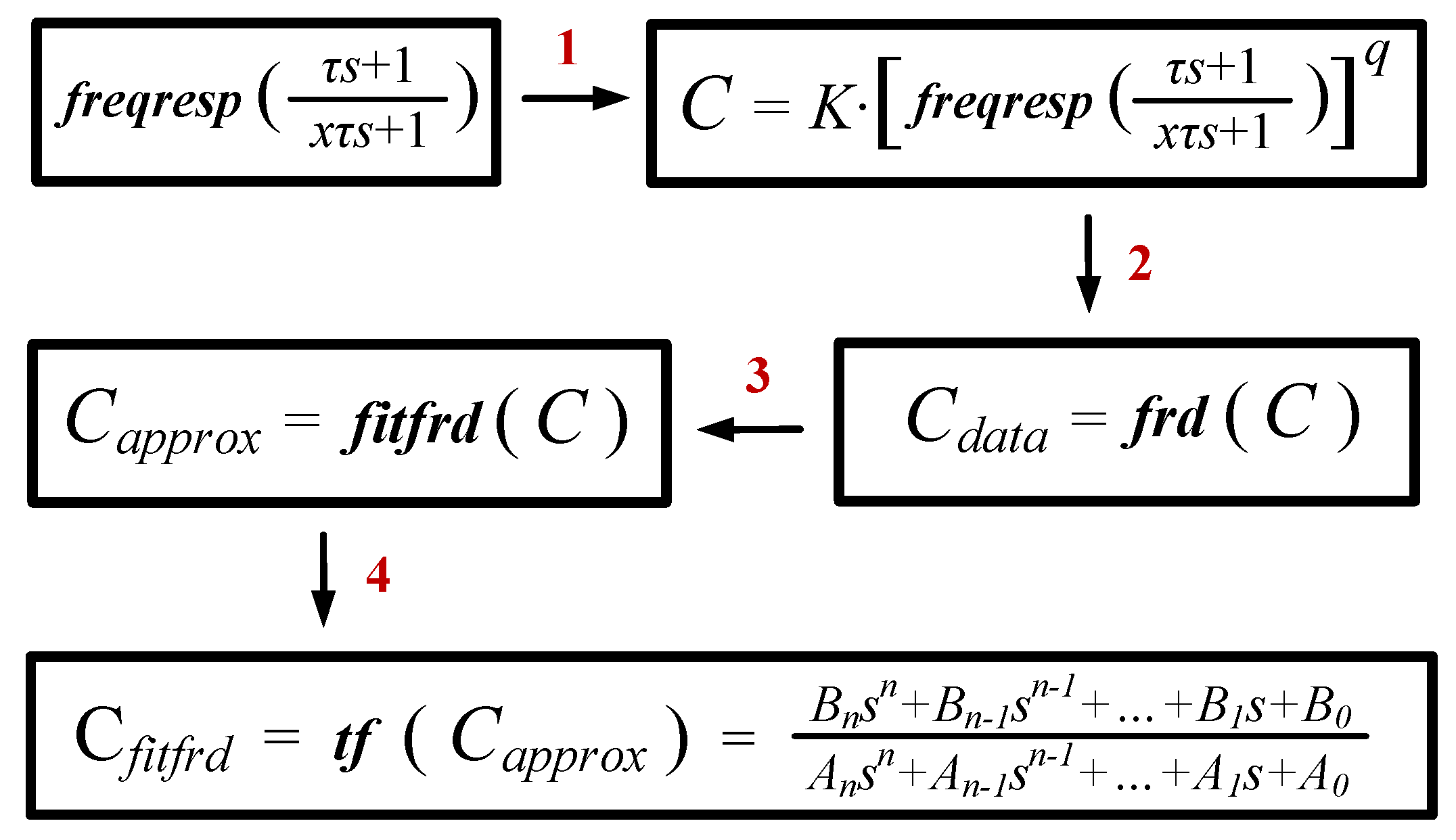
2. Curve-Fitting-Based Approximation of the Compensator Transfer Function

The approximation procedure is based on MATLAB software (ManthWorks, Natick, MA, USA) and the built-in functions it provides. Following the floating chart in Figure 1, a clear view of the approximation process is obtained. The starting point is the derivation of the frequency response data (both magnitude and phase) of the operator τ s + 1 / x τ s + 1 using the built-in function freqresp. Then, these data are raised to the fractional power q and multiplied by the low-frequency gain factor K; after that, the frequency response data model is formed utilizing the built-in function frd. The approximation process is performed by applying the fitfrd function to the frequency response data model—a procedure that is based on the Sanathanan–Koerner (SK) least square iterative method and fits the frequency response data into a state-space model [20,21,22,23,24]. A corresponding rational integer-order transfer function is derived using the tf command and has the form of a ratio of integer-order polynomials given by (5)
C f i t f r d s = B n s n + B n 1 s n 1 + , + B 1 s + B 0 A n s n + A n 1 s n 1 + , + A 1 s + A 0 ,
where A i and B i i = 0 n are positive, real coefficients.
The performance of the approximation, performed through the aforementioned method, will be compared with that offered by the Padé approximation. For this purpose, let us consider a car suspension system, which is described by the transfer function
P ( s ) = 1 M · s 2 ,
where M is the mass supported by each wheel, which is assumed to be equal to the fourth of total vehicle weight, lying in the range 100 , 900 kg [25]. Setting the gain crossover frequency for the typical mass of M o = 300 kg equal to ω c g = 10 rad/s to maximize passenger comfort and restricting the step response overshoot equal to 20% for all values of M, the resulting transfer function of the required FO lead compensator is
C ( s ) = 4260 · 1 + s 0.5 1 + s 200 0.65 .
Comparing (2) with (7), it is readily obtained that K = 4260 , ω p = 20 · ω c g = 200 rad/s and ω z = ω c g / 20 = 0.5 rad/s.
Considering a fourth-order approximation, the corresponding transfer functions (scaled by the factor K) of the approximated compensator, derived using the curve-fitting-based procedure presented here, are given by
C f i t f r d ( s ) = 49.040 s 4 + 5157 s 3 + 9.802 · 10 4 s 2 + 3.539 · 10 5 s + 1.974 · 10 5 s 4 + 233.3 s 3 + 1.14 · 10 4 s 2 + 1.16 · 10 5 s + 1.941 · 10 5 .
The corresponding transfer function, based on the Padé approximation method, is also obtained using MATLAB and its built-in function pade and is given by
C p a d e ( s ) = 47.540 s 4 + 3146 s 3 + 4.162 · 10 4 s 2 + 1.273 · 10 5 s + 7.009 · 10 4 s 4 + 181.6 s 3 + 5938 s 2 + 4.448 · 10 4 s + 6.783 · 10 4 .
The integer-order transfer function derived through the Oustaloup filter approximation is
C o u s t ( s ) = 49.130 s 4 + 3669 s 3 + 4.963 · 10 4 s 2 + 1.386 · 10 5 s + 7.009 · 10 4 s 4 + 197.7 s 3 + 7081 s 2 + 5.234 · 10 4 s + 7.009 · 10 4 .
A comparison between the two methods can be performed considering the gain and phase frequency responses in Figure 2a, where the ideal responses described by the transfer function in (7) are also shown by dashes. The associated error plots are given in Figure 2b, where it is concluded that the curve-fitting approximation method provides a more accurate approximation of the compensator transfer function than that offered by the Oustaloup and Padé approximations.

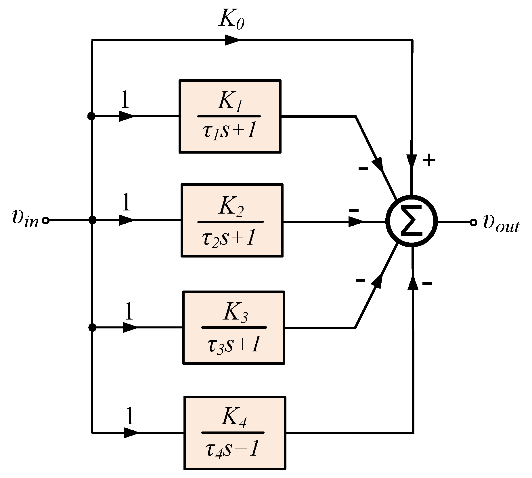
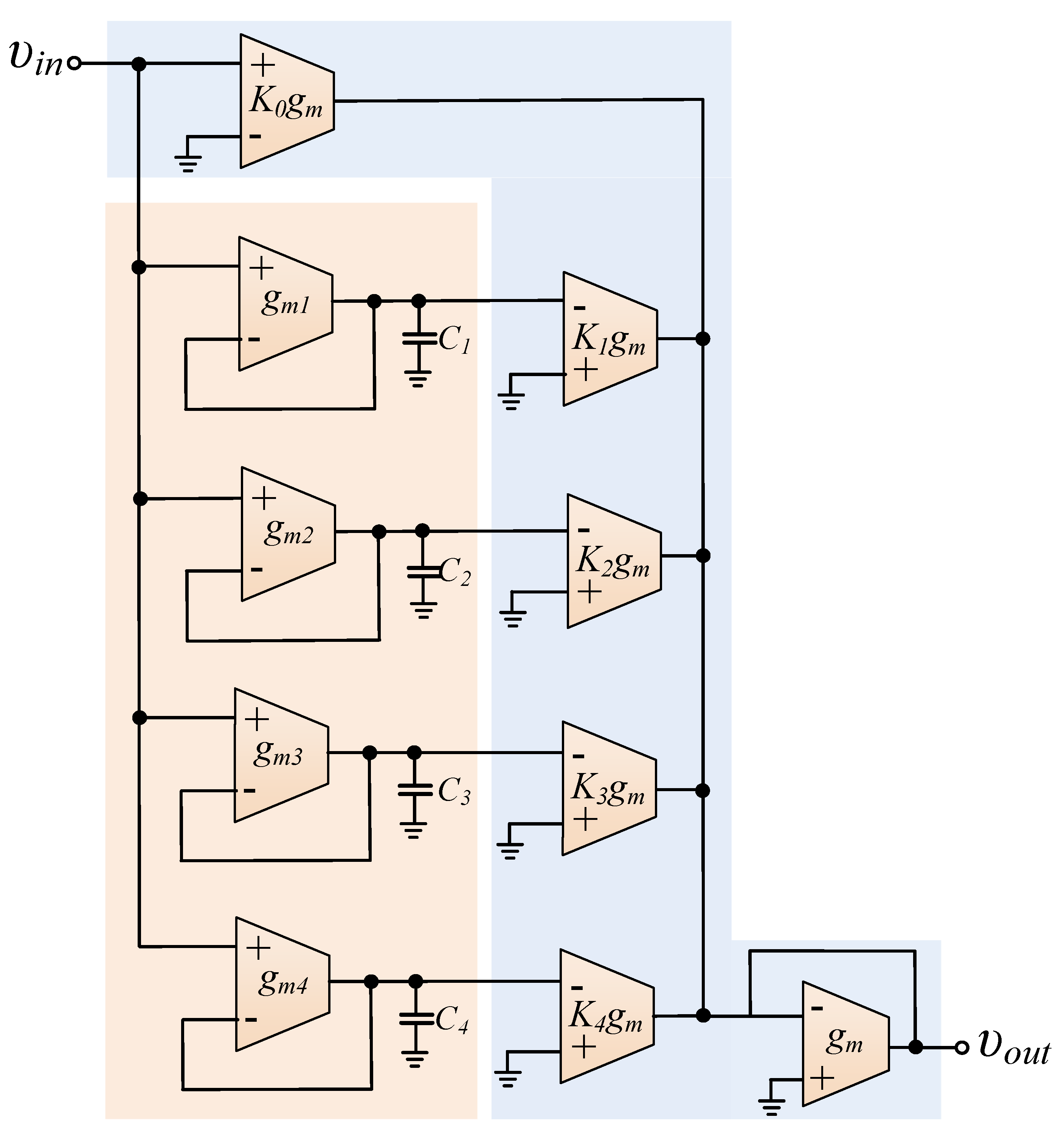
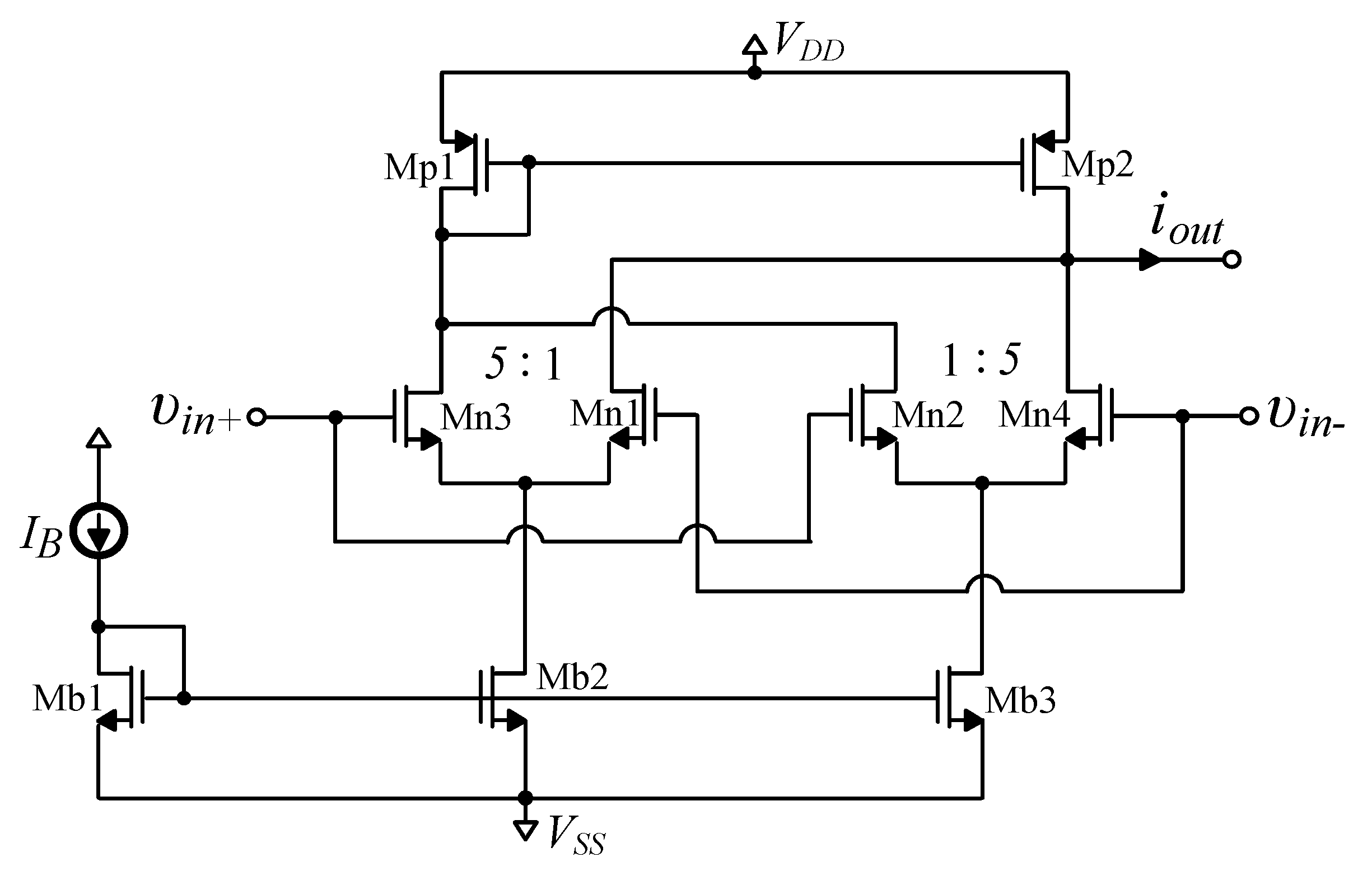
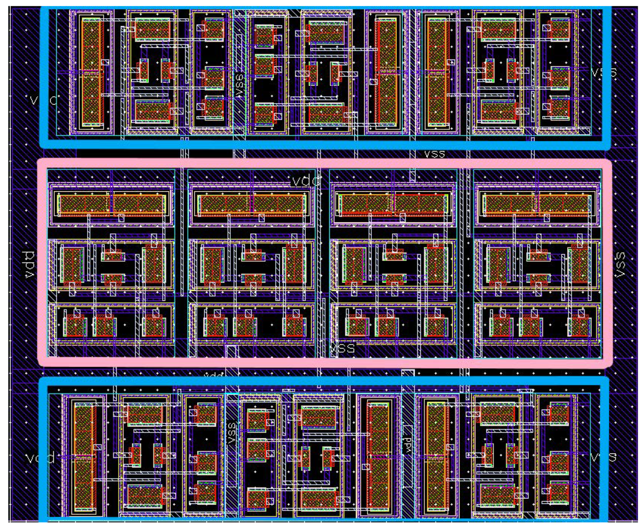
3. Implementation of the Approximated Compensator

The transfer function in (8) can be implemented using a multi-feedback topology, as presented in [26], or the partial fraction expansion method introduced in [27]. The last approach can be rewritten in the form of
C f i t f r d - p a r t i a l ( s ) = 49.044 33.780 0.0059 s + 1 9.840 0.0201 s + 1 3.328 0.0910 s + 1 1.074 0.4809 s + 1 .
The corresponding Functional Block Diagram (FBD) is demonstrated in Figure 3, where the implemented transfer function is as follows:
H s = K 0 K 1 1 + τ 1 s K 2 1 + τ 2 s K 3 1 + τ 3 s K 4 1 + τ 4 s .
Comparing the coefficients of (11) and (12), the derived values of scaling factors and time constants are summarized in Table 1.
The implementation of the FBD in Figure 3 is performed using Operational Transconductance Amplifiers (OTAs) as active elements because of the offered flexibility for performing the required inversion of the transfer functions originating from their differential input. The corresponding OTA-C implementation is demonstrated in Figure 4, while the OTA structure employed in the simulations is depicted in Figure 5 [28,29]. The expression of the transconductance of the OTA is given in (13):
g m = 5 9 · I B n · V T ,
where n is the slope factor of a MOS transistor in the sub-threshold region ( 1 < n < 2 ), V T is the thermal voltage (26 mV at 27 °C), and I B is the associated DC bias current. The time constants of integrators are electronically controlled through the bias current, and the required scaling factors are implemented through an appropriate scaling of the DC bias currents of the associated transconductances.
The implemented time constants are given by (14):
τ i = C i g m i .
Setting the DC bias current of OTAs equal to 30 pA , the calculated values of capacitors, obtained using (13) and (14) and the results in Table 1, are the following: C 1 = 3.13 pF , C 2 = 10.67 pF , C 3 = 48.51 pF , and C 4 = 256.18 pF . Utilizing the OTA-C structure in Figure 4 and considering the expression in (13), the compensator can be controlled using the DC currents.
Using the MOS transistor parameters provided by the AMS 0.35 μm CMOS Design Kit and considering power supply voltages V D D = V S S = 0.75 V , the aspect ratios of the MOS transistors of the circuit in Figure 5 for ensuring operation in the sub-threshold region are as follows: M p 1 M p 2 = 5 μ m / 15 μ m , M n 1 M n 2 = 2 μ m / 5 μ m , M n 3 M n 4 = 10 μ m / 5 μ m and M b 1 M b 3 = 5 μ m / 5 μ m .

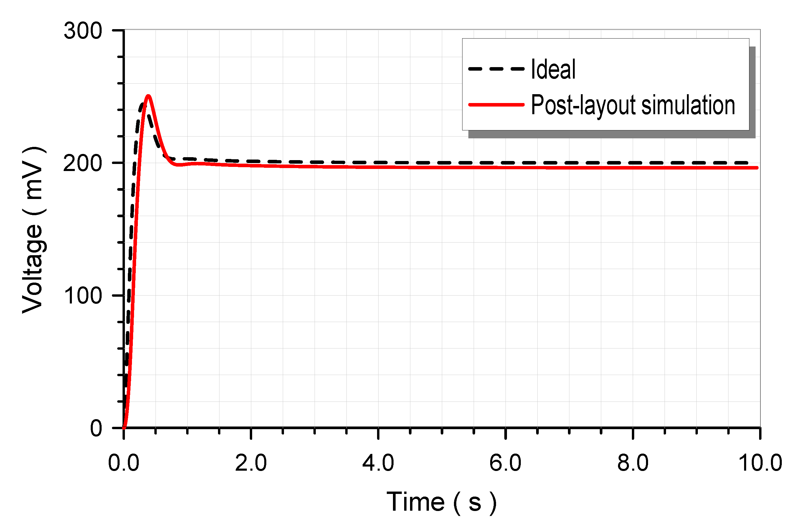
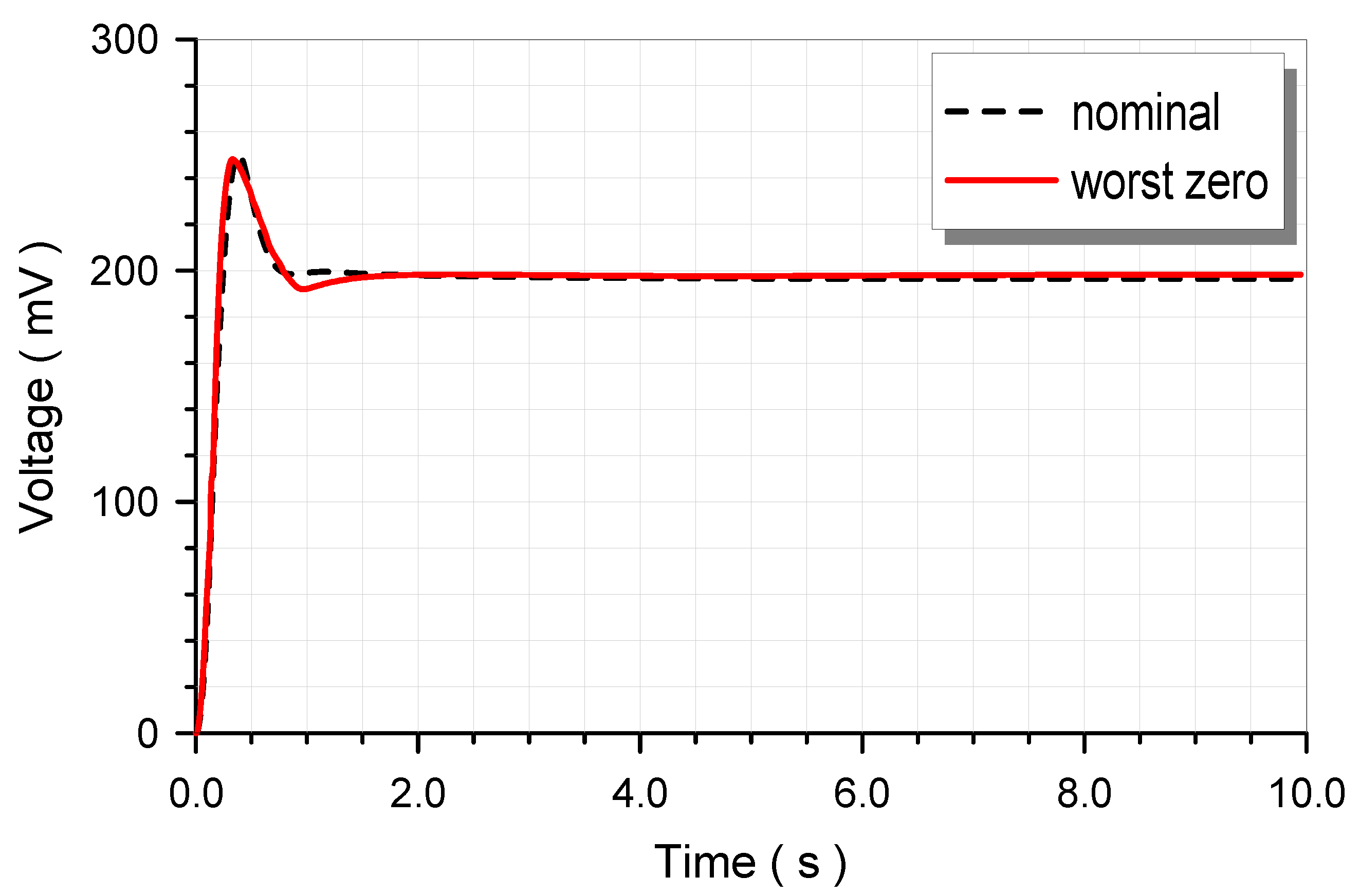
4. Simulation Results

The layout design of the compensator, performed using the Virtuoso Layout Editor of the Cadence IC design suite, is depicted in Figure 6 with dimensions of 190.65 μm × 156.55 μm.
The open-loop post-layout gain and phase responses of the system compensator-plant, obtained through the Virtuoso Analog Design Environment of Cadence software, are demonstrated in Figure 7a, along with the theoretically predicted responses given by dashes. The gain crossover frequency ω c g was 10 rad / s , as theoretically expected, and the phase margin was equal to 52.6 ° , with the theoretically predicted value being 55 ° . The corresponding closed-loop responses are given in Figure 7b. The time-domain behavior is evaluated through the stimulation of the system by a 200 mV step signal, and the output waveform is plotted in Figure 8. The theoretical settling time is 572.5 ms and the overshoot is 22.2 % , while the post-layout settling time is 625.8 ms and the overshoot is 25 % .
The robustness of the step response of the system is evaluated through PVT corner analysis, offered by the Analog Design Environment, considering temperatures of 0 °C, 27 °C and 60 °C and ±5% changes in the power supply voltages. The worst case waveform corresponds to the MOS transistors’ “worst-zero” models, and it is plotted in Figure 9. The measured settling time and overshot values were 534.1 ms and 24.8%, respectively, and these results confirm that the system has reasonable sensitivity characteristics.

5. Conclusions

The utilization of a curve-fitting-based approximation procedure for implementing a lead compensator for a car suspension system offers a more efficient approximation of the original fractional-order transfer function compared to the corresponding values achieved through the Oustaloup and Padé approximations. The proposed procedure offers design versatility, in the sense that it can be applied for implementing compensators of any type (i.e., lead and lag) and any order. Another attractive feature is that the implementation of the derived rational integer-order transfer function can be performed using any of the already known design techniques, including multi-feedback structures or a cascade connection of intermediate filter functions [30,31,32,33]. In addition, there is no restriction regarding the choice of the active elements; for example, operational amplifiers (op-amps), second generation current conveyors (CCIIs), Current Feedback Operational Amplifiers (CFOAs) or Field-Programmable Analog Arrays (FPAAs) [34] could be utilized for this purpose. Drawbacks of the proposed procedure are the requirement of multiple steps as well as its association with the MATLAB software, in contrast to the one-step Oustaloup and Padé approximation tools, which are not exclusively oriented to this software.

Author Contributions

Conceptualization, C.P. and J.B.; methodology, S.K.; software, E.M.; validation, E.M. and S.K.; formal analysis, C.P., J.B. and W.B.; investigation, C.P., S.K., J.B., W.B., A.T. and P.P.; writing—original draft preparation, E.M. and S.K.; writing—review and editing, C.P., J.B. and W.B.; project administration, C.P. and J.B. All authors have read and agreed to the published version of the manuscript.

Funding

This work was funded by the NAWA Polish National Agency for the Academic Exchange project “Science without borders. Establishing the framework for the long-term international cooperation of academic environments”, contract no. PPI/APM/2018/1/00049/U/001.

Institutional Review Board Statement

Not applicable.

Informed Consent Statement

Not applicable.

Data Availability Statement

No new data were created or analyzed in this study. Data sharing is not applicable to this article.

Acknowledgments

This research is co-financed by Greece and the European Union (European Social Fund-ESF) through the Operational Program “Human Resources Development, Education and Lifelong Learning” in the context of the project “Strengthening Human Resources Research Potential via Doctorate Research-2nd Cycle” (MIS-5000432), implemented by the State Scholarships Foundation (IKY). This article is based upon work from COST Action CA15225, a network supported by COST (European Cooperation in Science and Technology).

Conflicts of Interest

The authors declare no conflict of interest.

Abbreviations

The following abbreviations are used in this manuscript:
AMSAustria Mikro Systeme
CMOSComplementary metal oxide semiconductor
CCIISecond generation current conveyor
FOFractional-order
FBDFunctional block diagram
ICIntegrated circuit
IOInteger-order
MOSMetal oxide semiconductor
OTAOperational transconductance amplifier
PFEPartial fraction expansion

References

  1. Oustaloup, A.; Moreau, X.; Nouillant, M. The CRONE suspension. Control Eng. Pract. 1996, 4, 1101–1108. [Google Scholar] [CrossRef]
  2. Aldair, A.A.; Wang, W.J. Design of fractional order controller based on evolutionary algorithm for a full vehicle nonlinear active suspension systems. Int. J. Control Autom. 2010, 3, 33–46. [Google Scholar]
  3. Taksale, A.S. Modeling, Analysis and Control of Passive and Active Suspension System for a Quarter Car. Int. J. Appl. Eng. Res. 2013, 8, 1405–1414. [Google Scholar]
  4. Dong, X.; Zhao, D.; Yang, B.; Han, C. Fractional-order control of active suspension actuator based on parallel adaptive clonal selection algorithm. J. Mech. Sci. Technol. 2016, 30, 2769–2781. [Google Scholar] [CrossRef]
  5. Baig, W.M.; Hou, Z.; Ijaz, S. Fractional order controller design for a semi-active suspension system using Nelder-Mead optimization. In Proceedings of the 2017 29th Chinese Control And Decision Conference (CCDC), Chongqing, China, 28–30 May 2017; pp. 2808–2813. [Google Scholar] [CrossRef]
  6. Chen, Y.D. Study on Active Suspension with Variable Structure Control Based on the Fractional Order Exponential Reaching Law. In Applied Mechanics and Materials; Trans Tech Publ: Baech, Switzerland, 2017; Volume 872, pp. 337–345. [Google Scholar]
  7. Kumar, V.; Rana, K.; Kumar, J.; Mishra, P. Self-tuned robust fractional order fuzzy PD controller for uncertain and nonlinear active suspension system. Neural Comput. Appl. 2018, 30, 1827–1843. [Google Scholar] [CrossRef]
  8. You, H.; Shen, Y.; Xing, H.; Yang, S. Optimal control and parameters design for the fractional-order vehicle suspension system. J. Low Freq. Noise Vib. Act. Control 2018, 37, 456–467. [Google Scholar] [CrossRef] [Green Version]
  9. Swethamarai, P.; Lakshmi, P. Adaptive-Fuzzy Fractional Order PID Controller-Based Active Suspension for Vibration Control. IETE J. Res. 2020, 2020, 1–16. [Google Scholar] [CrossRef]
  10. Nguyen, S.D.; Lam, B.D.; Choi, S.B. Smart dampers-based vibration control–Part 2: Fractional-order sliding control for vehicle suspension system. Mech. Syst. Signal Process. 2021, 148, 107145. [Google Scholar] [CrossRef]
  11. Monje, C.A.; Calderon, A.J.; Vinagre, B.M.; Feliu, V. The fractional order lead compensator. In Proceedings of the Second IEEE International Conference on Computational Cybernetics, 2004. ICCC 2004, Vienna, Austria, 30 August–1 September 2004; pp. 347–352. [Google Scholar]
  12. Tavazoei, M.S.; Tavakoli-Kakhki, M. Compensation by fractional-order phase-lead/lag compensators. IET Control Theory Appl. 2014, 8, 319–329. [Google Scholar] [CrossRef]
  13. Vinagre, B.M.; Monje, C.A.; Calderón, A.J.; Suárez, J.I. Fractional PID controllers for industry application. A brief introduction. J. Vib. Control 2007, 13, 1419–1429. [Google Scholar] [CrossRef]
  14. Jadhav, S.P.; Hamde, S.T. A simple method to design robust fractional-order lead compensator. Int. J. Control Autom. Syst. 2017, 15, 1236–1248. [Google Scholar] [CrossRef]
  15. Dastjerdi, A.A.; Vinagre, B.M.; Chen, Y.; HosseinNia, S.H. Linear fractional order controllers; A survey in the frequency domain. Annu. Rev. Control 2019, 47, 51–70. [Google Scholar] [CrossRef]
  16. Monje, C.A.; Vinagre, B.M.; Calderon, A.J.; Feliu, V.; Chen, Y. Auto-tuning of fractional lead-lag compensators. IFAC Proc. Vol. 2005, 38, 319–324. [Google Scholar] [CrossRef]
  17. Monje, C.A.; Chen, Y.; Vinagre, B.M.; Xue, D.; Feliu-Batlle, V. Fractional-Order Systems and Controls: Fundamentals and Applications; Springer Science & Business Media: Berlin/Heidelberg, Germany, 2010. [Google Scholar]
  18. Oustaloup, A.; Levron, F.; Mathieu, B.; Nanot, F.M. Frequency-band complex noninteger differentiator: Characterization and synthesis. IEEE Trans. Circuits Syst. I Fundam. Theory Appl. 2000, 47, 25–39. [Google Scholar] [CrossRef]
  19. Lanusse, P.; Sabatier, J.; Gruel, D.N.; Oustaloup, A. Second and third generation crone control-system design. In Fractional Order Differentiation and Robust Control Design; Springer: Berlin/Heidelberg, Germany, 2015; pp. 107–192. [Google Scholar]
  20. Ozdemir, A.A.; Gumussoy, S. Transfer function estimation in system identification toolbox via vector fitting. IFAC Pap. 2017, 50, 6232–6237. [Google Scholar] [CrossRef]
  21. Bingi, K.; Ibrahim, R.; Karsiti, M.N.; Hassam, S.M.; Harindran, V.R. Frequency response based curve fitting approximation of fractional–order PID controllers. Int. J. Appl. Math. Comput. Sci. 2019, 29, 311–326. [Google Scholar] [CrossRef] [Green Version]
  22. Bingi, K.; Ibrahim, R.; Karsiti, M.N.; Hassan, S.M.; Harindran, V.R. Fractional-order Systems and PID Controllers; Springer: Berlin/Heidelberg, Germany, 2020. [Google Scholar]
  23. Maione, G. Design of Cascaded and Shifted Fractional-Order Lead Compensators for Plants with Monotonically Increasing Lags. Fractal Fract. 2020, 4, 37. [Google Scholar] [CrossRef]
  24. Kapoulea, S.; Psychalinos, C.; Elwakil, A.S. Power law filters: A new class of fractional-order filters without a fractional-order Laplacian operator. AEU Int. J. Electron. Commun. 2021, 129, 153537. [Google Scholar] [CrossRef]
  25. Raynaud, H.F.; Zergaınoh, A. State-space representation for fractional order controllers. Automatica 2000, 36, 1017–1021. [Google Scholar] [CrossRef]
  26. Dimeas, I.; Petras, I.; Psychalinos, C. New analog implementation technique for fractional-order controller: A DC motor control. AEU Int. J. Electron. Commun. 2017, 78, 192–200. [Google Scholar] [CrossRef]
  27. Bertsias, P.; Psychalinos, C.; Maundy, B.J.; Elwakil, A.S.; Radwan, A.G. Partial fraction expansion–based realizations of fractional-order differentiators and integrators using active filters. Int. J. Circuit Theory Appl. 2019, 47, 513–531. [Google Scholar] [CrossRef]
  28. Corbishley, P.; Rodriguez-Villegas, E. A nanopower bandpass filter for detection of an acoustic signal in a wearable breathing detector. IEEE Trans. Biomed. Circuits Syst. 2007, 1, 163–171. [Google Scholar] [CrossRef] [PubMed]
  29. Tsirimokou, G.; Psychalinos, C.; Elwakil, A. Design of CMOS Analog Integrated Fractional-Order Circuits: Applications in Medicine and Biology; Springer: Berlin/Heidelberg, Germany, 2017. [Google Scholar]
  30. Mohan, P.A. VLSI Analog Filters: Active RC, OTA-C, and SC; Springer Science & Business Media: Berlin/Heidelberg, Germany, 2012. [Google Scholar]
  31. Gonzalez, E.; Dorčák, L.; Monje, C.; Valsa, J.; Caluyo, F.; Petráš, I. Conceptual design of a selectable fractional-order differentiator for industrial applications. Fract. Calc. Appl. Anal. 2014, 17, 697–716. [Google Scholar] [CrossRef] [Green Version]
  32. Muñiz-Montero, C.; García-Jiménez, L.V.; Sánchez-Gaspariano, L.A.; Sánchez-López, C.; González-Díaz, V.R.; Tlelo-Cuautle, E. New alternatives for analog implementation of fractional-order integrators, differentiators and PID controllers based on integer-order integrators. Nonlinear Dyn. 2017, 90, 241–256. [Google Scholar] [CrossRef]
  33. Psychalinos, C. Development of fractional-order analog integrated controllers–application examples. Appl. Control 2019, 6, 357. [Google Scholar] [CrossRef]
  34. Silva-Juárez, A.; Tlelo-Cuautle, E.; de la Fraga, L.G.; Li, R. FPAA-based implementation of fractional-order chaotic oscillators using first-order active filter blocks. J. Adv. Res. 2020, 25, 77–85. [Google Scholar] [CrossRef]
Figure 1. Floating chart description of the curve-fitting-based approximation procedure for approximating the transfer function in (2).
Fractalfract 05 00046 g001
Figure 2. (a) Gain and phase frequency responses of the compensator derived from fitfrd (8), Padé (9), and Oustaloup (10) approximation methods along with the ideal responses derived from (7) and (b) the relative errors for each method.
Fractalfract 05 00046 g002
Figure 3. Functional Block Diagram implementing the transfer function in (11).
Fractalfract 05 00046 g003
Figure 4. OTA-C implementation of the approximated compensator.
Fractalfract 05 00046 g004
Figure 5. MOS circuitry of a high-linearity OTA, as employed in simulations.
Fractalfract 05 00046 g005
Figure 6. Layout design of the OTA-C structure in Figure 4 (the pink framed part corresponds to the integration stage, while the blue framed part represents the summation stage).
Fractalfract 05 00046 g006
Figure 7. Post-layout (a) open-loop and (b) closed-loop gain and phase frequency responses of the system compensator-plant.
Fractalfract 05 00046 g007
Figure 8. Post-layout step response of the closed-loop system stimulated by an input voltage of 200 mV.
Fractalfract 05 00046 g008
Figure 9. Worst-case step response of the system obtained through PVT corner analysis.
Fractalfract 05 00046 g009
Table 1. Values of scaling factors and time constants of the FBD in Figure 3.
Scaling FactorsTime Constants
VariableValueVariableValue
K 0 49.044
K 1 33.780 τ 1 (ms)5.9
K 2 9.840 τ 2 (ms)20.1
K 3 3.328 τ 3 (ms)91
K 4 1.074 τ 4 (ms)480.9
Publisher’s Note: MDPI stays neutral with regard to jurisdictional claims in published maps and institutional affiliations.

