Energy Mutual Aid Converter with Fractional-Order Model Predictive Control for Field Medical Electric Vehicles

Abstract

Although electric vehicles have been widely adopted in recent years, insufficient charging infrastructure in remote areas may still compromise the continuity of emergency operations involving field medical electric vehicles (EVs). Motivated by the need for temporary DC energy support from a donor vehicle to a field medical EV, this paper investigates an isolated DC–DC energy-sharing converter based on a series-resonant dual-active-bridge (SRDAB) topology and its associated control method. First, the SRDAB converter is employed to satisfy the requirements of low-voltage input, galvanic isolation, voltage step-up, and DC power transfer. Based on the fundamental harmonic approximation (FHA), a steady-state power relationship and a control-oriented dynamic model are derived to characterize the coupling between the phase-shift angle, transferred power, and output voltage. Subsequently, a fractional-order model predictive control strategy tuned offline using the grey wolf optimizer (GWO-FOMPC) is developed to address donor-side input-voltage variations, recipient-side equivalent-load disturbances, and the nonlinear power-transfer characteristics of the SRDAB converter. In this strategy, a fractional-order proportional–integral outer loop generates the reference transferred power, while a fractional-order predictive inner loop analytically determines the phase-shift command online. Finally, simulations and converter-level experiments validate the dynamic regulation performance of the proposed control strategy under emulated energy-sharing conditions for field medical EVs.

1. Introduction

In recent years, electric vehicles (EVs) have been widely adopted in transportation electrification and low-carbon mobility. However, limited battery capacity, long charging duration, and the uneven distribution of charging infrastructure may still restrict the operational continuity of EVs in remote areas and emergency missions [1]. For field medical EVs undertaking on-site medical treatment, casualty transportation, and emergency support, insufficient battery energy in areas far from fixed charging facilities may interrupt the execution of their assigned missions. Vehicle-to-vehicle (V2V) energy transfer enables a donor vehicle to provide temporary electrical energy directly to a recipient vehicle and can therefore serve as a supplementary solution when fixed charging facilities are unavailable [2]. Motivated by this application scenario, this paper investigates an isolated DC–DC energy-transfer interface and its dynamic control method for temporary dc energy support from a donor vehicle to a field medical EV.

Existing V2V energy-transfer solutions mainly include the reuse of vehicle propulsion systems, the reuse of onboard chargers, dedicated power-conversion interfaces, and wireless power transfer. Umesh et al. realized direct power transfer between EVs by utilizing the traction-motor windings and drivetrain converters, thereby reducing the requirement for additional power devices; however, this method requires reconfiguration of the original vehicle propulsion system [3]. Shafiqurrahman et al. achieved EV-to-EV energy transfer by reusing the existing onboard converters, although the applicability of this method depends on the original charging topology and interface configuration of the vehicles [4]. Wang et al. developed a fast charging control method for V2V energy-transfer devices and improved the dynamic response of the charging process, whereas the study primarily focused on charging control rather than the internal nonlinear power regulation of an isolated converter [2]. Xie et al. investigated a strongly coupled wireless V2V charging system with constant-current and constant-voltage output characteristics; nevertheless, wireless solutions require additional consideration of the coupling mechanism, vehicle alignment, and mutual-inductance variations [5]. Qiu and Khadkikar further utilized a motor inverter and motor windings to realize V2V energy transfer, but this approach also relies on the hardware configuration of the vehicle traction system [6]. A recent review indicated that practical V2V energy transfer requires coordinated consideration of the power interface, communication protocol, and vehicle energy-management system [1]. Therefore, for temporary energy-support scenarios in which modification of the original vehicle propulsion system is undesirable, an external DC–DC conversion interface with galvanic isolation and independent control capability remains worthy of investigation.

Isolated dual-active-bridge (DAB) converters have been widely employed in EV and dc-distribution applications because of their high-frequency galvanic isolation, bidirectional power-transfer capability, and high power density [7]. To reduce the circulating current and current stress of DAB converters over a wide voltage range, Li et al. proposed a hybrid five-variable modulation method that minimizes the root-mean-square current [8]. He et al. systematically reviewed the modeling, modulation, and control methods of DAB converters and indicated that variations in operating conditions significantly affect the power-transfer characteristics and soft-switching range [9]. The series-resonant dual-active-bridge (SRDAB) converter introduces a resonant network into the power-transfer path and combines the resonant impedance with a high-frequency transformer to realize isolated voltage conversion and dc energy transfer. Zhou et al. developed a total-loss-minimization method for an SRDAB converter under triple-phase-shift modulation, with an emphasis on steady-state loss reduction and modulation-parameter optimization [10]. Recent studies have further improved the efficiency of SRDAB converters through resonant-parameter design and operating-point optimization, whereas output-voltage regulation under dynamic disturbances has received relatively limited attention [11]. Accordingly, most existing SRDAB studies have focused on steady-state efficiency, current-stress reduction, and soft-switching performance, while closed-loop dynamic control under input-voltage variations and load disturbances requires further investigation.

Under single-phase-shift modulation, the phase-shift angle of an SRDAB converter first changes the resonant current and transferred power, whereas the output voltage is jointly determined by the transferred power, output capacitor, and load. Consequently, an indirect and nonlinear relationship exists between the control input and output voltage. Zhao et al. improved the phase-shift control of a DAB converter using a power-based model, thereby enhancing the dynamic response under operating-point variations [12]. Tarisciotti et al. applied finite-control-set model predictive control to a DAB converter, allowing the switching state to be directly selected according to the predictive control objective [13]. Zhu et al. combined parameter identification with model predictive control to reduce the influence of inductance-parameter mismatch on predictive performance [14]. Sun et al. proposed a model-free moving-discretized-control-set predictive method, which reduced the dependence of predictive control on an accurate converter model [15]. Li et al. combined a super-twisting observer with sensitivity analysis to enhance the robustness of DAB model predictive control against disturbances and model uncertainties [16]. Kong et al. incorporated current-stress minimization and soft-switching requirements into the predictive control objective, thereby coordinating the dynamic response and converter operating conditions [17]. These studies demonstrate the suitability of model predictive control for multivariable and constrained control of DAB converters. Nevertheless, most existing methods employ integer-order predictive models and mainly focus on conventional DAB topologies or switching-state optimization.

Fractional-order control introduces non-integer-order differential or integral operators, enabling the controller to utilize historical state information over a finite interval and providing additional flexibility in parameter tuning. Ke et al. applied a fractional-order predictive model to power converters and demonstrated that the finite-memory term can improve dynamic regulation under parameter variations and external disturbances [18]. Long et al. developed a fractional-order sequential model predictive control method for T-type converters, further demonstrating the feasibility of fractional-order predictive structures in power electronic systems [19]. Albalawi et al. incorporated fractional-order operators into model-free predictive voltage control for voltage-source inverters, demonstrating the applicability of fractional-order predictive structures to converter voltage regulation [20]. Peng et al. employed the grey wolf optimizer (GWO) to coordinately tune the parameters of a fractional-order predictive controller for a Boost converter, thereby facilitating the design of a multi-parameter control system [21]. However, existing studies have mainly focused on Boost, T-type, and other power converters, without fully considering the indirect nonlinear coupling among the phase-shift angle, resonant transferred power, and output voltage of an SRDAB converter. Moreover, incorporating finite-memory characteristics into a control-oriented SRDAB model and rapidly calculating the control command subject to phase-shift constraints require further investigation.

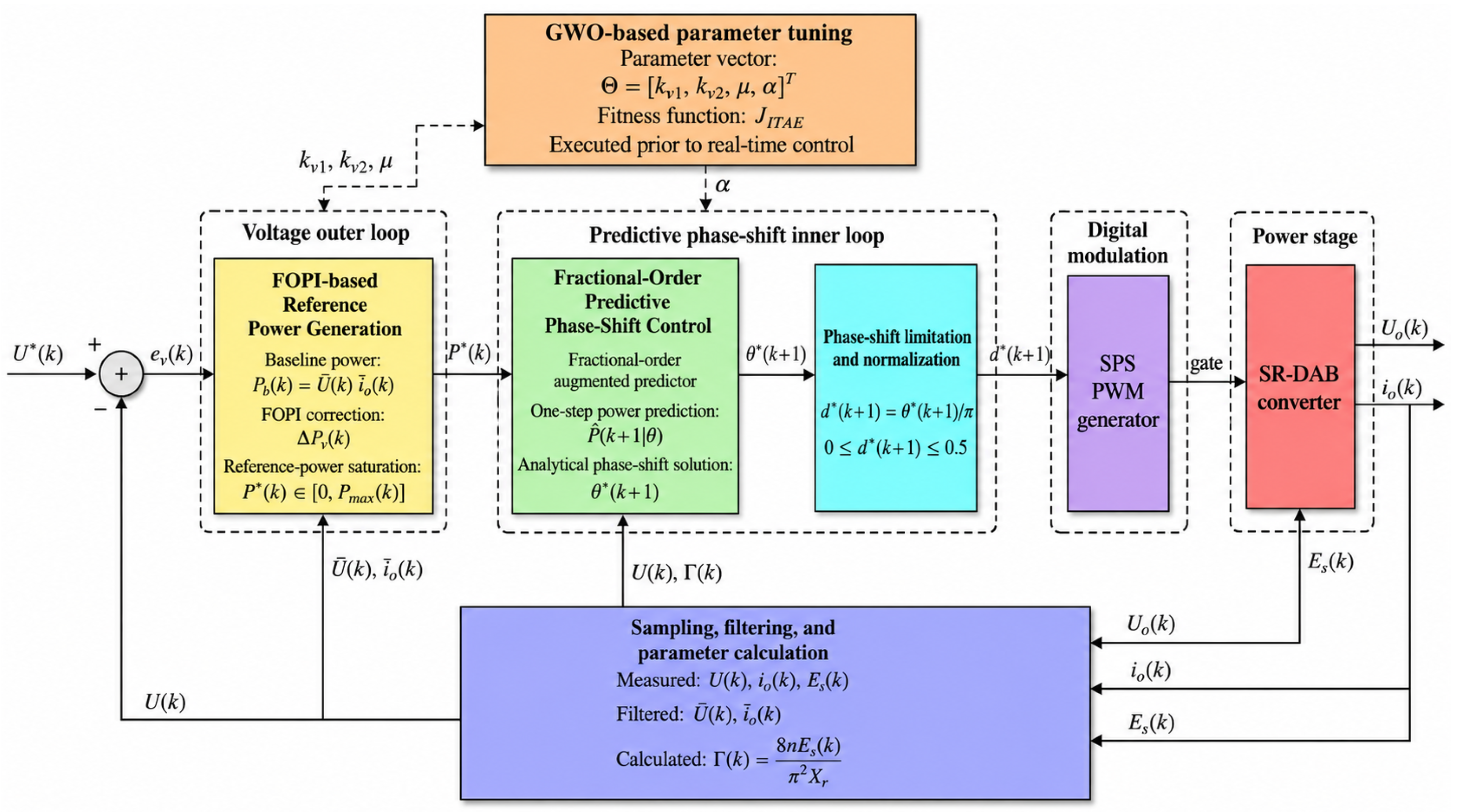
To address the above issues, this paper investigates an SRDAB-based isolated DC–DC energy-transfer converter and its fractional-order model predictive control method, with temporary dc energy support from a donor vehicle to a field medical EV considered as the application background. The overall converter configuration and signal paths are illustrated in Figure 1.

The main contributions of this paper are summarized as follows:

• To address the need for temporary energy support for field medical electric vehicles in areas with limited access to fixed charging facilities, an isolated DC energy-sharing system based on a series-resonant dual-active-bridge (SRDAB) converter is investigated. The steady-state power-transfer relationship and a control-oriented dynamic model are derived using the fundamental harmonic approximation. The nonlinear coupling between the phase-shift angle, resonant power, resonant current, and output voltage is analyzed, providing a modeling basis for controller design and dynamic-performance evaluation.
• To improve the dynamic regulation capability of conventional integer-order model predictive control under successive operating-condition variations, a dual-loop fractional-order model predictive control structure is developed. The outer-loop fractional-order proportional–integral controller generates the reference power, while the inner predictive loop introduces fractional-order finite-memory weighting into the integer-order physical model and analytically calculates the constrained phase-shift angle according to the power-tracking error. The finite-memory formulation incorporates historical information into the prediction process while avoiding online iterative optimization. When the fractional order is set to unity, the finite-memory predictor reduces to its corresponding integer-order form.
• To address the difficulty of manually tuning multiple controller parameters across different operating conditions, the grey wolf optimizer is employed offline to determine the fractional orders, controller gains, and associated prediction parameters. No population-based optimization is performed during real-time converter operation. Comparative simulations are conducted under variations in input voltage, load resistance, and output-voltage reference, followed by experimental comparisons between IOMPC and GWO-FOMPC on an SRDAB prototype. The control performance is evaluated in terms of settling time, response to parameter mismatch, real-time computational burden, memory requirement, and steady-state efficiency.

The remainder of this paper is organized as follows. Section 2 introduces the operating principle and mathematical model of the SRDAB converter. Section 3 presents the proposed GWO-FOMPC strategy. Section 4 and Section 5 report the simulation and experimental results, respectively. Finally, Section 6 concludes the paper.

2. Modeling and Power-Transfer Characteristics of the SRDAB Converter

2.1. Topology, Transformer Convention, and Operating Assumptions

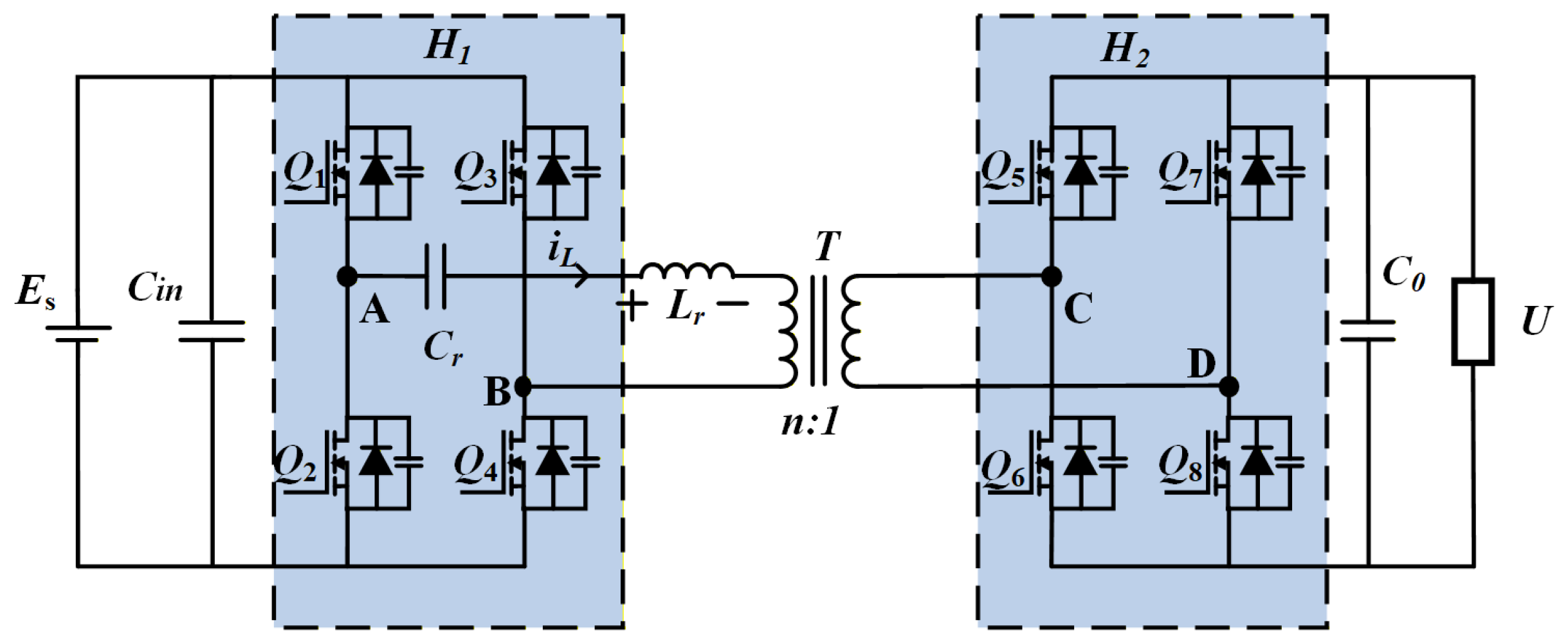
The converter investigated in this paper is an isolated DC–DC SRDAB converter for V2V emergency energy transfer. The topology consists of an input-side full bridge, a series resonant inductor $L_r$, a series resonant capacitor $C_r$, a high-frequency isolation transformer, a output-side full bridge and an output filter stage.

The input dc voltage, output voltage, output current and equivalent load resistance are denoted by $E_s$, U, $i_o$ and R, respectively. The transformer turn ratio is defined as

$$n={\displaystyle \frac{N_p}{N_s}},$$

(1)

where $N_p$ and $N_s$ denote the turns on the primary and secondary-sides, respectively. Therefore, the transformer is labeled $n:1$ in Figure 2. Under this convention, the output voltage referred to the primary side is

$$U^{\prime }=nU,$$

(2)

and the output load resistance referred to the primary side is

$$R_e=n^{2}R.$$

(3)

Positive power is defined as power transferred from the input-to-output bridge. Although the SRDAB topology is capable of bidirectional power transfer, the proposed controller is evaluated in this paper for the forward donor-to-recipient charging mode.

The following assumptions are adopted in the analytical model:

• Switching devices are regarded as ideal, and switching transients are neglected.
• The transformer magnetizing current is neglected, and the leakage inductance is included in $L_r$.
• The output capacitor is sufficiently large so that the output-voltage variation within one switching period is negligible.
• The bridge voltages are represented by their fundamental components using the fundamental harmonic approximation (FHA).
• The switching frequency is selected above the resonant frequency, i.e., $f_s>f_r$, so that the equivalent resonant reactance is positive.

The assumptions above separate the switching-scale resonant behavior from the low-frequency output-voltage dynamics. At the nominal operating point, $f_s=100\mathrm{kHz}$ and $f_r\approx 80\mathrm{kHz}$, giving the normalized frequency ${\lambda }_f=f_s/f_r=1.25$. The converter therefore operates above resonance, and the series-resonant branch presents a positive equivalent reactance at the switching frequency. In addition, the resonant tank attenuates the high-order harmonic components of the bridge voltages, so that the resonant current is dominated by its fundamental component. This property supports the use of the fundamental bridge-voltage components in the derivation of the resonant current and transferred power.

At the nominal load, the output-side time constant is ${\tau }_o=R{C}_o=25\times 470\mathsf{\mu }\mathrm{F}=11.75\mathrm{ms}$, which is substantially larger than the switching period $T_s=10\mathsf{\mu }\mathrm{s}$. The output voltage can consequently be regarded as constant over one switching period, while its low-frequency evolution is described by the averaged capacitor-current balance. Accordingly, the resonant path is represented by its fundamental-frequency phasor relation, and the output stage is represented by its averaged voltage dynamics. The dependence of the resulting model coefficients on $L_r$, $C_r$, $C_o$, and R is derived in Section 2.6.

As shown in Figure 2, the two full bridges are coupled through the resonant tank and the high-frequency transformer. The series resonant branch can reduce current stress and facilitate soft-switching operation, making the topology suitable for isolated power transfer in the V2V charging scenario.

2.2. Operating Waveforms Under SPS Control

Under single-phase-shift (SPS) modulation, both full bridges operate with a duty ratio of $50\%$. The phase displacement between the two bridge voltages is denoted by $\theta$. The normalized phase-shift ratio is defined as

$$d={\displaystyle \frac{\theta }{\pi }},0\le d\le 0.5.$$

(4)

For the forward donor-to-recipient power-transfer mode considered in this paper,

$$0\le \theta \le {\displaystyle \frac{\pi }{2}}.$$

(5)

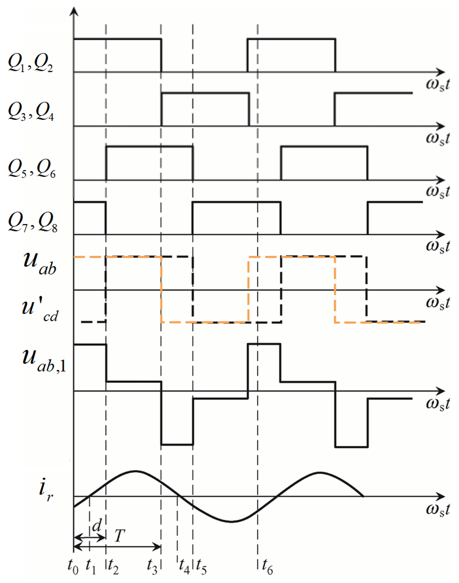
Figure 3 shows the typical operating waveforms under SPS control. The phase displacement between the input-side and output-side bridge voltages determines the equivalent driving voltage imposed on the resonant tank. As $\theta$ increases, the resonant-current amplitude and transferred power increase. Conversely, a smaller $\theta$ reduces the transferred power.

The phase-shift angle does not directly regulate the output voltage. Instead, it first regulates the transferred power and resonant current, after which the output voltage is established through the output filter and load dynamics. Therefore, it is physically meaningful for the outer loop to generate a reference transferred power and for the inner loop to determine the corresponding phase-shift command.

2.3. Steady-State Modeling Based on the Fundamental Harmonic Approximation

The resonant angular frequency and resonant frequency are defined as

$${\omega }_r={\displaystyle \frac{1}{\sqrt{L_r{C}_r}}},$$

(6)

$$f_r={\displaystyle \frac{{\omega }_r}{2\pi }},$$

(7)

respectively. Let $f_s$ denote the switching frequency. The normalized switching frequency is

$${\lambda }_f={\displaystyle \frac{f_s}{f_r}}.$$

(8)

The quality factor is defined as

$$Q={\displaystyle \frac{{\omega }_r{L}_r}{R_e}}={\displaystyle \frac{{\omega }_r{L}_r}{n^{2}R}}.$$

(9)

At the angular switching frequency ${\omega }_s=2\pi f_s$, the equivalent reactance of the series resonant tank is

$$X_r={\omega }_s{L}_r-{\displaystyle \frac{1}{{\omega }_s{C}_r}}.$$

(10)

The normalized resonant reactance is

$$x_r={\displaystyle \frac{X_r}{R_e}}=Q\left({\lambda }_f-{\displaystyle \frac{1}{{\lambda }_f}}\right).$$

(11)

The primary-referred voltage ratio is defined as

$$M={\displaystyle \frac{nU}{E_s}}.$$

(12)

It should be noted that the actual dc voltage gain is $U/E_s=M/n$.

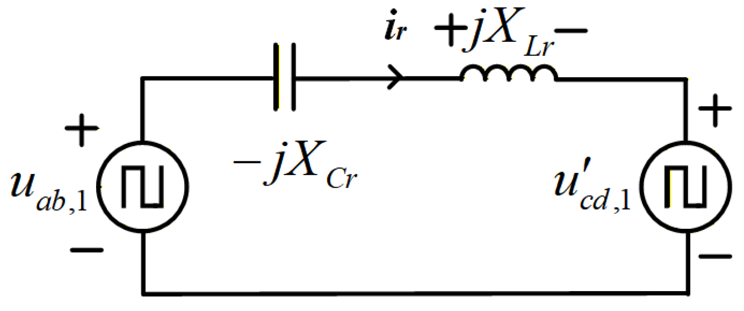
The resulting FHA-based AC equivalent circuit is shown in Figure 4.

Using FHA, the fundamental components of the input-side and output-side bridge voltages are expressed as

$$u_{ab,1}\left(t\right)={\displaystyle \frac{4E_s}{\pi }}sin\left({\omega }_{s}t\right),$$

(13)

$$u_{cd,1}^{\prime }\left(t\right)={\displaystyle \frac{4nU}{\pi }}sin({\omega }_{s}t-\theta )={\displaystyle \frac{4M{E}_s}{\pi }}sin({\omega }_{s}t-\theta ).$$

(14)

The corresponding peak-value phasors are

$${\underline{U}}_{ab,1}={\displaystyle \frac{4E_s}{\pi }}\angle 0,$$

(15)

$${\underline{U}}_{cd,1}^{\prime }={\displaystyle \frac{4nU}{\pi }}\angle (-\theta ).$$

(16)

Therefore, the resonant-current phasor is

$${\underline{I}}_r={\displaystyle \frac{{\underline{U}}_{ab,1}-{\underline{U}}_{cd,1}^{\prime }}{j{X}_r}}.$$

(17)

The time-domain resonant current can be approximated as

$$i_r\left(t\right)={\displaystyle \frac{4E_s}{\pi X_r}}\left[sin\left({\omega }_{s}t-{\displaystyle \frac{\pi }{2}}\right)-Msin\left({\omega }_{s}t-\theta -{\displaystyle \frac{\pi }{2}}\right)\right].$$

(18)

The resonant-current peak value is

$$I_{r,\mathrm{pk}}={\displaystyle \frac{4E_s}{\pi X_r}}\sqrt{1+M^2-2Mcos\theta }.$$

(19)

Assuming a near-sinusoidal resonant current, the corresponding RMS value is

$$I_{r,\mathrm{rms}}={\displaystyle \frac{I_{r,\mathrm{pk}}}{\sqrt{2}}}.$$

(20)

Equation (19) indicates that increasing $\theta$ improves the power-transfer capability but also increases resonant-current stress. This tradeoff motivates the predictive phase-shift optimization developed later.

2.4. Voltage Gain and Power-Transfer Characteristics

The average transferred power is calculated from the input-side fundamental voltage and resonant current:

$$P_t={\displaystyle \frac{1}{2}}\mathrm{Re}\left\{{\underline{U}}_{ab,1}{\underline{I}}_r^{*}\right\}.$$

(21)

Substituting (15)–(17) into (21) yields

$$P_t={\displaystyle \frac{8n{E}_{s}U}{{\pi }^2{X}_r}}sin\theta .$$

(22)

The factor n appears in the numerator because the output-side bridge voltage is referred to the primary side according to $U^{\prime }=nU$.

Assuming ideal power transfer and neglecting converter losses, the output current is

$$i_o={\displaystyle \frac{P_t}{U}}={\displaystyle \frac{8n{E}_s}{{\pi }^2{X}_r}}sin\theta .$$

(23)

For normalized analysis, the base power is defined as

$$P_b={\displaystyle \frac{E_s^2}{R_e}}.$$

(24)

The normalized transferred power is therefore

$$P_n={\displaystyle \frac{P_t}{P_b}}={\displaystyle \frac{8M}{{\pi }^{2}Q\left({\lambda }_f-\frac{1}{{\lambda }_f}\right)}}sin\theta .$$

(25)

For a purely resistive load,

$$P_t={\displaystyle \frac{U^2}{R}}.$$

(26)

Therefore,

$$P_n=M^2.$$

(27)

Combining (25) and (27) gives the steady-state primary-referred voltage ratio:

$$M={\displaystyle \frac{8sin\theta }{{\pi }^{2}Q\left({\lambda }_f-\frac{1}{{\lambda }_f}\right)}}.$$

(28)

The maximum achievable primary-referred voltage ratio under SPS modulation is

$$M_{max}={\displaystyle \frac{8}{{\pi }^{2}Q\left({\lambda }_f-\frac{1}{{\lambda }_f}\right)}}.$$

(29)

Hence, the selected operating point should satisfy the following requirements.

$$M\le M_{max}.$$

(30)

2.5. Control-Oriented Dynamic Model

The output-capacitor current balance is

$$C_o{\displaystyle \frac{\mathrm{d}U\left(t\right)}{\mathrm{d}t}}=i_o\left(t\right)-{\displaystyle \frac{U\left(t\right)}{R}}.$$

(31)

Substituting (23) into (31) gives

$$C_o{\displaystyle \frac{\mathrm{d}U\left(t\right)}{\mathrm{d}t}}={\displaystyle \frac{8n{E}_s\left(t\right)}{{\pi }^2{X}_r}}sin\theta \left(t\right)-{\displaystyle \frac{U\left(t\right)}{R}}.$$

(32)

Define the equivalent excitation coefficient as

$$\mathrm{\Gamma }\left(t\right)={\displaystyle \frac{8n{E}_s\left(t\right)}{{\pi }^2{X}_r}}.$$

(33)

Then, the control-oriented output-voltage model becomes

$$C_o{\displaystyle \frac{\mathrm{d}U\left(t\right)}{\mathrm{d}t}}=\mathrm{\Gamma }\left(t\right)sin\theta \left(t\right)-{\displaystyle \frac{U\left(t\right)}{R}},$$

(34)

and the transferred power is

$$P_t\left(t\right)=\mathrm{\Gamma }\left(t\right)U\left(t\right)sin\theta \left(t\right).$$

(35)

Equations (34) and (35) constitute the control-oriented model used in the subsequent controller design. The outer loop generates a reference power transferred from the voltage error, while the inner loop determines the phase-shift angle required to track that power reference.

2.6. Influence of Physical-Parameter Variations on the FHA-Based Model

Let the actual resonant-tank, output-filter, and equivalent-load parameters be represented as

$$\begin{array}{cccc}\hfill L_r^{\prime }& =L_r(1+{\delta }_L),\hfill & \hfill C_r^{\prime }& =C_r(1+{\delta }_C),\hfill \\ \hfill C_o^{\prime }& =C_o(1+{\delta }_o),\hfill & \hfill R^{\prime }& =R(1+{\delta }_R),\hfill \end{array}$$

(36)

where ${\delta }_L$, ${\delta }_C$, ${\delta }_o$, and ${\delta }_R$ denote the normalized deviations of the resonant inductance, resonant capacitance, output capacitance, and equivalent load resistance, respectively.

The corresponding resonant frequency is

$$f_r^{\prime }={\displaystyle \frac{1}{2\pi \sqrt{L_r^{\prime }{C}_r^{\prime }}}},$$

(37)

and the resonant reactance at the switching frequency becomes

$$X_r^{\prime }={\omega }_s{L}_r^{\prime }-{\displaystyle \frac{1}{{\omega }_s{C}_r^{\prime }}}.$$

(38)

The excitation coefficient associated with the perturbed resonant tank is therefore

$${\mathrm{\Gamma }}^{\prime }={\displaystyle \frac{8n{E}_s}{{\pi }^2{X}_r^{\prime }}}.$$

(39)

Dividing (34) by $C_o$ gives $\dot{U}=-aU+bsin\theta$, where the perturbed decay and control-input coefficients are

$$a^{\prime }={\displaystyle \frac{1}{C_o^{\prime }{R}^{\prime }}},b^{\prime }={\displaystyle \frac{{\mathrm{\Gamma }}^{\prime }}{C_o^{\prime }}}.$$

(40)

Thus, $L_r$ and $C_r$ act on the voltage dynamics through ${\mathrm{\Gamma }}^{\prime }$, while $C_o$ and R determine the low-frequency decay and control-input coefficients.

For fixed $E_s$ and n, the first-order relative change in $\mathrm{\Gamma }$ is

$${\displaystyle \frac{\Delta \mathrm{\Gamma }}{\mathrm{\Gamma }}}\approx -{\displaystyle \frac{{\omega }_s{L}_r}{X_r}}{\displaystyle \frac{\Delta L_r}{L_r}}-{\displaystyle \frac{1}{{\omega }_s{C}_r{X}_r}}{\displaystyle \frac{\Delta C_r}{C_r}}.$$

(41)

The corresponding first-order variations in a and b are

$${\displaystyle \frac{\Delta a}{a}}\approx -{\displaystyle \frac{\Delta C_o}{C_o}}-{\displaystyle \frac{\Delta R}{R}},{\displaystyle \frac{\Delta b}{b}}\approx {\displaystyle \frac{\Delta \mathrm{\Gamma }}{\mathrm{\Gamma }}}-{\displaystyle \frac{\Delta C_o}{C_o}}.$$

(42)

For $f_s=100\mathrm{kHz}$, $L_r=20\mathsf{\mu }\mathrm{H}$, and $C_r=200\mathrm{nF}$, the nominal resonant reactance is

$$X_r={\omega }_s{L}_r-{\displaystyle \frac{1}{{\omega }_s{C}_r}}\approx 4.61\mathrm{\Omega }.$$

(43)

The local sensitivity coefficients of $\mathrm{\Gamma }$ are consequently

$$S_{L_r}^{\mathrm{\Gamma }}=-{\displaystyle \frac{{\omega }_s{L}_r}{X_r}}\approx -2.73,S_{C_r}^{\mathrm{\Gamma }}=-{\displaystyle \frac{1}{{\omega }_s{C}_r{X}_r}}\approx -1.73.$$

(44)

The magnitude of both sensitivity coefficients increases as $X_r$ decreases. Hence, the separation between $f_s$ and the perturbed resonant frequency determines the sensitivity of the FHA power-transfer coefficient. Within the parameter range considered in Section 4.3, the condition $f_s>f_r^{\prime }$ is maintained.

Table 1. Influence of representative parameter variations on the FHA-based control-oriented model.

Parameter Variation	Coefficient Change	Effect on Voltage Model
$L_r+10\%$	$\mathrm{\Gamma }:-21.4\%$	b decreases
$L_r-10\%$	$\mathrm{\Gamma }:+37.5\%$	b increases
$C_r+10\%$	$\mathrm{\Gamma }:-13.6\%$	b decreases
$C_r-10\%$	$\mathrm{\Gamma }:+23.8\%$	b increases
$C_o+20\%$	$a,b:-16.7\%$	Coefficient magnitudes decrease
$C_o-20\%$	$a,b:+25.0\%$	Coefficient magnitudes increase
$R+10\%$	$a:-9.1\%$	Decay rate decreases
$R-10\%$	$a:+11.1\%$	Decay rate increases

lists the coefficient variations calculated from the nonlinear relations (38)–(40).

3. Dual-Loop Control Strategy Based on GWO-Tuned FOPI Outer Loop and Fractional-Order Predictive Phase-Shift Inner Loop

3.1. Overall Control Architecture

The output voltage of the SRDAB converter is not directly determined by the phase-shift angle. Instead, $\theta$ regulates the transferred power and resonant current, while the output voltage is subsequently shaped by the output filter and load dynamics. Direct mapping of the voltage error to $\theta$ would combine the voltage-regulation and power-transfer tasks into a single layer, thus reducing the physical transparency of the controller.

To address this issue, a dual-loop structure is adopted. The outer loop regulates the output voltage and generates a reference transfer of power. The inner loop uses the phase-shift angle as the control variable and calculates its optimal value by minimizing the difference between the predicted power and the reference power. The control chain is summarized as follows.

$$e_v\left(k\right)=U^{★}\left(k\right)-U\left(k\right)\to P^{★}\left(k\right)\to {\theta }^{★}(k+1)\to d^{★}(k+1).$$

(45)

The normalized phase-shift command is

$$d^{★}(k+1)={\displaystyle \frac{{\theta }^{★}(k+1)}{\pi }}.$$

(46)

This layered structure separates slow-scale voltage restoration from fast power-tracking control.

3.2. FOPI-Based Outer-Loop Reference Power Generation

The output-voltage error is defined as

$$e_v\left(k\right)=U^{★}\left(k\right)-U\left(k\right).$$

(47)

A fractional-order proportional–integral controller is used in the outer loop:

$$G_v\left(s\right)=k_{v1}+{\displaystyle \frac{k_{v2}}{s^{\mu }}},0<\mu \le 1,$$

(48)

where $k_{v1}$ and $k_{v2}$ are the proportional and integral gains, respectively.

To preserve consistency with the current operating point, a baseline transferred power is introduced:

$$P_b\left(k\right)=\overline{U}\left(k\right){\overline{i}}_o\left(k\right),$$

(49)

where $\overline{U}\left(k\right)$ and ${\overline{i}}_o\left(k\right)$ are low-pass-filtered output voltage and output current, respectively.

The FOPI power-correction term is

$$\Delta P_v\left(k\right)=k_{v1}{e}_v\left(k\right)+k_{v2}{\mathcal{I}}^{\mu }\left\{e_v\left(k\right)\right\}.$$

(50)

Accordingly, the reference transferred power is

$$P^{★}\left(k\right)=P_b\left(k\right)+\Delta P_v\left(k\right).$$

(51)

For digital implementation, the fractional-order integral is approximated by the Grünwald–Letnikov method. Let $T_v$ denote the outer-loop sampling period and $N_v$ the memory length. Then,

$${\mathcal{I}}^{\mu }\left\{e_v\left(k\right)\right\}\approx T_v^{\mu }{\displaystyle \sum _{j=0}^{N_v}}{h}_j^{\left(\mu \right)}{e}_v(k-j),$$

(52)

where

$$h_0^{\left(\mu \right)}=1,$$

(53)

$$h_j^{\left(\mu \right)}={\displaystyle \frac{\mu +j-1}{j}}{h}_{j-1}^{\left(\mu \right)},j\ge 1.$$

(54)

Thus, the discrete outer-loop implementation is

$$P^{★}\left(k\right)=\overline{U}\left(k\right){\overline{i}}_o\left(k\right)+k_{v1}{e}_v\left(k\right)+k_{v2}{T}_v^{\mu }{\displaystyle \sum _{j=0}^{N_v}}{h}_j^{\left(\mu \right)}{e}_v(k-j).$$

(55)

The outer-loop sampling period and memory length are selected as $T_v=100\mathsf{\mu }\mathrm{s}$ and $N_v=100$, respectively, yielding a finite-memory window of $N_v{T}_v=10\mathrm{ms}$. This window is comparable to the nominal output-stage time constant and covers the dominant voltage-transient interval.

For the forward charging mode, the reference power is constrained by

$$P_{min}=0,$$

(56)

$$P_{max}\left(k\right)=min\left\{P_{\mathrm{rated}},\mathrm{\Gamma }\left(k\right)\overline{U}\left(k\right)\right\}.$$

(57)

The saturated reference power is therefore

$$P^{★}\left(k\right)={sat}_{[P_{min},P_{max}\left(k\right)]}\left[\overline{U}\left(k\right){\overline{i}}_o\left(k\right)+k_{v1}{e}_v\left(k\right)+k_{v2}{T}_v^{\mu }{\displaystyle \sum _{j=0}^{N_v}}{h}_j^{\left(\mu \right)}{e}_v(k-j)\right].$$

(58)

3.3. Finite-Memory Fractional-Order Predictive Inner-Loop Model

Applying the forward-Euler discretization to the control-oriented voltage model in (34) gives

$$U(k+1)=U\left(k\right)-{\displaystyle \frac{T_c}{C_{o}R}}U\left(k\right)+{\displaystyle \frac{T_c}{C_o}}\mathrm{\Gamma }\left(k\right)sin\theta \left(k\right),$$

(59)

where $T_c$ denotes the inner-loop sampling period. To incorporate the recent output-voltage trajectory into the one-step prediction, a truncated Grünwald–Letnikov history term is introduced. The corresponding weighting coefficients are defined as

$${\omega }_0^{\left(\alpha \right)}=1,0<\alpha \le 1,$$

(60)

$${\omega }_j^{\left(\alpha \right)}={(-1)}^j\left({\displaystyle \genfrac{}{}{0pt}{}{\alpha }{j}}\right),j\ge 1,$$

(61)

and can be calculated recursively as

$${\omega }_j^{\left(\alpha \right)}=\left(1-{\displaystyle \frac{\alpha +1}{j}}\right){\omega }_{j-1}^{\left(\alpha \right)}.$$

(62)

The finite-memory voltage-history term is expressed as

$${\mathrm{\Phi }}_{\alpha }\left(k\right)=-{\displaystyle \sum _{j=1}^{N_c}}{\omega }_j^{\left(\alpha \right)}U(k+1-j),$$

(63)

where $N_c$ is the inner-loop memory length. The resulting one-step voltage predictor is

$$\widehat{U}(k+1|\theta )={\mathrm{\Phi }}_{\alpha }\left(k\right)-{\eta }_{1}U\left(k\right)+{\eta }_2\left(k\right)sin\theta ,$$

(64)

where

$${\eta }_1={\displaystyle \frac{T_c}{C_{o}R}},$$

(65)

and

$${\eta }_2\left(k\right)={\displaystyle \frac{T_c}{C_o}}\mathrm{\Gamma }\left(k\right).$$

(66)

For the inner predictive loop, $T_c=10\mathsf{\mu }\mathrm{s}$ and $N_c=20$ are selected, resulting in the finite-memory window

$$N_c{T}_c=0.20\mathrm{ms}.$$

(67)

The phase-shift command is therefore updated once per switching period, whereas the outer voltage loop is updated once every ten inner-loop intervals. The inner-loop memory window covers the fast power-transfer response, while the longer outer-loop window represents the slower output-voltage evolution.

For the perturbed plant parameters defined in (36), the corresponding prediction coefficients are

$${\eta }_1^{\prime }={\displaystyle \frac{T_c}{C_o^{\prime }{R}^{\prime }}},{\eta }_2^{\prime }\left(k\right)={\displaystyle \frac{T_c}{C_o^{\prime }}}{\mathrm{\Gamma }}^{\prime }\left(k\right).$$

(68)

When the nominal coefficients are used in the predictor, the coefficient-induced one-step prediction deviation is

$$\Delta {\widehat{U}}_p(k+1)=-\left({\eta }_1^{\prime }-{\eta }_1\right)U\left(k\right)+\left({\eta }_2^{\prime }-{\eta }_2\right)sin\theta \left(k\right).$$

(69)

For small parameter deviations, the relative coefficient variations satisfy

$${\displaystyle \frac{\Delta {\eta }_1}{{\eta }_1}}\approx -{\displaystyle \frac{\Delta C_o}{C_o}}-{\displaystyle \frac{\Delta R}{R}},{\displaystyle \frac{\Delta {\eta }_2}{{\eta }_2}}\approx {\displaystyle \frac{\Delta \mathrm{\Gamma }}{\mathrm{\Gamma }}}-{\displaystyle \frac{\Delta C_o}{C_o}}.$$

(70)

Equation (70) indicates that $C_o$ and R determine the discrete voltage-decay coefficient, whereas $L_r$ and $C_r$ affect the phase-shift control coefficient through $\mathrm{\Gamma }$. The measured input voltage $E_s\left(k\right)$ is updated in $\mathrm{\Gamma }\left(k\right)$ at each sampling instant.

The relationship with the conventional integer-order predictor can be obtained by setting $\alpha =1$. In this case, the weighting coefficients become

$${\omega }_0^{\left(1\right)}=1,{\omega }_1^{\left(1\right)}=-1,{\omega }_j^{\left(1\right)}=0,j\ge 2.$$

(71)

Accordingly,

$${\mathrm{\Phi }}_1\left(k\right)=U\left(k\right).$$

(72)

Substituting (72) into (64) gives

$$\widehat{U}(k+1)=U\left(k\right)-{\displaystyle \frac{T_c}{C_{o}R}}U\left(k\right)+{\displaystyle \frac{T_c}{C_o}}\mathrm{\Gamma }\left(k\right)sin\theta \left(k\right),$$

(73)

which is identical to the forward-Euler prediction model in (59). For $0<\alpha <1$, the one-step prediction incorporates the retained output-voltage trajectory through (63).

Based on the predicted output voltage, the transferred power at the next sampling instant is expressed as

$$\widehat{P}(k+1|\theta )=\mathrm{\Gamma }\left(k\right)\widehat{U}(k+1|\theta )sin\theta .$$

(74)

Substituting (64) into (74) yields

$$\widehat{P}(k+1|\theta )=A_{k}sin\theta +B_k{sin}^2\theta ,$$

(75)

where

$$A_k=\mathrm{\Gamma }\left(k\right)\left[{\mathrm{\Phi }}_{\alpha }\left(k\right)-{\eta }_{1}U\left(k\right)\right],$$

(76)

and

$$B_k=\mathrm{\Gamma }\left(k\right){\eta }_2\left(k\right).$$

(77)

The coefficient $A_k$ contains the retained voltage-history contribution, whereas $B_k$ characterizes the instantaneous phase-shift-to-power relationship at the current operating point. Therefore, the predicted power-transfer characteristic depends jointly on the converter parameters, the current operating condition, and the recent output-voltage trajectory.

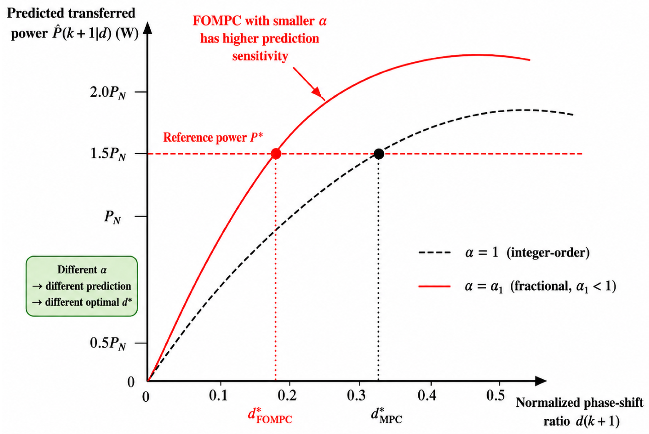
Figure 5 presents representative predicted transferred-power characteristics obtained under a fixed operating point and voltage-history sequence. The variation in the curves reflects the change in the finite-memory weighting distribution. The resulting optimal phase-shift command also depends on the converter operating point and the retained state history.

3.4. Single-Objective Cost Function and Optimal Phase-Shift Solution

The inner-loop objective is to minimize the one-step power-tracking error:

$$J(k,\theta )={\left[\widehat{P}(k+1|\theta )-P^{★}\left(k\right)\right]}^2.$$

(78)

Substituting (75) into (78) gives

$$J(k,\theta )={\left[A_{k}sin\theta +B_k{sin}^2\theta -P^{★}\left(k\right)\right]}^2.$$

(79)

Let

$$z=sin\theta ,0\le z\le 1.$$

(80)

Then,

$$J(k,z)={\left[A_{k}z+B_k{z}^2-P^{★}\left(k\right)\right]}^2.$$

(81)

The unconstrained optimum is obtained by solving

$$B_k{z}^2+A_{k}z-P^{★}\left(k\right)=0.$$

(82)

To avoid numerical division by a small $B_k$, the raw solution is calculated as

$$z_{\mathrm{raw}}^{★}=\left\{\begin{array}{cc}{\displaystyle \frac{-A_k+\sqrt{A_k^2+4B_k{P}^{★}\left(k\right)}}{2B_k}},\hfill & |B_k|>{ϵ}_B,\hfill \\ {\displaystyle \frac{P^{★}\left(k\right)}{A_k}},\hfill & |B_k|\le {ϵ}_B,\hfill \end{array}\right.$$

(83)

where ${ϵ}_B$ is a small positive numerical threshold. The physically feasible solution is

$$z^{★}={sat}_{[0,1]}\left(z_{\mathrm{raw}}^{★}\right).$$

(84)

The optimal phase-shift command and normalized phase-shift ratio are

$${\theta }^{★}(k+1)=arcsin\left(z^{★}\right),$$

(85)

$$d^{★}(k+1)={\displaystyle \frac{{\theta }^{★}(k+1)}{\pi }}.$$

(86)

As shown in Figure 6, the voltage error is first converted into a reference transferred power. The inner loop then determines the phase-shift command analytically using the predictive model and the power-tracking objective.

3.5. Local Small-Signal Stability Analysis

The physical SR-DAB plant is described by the integer-order model

$$C_o{\displaystyle \frac{\mathrm{d}U\left(t\right)}{\mathrm{d}t}}=\mathrm{\Gamma }\left(t\right)sin\theta \left(t\right)-{\displaystyle \frac{U\left(t\right)}{R}}.$$

(87)

Small perturbations around the nominal operating point $(U_0,{\theta }_0,{\mathrm{\Gamma }}_0)$ are defined as

$$U\left(t\right)=U_0+\tilde{U}\left(t\right),$$

(88)

$$\theta \left(t\right)={\theta }_0+\tilde{\theta }\left(t\right),$$

(89)

$$\mathrm{\Gamma }\left(t\right)={\mathrm{\Gamma }}_0+\tilde{\mathrm{\Gamma }}\left(t\right).$$

(90)

Using the first-order approximation

$$sin({\theta }_0+\tilde{\theta })\approx sin{\theta }_0+\tilde{\theta }cos{\theta }_0,$$

(91)

and neglecting second-order terms, the small-signal model is

$$C_o{\displaystyle \frac{\mathrm{d}\tilde{U}\left(t\right)}{\mathrm{d}t}}+{\displaystyle \frac{\tilde{U}\left(t\right)}{R}}={\mathrm{\Gamma }}_{0}cos{\theta }_0\tilde{\theta }\left(t\right)+sin{\theta }_0\tilde{\mathrm{\Gamma }}\left(t\right).$$

(92)

The control-to-output transfer function is

$$G_{u\theta }\left(s\right)={\displaystyle \frac{\tilde{U}\left(s\right)}{\tilde{\theta }\left(s\right)}}={\displaystyle \frac{{\mathrm{\Gamma }}_{0}cos{\theta }_0}{C_{o}s+{\displaystyle \frac{1}{R}}}}.$$

(93)

The source-disturbance-to-output transfer function is

$$G_{u\mathrm{\Gamma }}\left(s\right)={\displaystyle \frac{\tilde{U}\left(s\right)}{\tilde{\mathrm{\Gamma }}\left(s\right)}}={\displaystyle \frac{sin{\theta }_0}{C_{o}s+{\displaystyle \frac{1}{R}}}}.$$

(94)

For the local stability analysis, the inner-loop optimization is linearized around the nominal unsaturated operating point. From (82), the local phase-shift gain is

$$K_{\theta }={\left.{\displaystyle \frac{\partial {\theta }^{★}}{\partial P^{★}}}\right|}_0={\displaystyle \frac{1}{\left(A_0+2B_{0}sin{\theta }_0\right)cos{\theta }_0}}.$$

(95)

The local open-loop transfer function, considering the sampling and computational delay $T_d$, is

$$G_{\mathrm{ol}}\left(s\right)=\left(k_{v1}+{\displaystyle \frac{k_{v2}}{s^{\mu }}}\right)K_{\theta }{e}^{-s{T}_d}{\displaystyle \frac{{\mathrm{\Gamma }}_{0}cos{\theta }_0}{C_{o}s+{\displaystyle \frac{1}{R}}}}.$$

(96)

The local closed-loop transfer function is

$$G_{\mathrm{cl}}\left(s\right)={\displaystyle \frac{G_{\mathrm{ol}}\left(s\right)}{1+G_{\mathrm{ol}}\left(s\right)}}.$$

(97)

Considering source-voltage disturbance, the output-voltage perturbation is

$$\tilde{U}\left(s\right)={\displaystyle \frac{G_{\mathrm{ol}}\left(s\right)}{1+G_{\mathrm{ol}}\left(s\right)}}{\tilde{U}}^{★}\left(s\right)+{\displaystyle \frac{G_{u\mathrm{\Gamma }}\left(s\right)}{1+G_{\mathrm{ol}}\left(s\right)}}\tilde{\mathrm{\Gamma }}\left(s\right).$$

(98)

The resulting local small-signal closed-loop control structure is shown in Figure 7.

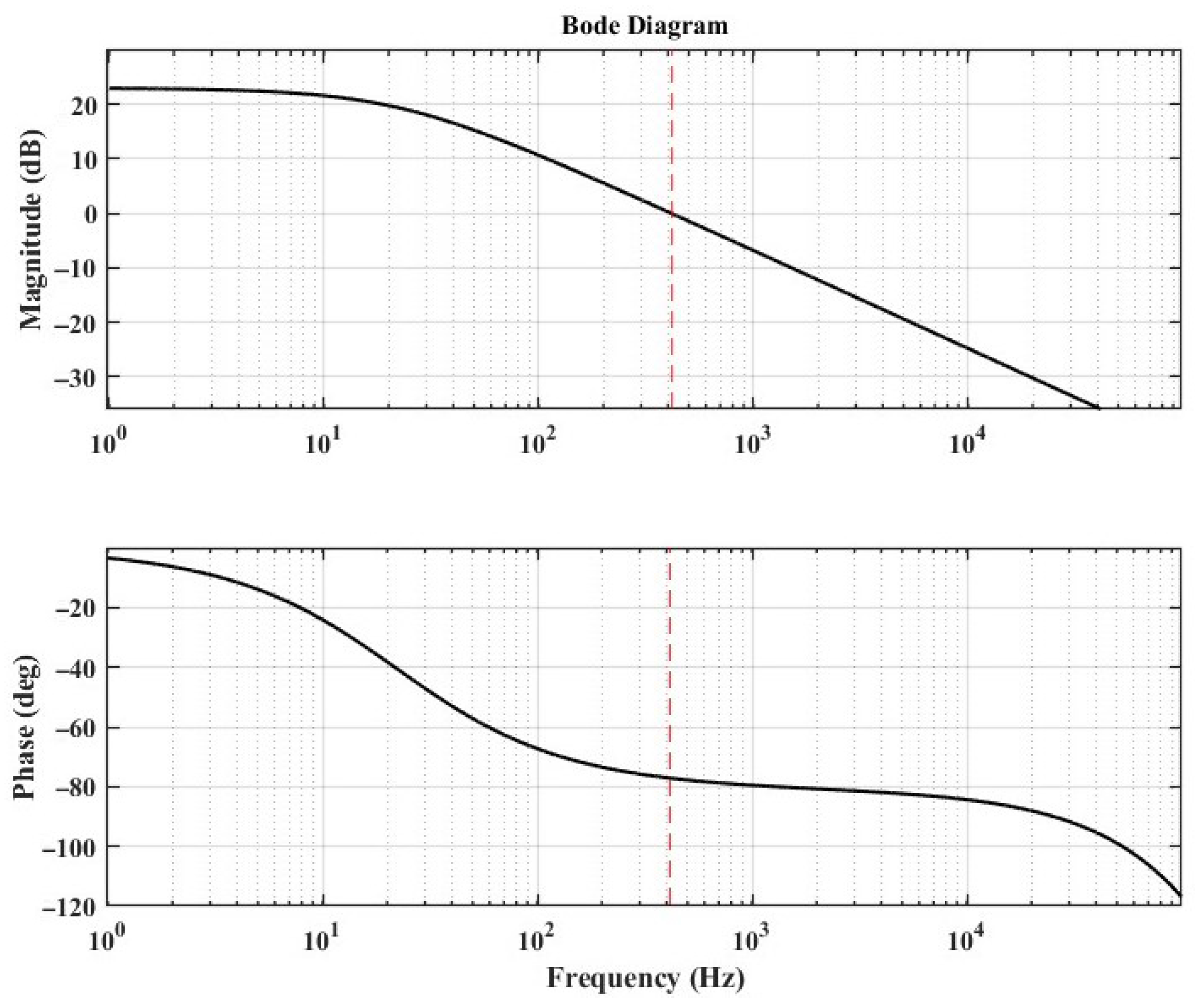
Figure 8 provides a local frequency-domain stability assessment around the nominal operating point.

The power-tracking cost satisfies

$$J(k,\theta )\ge 0,$$

(99)

and the phase-shift command is constrained by

$$0\le d^{★}(k+1)\le 0.5.$$

(100)

Since $J(k,\theta )$ is continuous with respect to $\theta$ and the admissible set $[0,\pi /2]$ is compact, the Weierstrass theorem guarantees the existence of at least one minimizer for the constrained scalar optimization problem. The closed-loop behavior under plant-model mismatch is examined in Section 4.3.

3.6. GWO-Based Parameter Tuning

The FOPI outer-loop parameters $k_{v1}$, $k_{v2}$, and $\mu$, together with the fractional-order parameter $\alpha$ of the predictive inner loop, determine the transient response and steady-state performance of the proposed controller. The parameter vector is defined as

$$\mathrm{\Theta }={\left[k_{v1},k_{v2},\mu ,\alpha \right]}^{\mathrm{T}}.$$

(101)

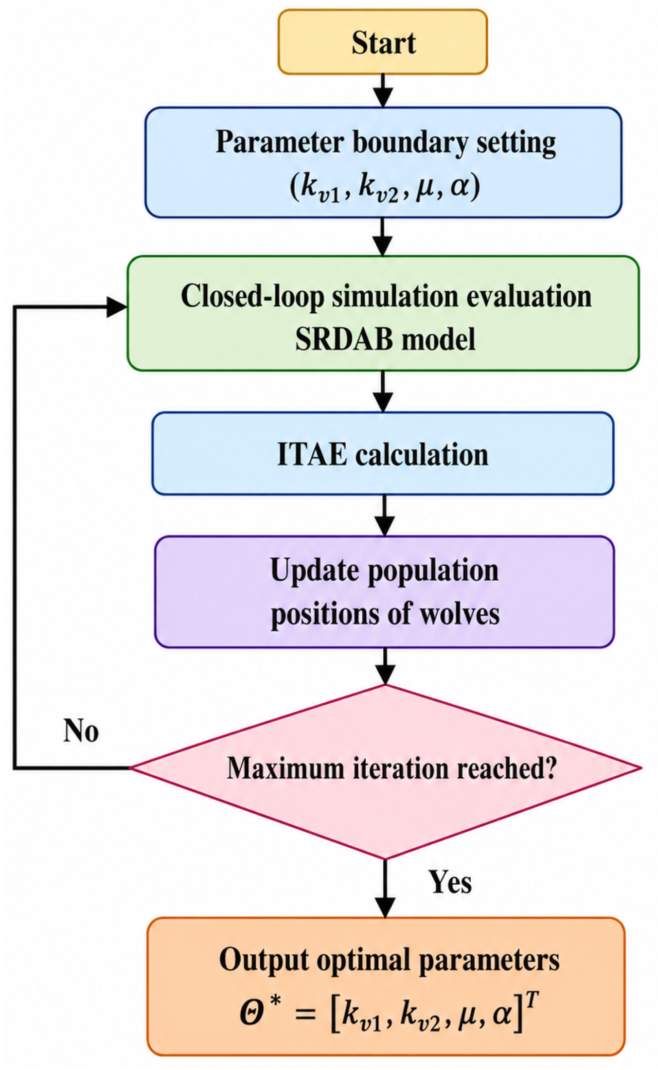
The GWO algorithm is employed to coordinate the selection of these parameters before real-time controller execution. Each candidate parameter vector is evaluated using the same converter model under representative input-voltage disturbances, load variations, and output-voltage reference changes. The integral of time-weighted absolute error is adopted as the fitness function:

$$J_{\mathrm{ITAE}}={\int }_0^{T_{\mathrm{obs}}}t\left|U^{★}\left(t\right)-U\left(t\right)\right|\mathrm{d}t,$$

(102)

where $T_{\mathrm{obs}}$ denotes the observation interval. For digital evaluation, (102) is expressed as

$$J_{\mathrm{ITAE}}={\displaystyle \sum _{k=0}^N}k{T}_s\left|U^{★}\left(k\right)-U\left(k\right)\right|,$$

(103)

where $T_s$ is the sampling interval used for fitness evaluation and N is the number of samples within $T_{\mathrm{obs}}$. The tuning objective is

$${\mathrm{\Theta }}^{★}=arg\underset{\mathrm{\Theta }}{min}{J}_{\mathrm{ITAE}}.$$

(104)

The considered tuning problem is evaluated through a nonlinear converter simulation, and an explicit analytical gradient of the ITAE objective function is not readily available. A derivative-free optimization method is therefore adopted. GWO is selected because its search process does not require numerical gradient evaluation and involves no crossover or mutation operations. In comparison with gradient-based tuning, it avoids repeated perturbation-based gradient calculations, whereas its position-update mechanism requires fewer algorithm-specific operators than a conventional genetic algorithm. In this study, GWO is used for coordinated offline parameter selection rather than online optimization.

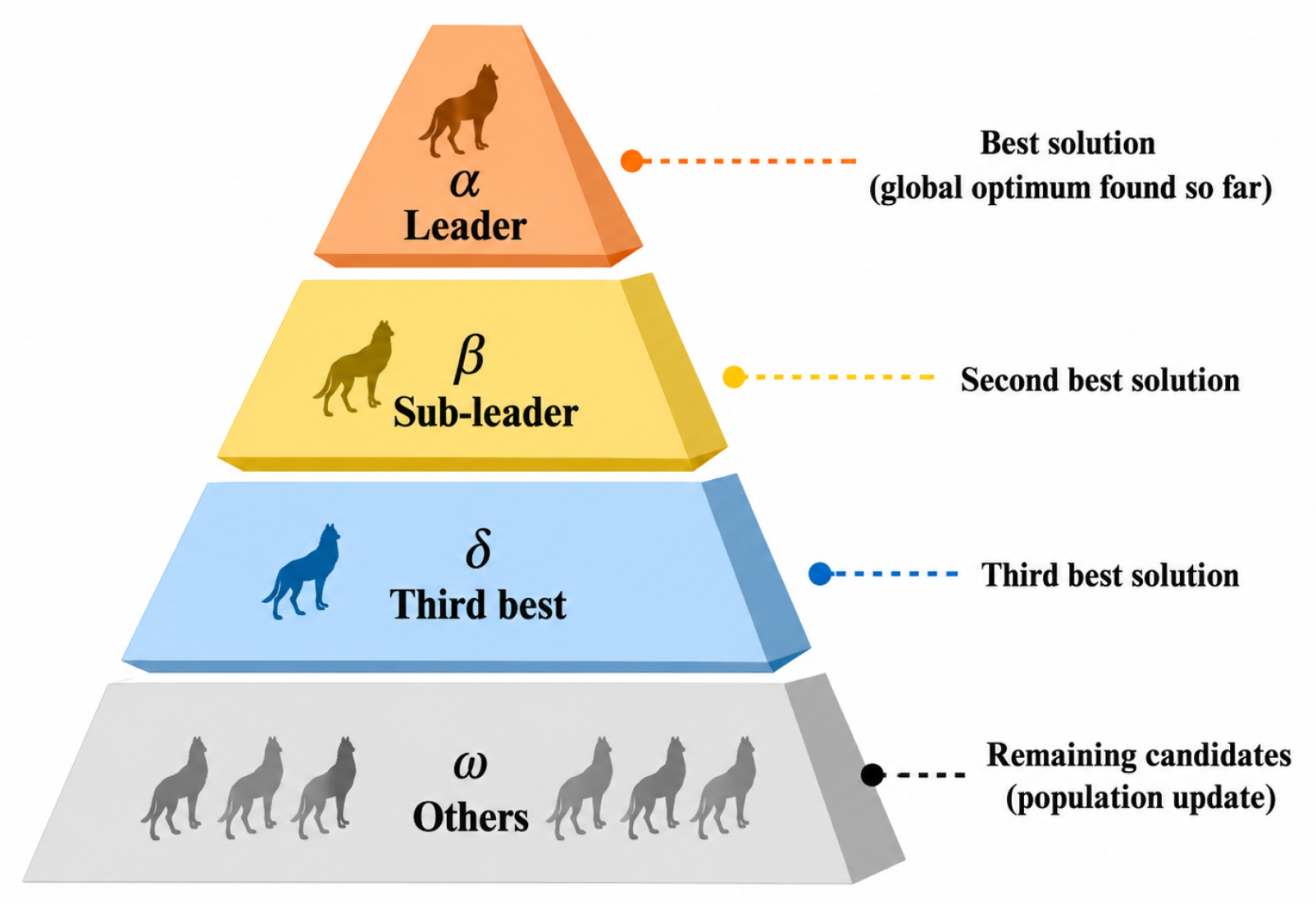
In the GWO framework, each gray wolf represents one candidate parameter vector. The best three candidates are denoted as the $\alpha$-, $\beta$-, and $\delta$-wolves. These symbols indicate the hierarchy of the optimizer and are distinct from the fractional-order parameter $\alpha$ in (101). Let $\mathbf{X}$ denote the current search position. The distance vectors with respect to the three leading wolves are

$${\mathbf{D}}_{\alpha }=\left|{\mathbf{C}}_1{\mathbf{X}}_{\alpha }-\mathbf{X}\right|,$$

(105)

$${\mathbf{D}}_{\beta }=\left|{\mathbf{C}}_2{\mathbf{X}}_{\beta }-\mathbf{X}\right|,$$

(106)

$${\mathbf{D}}_{\delta }=\left|{\mathbf{C}}_3{\mathbf{X}}_{\delta }-\mathbf{X}\right|.$$

(107)

The three guided candidate positions are obtained as

$${\mathbf{X}}_1={\mathbf{X}}_{\alpha }-{\mathbf{A}}_1{\mathbf{D}}_{\alpha },{\mathbf{X}}_2={\mathbf{X}}_{\beta }-{\mathbf{A}}_2{\mathbf{D}}_{\beta },{\mathbf{X}}_3={\mathbf{X}}_{\delta }-{\mathbf{A}}_3{\mathbf{D}}_{\delta }.$$

(108)

The search position for the next generation is updated according to

$$\mathbf{X}(\ell +1)={\displaystyle \frac{{\mathbf{X}}_1+{\mathbf{X}}_2+{\mathbf{X}}_3}{3}}.$$

(109)

The coefficient vectors are defined as

$${\mathbf{A}}_i=2a{\mathbf{r}}_{1i}-a,{\mathbf{C}}_i=2{\mathbf{r}}_{2i},i=1,2,3,$$

(110)

where ${\mathbf{r}}_{1i}$ and ${\mathbf{r}}_{2i}$ are uniformly distributed random vectors in $[0,1]$. The convergence factor is updated as

$$a=2-{\displaystyle \frac{2\ell }{N_{max}}},$$

(111)

where ℓ denotes the current generation and $N_{max}$ is the maximum number of generations.

The optimizer hierarchy and the offline parameter-tuning procedure are illustrated in Figure 9 and Figure 10, respectively.

The offline search employs a population of $N_p=20$ candidate solutions and a maximum of $N_{max}=100$ generations. Since the initial population is evaluated before the iterative position updates, the maximum number of objective-function evaluations for one optimization run is

$$N_{\mathrm{eval}}=N_p\left(N_{max}+1\right)=20\times 101=2020.$$

(112)

After convergence, the tuned parameter vector is expressed as

$${\mathrm{\Theta }}^{★}={\left[k_{v1}^{★},k_{v2}^{★},{\mu }^{★},{\alpha }^{★}\right]}^{\mathrm{T}}.$$

(113)

For the operating range considered in this study, the offline optimization gives

$${\mathrm{\Theta }}^{★}={\left[28,1200,0.86,0.75\right]}^{\mathrm{T}}.$$

(114)

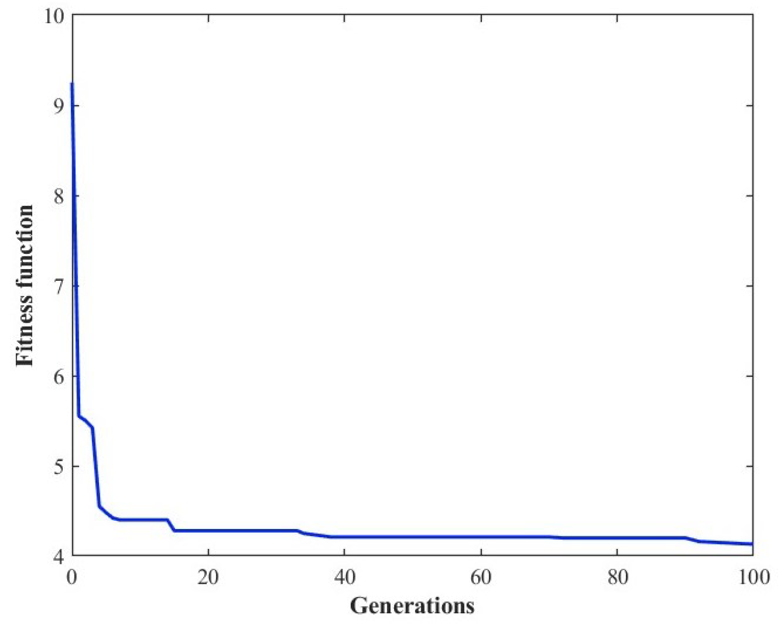
As shown in Figure 11, the best ITAE value decreases rapidly during the initial generations and subsequently approaches a stable value. Convergence is identified as the generation at which the best fitness value enters and remains within the final 1% fitness interval. Based on this criterion, the optimization converges after approximately 61 generations. One complete optimization run requires approximately 1122 s on a computer equipped with an Intel Core i9-12900H processor and 32 GB of RAM using MATLAB/Simulink R2024a. The configuration and computational cost of the offline parameter-tuning process are summarized in

Table 2. Configuration and computational cost of the offline GWO parameter-tuning procedure.

Item	Value
Number of decision variables	4
Population size $N_p$	20
Maximum generations $N_{max}$	100
Convergence generation $N_{\mathrm{conv}}$	61
Objective-function evaluations $N_{\mathrm{eval}}$	2020
Offline computation time	1122 s
Computing processor	Intel Core i9-12900H
Computer memory	32 GB
Software platform	MATLAB/Simulink R2024a
Optimized parameter vector	${[28,1200,0.86,0.75]}^{\mathrm{T}}$

.

The optimized parameter set is fixed in the FOPI outer loop and the fractional-order predictive inner loop during converter operation. Therefore, the population update, candidate evaluation, and iterative search processes are not executed by the real-time digital controller. The resulting controller parameters and finite-memory settings are summarized in

Table 3. Controller parameters and finite-memory settings.

Parameter	Value
Outer-loop proportional gain $k_{v1}$	28
Outer-loop fractional-integral gain $k_{v2}$	1200
Outer-loop fractional order $\mu$	0.86
Inner-loop fractional order $\alpha$	0.75
Inner-loop sampling period $T_c$	10 $\mathsf{\mu }$s
Outer-loop sampling period $T_v$	100 $\mathsf{\mu }$s
Inner-loop memory length $N_c$	20
Outer-loop memory length $N_v$	100
Inner-loop memory window $N_c{T}_c$	0.20 ms
Outer-loop memory window $N_v{T}_v$	10 ms
GWO execution mode	Offline parameter tuning

.

The Grünwald–Letnikov coefficients are precomputed and stored together with the controller constants. Each inner-loop update evaluates a 20-term weighted accumulation, whereas the 101-term outer-loop convolution is evaluated once every ten inner-loop intervals. Consequently, the finite-memory calculation requires approximately 20 multiply–accumulate operations during a regular inner-loop interval and 121 multiply–accumulate operations when the inner- and outer-loop updates coincide. The corresponding average operation count is

$${\overline{N}}_{\mathrm{MAC}}={\displaystyle \frac{9\times 20+121}{10}}=30.1$$

(115)

multiply–accumulate operations per $10\mathsf{\mu }\mathrm{s}$ inner-loop interval. The two state-history buffers and their single-precision weighting coefficients require approximately

$$M_{\mathrm{hist}}=2(N_c+N_v+1)\times 4=2(20+100+1)\times 4=968\mathrm{bytes},$$

(116)

which is approximately 1.0 kB. These operation and storage estimates describe the finite-memory controller implementation and exclude the offline GWO parameter-search process.

4. Simulation Validation for Energy Mutual Assistance of Field Medical Electric Vehicles

4.1. Simulation Platform and Operating Conditions

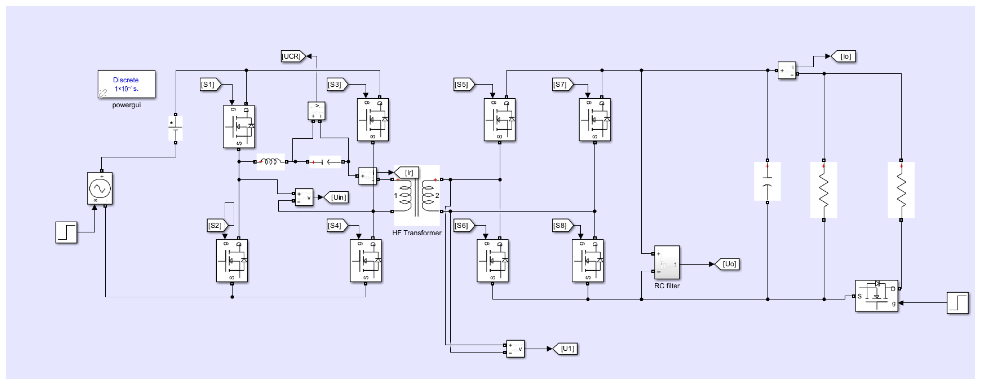
To verify the effectiveness of the proposed control strategy in the energy mutual-assistance scenario of field medical electric vehicles, an SRDAB simulation platform was established in MATLAB/Simulink, as shown in Figure 12. In this platform, the input side represents the donor vehicle, while the output side represents the vehicle that receives energy. The power stage adopts single-phase-shift modulation. The control stage employs the proposed dual-loop structure, in which the GWO-optimized fractional-order proportional–integral outer loop generates the reference transferred power and the fractional-order predictive inner loop calculates the optimal phase-shift command online.

The nominal operating condition was selected as an input voltage of 100 V, an output-voltage reference of 250 V, and a load resistance of 25 $\mathrm{\Omega }$. Under this condition, the nominal output current is 10 A and the nominal output power is 2.50 kW. The switching frequency and the resonant frequency were set to 100 kHz and 80 kHz, respectively.

To evaluate dynamic performance under successive operating-conditions transitions, the input voltage was changed from 100 V to 90 V and then to 120 V. Subsequently, the load resistance changed from 25 $\mathrm{\Omega }$ to 50 $\mathrm{\Omega }$ and then to 22 $\mathrm{\Omega }$. Finally, the output-voltage reference was changed from 250 V to 240 V and then to 260 V.

For a consistent comparison, all five controllers used the same switching-level SRDAB plant, disturbance sequence, phase-shift limits, measured signals, and controller-update periods. The inner and outer loops were updated at $T_c=10\mathsf{\mu }$s and $T_v=100\mathsf{\mu }$s, respectively. The IOMPC benchmark consists of a conventional PI power-reference outer loop and an integer-order continuous-control-set MPC phase-shift inner loop. FOMPC retains the same dual-loop arrangement but introduces fractional orders selected by manual tuning. GWO-IOMPC fixes the two fractional orders at unity and uses GWO only to tune the outer-loop gains, whereas GWO-FOMPC jointly tunes the outer-loop gains and the two fractional orders. STSMC is included as a nonlinear-control benchmark. The controller parameters used to generate Figure 13, Figure 14, Figure 15, Figure 16 and Figure 17 are summarized in

Table 4. Controller parameters used in the comparative simulations.

Controller	${\mathit{k}}_{\mathit{v}1}$	${\mathit{k}}_{\mathit{v}2}$	$\mathit{\mu }$	$\mathit{\alpha }$	Finite-Memory Setting	Parameter Selection
IOMPC	650	8000	1	1	Not used	Manual tuning
FOMPC	650	8000	0.85	0.90	$N_v=100$, $N_c=20$	Manual tuning
STSMC	$k_1=500$, $k_2=5000$, $\varphi =0.20$				Not used	Manual tuning
GWO-IOMPC	28	1200	1	1	Not used	Offline GWO
GWO-FOMPC	28	1200	0.86	0.75	$N_v=100$, $N_c=20$	Offline GWO

. The main simulation parameters and operating conditions are listed in

Table 5. SRDAB model parameters and nominal operating conditions used in simulation.

Parameter	Value
Nominal input voltage $V_{\mathrm{in},\mathrm{nom}}$	100 V
Nominal output-voltage reference $V_{\mathrm{o},\mathrm{nom}}^{*}$	250 V
Nominal load resistance $R_{\mathrm{L},\mathrm{nom}}$	25 $\mathrm{\Omega }$
Nominal output current $I_{\mathrm{o},\mathrm{nom}}$	10 A
Nominal output power $P_{\mathrm{o},\mathrm{nom}}$	2.50 kW
Transformer turns ratio n	1:1
Switching frequency $f_{\mathrm{s}}$	100 kHz
Resonant frequency $f_{\mathrm{r}}$	80 kHz
Resonant inductance $L_{\mathrm{r}}$	20 $\mathsf{\mu }$H
Resonant capacitance $C_{\mathrm{r}}$	200 nF
Input-side capacitor $C_{\mathrm{in}}$	470 $\mathsf{\mu }$F
Output-side capacitor $C_{\mathrm{o}}$	470 $\mathsf{\mu }$F

.

Here, $k_{v1}$ and $k_{v2}$ denote the proportional and integral or fractional-integral gains of the voltage-regulation outer loop. The STSMC gains are method-specific and are therefore not interpreted as direct counterparts of $k_{v1}$ and $k_{v2}$. For the two fractional-order controllers, the retained memory windows are $N_v{T}_v=10$ ms and $N_c{T}_c=0.20$ ms.

4.2. Comprehensive Dynamic Simulation Comparison Under Multiple Operating Conditions

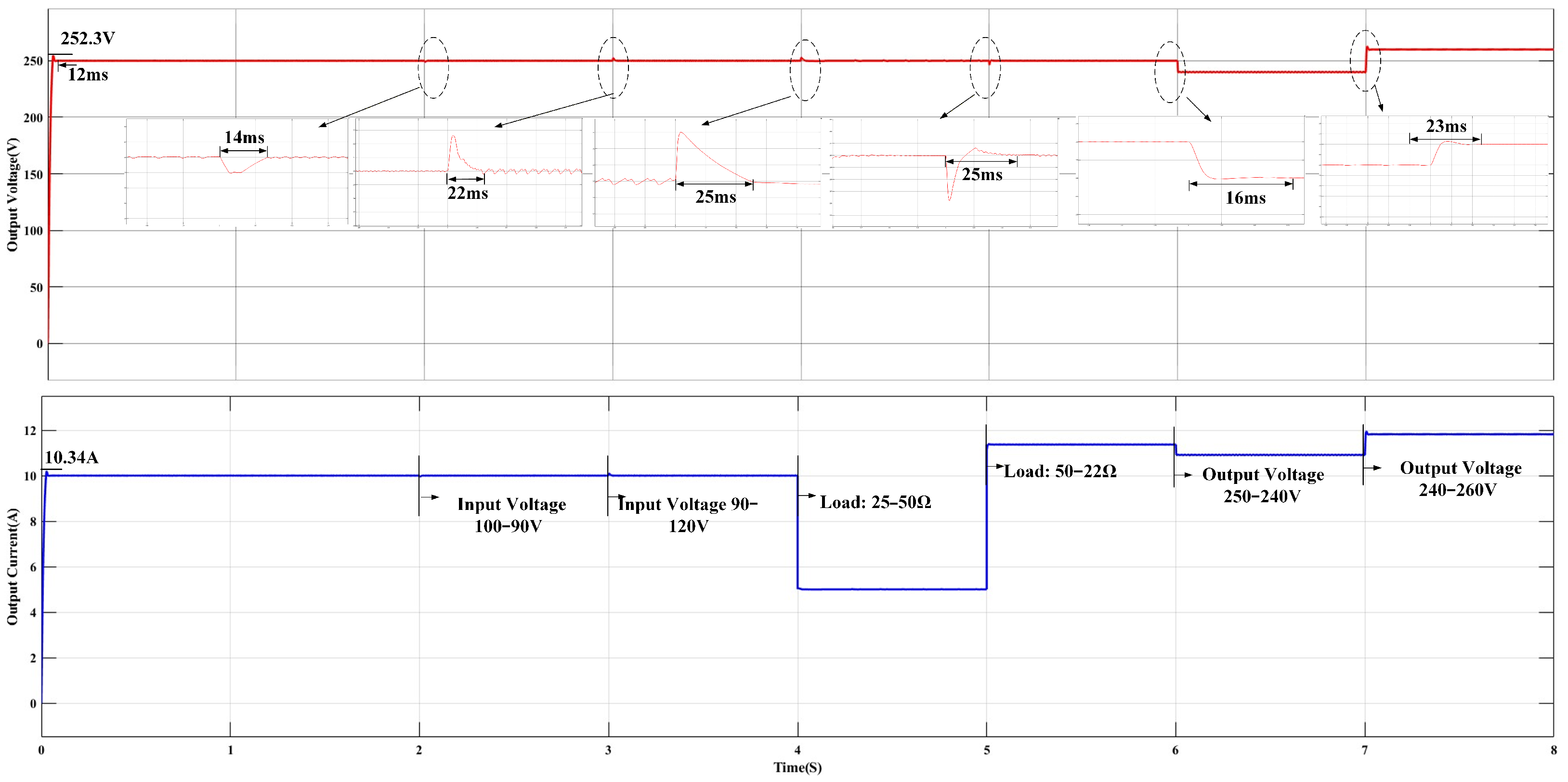
A sequence of operating-condition transitions was applied to the SRDAB converter to comprehensively evaluate the dynamic performance of the proposed GWO-FOMPC strategy. The initial operating condition was set as $V_{\mathrm{in}}=100$ V, $V_{\mathrm{o}}^{*}=250$ V, and $R_{\mathrm{L}}=25\mathrm{\Omega }$.

At $t=2$ s, the input voltage was changed from 100 V to 90 V. At $t=3$ s, the input voltage was changed from 90 V to 120 V. At $t=4$ s, the load resistance was changed from 25 $\mathrm{\Omega }$ to 50 $\mathrm{\Omega }$. At $t=5$ s, the load resistance was changed from 50 $\mathrm{\Omega }$ to 22 $\mathrm{\Omega }$. At $t=6$ s, the output-voltage reference was reduced from 250 V to 240 V. At $t=7$ s, the output-voltage reference was increased from 240 V to 260 V.

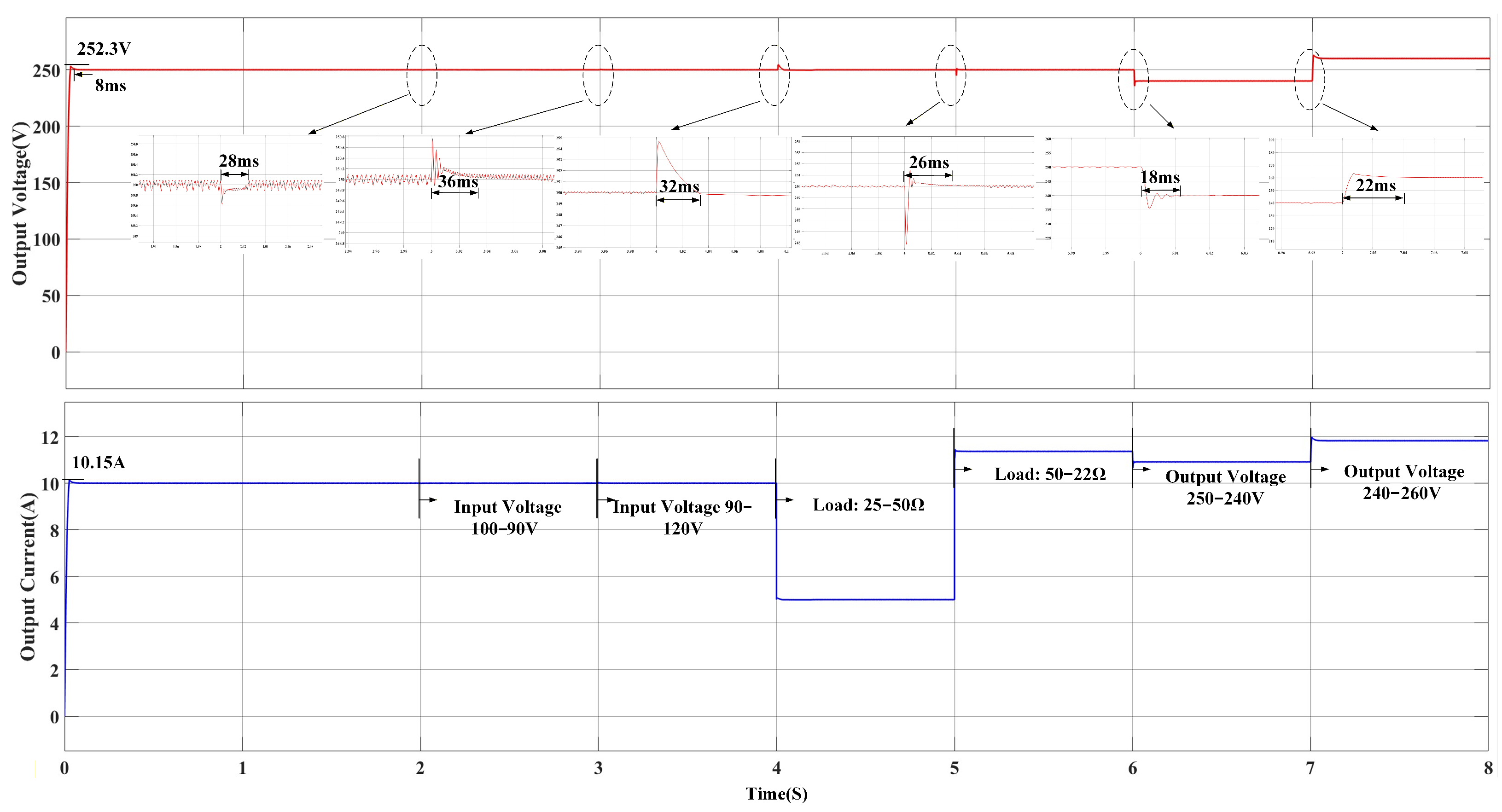
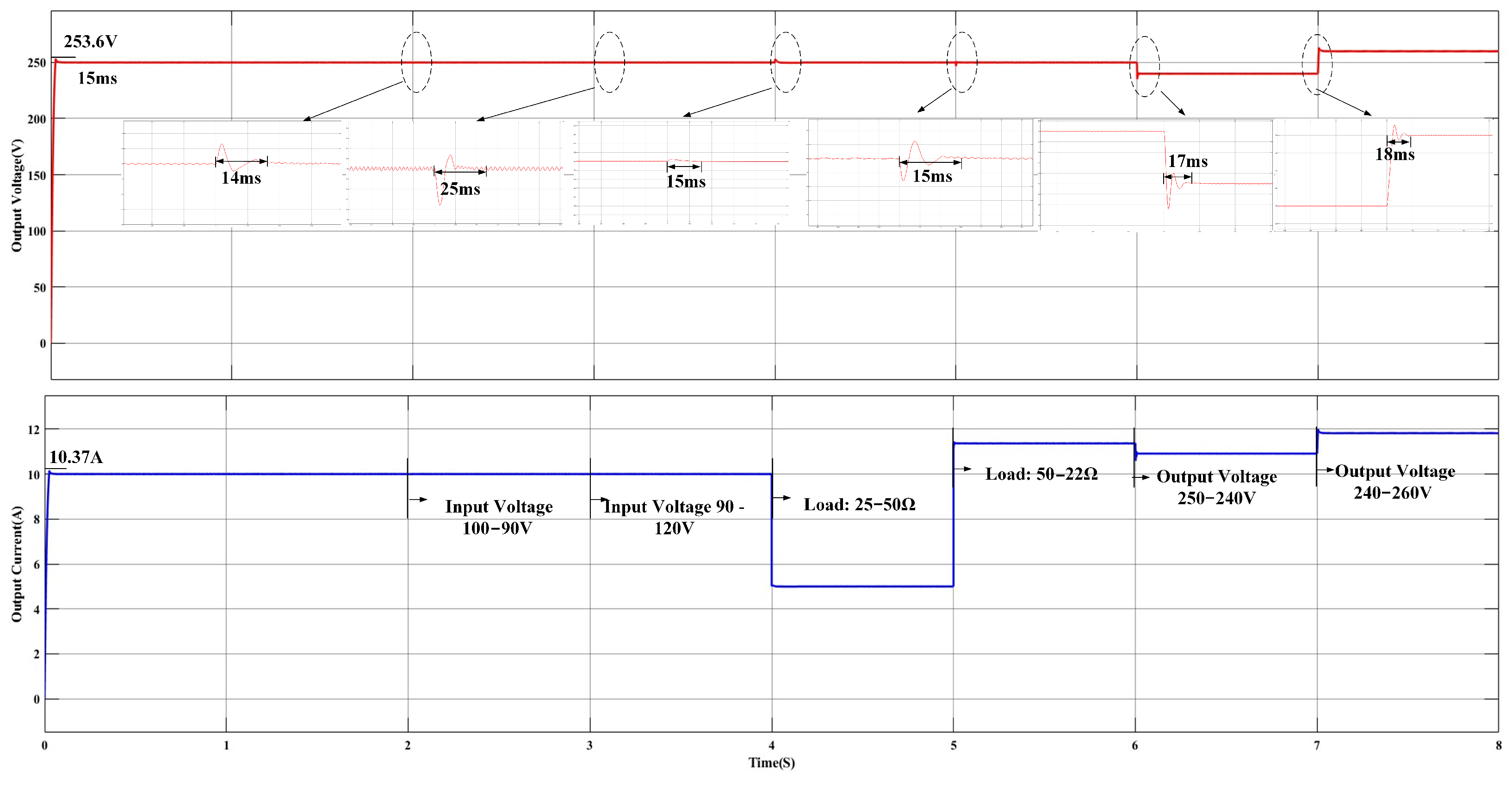
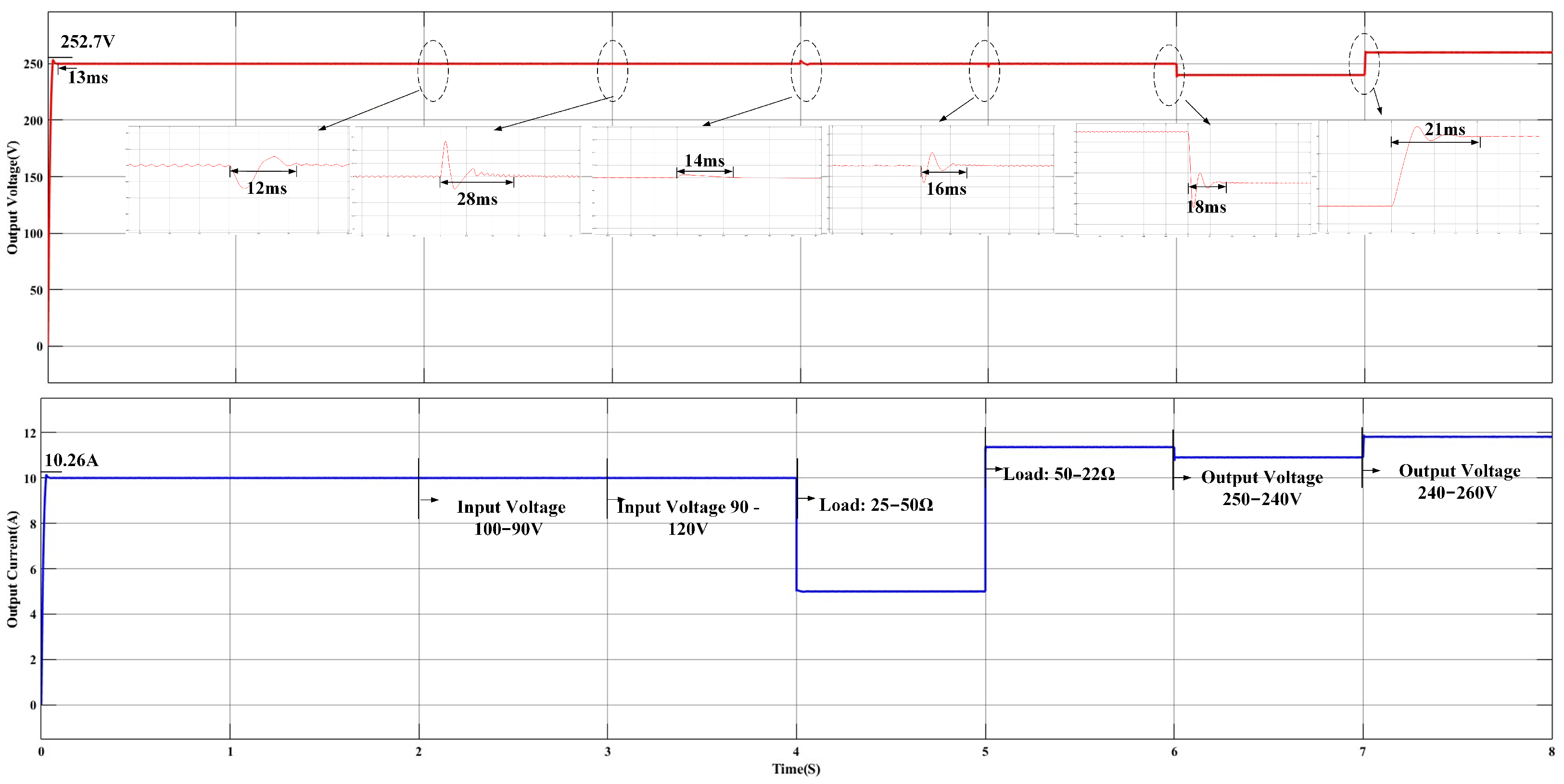
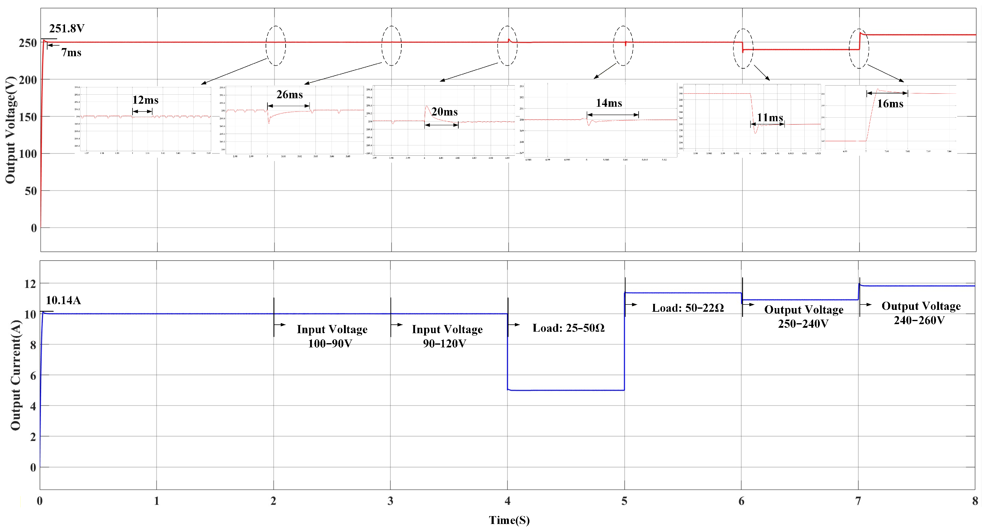
The output-voltage and output-current responses of IOMPC, FOMPC, STSMC, GWO-IOMPC, and GWO-FOMPC are shown in Figure 13, Figure 14, Figure 15, Figure 16 and Figure 17. The settling time is measured from the instant at which the operating condition changes until the output voltage enters and remains within a $\pm 2\%$ band around its final reference. The resulting settling times are summarized in

Table 6. Output-voltage settling times under the successive simulation transitions.

Controller	$\mathit{t}=2$ s	$\mathit{t}=3$ s	$\mathit{t}=4$ s	$\mathit{t}=5$ s	$\mathit{t}=6$ s	$\mathit{t}=7$ s	Mean	Maximum
			Settling Time (ms)
IOMPC	28	36	32	26	18	22	27.0	36
FOMPC	12	26	20	14	11	16	16.5	26
STSMC	9	20	55	10	7	11	18.7	55
GWO-IOMPC	14	22	25	25	16	23	20.8	25
GWO-FOMPC	11	17	12	11	14	18	13.8	18

. This common definition is applied to all controllers and all six transitions.

All five controllers maintain bounded output-voltage regulation over the investigated sequence, but their transient characteristics differ. Fractional-order augmentation alone reduces the mean settling time from 27.0 ms for IOMPC to 16.5 ms for FOMPC. Offline optimization of the integer-order controller reduces the mean value to 20.8 ms for GWO-IOMPC. The proposed GWO-FOMPC gives the lowest mean settling time of 13.8 ms and the lowest worst-case settling time of 18 ms. Relative to IOMPC, FOMPC, STSMC, and GWO-IOMPC, its mean settling time is reduced by approximately 48.8%, 16.2%, 25.9%, and 33.6%, respectively.

The results also show that no single controller is the fastest at every individual transition. STSMC gives shorter settling times at $t=2$, 5, 6, and 7 s, but its response increases to 55 ms for the load reduction at $t=4$ s. FOMPC is slightly faster than GWO-FOMPC during the two reference-voltage transitions. Consequently, the principal advantage observed for GWO-FOMPC is its lower aggregate and worst-case settling time over the complete operating sequence, rather than pointwise superiority under every transition. The comparison between IOMPC and GWO-IOMPC isolates the effect of offline gain optimization, whereas the comparison between GWO-IOMPC and GWO-FOMPC indicates the additional contribution of the finite-memory fractional-order predictor.

4.3. Robustness Under Physical-Parameter Mismatch

The closed-loop response to physical-parameter mismatch was examined by varying the parameters of the switching-level SRDAB plant while retaining the nominal model in the predictor. The nominal operating point was $V_{\mathrm{in}}=100\mathrm{V}$, $V_{\mathrm{o}}^{*}=250\mathrm{V}$, and $R_{\mathrm{L}}=25\mathrm{\Omega }$. Individual deviations of $\pm 10\%$ were applied to $L_r$ and $C_r$, and deviations of $\pm 20\%$ were applied to $C_o$. A combined case with $L_r=1.1L_{r,\mathrm{nom}}$, $C_r=1.1C_{r,\mathrm{nom}}$, and $C_o=1.2C_{o,\mathrm{nom}}$ was also considered. In all cases, the controller used $L_{r,\mathrm{nom}}=20\mathsf{\mu }\mathrm{H}$, $C_{r,\mathrm{nom}}=200\mathrm{nF}$, and $C_{o,\mathrm{nom}}=470\mathsf{\mu }\mathrm{F}$. An input-voltage step from 100 V to 90 V was applied after the initial steady state to compare the transient voltage regulation and one-step prediction accuracy under the same disturbance.

The one-step voltage-prediction error is defined as

$$e_{\mathrm{pred}}\left(k\right)=U\left(k\right)-\widehat{U}\left(k\right|k-1),$$

(117)

and its root-mean-square value over an observation interval of N samples is

$${\mathrm{RMSE}}_{\mathrm{pred}}=\sqrt{{\displaystyle \frac{1}{N}}{\displaystyle \sum _{k=1}^N}{e}_{\mathrm{pred}}^2\left(k\right)}.$$

(118)

The settling time is evaluated using a $\pm 2\%$ band around the 250 V reference. The maximum voltage deviation, settling time, prediction RMSE, and peak resonant current obtained from the switching-level simulations are summarized in

Table 7. Switching-level simulation results under physical-parameter mismatch.

Plant Condition	${\left|\mathbf{\Delta }\mathit{U}\right|}_{max}$ (V)	${\mathit{t}}_{\mathit{s}}$ (ms)	${\mathbf{RMSE}}_{\mathbf{pred}}$ (V)	${\mathit{I}}_{\mathit{r},\mathbf{pk}}$ (A)
Nominal parameters	3.5	12.2	0.018	56.0
$L_r+10\%$	6.3	17.8	0.062	49.0
$L_r-10\%$	7.8	20.3	0.094	72.0
$C_r+10\%$	5.2	15.9	0.044	52.0
$C_r-10\%$	6.9	18.5	0.071	64.0
$C_o+20\%$	3.1	16.3	0.026	55.0
$C_o-20\%$	6.2	16.8	0.036	60.0
Combined mismatch	9.7	25.7	0.083	49.0

.

The nominal model gives a maximum voltage deviation of 3.5 V and a prediction RMSE of 0.018 V. Decreasing $L_r$ by 10% produces the largest individual-case prediction RMSE and resonant-current peak. This trend is consistent with (41): a reduction in $L_r$ decreases $X_r$ and increases the magnitude of the phase-shift-to-power coefficient. Variations in $C_r$ cause the same directional change but with a smaller local sensitivity. Increasing $C_o$ reduces the maximum voltage deviation while extending the settling process, whereas decreasing $C_o$ increases the voltage excursion because the same instantaneous power imbalance produces a larger voltage slew rate. Under the combined mismatch, the output voltage returns to the specified regulation band within 25.7 ms, although the maximum deviation and prediction error are larger than in the nominal case. The results therefore show bounded closed-loop regulation over the investigated parameter range and provide the numerical counterpart to the coefficient sensitivities derived in Section 2.6.

5. Hardware Prototype Validation for Energy Mutual Assistance of Field Medical Electric Vehicles

5.1. Hardware Prototype and Test Platform

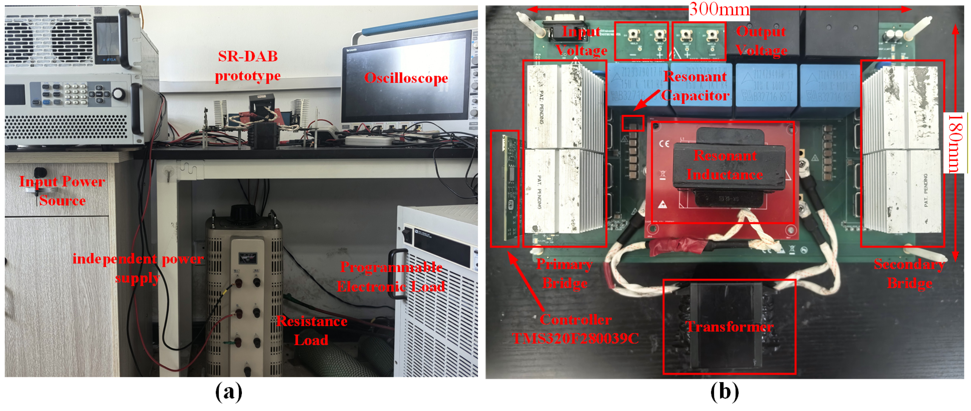
To verify the converter-level implementation and dynamic behavior of the proposed control strategy, an SRDAB hardware prototype and experimental test platform were established, as shown in Figure 18. The experimental platform consists of a programmable dc source, an auxiliary power supply, a digital oscilloscope, the SRDAB prototype, and a programmable electronic load. The programmable source and electronic load emulate the dc-terminal behavior of the donor and recipient sides, respectively; they do not reproduce the electrochemical dynamics, battery-management constraints, or communication functions of complete EV battery systems.

The SRDAB prototype adopts single-phase-shift modulation and operates at a fixed switching frequency of 100 kHz. Isolated dc power transfer is achieved by regulating the phase-shift angle between the primary- and secondary-side full bridges. A TI TMS320F280039C digital controller performs signal acquisition, reference-power generation, finite-memory prediction, analytical phase-shift calculation, and PWM updating. The GWO procedure is executed only during the offline controller-design stage, and the optimized parameter vector is fixed during real-time operation. The main hardware and digital-control parameters are summarized in

Table 8. Main components and experimental platform of the SRDAB prototype.

Category	Parameter	Value
Operating conditions	Nominal input voltage $V_{\mathrm{in}}$	100 V
	Nominal output-voltage reference $V_{\mathrm{o}}^{*}$	250 V
	Output-voltage range investigated experimentally	240–260 V
	Load-resistance range investigated experimentally	22–50 $\mathrm{\Omega }$
	Nominal operating point	250 V, 10 A, 2.50 kW
	Maximum output power investigated dynamically	2.84 kW
Main components	Primary-side MOSFETs	Infineon IMZA120R030M1H
	Secondary-side MOSFETs	Infineon IMW120R014M1H
	High-frequency transformer core	EE65
	Digital controller	TI TMS320F280039C

, while the dynamic and efficiency-test conditions are listed in

Table 9. Operating-condition sequences used in the hardware experiments.

Test Sequence	Input Voltage ${\mathit{V}}_{\mathbf{in}}$	Output-Voltage Reference ${\mathit{V}}_{\mathit{o}}^{*}$	Load Resistance ${\mathit{R}}_{\mathit{L}}$	Corresponding Output Power ${\mathit{P}}_{\mathit{o}}$
Input-voltage steps	$100\to 110\to 100$ V	250 V	25 $\mathrm{\Omega }$	2.50 kW
Reference-voltage steps	100 V	$250\to 240\to 260$ V	25 $\mathrm{\Omega }$	$2.50\to 2.304\to 2.704$ kW
Load-resistance steps	100 V	250 V	$25\to 50\to 22$ $\mathrm{\Omega }$	$2.50\to 1.25\to 2.84$ kW
Efficiency measurement	100 V	250 V	Variable electronic load	$0.5$–$2.5$ kW

.

The 2.50 kW value denotes the nominal operating point rather than the maximum power investigated in the dynamic experiments. As shown in Table 9, the load-step experiment covers 1.25–2.84 kW and uses the same $25\to 50\to 22\mathrm{\Omega }$ resistance sequence as the comparative simulations. This correspondence allows the load-transient responses obtained in simulation and experiment to be compared under consistent steady-state operating points.

5.2. Dynamic Performance Comparison Under Input-Voltage Steps

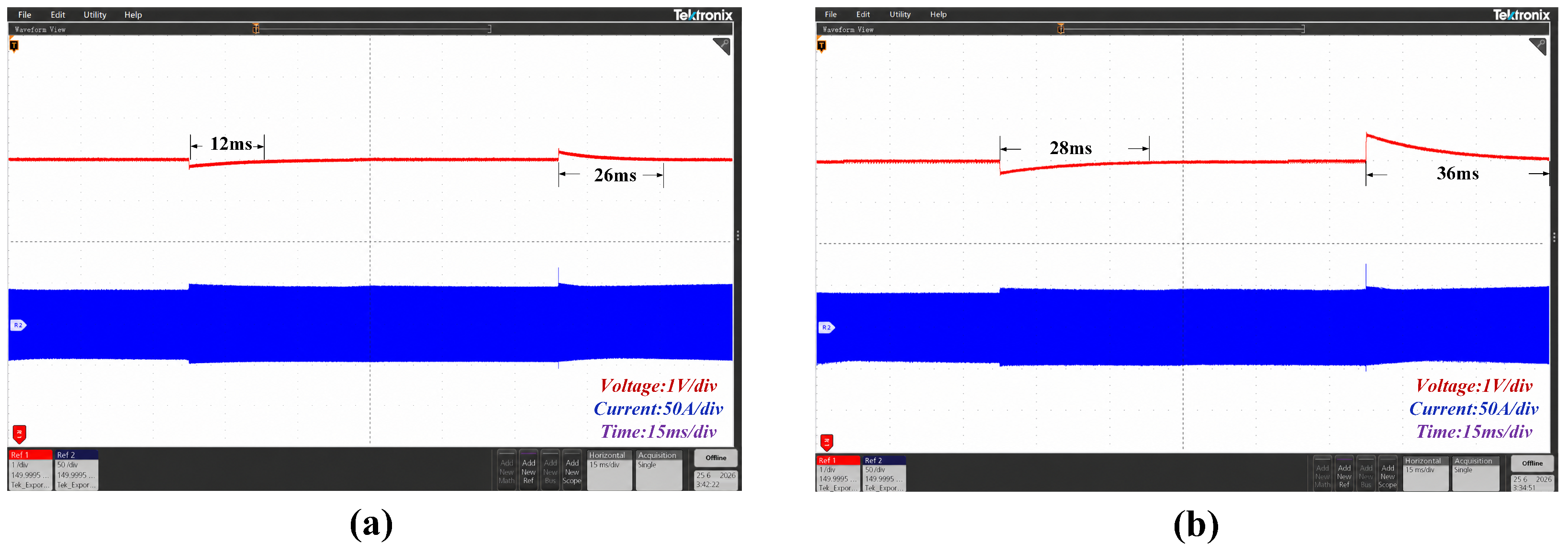
To evaluate disturbance rejection under source-voltage variation, the input voltage was increased from 100 V to 110 V at $t=t_1$ and restored to 100 V at $t=t_2$, while $V_o^{*}=250$ V and $R_L=25\mathrm{\Omega }$ were maintained. The corresponding experimental waveforms are shown in Figure 19, where panels (a) and (b) correspond to GWO-FOMPC and IOMPC, respectively. As in the simulations, the settling time is determined using a $\pm 2\%$ band around the final output-voltage reference.

Both controllers restore the output voltage after the two source-voltage transitions. GWO-FOMPC gives settling times of approximately 12 ms and 26 ms, whereas IOMPC requires approximately 28 ms and 36 ms. The corresponding reductions are 57.1% and 27.8%. The resonant-current disturbance remains transient in both cases, and no sustained oscillation is observed after the output voltage returns to its regulation band. These measurements support improved converter-level rejection of the emulated donor-side voltage variation.

5.3. Dynamic Performance Comparison Under Output-Voltage Reference Steps

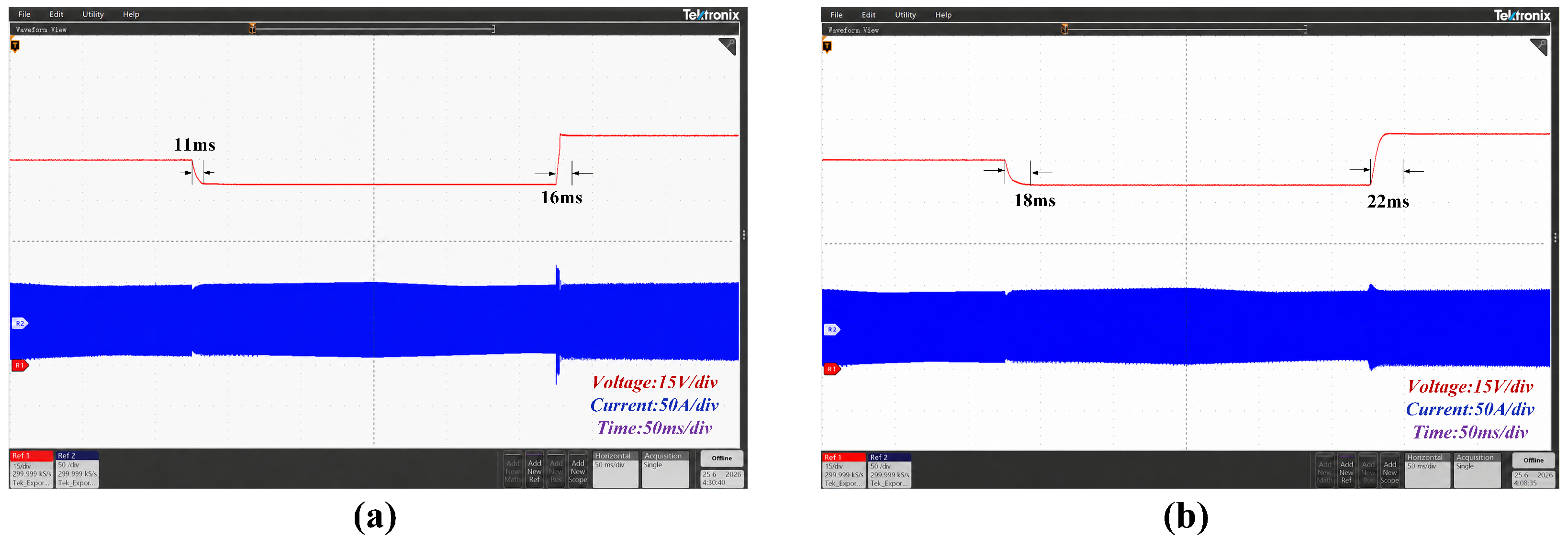
To verify reference-tracking performance, the input voltage and load resistance were fixed at 100 V and 25 $\mathrm{\Omega }$, respectively. The output-voltage reference was changed from 250 V to 240 V at $t=t_1$ and then from 240 V to 260 V at $t=t_2$. The corresponding experimental waveforms are shown in Figure 20, where panels (a) and (b) correspond to GWO-FOMPC and IOMPC, respectively.

Both controllers track the new voltage commands without sustained oscillation. The downward and upward transitions settle in approximately 11 ms and 16 ms under GWO-FOMPC, compared with 18 ms and 22 ms under IOMPC. These values correspond to reductions of 38.9% and 27.3%, respectively. The result confirms that the fractional-order dual-loop controller establishes the new converter power balance more rapidly over the investigated reference range.

5.4. Dynamic Performance Comparison Under Load Steps

To evaluate load adaptation under the same resistance sequence used in the simulations, the input voltage and output-voltage reference were maintained at 100 V and 250 V, respectively. The load resistance was changed from 25 $\mathrm{\Omega }$ to 50 $\mathrm{\Omega }$ at $t=t_1$ and then from 50 $\mathrm{\Omega }$ to 22 $\mathrm{\Omega }$ at $t=t_2$. The corresponding steady-state output currents are approximately 10.0, 5.0, and 11.36 A, and the output powers are approximately 2.50, 1.25, and 2.84 kW, respectively. 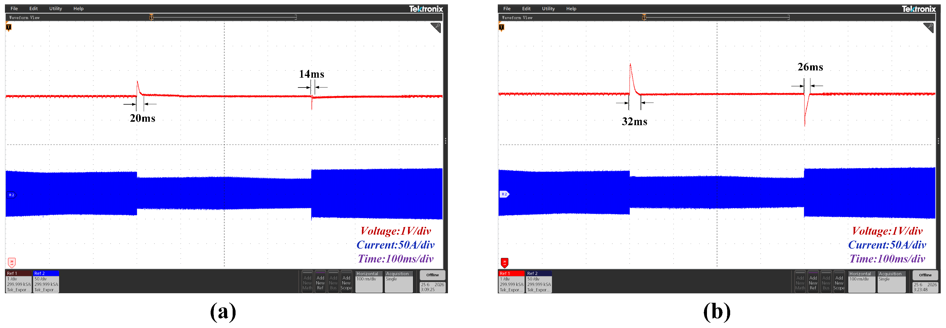The corresponding experimental waveforms are shown in Figure 21, where panels (a) and (b) correspond to GWO-FOMPC and IOMPC, respectively.

The load transitions cause temporary output-voltage and resonant-current deviations. GWO-FOMPC returns to the regulation band in approximately 20 ms and 14 ms, whereas IOMPC requires approximately 32 ms and 26 ms. The resulting settling-time reductions are 37.5% and 46.2%, respectively. The responses remain bounded during both transitions, supporting the load-adaptation capability of the converter-level control system over the tested range.

The measured settling times for all converter-level experimental transitions are summarized in

Table 10. Measured output-voltage settling times in the converter-level experiments.

Experimental Transition	IOMPC (ms)	GWO-FOMPC (ms)	Reduction (%)
$V_{\mathrm{in}}$: $100\to 110$ V	28	12	57.1
$V_{\mathrm{in}}$: $110\to 100$ V	36	26	27.8
$V_o^{*}$: $250\to 240$ V	18	11	38.9
$V_o^{*}$: $240\to 260$ V	22	16	27.3
$R_L$: $25\to 50\mathrm{\Omega }$	32	20	37.5
$R_L$: $50\to 22\mathrm{\Omega }$	26	14	46.2
Mean settling time	27.0	16.5	38.9

.

The hardware comparison is intentionally limited to IOMPC and GWO-FOMPC. The five-controller switching-level simulations are used to separate the effects of fractional-order augmentation and offline GWO tuning, whereas the hardware tests verify that the baseline and proposed endpoint controllers preserve their relative dynamic behavior on the same prototype. The agreement is qualitative rather than exact because the simulation omits part of the semiconductor, magnetic, sensing, and timing nonidealities present in the prototype.

5.5. Estimated Loss Distribution and Measured Efficiency

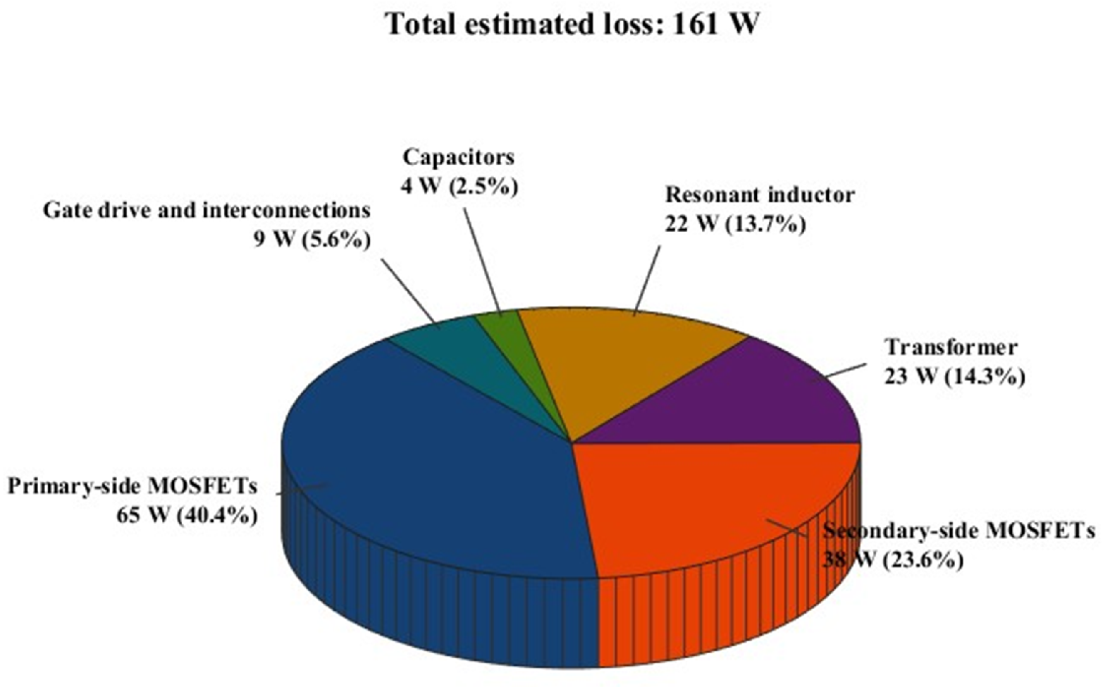
A component-level loss analysis was conducted using the steady-state electrical stresses under GWO-FOMPC at the nominal operating point of $V_{\mathrm{in}}=100$ V, $V_o=250$ V, $f_s=100$ kHz, and $P_o=2.5$ kW. The semiconductor losses were estimated from the datasheet-based conduction and switching characteristics of the primary- and secondary-side MOSFETs together with their corresponding electrical stresses. The estimated magnetic-component losses include the winding and core losses of the transformer and resonant inductor. The remaining losses are associated with the capacitors, gate-drive circuits, and interconnections.

Figure 22 shows the estimated loss distribution. The estimated losses of the primary-side MOSFETs, secondary-side MOSFETs, transformer, resonant inductor, capacitors, and gate-drive and interconnection circuits are approximately 65, 38, 23, 22, 4, and 9 W, respectively, giving a total estimated loss of approximately 161 W. Under the considered operating condition, the semiconductor devices represent the largest loss contribution, followed by the magnetic components.

The steady-state dc efficiency was measured at $V_{\mathrm{in}}=100$ V, $V_o=250$ V, and $f_s=100$ kHz. The electronic load was adjusted to obtain output-power levels of 0.5, 1.0, 1.5, 2.0, and 2.5 kW. After steady-state operation was reached, the input and output dc powers were calculated as

$$P_{\mathrm{in}}=V_{\mathrm{in}}{I}_{\mathrm{in}},P_o=V_o{I}_o,$$

(119)

and the conversion efficiency was determined from

$$\eta ={\displaystyle \frac{P_o}{P_{\mathrm{in}}}}\times 100\%.$$

(120)

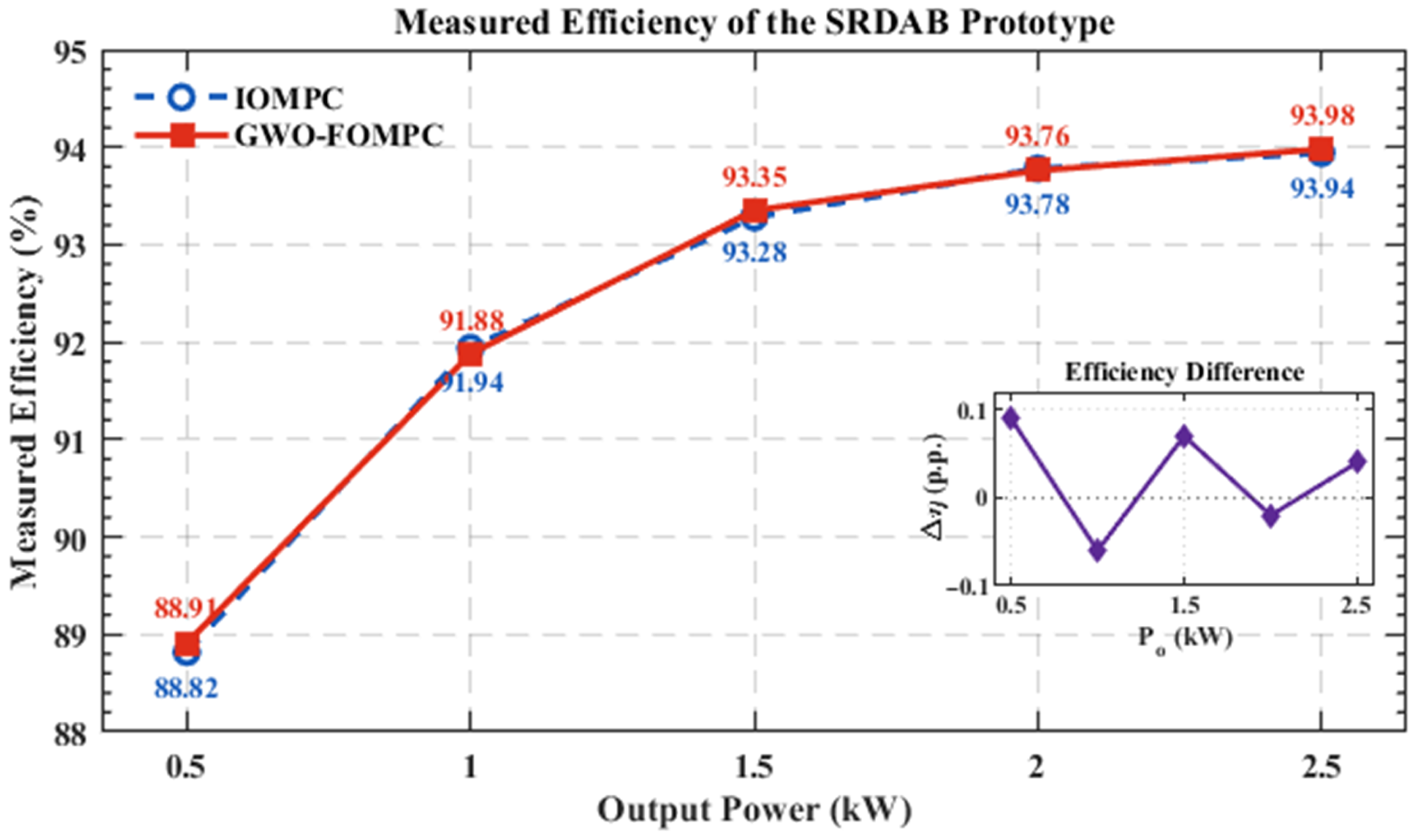
Figure 23 presents the measured steady-state efficiencies under IOMPC and GWO-FOMPC over the investigated output-power range. For both controllers, the measured efficiency increases with output power. At 2.5 kW, the measured efficiencies are 93.94% under IOMPC and 93.98% under GWO-FOMPC.

At 2.5 kW, the measured efficiency under GWO-FOMPC corresponds to a total converter loss of approximately 160.1 W. This result agrees closely with the component-level loss estimate of approximately 161 W.

6. Conclusions

This paper investigates an SRDAB-based isolated DC energy-sharing converter for temporary energy support of field medical electric vehicles. A control-oriented model is derived using the fundamental harmonic approximation, and a dual-loop GWO-FOMPC strategy is developed. The outer loop generates the reference power, while the predictive inner loop incorporates fractional-order finite-memory weighting into the integer-order physical model and analytically determines the constrained phase-shift angle. The controller parameters are tuned offline using the grey wolf optimizer.

The simulation and prototype results show improved dynamic performance under input-voltage, load, and output-voltage-reference variations. GWO-FOMPC achieves average and maximum settling times of 13.8 and 18 ms in simulation, respectively. In the experiments, the average settling time decreases from 27.0 ms with IOMPC to 16.5 ms, representing a reduction of 38.9%. The prototype reaches a measured efficiency of 93.98% at 2.5 kW.

The present study is limited to laboratory tests using programmable DC sources and an electronic load, primarily under unidirectional power transfer. Future work will integrate practical battery packs and battery management systems, investigate bidirectional operation and mode transitions, and evaluate a vehicle-level prototype under broader electrical and thermal conditions.