Article

Parameter Estimation of LFM Signals Based on PID-PSO-FRFT

1
Xi’an Key Laboratory of Active Photoelectric Imaging Detection Technology, Xi’an Technological University, Xi’an 710021, China
2
School of Optoelectronic Engineering, Xi’an Technological University, Xi’an 710021, China
*
Authors to whom correspondence should be addressed.
Fractal Fract. 2026, 10(3), 202; https://doi.org/10.3390/fractalfract10030202
Submission received: 12 February 2026 / Revised: 16 March 2026 / Accepted: 17 March 2026 / Published: 20 March 2026

Abstract

The fractional Fourier transform (FRFT) serves as an effective tool for linear frequency modulated (LFM) signal parameter estimation, whose performance depends on the search efficiency for the optimal transform order. To address the issues of fixed inertia weight in the standard particle swarm optimization (PSO) algorithm, which tends to fall into local optima and suffers from insufficient convergence accuracy, this paper introduces a proportional-integral-derivative (PID) control strategy and proposes a PID-PSO-FRFT-based LFM signal parameter estimation method. This approach introduces a PID controller, which takes the deviation between the particle’s current position and the global best position as input and dynamically adjusts the inertia weight through proportional, integral, and derivative regulation, thereby achieving an adaptive balance between global exploration and local exploitation capabilities of the particles. Simulation results demonstrate that, compared with the basic PSO-FRFT algorithm, the proposed method significantly improves the estimation accuracy of the center frequency and chirp rate of LFM signals under SNR conditions ranging from −9 dB to −7 dB, while considerably reducing computation time, exhibiting superior noise resistance, and exhibiting superior robustness.

1. Introduction

Linear frequency modulation (LFM) signals, characterized by a frequency that varies linearly over time, are a typical type of non-stationary signal [1]. They possess excellent time-domain and frequency-domain compression properties, as well as Doppler shift characteristics, leading to their widespread application in fields such as communications, sonar, seismic exploration, and biomedical engineering [2,3]. In practice, traditional spectral analysis methods based on the fast Fourier transform (FFT) are commonly used for parameter estimation of such signals. However, these methods fail to capture the time-varying frequency characteristics inherent to non-stationary signals. In contrast, time-frequency analysis methods can characterize the evolution of signal properties in both time and frequency domains, accurately capturing the distribution and variation in signal frequency at different time instants. Therefore, they are frequently employed for processing this class of non-stationary signals [4,5]. Common time-frequency analysis methods include the short-time Fourier transform (STFT), continuous wavelet transform (CWT), s-transform, and Wigner-Ville distribution (WVD), among others.
Among these, the STFT employs a fixed window function to perform segmented analysis of the signal. While computationally simple, the time-domain and frequency-domain concentration of the signal is simultaneously affected and constrained by the length of the window function, making it difficult for STFT to achieve both fine temporal and frequency resolution simultaneously [6,7]. The CWT adjusts the analysis resolution through variable scaling, possessing multi-resolution capability. However, the choice of the basis function significantly impacts the results, and there currently lacks a unified theory or criterion to guide the optimal selection of the basis function [8,9]. The S-transform combines characteristics of both STFT and CWT, improving time-frequency concentration to some extent through a frequency-adaptive window [10,11], but it comes with a relatively high computational cost [12,13]. The WVD, independent of window functions, achieves high time-frequency concentration [14]. However, its bilinear nature leads to the generation of cross-term interference when processing multi-component signals, which can easily mask the true signal characteristics [15,16].
In contrast, the fractional Fourier transform (FRFT) [17,18] demonstrates unique advantages in LFM signal processing. The FRFT can concentrate the energy of a linear frequency-modulated signal highly within a specific fractional domain, facilitating parameter detection and extraction [19,20]. Particularly when dealing with multi-component LFM signals, the FRFT does not suffer from the cross-term interference commonly associated with WVD-type methods [21,22], making FRFT-based LFM signal parameter estimation stand out among various methods [23].
However, the accuracy of the FRFT method largely depends on the search strategy for the optimal transformation order. Traditional grid search, while straightforward, suffers from issues of high computational load and limited resolution.
To reduce the search complexity of the optimal FRFT order, Shen et al. [24] proposed a two-stage coarse-to-fine TrTF-FrFT method, which narrows the FRFT search range via chirp rate coarse estimation from STFT time-frequency ridge extraction and completes fine search through FRFT domain Gaussian fitting. This method effectively reduces the computational cost, but it relies heavily on the validity of STFT coarse estimation: when the time-frequency ridge is submerged by noise at extremely low SNR or under large chirp rate conditions, the coarse estimation fails completely, making it inapplicable to non-cooperative reception scenarios without prior signal information. To overcome these limitations, swarm intelligence optimization algorithms can be introduced to leverage their powerful global optimization capabilities, thereby enhancing both the search efficiency and accuracy. Liu [25] combined particle swarm optimization (PSO) with the FRFT and successfully realized the Nyquist Zone identification and chirp rate estimation of the LFM signal intercepted by the Nyquist folding receiver, which fully verified the engineering effectiveness of the PSO algorithm in the global optimization of the optimal FRFT transform order. Meanwhile, to address the defects of traditional gradient-based optimization algorithms, namely their sensitivity to initial values and proneness to falling into local optima, Guo, Wang, et al. [26,27] proposed an FRFT-based method combining the simplified linear canonical transform with the water cycle algorithm. This method reduces the computational complexity of FRFT-based parameter estimation for LFM signals and also provides research insights for the performance improvement of swarm intelligence optimization algorithms. These studies have collectively validated the application value of swarm intelligence algorithms in FRFT-based LFM signal parameter estimation.
PSO, as a classic swarm intelligence optimization algorithm, has been widely applied to various optimization search problems since its introduction by Kennedy and Eberhart in 1995 [28]. This popularity stems from its advantages of simple structure, ease of implementation, fewer parameters, and rapid convergence. However, the performance of the standard PSO algorithm is highly dependent on the proper setting of its parameters, particularly the inertia weight ω—a key parameter that governs the balance between a particle’s global exploration and local exploitation capabilities. In traditional PSO, the inertia weight is often set as a fixed constant or adjusted using simple strategies such as linear decreasing. Such fixed or simplistic adjustment of inertia weight often struggles to balance global search capability with local fine-tuning when dealing with complex multi-modal, multi-constraint, or high-dimensional optimization problems. This limitation can easily lead to issues such as premature convergence or entrapment in local optima [29,30].
To address this issue, numerous studies have proposed various improvement strategies based on dynamically adjusting the inertia weight. Examples include exponential inertia weight and time-varying inertia weight [31,32]. Similar to linear decreasing strategies, these approaches guide particles to transition gradually from global search to local development through predefined functional forms, offering simple structures and easy implementation. Other strategies, such as random inertia weight [33], incorporate a stochastic mechanism to enhance particle diversity through random perturbations, thereby alleviating convergence issues to some extent. Additionally, chaos-based inertia weight methods [34] utilize chaotic maps or non-linear adjustments to leverage the ergodic properties of chaos, improving the ability to cover the search space and thus increasing the probability of the algorithm escaping local optima.
Although these improved strategies have enhanced the performance of the standard PSO to varying degrees, most methods still rely on empirical parameters or fixed adjustment rules, making it difficult to adaptively adjust the inertia weight in real time based on the state of the search process.
To address this issue, this paper introduces the proportional-integral-derivative (PID) control mechanism and further proposes a PID-PSO-FRFT-based method for LFM signal parameter estimation. This method introduces a PID controller, which takes the “deviation between the particle’s current position and the global best position” as the control input. Through the combined proportional, integral, and derivative regulation of the PID controller, the inertia weight is adaptively and dynamically adjusted in real-time. This adjustment modifies the particle’s velocity update strategy. Through iterative search, the optimal transformation order for the FRFT is determined. Subsequently, based on the analytical relationship between this optimal order and the chirp rate and initial frequency of the LFM signal, the accurate estimation of the signal parameters is ultimately achieved.
The structure of this paper is organized as follows: Section 1 is the Introduction; Section 2 details the LFM Signal Parameter Estimation Method Based on PID-PSO-FRFT; Section 3 presents the Simulation Experiments and Result Analysis; Section 4 is the Conclusion.

2. LFM Signal Parameter Estimation Based on PID-PSO-FRFT

2.1. Signal Model

In this subsection, we introduce the LFM signal model. The formula is as follows [22]:
x ( t ) = s ( t ) + n ( t )
Here,   n ( t ) represents Gaussian white noise, indicates environmental interference with the signal, and   s ( t ) denotes the LFM signal, which can be modeled as:
s ( t ) = A exp ( j 2 π f 0 t + π k t 2 ) , T / 2 t T / 2
where A ,   f 0 ,   k ,   T represent the amplitude, center frequency, chirp rate, and modulation period of the LFM signal, respectively.
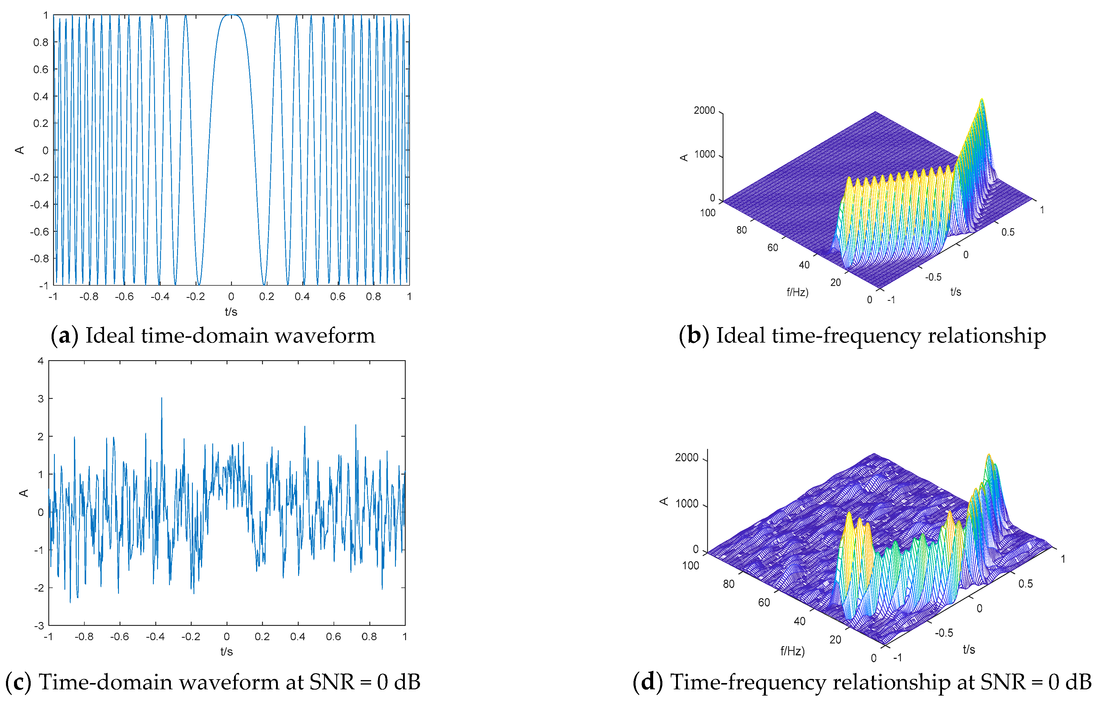
Assuming the LFM signal parameters are set as A = 1 ,   T [ 1,1 ] ,   k = 30 ,   f 0 = 0 , the time-domain waveform and the time-frequency relationship of the signal are illustrated in the following figure.
From the time-domain waveform in Figure 1a, it can be observed that the density of the signal waveform varies regularly over time: in this example, since k > 0, the waveform gradually becomes denser from left to right, corresponding to a linear increase in instantaneous frequency, while the opposite occurs on the negative half-axis. The time-frequency relationship in Figure 1b more directly illustrates the time-frequency coupling characteristic of the LFM signal: the straight line with a slope of k = 30 clearly demonstrates the linear variation in instantaneous frequency over time, which fundamentally differs from the horizontal straight line characteristic of a single-frequency signal’s time-frequency figure.
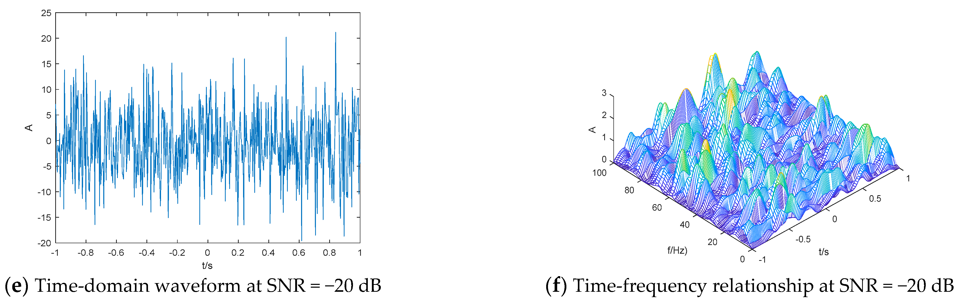
In Figure 1c,d, noise obscures the time-domain waveform, making it difficult to discern. However, time-frequency analysis can still extract the frequency evolution trajectory. Nevertheless, affected by noise interference, the energy distribution in Figure 1d exhibits significant dispersion, and the clarity of the time-frequency ridge line and the degree of energy concentration are reduced compared to Figure 1b, reflecting the weakening effect of noise on energy aggregation.
In Figure 1e,f, as the SNR further decreases to −20 dB, strong noise completely masks the regular variation in the LFM signal, rendering the time-domain waveform unidentifiable. In the corresponding time-frequency relationship figure, the dispersion of energy distribution intensifies, the time-frequency ridge line is entirely obscured, and energy concentration is completely lost. This visually demonstrates the severe interference of noise on time-frequency analysis under low SNR conditions.

2.2. Principle of LFM Signal Parameter Estimation Based on FRFT

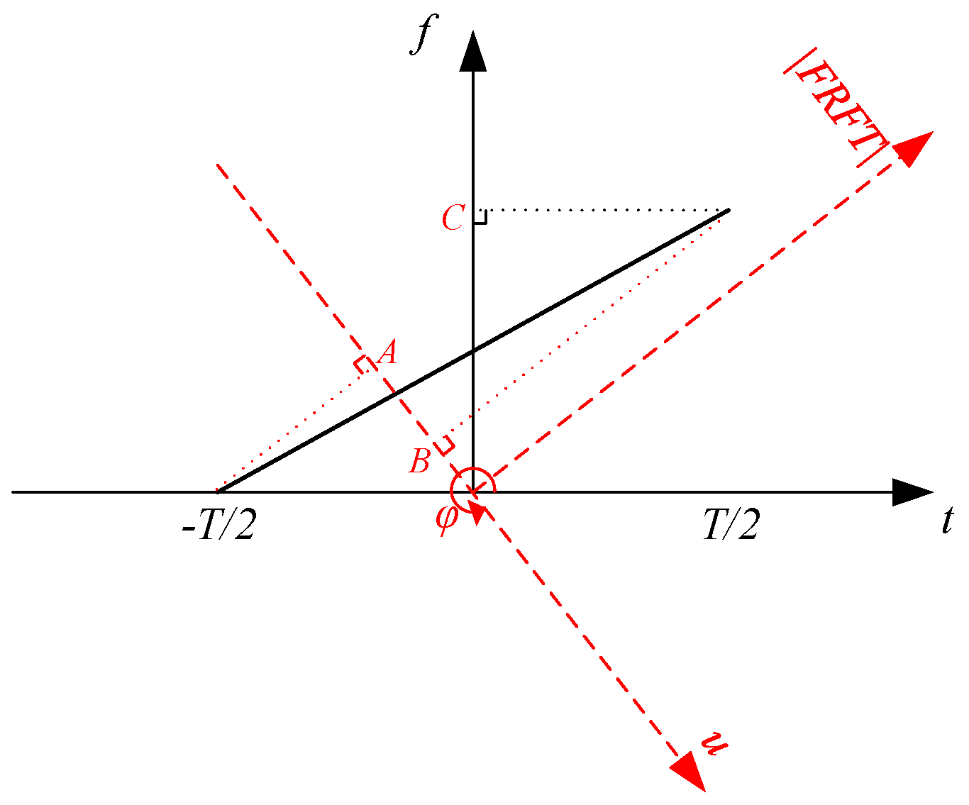
The Fractional Fourier Transform (FRFT), also known as the angular Fourier transform or rotational Fourier transform, generates a fractional domain coordinate system. This coordinate system has a rotational relationship relative to the original time-frequency plane coordinate system [35]. The time-frequency line of an LFM signal is transformed from the original time-frequency plane into this fractional domain coordinate system, as illustrated in Figure 2.
In the original time-frequency plane with the time axis t and the frequency axis f as its basis, the time-frequency curve of the LFM signal is shown in the figure above. When performing a p-order FRFT on the signal, it can be considered as rotating the entire time-frequency coordinate system around the origin by an angle φ = (π/2)p, where p is the order of the FRFT. After rotation, we obtain a new fractional domain coordinate axis u, which is the unique independent variable of the FRFT output signal transformed from the original time axis; The projection distribution of the time-frequency curve on this new axis u corresponds to the FRFT result of the signal.
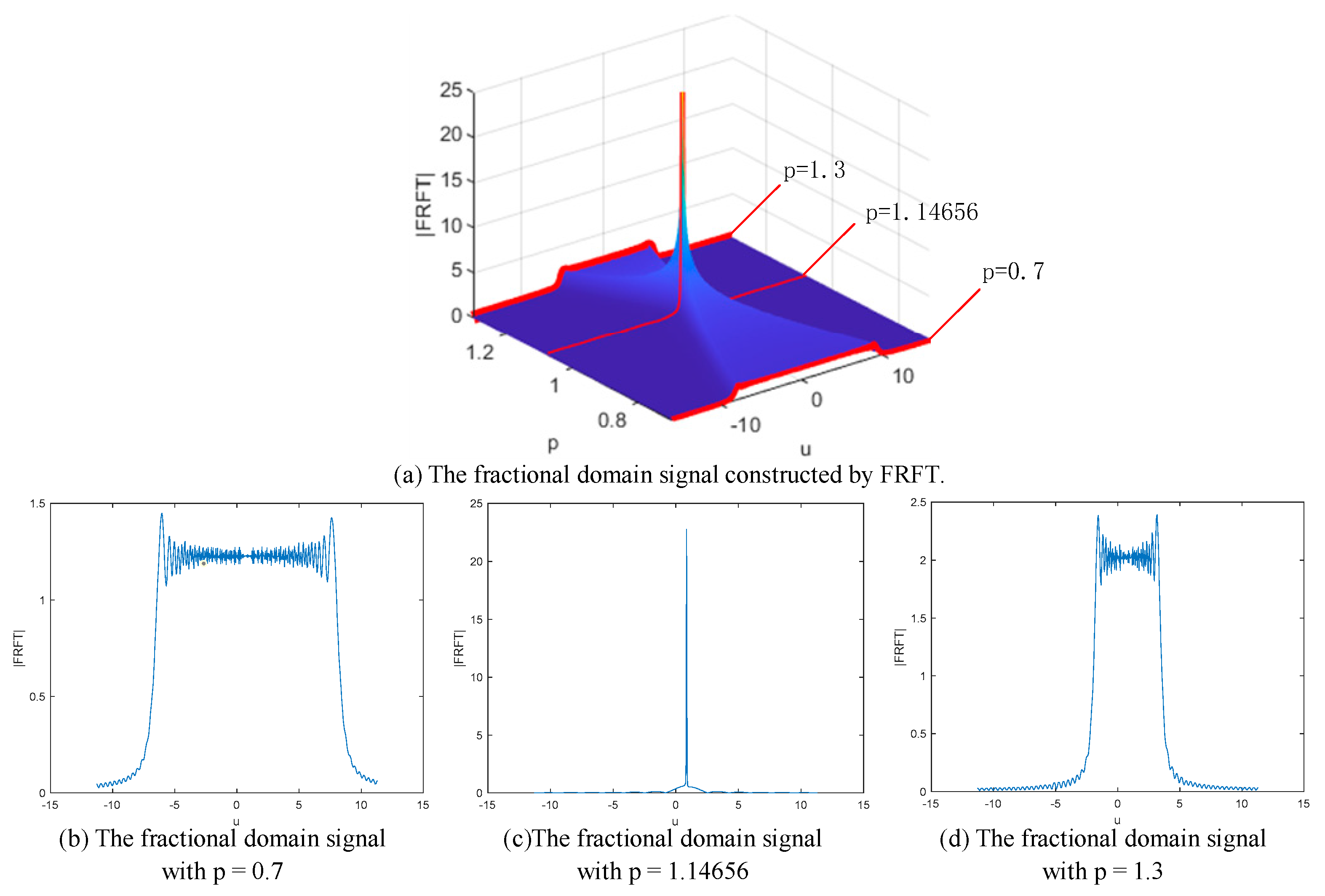
For an ideal LFM signal, its energy is uniformly distributed across the projection interval [A, B] of its time-frequency line on the u-axis. A narrower projection interval [A, B] indicates higher energy concentration. When the u-axis is perpendicular to the ideal LFM signal’s time-frequency line, the projection collapses to a single point, achieving the highest possible energy concentration. Leveraging this characteristic, the FRFT method enables parameter estimation of LFM signals. When the signal energy in the fractional domain converges into an impulse-like signal, the corresponding transformation order p is the optimal FRFT order for the LFM signal. The energy concentration of the LFM signal after applying FRFTs of different orders is illustrated in Figure 3.
The p -th order FRFT of an LFM signal x ( t )   is defined as follows [36,37]:
X p ( u ) = F p [ x ( t ) ] = x ( t ) K p ( t , u ) d t
The kernel function K p ( t , u ) is given by:
K p ( t , u ) = A φ exp ( j π ( t 2 + u 2 ) cot φ j 2 π u t csc φ ) φ n π δ ( t u ) φ = 2 n π δ ( t + u ) φ = ( 2 n + 1 ) π
where A φ = 1 j c o t φ , n = 1,2 , 3 ., φ = ( π / 2 ) p represents the rotation angle of the time-frequency plane, F p denotes the FRFT operator, and δ ( t ) is the unit impulse function.
According to the reference [37], the definition of FRFT can be simplified to the following expression:
X p ( u ) = A φ y ( t ) exp [ j π ( u 2 + t 2 ) cot φ j 2 π u t csc φ ] d t
To establish a connection between the theoretical formulation of the fractional Fourier transform (FRFT) and its practical engineering applications, researchers have investigated various discretization schemes for its implementation. There are numerous approaches to discretizing the FRFT. Among them, the method proposed in reference [38], which utilizes the FFT to compute the convolution in the time-frequency domain without requiring Fresnel integrals, reduces computational complexity. It is considered one of the fastest methods and is suitable for real-time computation of discrete signals. All simulations in this paper strictly adopt this algorithm, and the entire implementation fully follows the standard calculation process, normalization convention, and discrete index-to-fractional-domain u mapping rules defined in the original reference [38]. Furthermore, due to the different physical dimensions of time and frequency, numerical computation of the FRFT cannot correctly map the signal to the fractional domain, leading to deviations in signal parameter estimation results [39,40]. Therefore, the signal’s time and frequency must be transformed into a unified dimensionless domain. The normalization factor S is given by the following equation.
S = T f s 1 2
where T   is the time width of the LFM signal, and f s is its sampling frequency. The new coordinates after dimensional normalization are given by:
t = t / S f = f S
The discretization method of FRFT adopted is as follows (Figure 4):
Using the estimated optimal order p ^ and the sampling point u ^ corresponding to the peak of the signal impulse in the fractional domain at this optimal order, the center frequency f 0 and the chirp rate k of the LFM signal can be computed as follows:
φ ^ = π 2 p ^
f 0 = u ^ csc φ ^
k ^ = cot φ ^
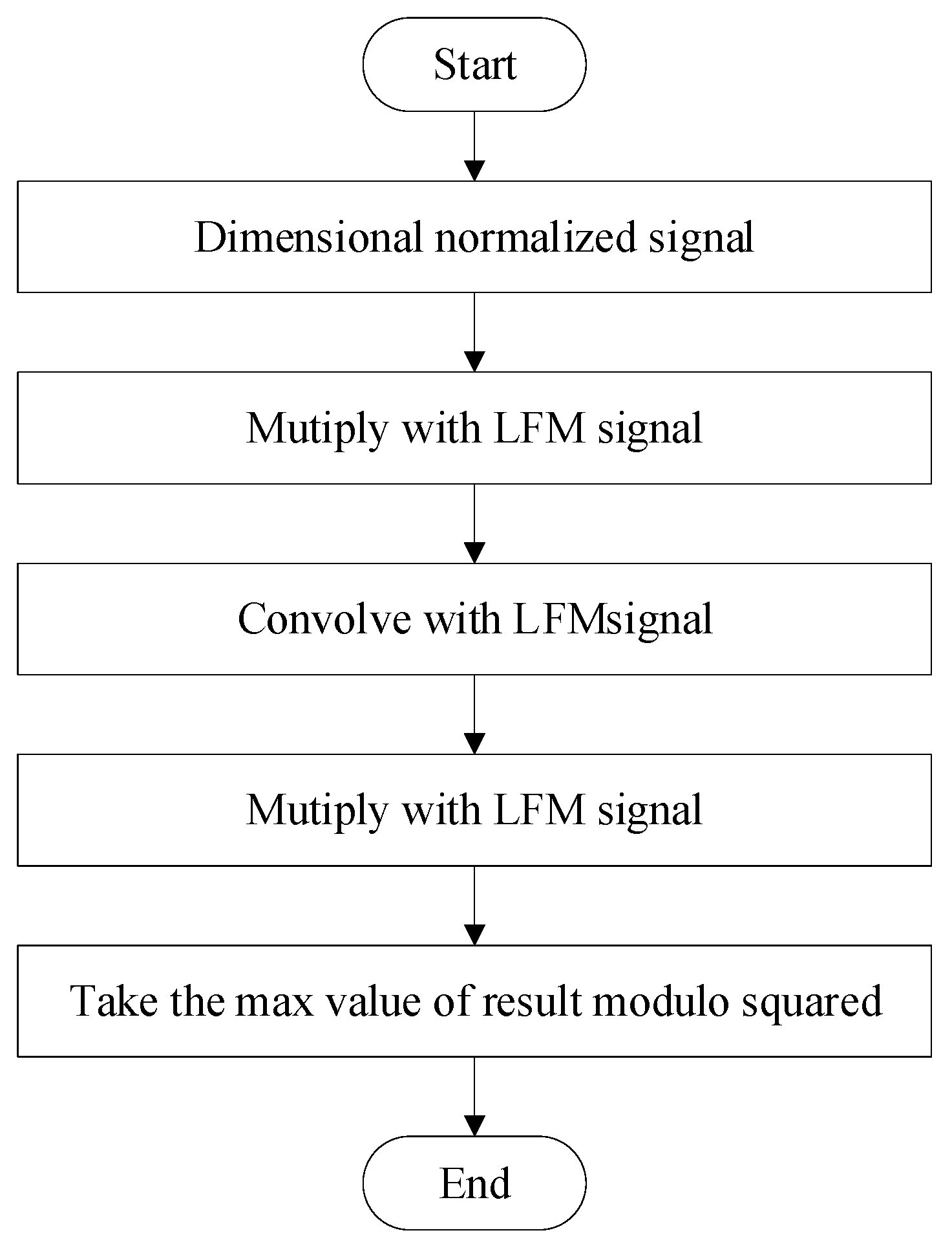
In summary, to clearly demonstrate the entire implementation process of the proposed method, the full step-by-step workflow and execution flowchart for FRFT-based parameter estimation of LFM signals are systematically organized and detailed in Figure 5.

2.3. Principle of the PID-PSO-FRFT Algorithm

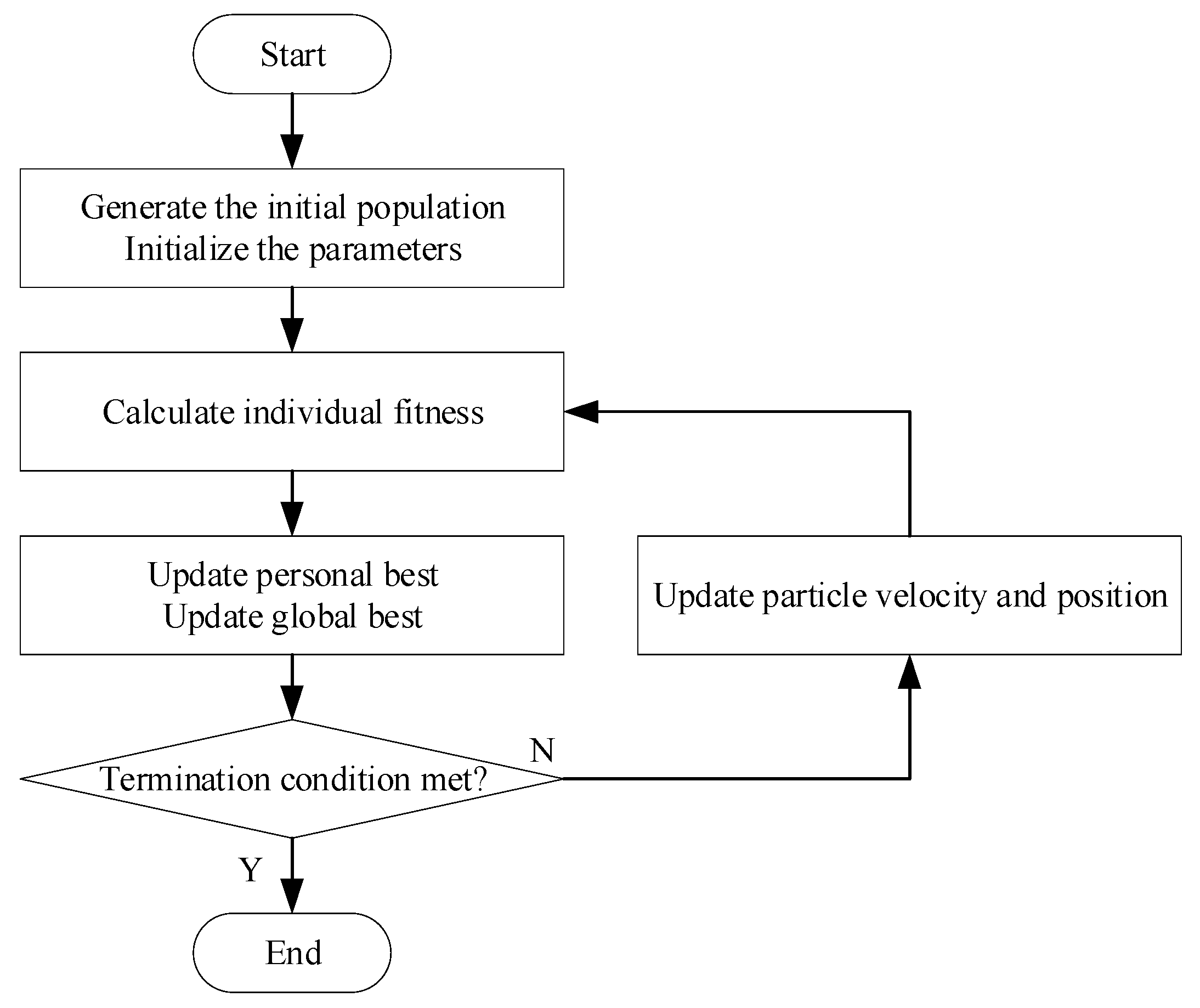
The PSO algorithm simulates the foraging behavior of bird flocks. Each particle in the algorithm is considered an independent bird individual, while the search space of the parameters to be optimized corresponds to the foraging area. Particles dynamically adjust their search direction and step size based on individual experience and group information. The fitness function is used to evaluate the quality of the current position, and particles continuously update their states accordingly. Ultimately, the algorithm searches for the optimal position across the entire search space. The flowchart of the PSO algorithm is shown in Figure 6.
First, initialize the population and parameters, including the total number of particles in the population, individual dimension, initial positions (corresponding to the transformation orders of FRFT), and initial velocities (step sizes) of the particles, as well as the maximum iteration count of the algorithm. Set the PID control parameters, including the proportional coefficient K p , integral coefficient K i , differential coefficient K d , and the search range for the optimal FRFT order. Among these, since the Fractional Fourier Transform contains a cot φ term, which tends to infinity when φ approaches integer multiples of π / 2 , the search range must be constrained to a bounded and solvable safe interval. According to the rigorous derivation in the existing references [22,37], the search range is calculated as follows:
p 0 = 2 π arccot ( 1 2 ) p 1 = 2 p 0
where p 0 is the minimum effective order, p 1 is the maximum effective order. Numerically, this yields p0 ≈ 0.7048 and p1 ≈ 1.2952, Based on the rigorous derivation from the existing references [22,37], the search range for the optimal FRFT order can be reasonably set to p ∈ (0.7, 1.3) to cover the theoretical optimal order while avoiding numerical singularities.
Assuming a population consists of N particles, during the t -th iteration of the optimization process, particle x i updates its velocity and position according to the following equations [29,32]:
v i ( t + 1 ) = ω v i ( t ) + c 1 r 1 ( p b i x i ( t ) ) + c 2 r 2 ( g b x i ( t ) ) x i ( t + 1 ) = x i ( t ) + v i ( t + 1 )
Here, i = 1,2 , , N , denotes the i -th particle in the entire population; c 1 is the individual learning factor, indicating the influence of the particle’s own information on its optimization; c 2 is the social learning factor, representing the influence of other particles in the population on its optimization. Together, c 1 and c 2 are referred to as learning factors, both being non-negative constants. r 1 and r 2 are random numbers uniformly distributed in [0, 1]. ω is the inertia weight coefficient, indicating the proportion of the previous iteration’s velocity retained in the current iteration. Increasing ω enhances the particle’s inheritance of historical velocity, thereby strengthening the algorithm’s global search capability, which helps escape local optima and improves global exploration. Conversely, decreasing ω reinforces the particle’s local exploitation ability, thereby improving solution accuracy and convergence efficiency.
In the traditional PSO algorithm, the inertia weight coefficient is typically set as a fixed value or linearly decreasing, making it difficult to dynamically balance global exploration and local exploitation during algorithm iterations. This often leads to the algorithm becoming trapped in local optima or suffering from insufficient convergence accuracy. In contrast, the PID-PSO algorithm introduces a PID controller to dynamically adjust the inertia weight ω, achieving an adaptive balance between “global exploration” and “local exploitation.” The adaptive update rule for the inertia weight ω is given as follows:
Calculation of the inertia weight ω. The dynamic inertia weight is obtained by subtracting the total PID correction term from the upper limit of the inertia weight, as expressed in the following formula:
ω ( i ) = ω max P I D ( i ) , ω ( i ) [ ω min , ω max ]
where ω ( i ) is the dynamic inertia weight corresponding to the i -th particle; ω max is the upper limit and ω min is the lower limit of the inertia weight. Presetting the boundary [ ω min , ω max ] prevents ω from becoming too large or too small, which could lead to an imbalance in the particle’s search capability; PID ( i ) is the total PID correction term for the i -th particle, controlled through proportional, integral, and derivative components, calculated as follows:
P I D ( i ) = P ( i ) + I ( i ) + D ( i )
Here, P ( i ) , I ( i ) , and D ( i ) represent the proportional, integral, and derivative output terms for the i -th particle, respectively. They are calculated as:
P ( i ) = K p e _ c u r r e n t ( i ) I ( i ) = K i e s u m ( i ) D ( i ) = K d [ e _ c u r r e n t ( i ) e p r e ( i ) ] , i = 1 , 2 , 3 , , N .
Here, K p , K i , and K d denote the proportional, integral, and derivative coefficients, respectively; e sum ( i ) is the cumulative sum of e current for the i -th particle from the first generation to the current iteration; e pre ( i ) is the e current value of the i -th particle from the previous iteration; e current represents the deviation between the particle’s current position and the global best position, defined as:
e _ c u r r e n t ( i ) = g b e s t x ( i ) , i = 1 , 2 , , N
In the equation, e current ( i ) denotes the current position deviation of the i -th particle; g b e s t is the global best position (i.e., the current globally optimal FRFT order) found by the PSO algorithm up to the current generation; x ( i ) represents the current position of the i -th particle; and N is the total number of particles in the swarm.
In each iteration, the state of each particle is updated, and its individual historical best position as well as the global historical best position are also adjusted accordingly. Assuming the optimization problem is to find the minimum of the objective function f ( x ) , various methods can be employed to construct the objective function f ( x ) for evaluating the transformation results in the FRFT optimal order search—that is, for fitness calculation. Among these, the maximum value method is one of the most commonly used due to its simplicity and practicality. The objective function f ( x ) corresponding to the maximum value method is given as follows [21,22]:
f ( x ) = max ( X p ( u ) 2 )
Then, in each iteration, from the start of the algorithm up to the t -th iteration, according to the standard particle swarm optimization framework [30,33], the update equation for the individual historical best position of a particle and the global historical best position of the entire population are as follows.
p b i ( t + 1 ) = x i ( t + 1 ) f ( x i ( t + 1 ) ) < f ( p b i ( t ) ) p b i ( t ) f ( x i ( t + 1 ) ) f ( p b i ( t ) )
g b = g b f ( p b i ) f ( g b ) p b i f ( p b i ) < f ( g b )
All particles in the population explore the solution space and update their states as the number of iterations increases. Under such circumstances, it is necessary to impose additional constraints beyond the rules governing particle velocity and displacement; otherwise, excessive particle movement may lead them beyond the solution space. Typically, the velocity v i of each particle is limited within [ v min , v max ] , and its position x i is confined within [ x min , x max ] . When a particle exceeds these boundaries, corresponding corrective measures are applied to ensure that each particle conducts its search within a meaningful solution space.
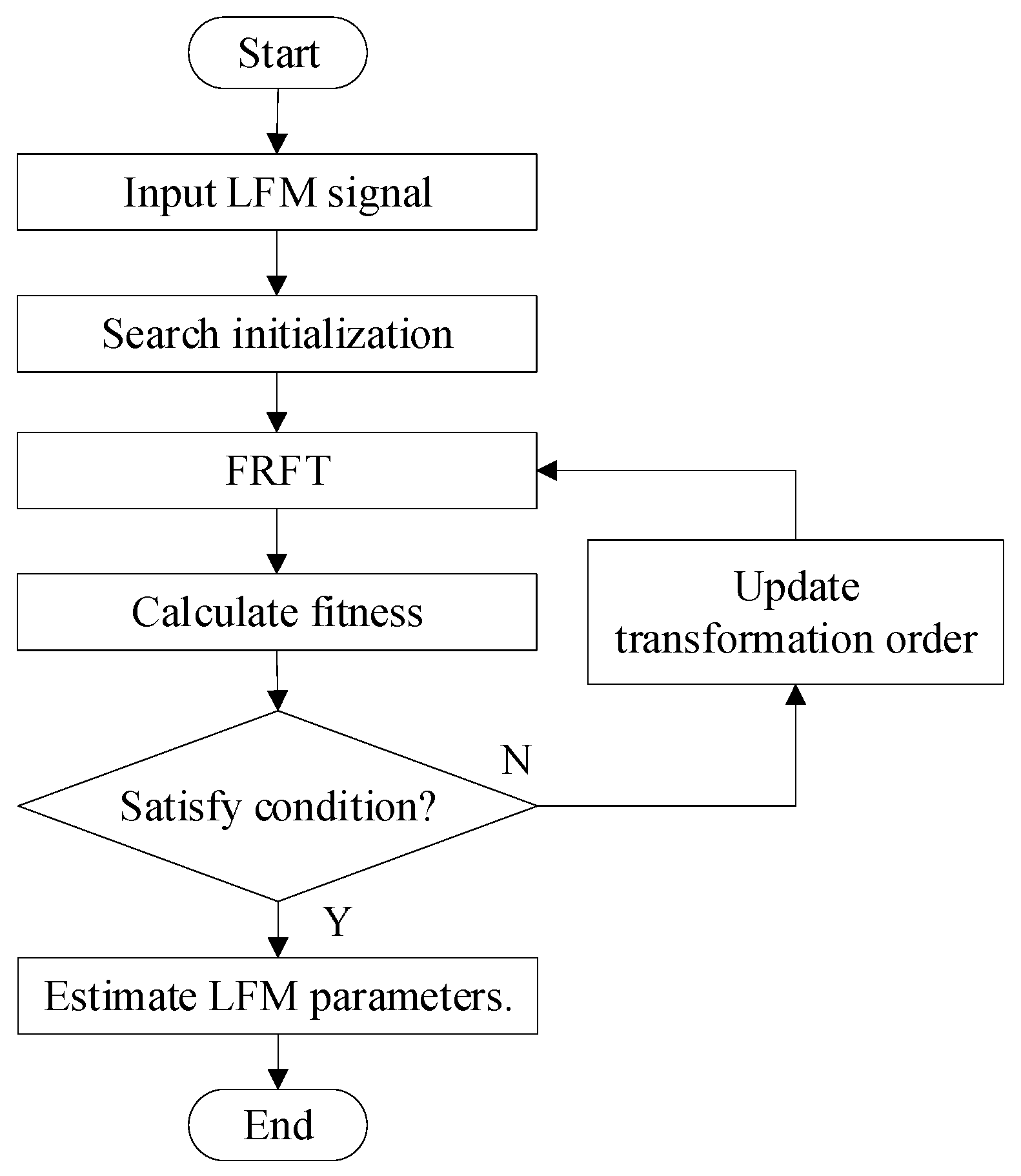
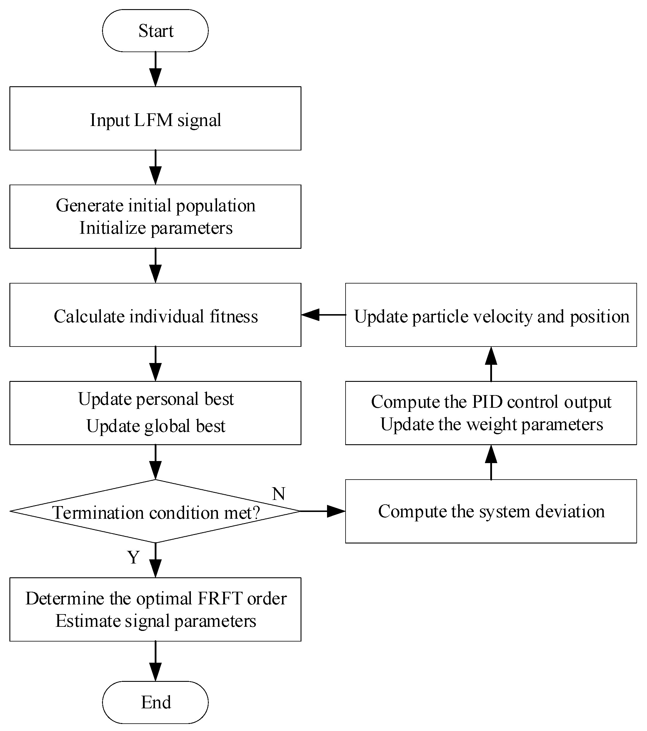
The flowchart of the PID-PSO-FRFT algorithm is illustrated in Figure 7.
In summary, the workflow of the PID-PSO-FRFT algorithm is as follows:
Step 1: Initialize all particles of the entire population within the solution space, including the total number of particles in the population, individual dimensions, initial positions (corresponding to FRFT transformation orders), initial velocities (step sizes), and the maximum number of iterations for the algorithm. Set the PID control parameters, including the proportional coefficient K p , integral coefficient K i , and differential coefficient K d . Determine the search range for the optimal FRFT order.
Step 2: Calculate the fitness value of each particle in the population based on its individual position (transformation order) and the evaluation function.
Step 3: Compare the current fitness value f current of each particle with its historical best fitness value f pbest . If f current is superior to f pbest , update f pbest = f current and record the corresponding solution as the local best solution. Otherwise, keep f pbest unchanged.
Step 4: Compare the particle’s fitness value f current with the historical global best fitness value f gbest of the entire population. If f current is superior to f gbest , update f gbest = f current . Otherwise, keep f gbest unchanged.
Step 5: Check whether the current global best solution satisfies the algorithm termination condition. If not, calculate the PID output to dynamically adjust the inertia weight ω for updating particle velocities. Update each particle’s position and velocity. If any particle moves beyond the feasible solution space, apply predefined rules for correction, then return to Step 2.
Step 6: If the termination condition is satisfied, return the global best solution, i.e., the optimal FRFT transformation order, completing the optimization process and concluding the search. A pseudocode representation of the algorithm is provided below (Algorithm 1):
Algorithm 1. PID-PSO-FRFT
Input: LFM signal s, The time series corresponding to the signal t
Output :   Chirp   rate   k ^   and   center   frequency   f ^ 0 of the LFM Signal
1: Initialization:
    Number of particles: n;
    Maximum iteration count: T m a x ;
    Position bounds: [ x m i n , x m a x ] ;
     Velocity   bounds :   [ v min , v max ] ;
    PID parameters: K p , K i , K d ;
    Inertia weight bounds: [ ω m i n , ω m a x ] ;
     Randomly   initialize   particle   positions :   x i [ x m i n , x m a x ] i = 1, …, n;
     Initialize   velocities :   v i ← 0;
     Individual   best :   p i x i ;
     Initialize   individual   best   fitness :   f i p b e s t ←−∞;
    Initialize global best: gb←∅ ; f g b e s t ←−∞;
     Initialize   PID   errors :   e s u m 0 ;   e p r e v ←0;
     Inertia   weight :   ω
2: for iter = 1 to Tmax do
3:           for i = 1 to n do
4:                                         f i   max ( | FRFT ( s , x i )|)     //Calculate fitness
5:                                     if   f i   >   f i p b e s t then     //Update individual best
6:                                                       p i   x i ,   f i p b e s t   f i
7:            end if
8:         end for
9:                           f c u r r   max ( f i p b e s t )     //Update current best
10:                       i *     argmax   f i p b e s t
11:                       if   f c u r r   >   f g b e s t then
12:                                     gb   x i * ,   f g b e s t   f c u r r     //Update historical best
13:      end if
14:                       if   f g b e s t ≥ threshold then     //Fitness threshold judgment
15:     break
16:        end if
17:         // Adaptive PID adjustment
18:                       e c u r r ← g-x     //Current error
19:                       P   K p · e c u r r     //Proportional term
20:                       e s u m e s u m + e c u r r
21:                       I   K i · e s u m      //Integral term
22:                       D   K d · ( e c u r r - e p r e v )     //Derivative term
23:         Δ ω ← P+I+D     //PID correction term
24:         ω   ω - Δ ω
25:         ω clip ( ω , ω m i n , ω m a x )     //Boundary Constraint
26:        // Particle Update
27:        v ← ω ·v+c_1·(p−x)+c_2·(g−x)
28:        v ← clip(v, v m i n , v m a x )
29:        x ← x+v
30:        x ← clip(x, x m i n , x m a x )
31:                       e p r e v e c u r r      //Update Error Record
32: end for
33: // Calculate the chirp rate and center frequency of the LFM signal based on gb
34: k ^ , f ^ 0 ←calculate_lfmParam(gb)
35: return k ^ & f ^ 0

3. Simulation Experiments and Analysis

3.1. Experiment 1: Comparative Experiment on Anti-Noise Robustness of LFM Signal Parameter Estimation Algorithms Under Different SNRs

To analyze the estimation accuracy of the basic PSO-FRFT algorithm, the PID-PSO-FRFT algorithm, and other PSO variants with different inertia weight strategies for LFM signal parameters under different Signal-to-Noise Ratios (SNRs), all algorithms were employed to perform 1000 Monte Carlo experiments on LFM signals embedded in Gaussian white noise with different SNRs. The experiments focused on parameter estimation of the LFM signal’s center frequency f 0 and chirp rate k .
The inertia weight update equations of the Linear-PSO and Exp-PSO methods are given as follows:
Linear-PSO:
ω = ω m a x ( ω m a x ω m i n ) i t e r m a x i t e r
where ω m a x and ω m i n are the initial maximum and final minimum values of the inertia weight, respectively, iter is the current iteration number, and m a x i t e r is the maximum number of iterations.
Exp-PSO:
ω = ω m a x ( ω m i n ω m a x ) i t e r m a x i t e r
The symbols in this formula have the same meanings as those in the Linear-PSO, and the nonlinear decreasing of the inertia weight is realized through the exponential form.
The common parameter settings for the basic PSO-FRFT, PID-PSO-FRFT, linear decreasing inertia weight PSO (Linear-PSO), and exponential decreasing inertia weight PSO (Exp-PSO) algorithms (excluding the inertia weight ω) are shown in Table 1.
The differences in inertia weight ω settings and additional tuning parameters of each algorithm are listed in Table 2.
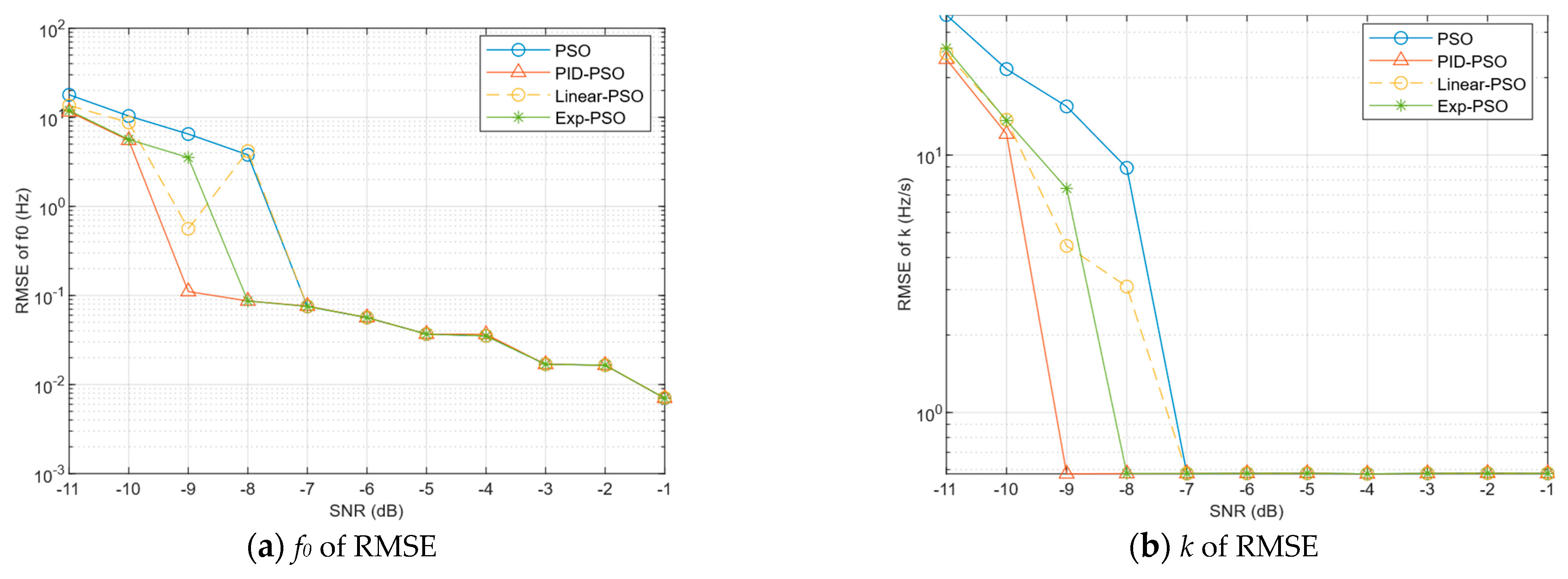
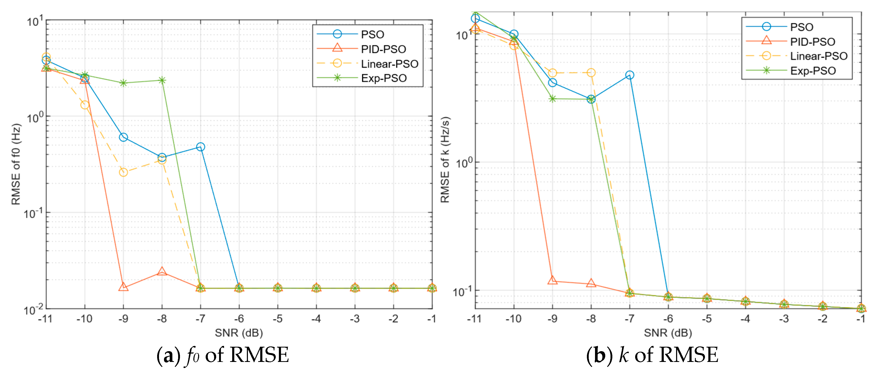
Assume the parameters of the LFM signal are A = 1 , f 0 = 70 , k = 60 , T = 2 , and the number of sampling points N = 512 . The SNR = { 11 , 10 , 9 , 8 , 7 , 6 , 5 , 4 , 3 , 2 , 1 } . The following figure presents the RMSE of the parameter estimation for the center frequency f 0 and chirp rate k of LFM signals, obtained by different PSO variants under different SNR conditions, with all results calculated from 1000 independent Monte Carlo simulation trials.
Assume the parameters of the LFM signal are A = 1 , f 0 = 10 , k = 30 , T = 2 , and the number of sampling points N = 512 . The SNR = { 11 , 10 , 9 , 8 , 7 , 6 , 5 , 4 , 3 , 2 , 1 } . The following figure presents the RMSE of the parameter estimation for the center frequency f 0 and chirp rate k of LFM signals, obtained by different PSO variants under varying SNR conditions, with all results calculated from 1000 independent Monte Carlo simulation trials.
It can be seen from Figure 8 that when SNR ≥ −7 dB, the RMSE of parameter estimation for all four algorithms converges to an extremely low level, and all algorithms can achieve high-precision and effective estimation of the center frequency f 0 and chirp rate k of the LFM signal. As the SNR decreases, when the SNR falls within the interval of [−9 dB, −8 dB], the RMSE of parameter estimation of the basic PSO algorithm rises sharply, and its optimization performance is completely invalidated. Although the Linear-PSO and Exp-PSO algorithms achieve a certain performance improvement compared with the basic PSO algorithm, they still present a significant abrupt increase in estimation error. In sharp contrast, the PID-PSO algorithm proposed in this paper still maintains extremely high parameter estimation accuracy in this interval: the RMSE of the center frequency f 0 sustains at the order of 10−1, and the estimated RMSE of the chirp rate k also remains below 100. It is not until the SNR drops to a lower level that the performance of the proposed algorithm begins to deteriorate abruptly.
It can be seen from the variation law of the curves in Figure 9 that the performance variation trend of each algorithm is highly consistent with that in Figure 8. When SNR ≥ −6 dB, the RMSE of parameter estimation for all four algorithms converges to an extremely low level, and all algorithms can achieve effective estimation of LFM signal parameters. As the SNR decreases to the interval of [−9 dB, −7 dB], the estimation error of the basic PSO algorithm first jumps by orders of magnitude, and its optimization performance is completely invalidated. Although the Linear-PSO and Exp-PSO algorithms achieve a certain performance improvement compared with the basic PSO algorithm, they still cannot avoid the sharp increase in estimation error and maintain effective estimation, with their performance abruptly failing when SNR < −7 dB. In sharp contrast, the PID-PSO algorithm proposed in this paper still maintains strong optimization stability in this interval: the RMSE of the estimation for the center frequency and chirp rate remains at a low magnitude level, and the performance of the proposed algorithm shows significant attenuation only when the SNR drops below −9 dB.
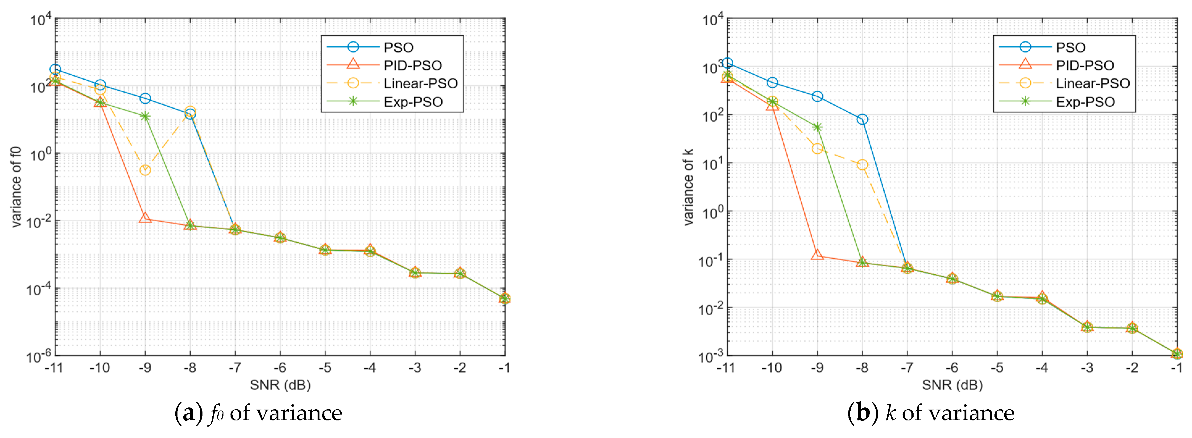
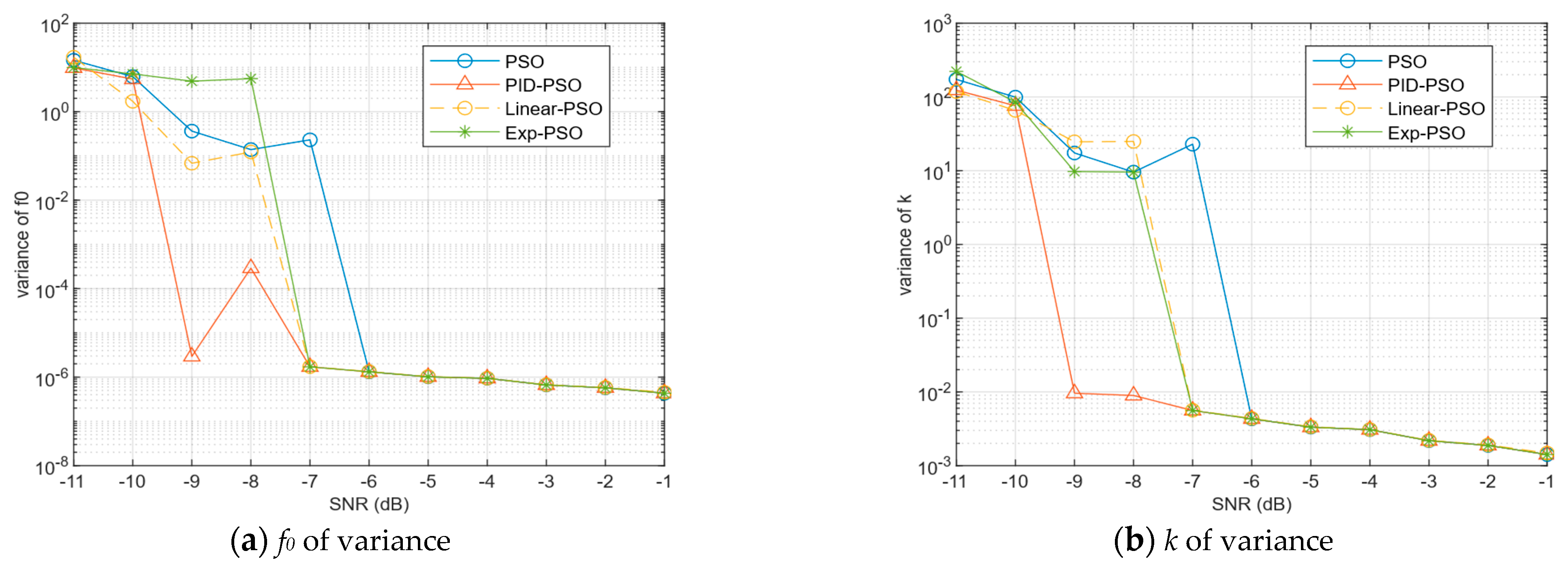
Based on the 1000 independent Monte Carlo experiments corresponding to the test in Figure 8, we further supplement the variance statistics of the center frequency f0 and chirp rate k estimated by each algorithm under different SNR conditions to quantitatively evaluate the dispersion and robustness of the estimation results, as shown in Figure 10.
The results show that the parameter estimation variance of all four algorithms decreases significantly with the increase in SNR; when SNR ≥ −7 dB, the estimation variance of all algorithms converges to a low magnitude, and stable parameter estimation can be achieved by all methods. However, when the SNR drops to the low SNR interval of [−9 dB, −8 dB], the estimation variance of the traditional PSO, Linear-PSO, and Exp-PSO algorithms jumps by orders of magnitude, leading to severe dispersion and instability of the estimation results, while the PID-PSO algorithm proposed in this paper can still maintain the estimation variance at a low magnitude without obvious stability deterioration.
The variance statistics from 1000 Monte Carlo simulations, which correspond to the LFM parameter estimation results in Figure 9, are shown below (Figure 11).
Figure 11. Variance of estimated f0 and k under different SNRs (LFM: f0 = 10, k = 30).
Fractalfract 10 00202 g011
The results present a completely consistent variance variation trend with the previous test: when the SNR drops to the interval of [−9 dB, −7 dB], the estimation variance of the conventional PSO, Linear-PSO, and Exp-PSO jumps by orders of magnitude, while the proposed PID-PSO still maintains an extremely low estimation variance and stable estimation performance. This result is in good agreement with the RMSE analysis in Figure 9, fully verifying that the anti-noise robustness and estimation stability of the proposed algorithm are independent of the inherent parameters of the LFM signal, with favorable engineering universality.
The experimental results demonstrate that the advantages of the proposed PID-PSO algorithm in anti-noise robustness and parameter estimation performance are not affected by the changes in the inherent parameters of the LFM signal. The algorithm maintains stable performance in different LFM signal scenarios, which further verifies the engineering practicability and universality of the proposed algorithm.

3.2. Experiment 2: Comparative Experiment on Convergence Speed of LFM Parameter Estimation Under Different SNRs

To analyze the speed of the PID-PSO algorithm in searching for the optimal FRFT order for LFM signal parameter estimation, the theoretical fitness extreme value is calculated. Within the iterations, 99.8% of this extreme value is set as the fitness threshold; reaching this threshold is considered convergence, and the search stops. A total of 1000 independent Monte Carlo trials are performed for each SNR level.
To intuitively compare the performance improvement in convergence speed between the PID-PSO algorithm and the basic PSO algorithm, the speed-up ratio(sur) is used as an indicator. Its calculation formula is as follows:
S p e e d u p   R a t i o = [ ( a b ) / a ] 100 %
where a is the mean iteration count of the basic PSO algorithm, and b is the mean iteration count of the PID-PSO algorithm.
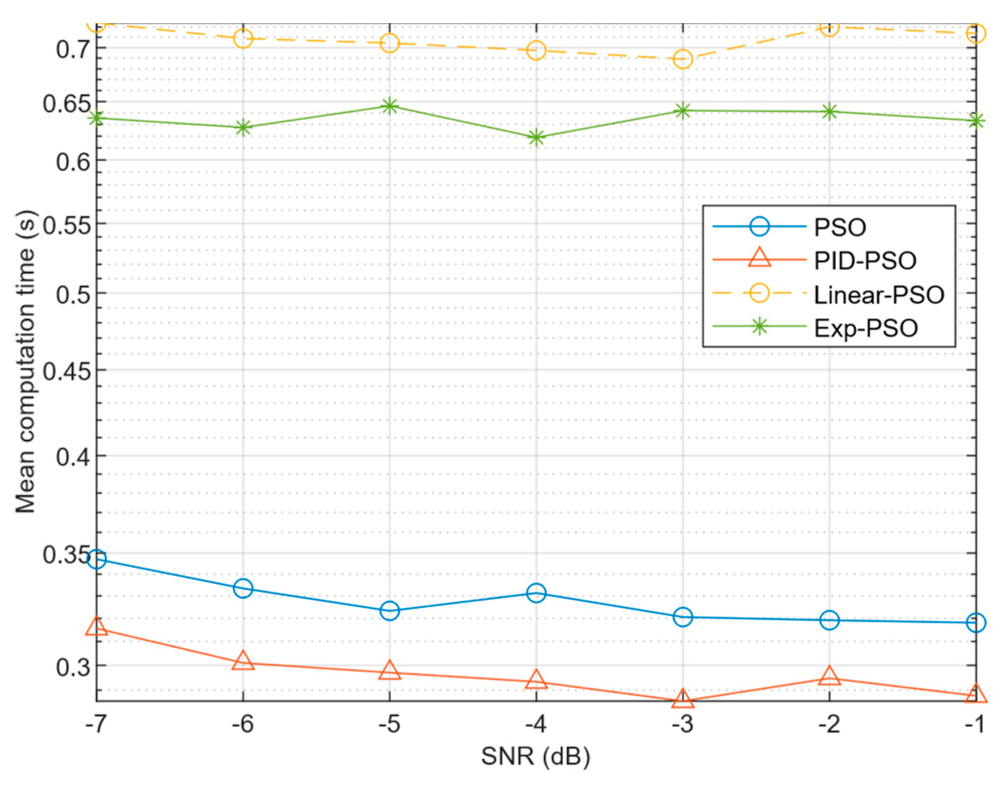
Assume the parameters of the LFM signal are A = 1 , f 0 = 10 , k = 30 , T = 2 , and the number of sampling points N = 512 . The SNR = { 7 , 6 , 5 , 4 , 3 , 2 , 1 } . The other experimental parameters are the same as those in Experiment 1. A comparison of the mean computation time between the basic PSO algorithm and the proposed PID-PSO algorithm, as well as two other improved PSO variants (Linear-PSO and Exp-PSO), is illustrated in Figure 12.
The mean iteration counts for convergence under different SNR levels are listed in Table 3.
The speed-up ratio results under different SNRs are shown in Table 4.
From Table 3 and Table 4 and Figure 10, the following patterns can be observed: The mean iteration count of the basic PSO algorithm fluctuates between 8.0610 and 8.7500 iterations, showing a significant increasing trend as the noise level rises. In contrast, the mean iteration count of the PID-PSO algorithm ranges from 7.2460 to 7.9620 iterations, consistently lower than that of the basic PSO algorithm across the entire SNR range, with stable fluctuations. The lowest speed-up ratio occurs at SNR = −2 dB, with a 7.95% improvement, while the most significant speed-up is observed at SNR = −4 dB, reaching 11.08%. Meanwhile, the search counts and computation time of Linear-PSO and Exp-PSO are substantially higher than those of Basic-PSO and PID-PSO. This indicates that PID-PSO can more efficiently accomplish the search for the optimal FRFT order and the parameter estimation of LFM signals.
From the algorithmic perspective: The basic PSO, due to its fixed inertia weight and non-adaptive step size, tends to oscillate or conduct redundant searches when approaching the optimal solution. In contrast, PID-PSO, through its proportional term adjusting direction, integral term promoting convergence, and derivative term suppressing oscillation, achieves a search strategy of “fast initially and stable later,” thus reaching the fitness threshold with fewer iterations. The analysis above is further supported by the results of the average computation time shown in Figure 12. Since the PID-PSO algorithm requires fewer iterations, its overall computation time is also significantly lower than that of the basic PSO algorithm.

3.3. Experiment 3: Sensitivity Analysis of PID Control Parameters for the Proposed PID-PSO-FRFT Algorithm

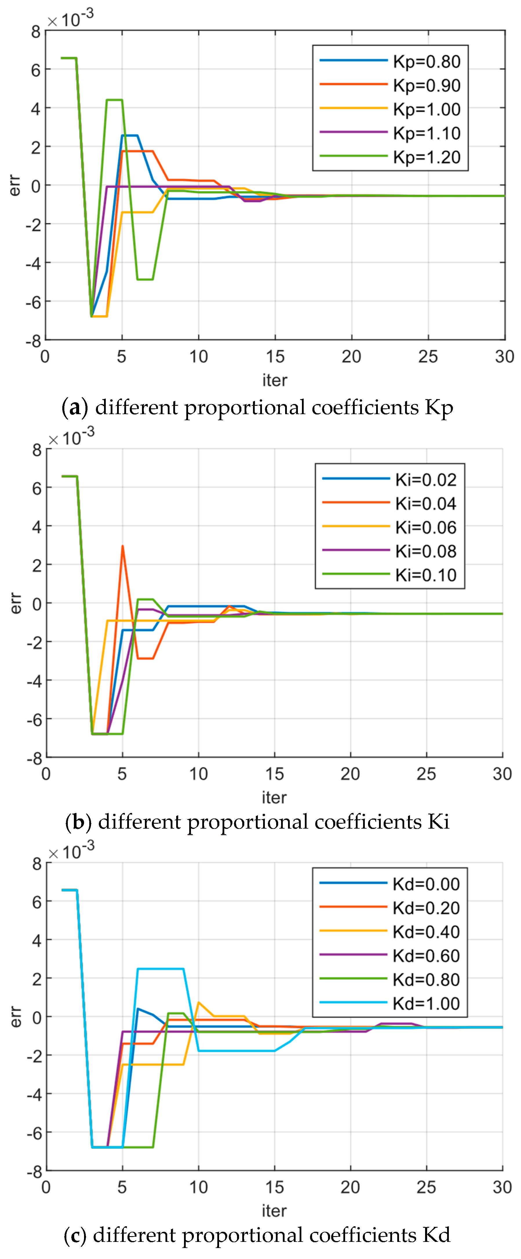
To investigate the influence of proportional, integral, and differential coefficients on the convergence performance of FRFT optimal order search, this section conducts a single-variable sensitivity analysis. The test uses an ideal noiseless LFM signal (f0 = 10, k = 30). All PSO parameters are kept consistent with Experiment 1, with only one PID coefficient adjusted each time and the other two fixed at the reference values (Kp = 1.0, Ki = 0.02, Kd = 0.2). The estimation deviation error, defined as the difference between the theoretical optimal FRFT order and the algorithm’s current global optimal value at each iteration, is used to characterize convergence speed, overshoot, and steady-state accuracy. The iterative variation curves of error under different PID parameters are shown in Figure 13.
From the iterative error variation curves in Figure 13, it can be observed that the proportional coefficient Kp, integral coefficient Ki, and differential coefficient Kd of the PID controller exert a significant and differentiated regulatory effect on the convergence dynamics of the algorithm during the FRFT optimal order search. However, they do not have a significant impact on the algorithm’s final convergence result. Specifically, the proportional coefficient Kp primarily governs the convergence speed in the early stages of the iteration: a smaller Kp results in a slower decline in the estimation error and a more gradual convergence, while a larger Kp accelerates convergence but may introduce more pronounced overshoot and oscillations. The integral coefficient Ki mainly influences the efficiency of steady-state error elimination: a smaller Ki leads to slower convergence of the residual steady-state error, whereas a larger Ki can easily induce persistent fluctuations during the iteration process. The differential coefficient Kd is primarily responsible for suppressing overshoot: a smaller Kd tends to cause more severe overshoot in the early stages, while a larger Kd effectively suppresses overshoot but may slightly slow down the convergence rate. It should be noted that the actual iterative characteristics depicted in the figure deviate to some extent from the ideal control behavior of a classic PID controller. This discrepancy is primarily attributed to the superimposed influence of the swarm intelligence characteristics inherent in the PSO algorithm itself, such as its nonlinear iteration process and stochastic particle updates.
Regarding the final convergence outcome, within the parameter range tested in this paper, irrespective of how the three PID coefficients were adjusted, the algorithm consistently and stably converged near the theoretical optimal FRFT order after 20 iterations, with the estimation error converging to a level approaching zero. This indicates that the adjustment of PID parameters primarily modifies the convergence dynamics of the algorithm without compromising its ultimate optimization efficacy. The algorithm thus demonstrates a wide range of adaptable PID parameters.

4. Conclusions

This paper applies an improved Particle Swarm Optimization (PSO) algorithm, which dynamically adjusts the inertia weight based on a Proportional-Integral-Derivative (PID) control strategy, to the search for the optimal order of the Fractional Fourier Transform (FRFT). This aims to enhance the parameter estimation accuracy of LFM signals using FRFT. The proposed adaptive method effectively addresses the issues of premature convergence and entrapment in local optima, which are common in traditional PSO algorithms due to a fixed inertia weight. Its core mechanism involves processing the deviation (and its change) between a particle’s current position and the global best position through three components: Proportional (P), Integral (I), and Derivative (D).
The proportional component provides a fundamental correction based on the magnitude of the real-time deviation: a larger deviation leads to a greater adjustment of the inertia weight, thereby driving particles rapidly toward the global optimal region. However, relying solely on proportional control can easily cause oscillations (“overshoot”) near the optimal solution and struggles to eliminate steady-state error entirely. The integral component overcomes this limitation by accumulating historical deviations. Particularly in later iterations, as the deviation decreases and the proportional effect weakens, the integral term continues to provide fine correction, gradually eliminating the steady-state error left by the proportional component, ensuring precise convergence of particles to the theoretical optimum. The derivative component performs anticipatory regulation based on the trend of deviation change. When a particle rapidly approaches the optimal solution (negative rate of change with a large absolute value), the derivative output provides a counteracting signal, effectively reducing particle velocity to prevent “overshoot” and oscillation caused by inertia. When the search stabilizes, its influence diminishes to avoid interfering with local fine-tuning.
Experiments and analysis demonstrate that, compared to the baseline PSO algorithm with a fixed linear decreasing and exponential decreasing inertia weight, the proposed method achieves higher convergence accuracy and stability in estimating the optimal FRFT order. When SNR < −7 dB, the basic PSO-FRFT algorithm quickly fails, whereas the PID-PSO-FRFT algorithm maintains parameter estimation accuracy until SNR < −9 dB, at which point the accuracy of PID-PSO-FRFT begins to degrade; meanwhile, although the Linear-PSO-FRFT and Exp-PSO-FRFT algorithms demonstrate a marginal improvement over the Basic-PSO-FRFT, they still fail to maintain high estimation accuracy, exhibiting performance degradation. Simultaneously, under SNR conditions within [−7 dB, −1 dB], the estimation speed of the PID-PSO-FRFT algorithm is consistently and significantly faster than that of the basic-PSO-FRFT, Linear-PSO-FRFT, and Exp-PSO-FRFT algorithms. Therefore, it is evident that PID-PSO-FRFT possesses better noise immunity, robustness, and faster estimation speed, also validating the theoretical analysis of improving the PSO algorithm using PID control strategies.
Future research could further explore extending the PID parameter control strategy to other parameters of the PSO algorithm (e.g., individual and social learning factors) to construct a more comprehensive multi-parameter collaborative optimization framework for FRFT.

Author Contributions

Conceptualization, X.L., C.W. and T.Z.; Methodology, X.L. and T.Z.; Software, T.Z.; Validation, X.L., T.Z. and B.X.; Formal Analysis, X.L. and T.Z.; Investigation, X.L., T.Z. and Y.C.; Resources, B.X. and C.W.; Data Curation, T.Z. and Y.W.; Writing—Original Draft, T.Z. and Y.W.; Writing—Review and Editing, T.Z., B.X., Y.W. and Y.C.; Visualization, T.Z., Y.W. and Y.C.; Supervision, X.L. and C.W.; Project Administration, X.L. and C.W.; Funding Acquisition, X.L. and C.W. All authors have read and agreed to the published version of the manuscript.

Funding

This research was funded by the National Natural Science Foundation of China (Grant 52402410).

Data Availability Statement

Data underlying the results presented in the paper can be obtained from the authors upon reasonable request. The code can be obtained from the corresponding author upon reasonable request.

Conflicts of Interest

The authors declare that they have no known competing financial interests or personal relationships that could have appeared to influence the work reported in this paper.

References

  1. Zhu, W.T.; Su, T.; Yang, T.; Zheng, J.B.; Zhu, K.R. Parameter estimation of linear frequency modulated continuous wave signals under low signal-to-noise ratio. Chin. J. Radio Sci. 2013, 28, 1158–1164. [Google Scholar] [CrossRef]
  2. Stove, A.G. Linear FMCW radar techniques. IEE Proc. F Radar Signal Process. 1992, 139, 343–350. [Google Scholar] [CrossRef] [Scilit]
  3. Shi, C.; Wang, F.; Salous, S.; Zhou, J. Low probability of intercept-based radar waveform design for distributed multiple-radar systems. Entropy 2018, 20, 197. [Google Scholar] [CrossRef] [Scilit]
  4. Mao, Y.T. Generalized Linear Frequency-Domain Chirplet Transform and Its Application. Pure Math. 2024, 14, 642–648. [Google Scholar] [CrossRef]
  5. Zhou, Y.X.; Ma, Z.P.; Fu, L. A Review of Key Signal Processing Techniques for Structural Health Monitoring: Highlighting Non-Parametric Time-Frequency Analysis, Adaptive Decomposition, and Deconvolution. Algorithms 2025, 18, 318. [Google Scholar] [CrossRef] [Scilit]
  6. Morlet, J.; Arens, G.; Fourgeau, E.; Giard, D. Wave propagation and sampling theory—Part I: Complex signal and scattering in multilayered media. Geophysics 2012, 47, 203–221. [Google Scholar] [CrossRef] [Scilit]
  7. Mateo, C.; Talavera, A.J. Bridging the gap between the short-time Fourier transform (STFT), wavelets, the constant-Q transform and multi-resolution STFT. Signal Image Video Process. 2020, 14, 1535–1543. [Google Scholar] [CrossRef] [Scilit]
  8. Li, M.Y.; Chen, W.Z.; Zhang, T. Automatic epileptic EEG detection using DT-CWT-based non-linear features. Biomed. Signal Process. Control. 2017, 34, 114–125. [Google Scholar] [CrossRef] [Scilit]
  9. Sarna, M.; Hossian, M.R.; Islam, M.A. Comparative analysis of STFT and wavelet transform in time-frequency analysis of non-stationary signals. Nov. Trends Comput. 2024, 1, 72–78. [Google Scholar] [CrossRef]
  10. Huang, D.Z.; Han, L.G.; Li, H.F.; Yang, F.; Zhao, X.; Sun, N. Separation of multi-source seismic data based on S-transform adaptive filtering iteration. Pet. Geophys. Prospect. 2020, 55, 1253–1262. [Google Scholar] [CrossRef]
  11. Stockwell, R.G.; Mansinha, L.; Lowe, R.P. Localization of the complex spectrum: The S transform. IEEE Trans. Signal Process. 1996, 44, 998–1001. [Google Scholar] [CrossRef] [Scilit]
  12. Beuter, C.; Oleskovicz, M. S-transform: From main concepts to some power quality applications. IET Signal Process. 2020, 14, 115–123. [Google Scholar] [CrossRef] [Scilit]
  13. Wu, G.N.; Cao, S.Y.; Ma, N. Time-frequency analysis characteristics of the S-transform and its improvement. Prog. Geophys. 2011, 26, 1661–1667. [Google Scholar]
  14. Satyanarayana, V.V.S.; Krishna, M.B.; Satyanarayana, V.V.P.; Kumari, E.K. Reduction of Interference Terms in Wigner Ville Distribution using Machine Learning. Circuits Syst. Signal Process. 2024, 44, 2041–2072. [Google Scholar] [CrossRef] [Scilit]
  15. Zou, Y.; Li, X.; Yu, G. Adaptive WVD Cross-Term Removal Method Based on Multidimensional Property Differences. J. Mar. Sci. Appl. 2024, 24, 774–788. [Google Scholar] [CrossRef] [Scilit]
  16. Shekhar, C.; Raj, B.A.A. Time-optimised real-time time–frequency measurement technique for RoFSO applications. Measurement 2025, 253, 117698. [Google Scholar] [CrossRef] [Scilit]
  17. Ristic, B.; Boashash, B. Use of the cross polynomial Wigner-Ville distribution for instantaneous frequency estimation of nonlinear FM signals. In Proceedings of the IEEE-SP International Symposium on Time-Frequency and Time-Scale Analysis, Philadelphia, PA, USA, 25-28 October 1994; IEEE: Victoria, BC, Canada, 1994; pp. 252–255. [Google Scholar] [CrossRef] [Scilit]
  18. Lu, L.; Ren, W.X.; Wang, S.D. Fractional Fourier transform: Time-frequency representation and structural instantaneous frequency identification. Mech. Syst. Signal Process. 2022, 178, 109305. [Google Scholar] [CrossRef] [Scilit]
  19. Aldmashke, O.; Serbes, A. LFM signal parameter estimation in the fractional Fourier domains: Analytical models and a high-performance algorithm. Signal Process. 2024, 214, 109224. [Google Scholar] [CrossRef] [Scilit]
  20. Lu, Z.K.; Liu, S.H.; Qiu, J.; Huang, Q.; Yang, C. An efficient method for parameter estimation and separation of multi-component LFM signals. Signal Process. 2023, 207, 108964. [Google Scholar] [CrossRef] [Scilit]
  21. Xuelian, L.; Xiao, B.; Wang, C. Optimal target function for the fractional Fourier transform of LFM signals. Circuits Syst. Signal Process. 2022, 41, 4160–4173. [Google Scholar] [CrossRef] [Scilit]
  22. Xuelian, L.; Xiao, B.; Wang, C. Frequency estimation of chirp signals based on fractional fourier transform combined with Otsu’s method. Optik 2021, 240, 166945. [Google Scholar] [CrossRef] [Scilit]
  23. Yan, B.M.; Li, Y.; Cheng, W. High-resolution multicomponent LFM parameter estimation based on deep learning. Signal Process. 2025, 227, 109714. [Google Scholar] [CrossRef] [Scilit]
  24. Shen, L.; Yin, Q.; Lu, M.; Zhang, Q.; Guo, L.; Shen, T.; Zhao, G.; Ning, S. Linear FM Signal Parameter Estimation Using STFT and FRFT. Chin. J. Electron. 2013, 22, 301–307. [Google Scholar]
  25. Liu, X. Parameter estimation of LFM signal intercepted by Nyquist folding receiver based on particle swarm optimization and fractional Fourier transform. In Proceedings of the International Conference on Computer Application and Information Security (ICCAIS 2024), Wuhan, China, 20-22 December 2024; SPIE: Bellingham, WA, USA, 2025; Volume 13562, pp. 212–219. [Google Scholar] [CrossRef] [Scilit]
  26. Wang, H.; Guo, Y.; Yang, L. Parameter estimation of LFM signals based on FOTD-CFRFT under impulsive noise. Fractal Fract. 2023, 7, 822. [Google Scholar] [CrossRef] [Scilit]
  27. Guo, Y.; Yang, L. Method for parameter estimation of LFM signal and its application. IET Signal Process. 2019, 13, 538–543. [Google Scholar] [CrossRef] [Scilit]
  28. Kennedy, J.; Eberhart, R.C. Particle swarm optimization. In Proceedings of the ICNN’95—International Conference on Neural Networks, Perth, Australia, 27 November–1 December 1995; IEEE: New York, NY, USA, 1995; pp. 1942–1948. [Google Scholar] [CrossRef] [Scilit]
  29. Han, Y.; Lin, M.; Li, N.; Qi, Q.; Li, J.; Liu, Q. DCWPSO: Particle swarm optimization with dynamic inertia weight updating and enhanced learning strategies. PeerJ Comput. Sci. 2024, 10, e2253. [Google Scholar] [CrossRef] [Scilit]
  30. Sameh, K.; Dominique, B. Particle Swarm Optimization with Adaptive Inertia Weight. Int. J. Mach. Learn. Comput. 2015, 5, 368–373. [Google Scholar] [CrossRef] [Scilit]
  31. Saxena, S.; Pohit, M. A new non linear inertia weight approach in PSO for faster rigid image registration. In Proceedings of the 2019 6th International Conference on Signal Processing and Integrated Networks (SPIN), Noida, India, 7–8 March 2019; IEEE: New York, NY, USA, 2019; pp. 607–612. [Google Scholar] [CrossRef] [Scilit]
  32. Ratnawati, D.E.; Marjono, M.; Widodo, W.; Anam, S. PSO-ELM with time-varying inertia weight for classification of SMILES codes. Int. J. Intell. Eng. Syst. 2020, 18, 2146–2155. [Google Scholar] [CrossRef] [Scilit]
  33. Huang, C.; Zhao, Y.; Zhang, M.; Yang, H. APSO: An A*-PSO Hybrid Algorithm for Mobile Robot Path Planning. IEEE Access 2023, 11, 43248–43263. [Google Scholar] [CrossRef] [Scilit]
  34. Bharti, K.K.; Singh, K.P. Opposition chaotic fitness mutation based adaptive inertia weight BPSO for feature selection in text clustering. Appl. Soft Comput. 2016, 43, 20–34. [Google Scholar] [CrossRef] [Scilit]
  35. Zaineb, A.; Kamel, B. Fractional Fourier Transform, Signal Processing and Uncertainty Principles. Circuits Syst. Signal Process. 2022, 42, 892–912. [Google Scholar] [CrossRef] [Scilit]
  36. Chunyang, W.; Xuelian, L. Application of fractional Fourier transform in signal processing. J. Chang. Univ. Sci. Technol. (Nat. Sci. Ed.) 2015, 38, 1–8. [Google Scholar]
  37. Liu, X.; Han, J.; Wang, C.; Xiao, B. Parameter estimation of linear frequency modulation signals based on sampling theorem and fractional broadening. Rev. Sci. Instrum. 2019, 90, 014702. [Google Scholar] [CrossRef] [Scilit] [PubMed]
  38. Ozaktas, H.M.; Arikan, O.; Kutay, M.A.; Bozdagt, G. Digital computation of the fractional Fourier transform. IEEE Trans. Signal Process. 1996, 44, 2141–2150. [Google Scholar] [CrossRef] [Scilit]
  39. Zhao, X.H.; Deng, B.; Tao, R. Dimensional normalization in numerical computation of fractional Fourier transform. J. Beijing Inst. Technol. 2005, 25, 360–364. [Google Scholar] [CrossRef]
  40. Guan, J.; Jiang, X.Y.; Liu, N.B.; Ding, H.; Dong, Y.; Liu, T. Enhanced target detection using fractional Fourier transform features with threshold-modified normalization. Electron. Lett. 2024, 60, e13252. [Google Scholar] [CrossRef] [Scilit]
Figure 1. Schematic diagram of the LFM signal.
Fractalfract 10 00202 g001aFractalfract 10 00202 g001b
Figure 2. Schematic diagram of coordinate axis rotation.
Fractalfract 10 00202 g002
Figure 3. Energy Concentration of FRFT.
Fractalfract 10 00202 g003
Figure 4. Flowchart of the Adopted Discrete FRFT Algorithm.
Fractalfract 10 00202 g004
Figure 5. Flowchart of FRFT-based LFM Parameter Estimation.
Fractalfract 10 00202 g005
Figure 6. Flowchart of the PSO Algorithm.
Fractalfract 10 00202 g006
Figure 7. Flowchart of the PID-PSO-FRFT Algorithm.
Fractalfract 10 00202 g007
Figure 8. RMSE Curves of Parameter Estimation under Different Algorithms versus SNR (LFM: f0 = 70, k = 60).
Fractalfract 10 00202 g008
Figure 9. RMSE Curves of Parameter Estimation under Different Algorithms versus SNR (LFM: f0 = 10, k = 30).
Fractalfract 10 00202 g009
Figure 10. Variance of estimated f0 and k under different SNRs (LFM: f0 = 70, k = 60).
Fractalfract 10 00202 g010
Figure 12. Comparison of Mean Parameter Estimation Time under Different SNRs.
Fractalfract 10 00202 g012
Figure 13. Iterative variation curves of FRFT optimal order estimation deviation under different PID control parameters.
Fractalfract 10 00202 g013
Table 1. Parameter Settings of the Search Algorithms.
Algorithm ParameterParameter Value
Learning Factor c11.4962
Learning Factor c20.9
Maximum Iterations50
Search Dimension1
Population Size50
Initial PositionRandomly selected within the bounds
Initial v of PSORandomly selected within the bounds
Search Range[0.7, 1.3]
v of Range[−0.6, 0.6]
Table 2. Inertia Weight ω and Additional Tuning Parameter Settings.
AlgorithmInertia Weight ω SettingAdditional Tuning Parameters
Basic PSOω = 0.7\
PID-PSOInitial ω = 0.7, ω ∈ [0.4, 1.4]P = 1; I = 0.02; D = 0.2.
Linear-PSOInitial ω = 0.7, ω ∈ [0.4, 1.4]\
Exp-PSOInitial ω = 0.7, ω ∈ [0.4, 1.4]\
Table 3. Mean Iteration Counts from 1000 Repeated Experiments.
SNR (dB)−7−6−5−4−3−2−1
Mean Iteration CountBasic PSO8.75008.41908.21808.37008.13708.06108.0620
Linear-PSO18.339017.992017.897017. 715017.538018.234018.1470
Exp-PSO16.132015.893016.394015.734016.323016.198016.1020
PID-PSO7.96207.61407.53207.44207.24607.42007.2970
Table 4. Speed-up Ratio Results under Different SNRs.
SNR (dB)−7−6−5−4−3−2−1
Speed-up Ratio (%)9.009.568.3511.0910.957.959.49
Disclaimer/Publisher’s Note: The statements, opinions and data contained in all publications are solely those of the individual author(s) and contributor(s) and not of MDPI and/or the editor(s). MDPI and/or the editor(s) disclaim responsibility for any injury to people or property resulting from any ideas, methods, instructions or products referred to in the content.