Fractional Calculus of Fractal Functions on Weighted Sobolev Spaces

Abstract

In this article, the $\alpha$-fractal interpolation function $f^{\alpha }$ corresponding to any function f belonging to the weighted Sobolev space ${\mathcal{W}}_{\rho }^{r,2}\left(I\right)$ is defined. The convergence of sequences of $\alpha$-fractal interpolation functions corresponding to mappings in ${\mathcal{W}}_{\rho }^{r,2}\left(I\right)$ with respect to the uniform norm as well as the weighted Sobolev norm is discussed. It is proved that the Riemann–Liouville fractional order integral of an $\alpha$-fractal interpolation function of any map $f\in {\mathcal{W}}_{\rho }^{r,2}\left(I\right)$ is also a self-referential function interpolating a specific data set. Some aspects of the convergence of the Riemann–Liouville integral of $\alpha$-fractal functions when the original mappings converge are also analyzed. In short, by imposing certain conditions on the base function and the scale vector of a specific iterated function system, fractal perturbations of functions from weighted Sobolev spaces are defined. It is also proved that, under suitable hypotheses, the Riemann–Liouville fractional integral of these fractal mappings on Sobolev spaces is a fractal function of the same kind.

1. Introduction

Fractal analysis is a new mathematical tool helping to understand complexities and irregularities in nature. In particular, fractal interpolation is a conventional way to approximate nonlinear data obtained from scientific experiments or social phenomena. Deterministic fractal maps defined through specific iterated function systems (IFSs) are appropriate examples of continuous and nowhere differentiable functions, and the fractional calculus is a suitable mathematical operator for analyzing and applying such maps.

The notion of fractal interpolation function (FIF) was introduced by M.F. Barnsley [1]. The author [1,2] constructed a FIF based on an IFS so that the attractor of the IFS is the graph of a continuous function which interpolates a given data set. Moreover, the FIF is also described as the unique fixed point of the well known contraction Read–Bajraktarević (RB) operator defined on $\mathcal{C}\left(I\right)$, the space of all continuous real-valued functions defined on a compact interval I of $\mathbb{R}$. Later, Navascués [3] developed the theory of FIF and introduced the concept of $\alpha$-fractal (interpolation) function $f^{\alpha }$ as a fractal perturbation of a function $f\in \mathcal{C}\left(I\right)$. Several discussions on the properties of an $\alpha$-FIF and its applications can be found in the abundant literature on the topic (see, for instance, [4]). The function $f^{\alpha }$ may be continuous but in general nowhere differentiable.

Barnsley et al. [5] introduced the calculus of FIFs and proved that integration of a FIF is also a FIF. Navascués et al. [6] presented a technique for the numerical integration of an affine fractal function. Additionally, an upper bound of the error committed in the numerical process was estimated. In [7], the continuity of the Riemann–Liouville fractional order integral of a FIF is discussed and it is shown that FIFs can be integrated on any closed interval $[a,b]\subset [0,\infty )$. In the same article, it was also proved that the fractional order integral of a FIF remains a FIF on the interval $[0,b](b>0)$. In [8], the classical integral of various types of FIFs was investigated. Ruan et al. [9] proved that the fractional integral of a linear FIF remains a linear FIF and, in certain instances, established a linear connection between the order of the fractional integral and the box dimension of two affine FIFs. In [10], the properties of the fractional order calculus of FIFs generated by affine iterated function systems were studied and shown that the fractional order integral of such FIFs is continuous and differentiable on the closed interval $[0,b](b>0)$. In [11], it is shown that the Riemann–Liouville fractional integral of an $\alpha$-fractal function $f^{\alpha }$ is also an $\alpha$-fractal function of a new set of data points associated with a suitable IFS. The Riemann–Liouville fractional calculus of coalescence hidden-variable fractal interpolation function is studied in [12]. In [13], the R-fractal interpolation function was introduced, and the results proving the existence of differentiable and smooth FIFs with any order of regularity were extended to R-fractal interpolation functions.

In most cases, the experimental, social and scientific data structures are intricate and irregular, and they are not well fitted by the classical spaces of smooth functions. In this context, our work establishes a better model in the framework of fractal functions in functional spaces like the weighted Sobolev spaces, allowing the modeling of complex phenomena, where the standard mild and local characteristics do not hold. By the use of weights, Sobolev spaces capture local irregularities that can be related to fractal measures and norms. The weights also enable the study of functions in the neighborhoods of singular points or domains with a great complexity, that can be well fitted by fractal and fractional structures. Some recent articles on this topic are, for instance, references [14,15,16].

This paper complements some results given in reference [17] for fractal functions belonging to unweighted Sobolev spaces, considering a different norm. It also studies fractional integral operators of the Riemann–Liouville type acting on $\alpha$-fractal functions. Section 2 presents some useful definitions and notations needed in the article. In Section 3, the fractal analogue $f^{\alpha }$ of any function f belonging to the weighted Sobolev space ${\mathcal{W}}_{\rho }^{r,2}\left(I\right)$ is defined. Some results on the convergence of sequences of $\alpha$-fractal functions are established in Section 4. In Section 5, it is shown that the Riemann–Liouville fractional order integral $I_{x_0}^{\nu }{f}^{\alpha }$ of an $\alpha$-fractal function $f^{\alpha }$ corresponding to $f\in {\mathcal{W}}_{\rho }^{r,2}\left(I\right)$ is also a self-referential function interpolating a set of points lying on the fractional order integral $I_{x_0}^{\nu }f$ of f, as $f^{\alpha }$ interpolates the points that lie on f. Moreover, some aspects of the convergence of a sequence ${\left\{I_{x_0}^{\nu }{f}_n^{\alpha }\right\}}_{n=1}^{\infty }$ of such fractional order integrals of $\alpha$-fractal functions with respect to different norms are discussed.

2. Preliminaries

2.1. Fractal Interpolation Function

Let $N\ge 2$ be any integer. Consider a set of interpolation points $\{(x_i,y_i)\in I\times \mathbb{R}:i=0,1,\dots ,N\}$, where $\Delta :x_0<x_1<\cdots <x_N$ is a partition of the interval $I=[x_0,x_N]$ of $\mathbb{R}$. Let $J=\{1,2,\dots ,N\}$. Set $I_i=[x_{i-1},x_i]$, $i\in J$. For $i\in J$, let $L_i:I\to I_i$, be contractive homeomorphisms satisfying the join-up conditions

$$L_i\left(x_0\right)=x_{i-1},L_i\left(x_N\right)=x_i.$$

Also, consider N continuous mappings $F_i:I\times \mathbb{R}\to \mathbb{R}$ such that

$$F_i(x_0,y_0)=y_{i-1},F_i(x_N,y_N)=y_i,$$

(1)

$$\left|F_i(x,y)-F_i(x,y^{\prime })\right|\le \left|{\alpha }_i\right|\left|y-y^{\prime }\right|,$$

(2)

for all x in I and for all $y,y^{\prime }$ in $\mathbb{R}$ and for some $0\le \left|{\alpha }_i\right|<1,i\in J$. Consider the IFS $W=\{I\times \mathbb{R};w_i(x,y):i\in J\}$, where the mappings $w_i:I\times \mathbb{R}\to I_i\times \mathbb{R}$ are given by

$$w_i(x,y)=(L_i\left(x\right),F_i(x,y)).$$

(3)

In general, the unique nonempty compact subset $G\in I\times \mathbb{R}$ which satisfies the invariance equation $G={\bigcup }_{i=1}^N{w}_i\left(G\right)$ is called attractor of the IFS W.

With the described choice of $L_i$ and $F_i$, the attractor G is the graph of a continuous function $g:I\to \mathbb{R}$ which obeys $g\left(x_i\right)=y_i$ for $i\in J$ [2]. The function g is the fractal interpolation function (FIF) corresponding to the IFS (3).

Let ${\mathcal{C}}^{*}\left(I\right)=\{f\in \mathcal{C}\left(I\right):f\left(x_0\right)=y_0,f\left(x_N\right)=y_N\}$ and ${\mathcal{C}}^{**}\left(I\right)=\{f\in \mathcal{C}\left(I\right):f\left(x_i\right)=y_i$; $i=0,1,2,\dots ,N\}$. The FIF g is also the fixed point of the Read–Bajraktarevic (RB) operator $T:{\mathcal{C}}^{*}\left(I\right)\to {\mathcal{C}}^{**}\left(I\right)$ defined by (see [18])

$$\left(Tf\right)\left(x\right)=F_i(L_i^{-1}\left(x\right),f\left(L_i^{-1}\left(x\right)\right));x\in I_i,i\in J.$$

It is well known that T is a contraction with contractivity factor ${\left|\alpha \right|}_{\infty }=max\{\left|{\alpha }_i\right|:i\in J\}<1$. The unique fixed point of T is the FIF g corresponding to the IFS (3) and consequently it is the unique function satisfying the self-referential equation:

$$g\left(x\right)=F_i(L_i^{-1}\left(x\right),g\left(L_i^{-1}\left(x\right)\right));x\in I_i,i\in J.$$

(4)

For each $i\in J$, ${\alpha }_i$ is a parameter restricted by the condition $\left|{\alpha }_i\right|<1$ and is called a vertical scaling factor of $w_i$. The corresponding vector $\alpha =({\alpha }_1,{\alpha }_2,\dots ,{\alpha }_N)$ is called the scale vector of the IFS (3).

A widely used class of FIF is defined by the mappings

$$L_i\left(x\right)=a_{i}x+e_i,F_i(x,y)={\alpha }_{i}y+v_i\left(x\right),$$

where $a_i={\displaystyle \frac{x_i-x_{i-1}}{x_N-x_0}}$, $e_i={\displaystyle \frac{x_N{x}_{i-1}-x_0{x}_i}{x_N-x_0}}$, and $v_i\left(x\right)$ are suitable continuous functions such that conditions (1) and (2) are satisfied. If $v_i\left(x\right)$ are linear, then the corresponding FIF is known as affine FIF.

2.2. $\alpha$-Fractal Interpolation Function

Definition 1.

For a continuous function $f\in \mathcal{C}\left(I\right)$, the α-fractal interpolation function (or simply α-fractal function) $f^{\alpha }$ is the FIF when we consider the IFS defined by the following mappings [3]:

$$L_i\left(x\right)=a_{i}x+e_i,$$

$$F_i(x,y)={\alpha }_{i}y+f\left(L_i\left(x\right)\right)-{\alpha }_{i}b\left(x\right),$$

where $a_i={\displaystyle \frac{x_i-x_{i-1}}{x_N-x_0}}$, $e_i={\displaystyle \frac{x_N{x}_{i-1}-x_0{x}_i}{x_N-x_0}};$$b\in \mathcal{C}\left(I\right)$ is a continuous function satisfying the conditions $b\left(x_0\right)=f\left(x_0\right)$, $b\left(x_N\right)=f\left(x_N\right)$ and $\left|{\alpha }_i\right|<1,i\in J$. Map b is usually known as base function.

For an $\alpha$-fractal function $f^{\alpha }$ modeling a signal, map f provides the trend of the record and map b modulates the small self-affine oscillations around it, whose amplitude depends on the size of the vector $\alpha$. In general, greater vectors $\alpha$ produce more complex graphs for $f^{\alpha }$.

From (4), the $\alpha$-fractal function $f^{\alpha }$ satisfies the self-referential equation

$$f^{\alpha }\left(x\right)=f\left(x\right)+{\alpha }_i(f^{\alpha }-b)\left(L_i^{-1}\left(x\right)\right),$$

(5)

for all $x\in I_i,$$i\in J$. From (5), it is easy to deduce that

$${∥f^{\alpha }-f∥}_{\infty }\le {\displaystyle \frac{{\left|\alpha \right|}_{\infty }}{1-{\left|\alpha \right|}_{\infty }}}{∥f-b∥}_{\infty }.$$

For $\alpha =0$, the fractal function $f^{\alpha }$ agrees with f. The operator ${\mathcal{F}}^{\alpha }:\mathcal{C}\left(I\right)\to \mathcal{C}\left(I\right)$ defined by

$${\mathcal{F}}^{\alpha }\left(f\right)=f^{\alpha }\mathrm{for}\mathrm{all}f\in \mathcal{C}\left(I\right)$$

is linear and bounded for various choices of b (see [3]).

Let $b=Lf$, where $L:\mathcal{C}\left(I\right)\to \mathcal{C}\left(I\right)$ is a linear and bounded operator with respect to the uniform norm on $\mathcal{C}\left(I\right)$ such that $Lf\left(x_0\right)=f\left(x_0\right)$ and $Lf\left(x_N\right)=f\left(x_N\right)$. Then, for any $f\in \mathcal{C}\left(I\right),$ its fractal function $f^{\alpha }$ satisfies [4]

$${∥f^{\alpha }-f∥}_{\infty }\le {\left|\alpha \right|}_{\infty }{∥f^{\alpha }-Lf∥}_{\infty }$$

and

$${∥f^{\alpha }-f∥}_{\infty }\le {\displaystyle \frac{{\left|\alpha \right|}_{\infty }}{1-{\left|\alpha \right|}_{\infty }}}{∥Id-L∥}_{\infty }{∥f∥}_{\infty },$$

where $Id$ denotes the identity and ${∥Id-L∥}_{\infty }$ represents the corresponding operator norm.

2.3. Weighted ${\mathcal{L}}^p$ and Weighted Sobolev Spaces

Roughly speaking, for $1\le p<\infty$, a weighted ${\mathcal{L}}^p$-space on the compact interval $I=[a,b]$ of $\mathbb{R}$ with a continuous weight $\rho :I\to (0,\infty )$ is defined as ${\mathcal{L}}_{\rho }^p\left(I\right):=\{f:I\to \mathbb{R};f$ is measurable and ${∥f∥}_{{\mathcal{L}}_{\rho }^p\left(I\right)}<\infty \}$, where

$${∥f∥}_{{\mathcal{L}}_{\rho }^p\left(I\right)}:={\left[{\int }_I{\left|f\left(x\right)\right|}^p\rho \left(x\right)dx\right]}^{{\displaystyle \frac{1}{p}}},1\le p<\infty .$$

For sup-norm and ${\mathcal{L}}_{\rho }^p$-norm, we have

$${∥f∥}_{{\mathcal{L}}_{\rho }^p\left(I\right)}\le {∥f∥}_{\infty }{\left[{\int }_I\rho \left(x\right)dx\right]}^{{\displaystyle \frac{1}{p}}},$$

where sup-norm ${∥f∥}_{\infty }=esssup\{\left|f\left(x\right)\right|:x\in I\}$ if f is essentially bounded.

Write ${\mathcal{L}}_{\rho }^p\left(I\right)={\mathcal{L}}^p\left(I\right)$ for $\rho \left(x\right)=1$ and ${\mathcal{L}}^1\left(I\right)=\mathcal{L}\left(I\right)$. If ${\displaystyle \frac{1}{\rho \left(x\right)}}\in \mathcal{L}\left(I\right)$, then Hölder’s inequality provides that ${\mathcal{L}}_{\rho }^2\left(I\right)\subset \mathcal{L}\left(I\right)$. Let us denote throughout the article ${\rho }_0=\underset{x\in I}{min}\rho \left(x\right),{\rho }_1=\underset{x\in I}{max}\rho \left(x\right)$.

Let r be any positive integer. The weighted Sobolev space [19] is defined as ${\mathcal{W}}_{\rho }^{r,2}\left(I\right):=\{f:I\to \mathbb{R};f$ is $(r-1)$-times continuously differentiable on I such that $f^{(r-1)}$ is absolutely continuous on I and $f^{\left(r\right)}\in {\mathcal{L}}_{\rho }^2\left(I\right)\}$.

The inner product in ${\mathcal{W}}_{\rho }^{r,2}\left(I\right)$ is defined as

$$〈f,g〉=\sum _{j=0}^{r-1}{f}^{\left(j\right)}\left(a\right)g^{\left(j\right)}\left(a\right)+{\int }_I{f}^{\left(r\right)}\left(x\right)g^{\left(r\right)}\left(x\right)\rho \left(x\right)dx,$$

(6)

for all $f,g\in {\mathcal{W}}_{\rho }^{r,2}\left(I\right)$ and the (weighted Sobolev) norm is defined as

$${∥f∥}_{{\mathcal{W}}_{\rho }^{r,2}\left(I\right)}={\left[\sum _{j=0}^{r-1}{\left|f^{\left(j\right)}\left(a\right)\right|}^2+{\int }_I{\left|f^{\left(r\right)}\left(x\right)\right|}^2\rho \left(x\right)dx\right]}^{{\displaystyle \frac{1}{2}}},$$

(7)

for all $f\in {\mathcal{W}}_{\rho }^{r,2}\left(I\right)$.

This makes ${\mathcal{W}}_{\rho }^{r,2}\left(I\right)$ a Hilbert space with respect to the inner product (6). From the definition it is clear that ${\mathcal{W}}_{\rho }^{r,2}\left(I\right)\subset \mathcal{C}\left(I\right)$. It is needed to mention that for any compact interval I, ${\mathcal{C}}^r\left(I\right)$, the space of all r-times continuously differentiable functions on I is dense in ${\mathcal{W}}_{\rho }^{r,2}\left(I\right)$ (in view of Theorem 2, Page 251 in [20]). We will call the functions from this Sobolev space Sobolev functions.

3. Fractal Functions on ${\mathcal{W}}_{\rho }^{\mathbf{r},\mathbf{2}}\left(\mathbf{I}\right)$

In the following theorem, $\alpha$-fractal functions on the weighted Sobolev space ${\mathcal{W}}_{\rho }^{r,2}\left(I\right)$ are defined and bounded with respect to the norm (7).

Theorem 1.

Let $f\in {\mathcal{W}}_{\rho }^{r,2}\left(I\right)$. Suppose that $\Delta :x_0<x_1<\cdots <x_N$ is a partition of the interval $I=[x_0,x_N]$. For $i\in J$, set $I_i=[x_{i-1},x_i]$ and let $L_i:I\to I_i$ be the maps $L_i\left(x\right)=a_{i}x+e_i$, satisfying $L_i\left(x_0\right)=x_{i-1}$, $L_i\left(x_N\right)=x_i$. Let the base function $b\in {\mathcal{W}}_{\rho }^{r,2}\left(I\right)$ and the scale vector $\alpha =({\alpha }_1,{\alpha }_2,\dots ,{\alpha }_N)\in {\mathbb{R}}^N$ satisfy

$$b^{\left(j\right)}\left(x_0\right)=f^{\left(j\right)}\left(x_0\right),b^{\left(j\right)}\left(x_N\right)=f^{\left(j\right)}\left(x_N\right)$$

(8)

for $j=1,2,\dots ,r-1,$

$$|{\alpha }_i|<a_i^{r-1},$$

(9)

for $i=1,2,\dots ,N$ and

$${\left[{\displaystyle \frac{{\rho }_1}{{\rho }_0}}\sum _{i=1}^N{\displaystyle \frac{{\left|{\alpha }_i\right|}^2}{a_i^{2r-1}}}\right]}^{{\displaystyle \frac{1}{2}}}<1.$$

(10)

Then the RB operator $T:{\mathcal{W}}_{\rho }^{r,2}\left(I\right)\to {\mathcal{W}}_{\rho }^{r,2}\left(I\right)$ defined by

$$\left(Tg\right)\left(x\right)=f\left(x\right)+{\alpha }_i(g-b)\left(L_i^{-1}\left(x\right)\right);x\in I_i,i\in J,$$

is a contraction on ${\mathcal{W}}_{\rho }^{r,2}\left(I\right)$ with respect to the norm (7). Furthermore, T has a unique fixed point (α -fractal function) $f^{\alpha }\in {\mathcal{W}}_{\rho }^{r,2}\left(I\right)$ that obeys the self-referential equation

$$f^{\alpha }\left(x\right)=f\left(x\right)+{\alpha }_i(f^{\alpha }-b)\left(L_i^{-1}\left(x\right)\right);x\in I_i,i\in J.$$

Proof. 

For any $g,h\in {\mathcal{W}}_{\rho }^{r,2}\left(I\right)$,

$$(Tg-Th)\left(x\right)={\alpha }_i(g-h)\left(L_i^{-1}\left(x\right)\right);x\in I_i,i\in J$$

(11)

and

$${∥Tg-Th∥}_{{\mathcal{W}}_{\rho }^{r,2}\left(I\right)}={\left[\begin{array}{c}\sum _{j=0}^{r-1}{\left|{(Tg-Th)}^{\left(j\right)}\left(x_0\right)\right|}^2\\ +{\int }_I{\left|{(Tg-Th)}^{\left(r\right)}\left(x\right)\right|}^2\rho \left(x\right)dx\end{array}\right]}^{{\displaystyle \frac{1}{2}}}.$$

(12)

For $j=0,1,2,\dots ,r$ and $x\in I_i,$$i\in J$, we have, from (11),

$${(Tg-Th)}^{\left(j\right)}\left(x\right)={\displaystyle \frac{{\alpha }_i}{a_i^j}}{(g-h)}^{\left(j\right)}\left(L_i^{-1}\left(x\right)\right)$$

(13)

As $x_0\in I_1$, from (13), for $j=0,1,2,\dots ,r$, we have

$${(Tg-Th)}^{\left(j\right)}\left(x_0\right)={\displaystyle \frac{{\alpha }_1}{a_1^j}}{(g-h)}^{\left(j\right)}\left(L_1^{-1}\left(x_0\right)\right).$$

(14)

Since $0<a_1<1$, then ${\displaystyle \frac{1}{a_1^{2j}}}\le {\displaystyle \frac{1}{a_1^{2(r-1)}}}$ for all $j=0,1,2,\dots ,(r-1)$ and consequently, using (14), we have

$$\begin{array}{ccc}\hfill \sum _{j=0}^{r-1}{\left|{(Tg-Th)}^{\left(j\right)}\left(x_0\right)\right|}^2& =& \sum _{j=0}^{r-1}{\displaystyle \frac{{\left|{\alpha }_1\right|}^2}{a_1^{2j}}}{\left|{(g-h)}^{\left(j\right)}\left(L_1^{-1}\left(x_0\right)\right)\right|}^2\hfill \\ & =& \sum _{j=0}^{r-1}{\displaystyle \frac{{\left|{\alpha }_1\right|}^2}{a_1^{2j}}}{\left|{(g-h)}^{\left(j\right)}\left(x_0\right)\right|}^2\hfill \\ & \le & {\displaystyle \frac{{\left|{\alpha }_1\right|}^2}{a_1^{2r-2}}}\sum _{j=0}^{r-1}{\left|{(g-h)}^{\left(j\right)}\left(x_0\right)\right|}^2.\hfill \end{array}$$

(15)

Again, using (13),

$$\begin{array}{ccc}\hfill {\int }_I{\left|{(Tg-Th)}^{\left(r\right)}\left(x\right)\right|}^{2}dx& =& \sum _{i=1}^N{\int }_{I_i}{\left|{(Tg-Th)}^{\left(r\right)}\left(x\right)\right|}^{2}dx\hfill \\ & =& \sum _{i=1}^N{\int }_{I_i}{\left|{\displaystyle \frac{{\alpha }_i}{a_i^r}}{(g-h)}^{\left(r\right)}\left(L_i^{-1}\left(x\right)\right)\right|}^{2}dx\hfill \\ & =& \sum _{i=1}^N{\displaystyle \frac{{\left|{\alpha }_i\right|}^2}{a_i^{2r}}}\hfill \\ & & \times {\int }_{I_i}{\left|{(g-h)}^{\left(r\right)}\left(L_i^{-1}\left(x\right)\right)\right|}^{2}dx.\hfill \end{array}$$

(16)

Substituting $L_i^{-1}\left(x\right)=z$ in (16),

$${\int }_I{\left|{(Tg-Th)}^{\left(r\right)}\left(x\right)\right|}^{2}dx=\left[\sum _{i=1}^N{\displaystyle \frac{{\left|{\alpha }_i\right|}^2}{a_i^{2r-1}}}\right]{\int }_I{\left|{(g-h)}^{\left(r\right)}\left(z\right)\right|}^{2}dz.$$

(17)

Therefore, by (17),

$$\begin{array}{ccc}\hfill {\int }_I{\left|{(Tg-Th)}^{\left(r\right)}\left(x\right)\right|}^2\rho \left(x\right)dx& \le & {\rho }_1{\int }_I{\left|{(Tg-Th)}^{\left(r\right)}\left(x\right)\right|}^{2}dx\hfill \\ & =& {\rho }_1\left[\sum _{i=1}^N{\displaystyle \frac{{\left|{\alpha }_i\right|}^2}{a_i^{2r-1}}}\right]\hfill \\ & & \times {\int }_I{\left|{(g-h)}^{\left(r\right)}\left(x\right)\right|}^{2}dx\hfill \\ & =& {\displaystyle \frac{{\rho }_1}{{\rho }_0}}\left[\sum _{i=1}^N{\displaystyle \frac{{\left|{\alpha }_i\right|}^2}{a_i^{2r-1}}}\right]\hfill \\ & & \times {\int }_I{\left|{(g-h)}^{\left(r\right)}\left(x\right)\right|}^2{\rho }_{0}dx\hfill \\ & \le & \left[{\displaystyle \frac{{\rho }_1}{{\rho }_0}}\sum _{i=1}^N{\displaystyle \frac{{\left|{\alpha }_i\right|}^2}{a_i^{2r-1}}}\right]\hfill \\ & & \times {\int }_I{\left|{(g-h)}^{\left(r\right)}\left(x\right)\right|}^2\rho \left(x\right)dx.\hfill \\ & & \hfill \end{array}$$

(18)

Using (15) and (18), we have from (12) the following inequality:

$$\begin{array}{ccc}\hfill {∥Tg-Th∥}_{{\mathcal{W}}_{\rho }^{r,2}\left(I\right)}^2& =& \sum _{j=0}^{r-1}{\left|{(Tg-Th)}^{\left(j\right)}\left(x_0\right)\right|}^2\hfill \\ & & +{\int }_I{\left|{(Tg-Th)}^{\left(r\right)}\left(x\right)\right|}^2\rho \left(x\right)dx\hfill \\ & \le & \left[{\displaystyle \frac{{\left|{\alpha }_1\right|}^2}{a_1^{2r-2}}}\right]\sum _{j=0}^{r-1}{\left|{(g-h)}^{\left(j\right)}\left(x_0\right)\right|}^2\hfill \\ & & +\left[{\displaystyle \frac{{\rho }_1}{{\rho }_0}}\sum _{i=1}^N{\displaystyle \frac{{\left|{\alpha }_i\right|}^2}{a_i^{2r-1}}}\right]{\int }_I{\left|{(g-h)}^{\left(r\right)}\left(x\right)\right|}^2\rho \left(x\right)dx\hfill \\ & \le & max\{\left[{\displaystyle \frac{{\left|{\alpha }_1\right|}^2}{a_1^{2r-2}}}\right],\left[{\displaystyle \frac{{\rho }_1}{{\rho }_0}}\sum _{i=1}^N{\displaystyle \frac{{\left|{\alpha }_i\right|}^2}{a_i^{2r-1}}}\right]\}\hfill \\ & & \times \left[\begin{array}{c}\sum _{j=0}^{r-1}{\left|{(g-h)}^{\left(j\right)}\left(x_0\right)\right|}^2\\ +{\int }_I{\left|{(g-h)}^{\left(r\right)}\left(x\right)\right|}^2\rho \left(x\right)dx\end{array}\right].\hfill \end{array}$$

Since ${\displaystyle \frac{{\left|{\alpha }_1\right|}^2}{a_1^{2r-2}}}\le {\displaystyle \frac{{\rho }_1}{{\rho }_0}}{\sum }_{i=1}^N{\displaystyle \frac{{\left|{\alpha }_i\right|}^2}{a_i^{2r-1}}}$, then

$$\begin{array}{c}\hfill {∥Tg-Th∥}_{{\mathcal{W}}_{\rho }^{r,2}\left(I\right)}^2\le \left[{\displaystyle \frac{{\rho }_1}{{\rho }_0}}\sum _{i=1}^N{\displaystyle \frac{{\left|{\alpha }_i\right|}^2}{a_i^{2r-1}}}\right]{∥g-h∥}_{{\mathcal{W}}_{\rho }^{r,2}\left(I\right)}^2.\end{array}$$

Therefore

$${∥Tg-Th∥}_{{\mathcal{W}}_{\rho }^{r,2}\left(I\right)}\le {\left[{\displaystyle \frac{{\rho }_1}{{\rho }_0}}\sum _{i=1}^N{\displaystyle \frac{{\left|{\alpha }_i\right|}^2}{a_i^{2r-1}}}\right]}^{{\displaystyle \frac{1}{2}}}{∥g-h∥}_{{\mathcal{W}}_{\rho }^{r,2}\left(I\right)}.$$

This shows that T is a contraction under hypothesis (10). Therefore, T has a unique fixed point, say $f^{\alpha },$ that obeys the self-referential equation

$$f^{\alpha }\left(x\right)=f\left(x\right)+{\alpha }_i(f^{\alpha }-b)\left(L_i^{-1}\left(x\right)\right),$$

for all $x\in I_i,$$i\in J$. □

Remark 1.

The join-up conditions (8) and inequalities (9) are standard conditions to ensure the continuity of the derivatives of the α-fractal function (see, for instance, refs. [5,17]).

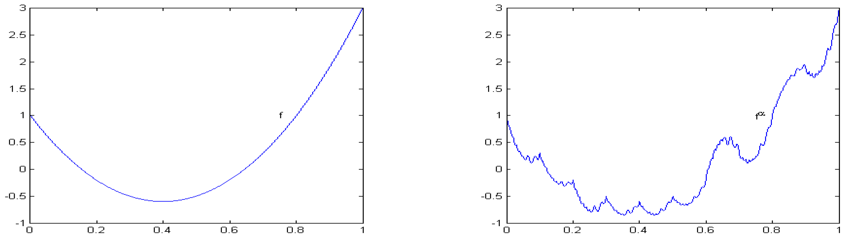
Figure 1 displays the graph of the $\alpha$-fractal function $f^{\alpha }$ corresponding to the function $f\left(x\right)=10x^2-8x+1$ with the base function $b\left(x\right)=2x+1$ on $[0,1]$ for the scale vector $\alpha =(0.15,0.1,0.15,0.1,0.1,0.1,-0.2,0.15,-0.1,0.2)$ and the partition $\Delta :0<0.1<0.2<0.3<0.4<0.5<0.6<0.7<0.8<0.9<1$ of the interval $[0,1]$. We consider $r=1$.

Throughout the article, let $\xi ={\left[{\displaystyle \frac{{\rho }_1}{{\rho }_0}}{\sum }_{i=1}^N{\displaystyle \frac{{\left|{\alpha }_i\right|}^2}{a_i^{2r-1}}}\right]}^{{\displaystyle \frac{1}{2}}}$. The exponent $2r-1$ is obviously related to the degree of regularity of the mappings considered. High orders of smoothness make the construction of fractal functions in weighted Sobolev spaces difficult, according to condition (10). The same is true for large variations of the weight $\rho .$

Regarding the contractive character of the operator T (and consequently the existence of $\alpha$-fractal functions in weighted Sobolev spaces), the case $r=1$ is the least restrictive option (considering a fixed weight $\rho$) since $a_i<1$ and consequently $a_i^{-1}<a_i^{-q}$ for $q>1.$ In the case of uniform partitions, $a_i=1/N$, and condition (10) becomes

$$\sum _{i=1}^N{\left|{\alpha }_i\right|}^2<N^{-1}{\rho }_0/{\rho }_1,$$

for the limit case $r=1.$

Proposition 1.

Let $f\in {\mathcal{W}}_{\rho }^{r,2}\left(I\right)$. If the base function b and the scale vector α satisfy the conditions described in Theorem 1, then

$${∥f^{\alpha }-f∥}_{{\mathcal{W}}_{\rho }^{r,2}\left(I\right)}\le \xi {∥f^{\alpha }-b∥}_{{\mathcal{W}}_{\rho }^{r,2}\left(I\right)}$$

and

$${∥f^{\alpha }-f∥}_{{\mathcal{W}}_{\rho }^{r,2}\left(I\right)}\le {\displaystyle \frac{\xi }{1-\xi }}{∥f-b∥}_{{\mathcal{W}}_{\rho }^{r,2}\left(I\right)}.$$

Proof. 

For any $f\in {\mathcal{W}}_{\rho }^{r,2}\left(I\right)$,

$$(f^{\alpha }-f)\left(x\right)={\alpha }_i(f^{\alpha }-b)\left(L_i^{-1}\left(x\right)\right);x\in I_i,i\in J.$$

(19)

Then

$${∥f^{\alpha }-f∥}_{{\mathcal{W}}_{\rho }^{r,2}\left(I\right)}={\left[\begin{array}{c}\sum _{j=0}^{r-1}{\left|{(f^{\alpha }-f)}^{\left(j\right)}\left(x_0\right)\right|}^2\\ +{\int }_I{\left|{(f^{\alpha }-f)}^{\left(r\right)}\left(x\right)\right|}^2\rho \left(x\right)dx\end{array}\right]}^{{\displaystyle \frac{1}{2}}}.$$

(20)

For $j=0,1,2,\dots ,r$ and $x\in I_i,$$i\in J$, we have, from (19),

$${(f^{\alpha }-f)}^{\left(j\right)}\left(x\right)={\displaystyle \frac{{\alpha }_i}{a_i^j}}{(f^{\alpha }-b)}^{\left(j\right)}\left(L_i^{-1}\left(x\right)\right)$$

(21)

Since $0<a_1<1$, then ${\displaystyle \frac{1}{a_1^{2j}}}\le {\displaystyle \frac{1}{a_1^{2(r-1)}}}$ for all $j=0,1,2,\dots ,(r-1)$ and consequently, using (21), we have

$$\begin{array}{ccc}\hfill \sum _{j=0}^{r-1}{\left|{(f^{\alpha }-f)}^{\left(j\right)}\left(x_0\right)\right|}^2& =& \sum _{j=0}^{r-1}{\displaystyle \frac{{\left|{\alpha }_1\right|}^2}{a_1^{2j}}}{\left|{(f^{\alpha }-b)}^{\left(j\right)}\left(L_1^{-1}\left(x_0\right)\right)\right|}^2\hfill \\ & =& \sum _{j=0}^{r-1}{\displaystyle \frac{{\left|{\alpha }_1\right|}^2}{a_1^{2j}}}{\left|{(f^{\alpha }-b)}^{\left(j\right)}\left(x_0\right)\right|}^2\hfill \\ & \le & {\displaystyle \frac{{\left|{\alpha }_1\right|}^2}{a_1^{2r-2}}}\sum _{j=0}^{r-1}{\left|{(f^{\alpha }-b)}^{\left(j\right)}\left(x_0\right)\right|}^2.\hfill \end{array}$$

(22)

Again, using (21),

$$\begin{array}{ccc}\hfill {\int }_I{\left|{(f^{\alpha }-f)}^{\left(r\right)}\left(x\right)\right|}^{2}dx& =& \sum _{i=1}^N{\int }_{I_i}{\left|{(f^{\alpha }-f)}^{\left(r\right)}\left(x\right)\right|}^{2}dx\hfill \\ & =& \sum _{i=1}^N{\int }_{I_i}{\left|{\displaystyle \frac{{\alpha }_i}{a_i^r}}{(f^{\alpha }-b)}^{\left(r\right)}\left(L_i^{-1}\left(x\right)\right)\right|}^{2}dx\hfill \\ & =& \sum _{i=1}^N{\displaystyle \frac{{\left|{\alpha }_i\right|}^2}{a_i^{2r}}}\hfill \\ & & \times {\int }_{I_i}{\left|{(f^{\alpha }-b)}^{\left(r\right)}\left(L_i^{-1}\left(x\right)\right)\right|}^{2}dx.\hfill \end{array}$$

(23)

Substituting $L_i^{-1}\left(x\right)=z$ in (23), we have

$${\int }_I{\left|{(f^{\alpha }-f)}^{\left(r\right)}\left(x\right)\right|}^{2}dx=\left[\sum _{i=1}^N{\displaystyle \frac{{\left|{\alpha }_i\right|}^2}{a_i^{2r-1}}}\right]{\int }_I{\left|{(f^{\alpha }-b)}^{\left(r\right)}\left(z\right)\right|}^{2}dz.$$

(24)

Therefore, using (24),

$$\begin{array}{ccc}\hfill {\int }_I{\left|{(f^{\alpha }-f)}^{\left(r\right)}\left(x\right)\right|}^2\rho \left(x\right)dx& \le & {\rho }_1{\int }_I{\left|{(f^{\alpha }-f)}^{\left(r\right)}\left(x\right)\right|}^{2}dx\hfill \\ & =& {\rho }_1\left[\sum _{i=1}^N{\displaystyle \frac{{\left|{\alpha }_i\right|}^2}{a_i^{2r-1}}}\right]\hfill \\ & & \times {\int }_I{\left|{(f^{\alpha }-b)}^{\left(r\right)}\left(x\right)\right|}^{2}dx\hfill \\ & =& {\displaystyle \frac{{\rho }_1}{{\rho }_0}}\left[\sum _{i=1}^N{\displaystyle \frac{{\left|{\alpha }_i\right|}^2}{a_i^{2r-1}}}\right]\hfill \\ & & \times {\int }_I{\left|{(f^{\alpha }-b)}^{\left(r\right)}\left(x\right)\right|}^2{\rho }_{0}dx\hfill \\ & \le & \left[{\displaystyle \frac{{\rho }_1}{{\rho }_0}}\sum _{i=1}^N{\displaystyle \frac{{\left|{\alpha }_i\right|}^2}{a_i^{2r-1}}}\right]\hfill \\ & & \times {\int }_I{\left|{(f^{\alpha }-b)}^{\left(r\right)}\left(x\right)\right|}^2\rho \left(x\right)dx.\hfill \end{array}$$

(25)

By (22) and (25), we have from (20), the following inequality:

$$\begin{array}{ccc}\hfill {∥f^{\alpha }-f∥}_{{\mathcal{W}}_{\rho }^{r,2}\left(I\right)}^2& =& \sum _{j=0}^{r-1}{\left|{(f^{\alpha }-f)}^{\left(j\right)}\left(x_0\right)\right|}^2\hfill \\ & & +{\int }_I{\left|{(f^{\alpha }-f)}^{\left(r\right)}\left(x\right)\right|}^2\rho \left(x\right)dx\hfill \\ & \le & \left[{\displaystyle \frac{{\left|{\alpha }_1\right|}^2}{a_1^{2r-2}}}\right]\sum _{j=0}^{r-1}{\left|{(f^{\alpha }-b)}^{\left(j\right)}\left(x_0\right)\right|}^2\hfill \\ & & +\left[{\displaystyle \frac{{\rho }_1}{{\rho }_0}}\sum _{i=1}^N{\displaystyle \frac{{\left|{\alpha }_i\right|}^2}{a_i^{2r-1}}}\right]{\int }_I{\left|{(f^{\alpha }-b)}^{\left(r\right)}\left(x\right)\right|}^2\rho \left(x\right)dx\hfill \\ & \le & max\{\left[{\displaystyle \frac{{\left|{\alpha }_1\right|}^2}{a_1^{2r-2}}}\right],\left[{\displaystyle \frac{{\rho }_1}{{\rho }_0}}\sum _{i=1}^N{\displaystyle \frac{{\left|{\alpha }_i\right|}^2}{a_i^{2r-1}}}\right]\}\hfill \\ & & \times \left[\begin{array}{c}\sum _{j=0}^{r-1}{\left|{(f^{\alpha }-b)}^{\left(j\right)}\left(x_0\right)\right|}^2\\ +{\int }_I{\left|{(f^{\alpha }-b)}^{\left(r\right)}\left(x\right)\right|}^2\rho \left(x\right)dx\end{array}\right]\hfill \\ & =& \left[{\displaystyle \frac{{\rho }_1}{{\rho }_0}}\sum _{i=1}^N{\displaystyle \frac{{\left|{\alpha }_i\right|}^2}{a_i^{2r-1}}}\right]{∥f^{\alpha }-b∥}_{{\mathcal{W}}_{\rho }^{r,2}\left(I\right)}^2.\hfill \end{array}$$

Therefore

$${∥f^{\alpha }-f∥}_{{\mathcal{W}}_{\rho }^{r,2}\left(I\right)}\le \xi {∥f^{\alpha }-b∥}_{{\mathcal{W}}_{\rho }^{r,2}\left(I\right)}.$$

The second one can be obtained from the last inequality by using the triangle inequality of the norm. □

Taking $b=Lf$ in Proposition 1, where L is a linear bounded operator satisfying the condition (8) on ${\mathcal{W}}_{\rho }^{r,2}\left(I\right)$, we get the following.

Proposition 2.

Let $f\in {\mathcal{W}}_{\rho }^{r,2}\left(I\right)$. If the base function b and the scale vector α satisfy the conditions described in Theorem 1, and L is linear and bounded with respect to the norm in ${\mathcal{W}}_{\rho }^{r,2}\left(I\right)$, then

$${∥f^{\alpha }-f∥}_{{\mathcal{W}}_{\rho }^{r,2}\left(I\right)}\le {\displaystyle \frac{\xi }{1-\xi }}{∥Id-L∥}_{{\mathcal{W}}_{\rho }^{r,2}\left(I\right)}{∥f∥}_{{\mathcal{W}}_{\rho }^{r,2}\left(I\right)},$$

where $Id$ is the identity operator on ${\mathcal{W}}_{\rho }^{r,2}\left(I\right)$.

Proposition 3.

With scale vector α satisfying conditions (9) and (10), and L fulfilling the hypotheses of the previous proposition, the operator ${\mathcal{F}}^{\alpha }:{\mathcal{W}}_{\rho }^{r,2}\left(I\right)\to {\mathcal{W}}_{\rho }^{r,2}\left(I\right)$ defined by

$${\mathcal{F}}^{\alpha }\left(f\right)=f^{\alpha },\mathit{\text{for}}\mathit{\text{all}}f\in {\mathcal{W}}_{\rho }^{r,2}\left(I\right),$$

is linear and bounded.

Proof. 

The linearity of ${\mathcal{F}}^{\alpha }$ is obvious. Using Proposition 2, we have

$$\begin{array}{ccc}\hfill {∥{\mathcal{F}}^{\alpha }\left(f\right)∥}_{{\mathcal{W}}_{\rho }^{r,2}\left(I\right)}& =& {∥f^{\alpha }∥}_{{\mathcal{W}}_{\rho }^{r,2}\left(I\right)}\hfill \\ & \le & {∥f^{\alpha }-f∥}_{{\mathcal{W}}_{\rho }^{r,2}\left(I\right)}+{∥f∥}_{{\mathcal{W}}_{\rho }^{r,2}\left(I\right)}\hfill \\ & \le & {\displaystyle \frac{\xi }{1-\xi }}{∥Id-L∥}_{{\mathcal{W}}_{\rho }^{r,2}\left(I\right)}{∥f∥}_{{\mathcal{W}}_{\rho }^{r,2}\left(I\right)}+{∥f∥}_{{\mathcal{W}}_{\rho }^{r,2}\left(I\right)}\hfill \\ & =& \left(1+{\displaystyle \frac{\xi }{1-\xi }}{∥Id-L∥}_{{\mathcal{W}}_{\rho }^{r,2}\left(I\right)}\right){∥f∥}_{{\mathcal{W}}_{\rho }^{r,2}\left(I\right)}.\hfill \end{array}$$

The boundedness follows from the above inequality. □

4. Convergence of Sequences of Fractal Functions

In this section, we discuss the uniform convergence and the convergence with respect to the weighted Sobolev norm of the sequences of the $\alpha$-fractal functions corresponding to the Sobolev functions.

Theorem 2.

Let ${\left\{f_n\right\}}_{n=1}^{\infty }$ and ${\left\{b_n\right\}}_{n=1}^{\infty }$ be the sequences of functions in ${\mathcal{W}}_{\rho }^{r,2}\left(I\right)$ converging uniformly to f and b respectively. Suppose that for every $n\in \mathbb{N}$, $f_n^{\alpha }$ is the α-fractal function of $f_n$ with the base function $b_n$ and $f^{\alpha }$ is the α-fractal function of f with base function b. Then, ${\left\{f_n^{\alpha }\right\}}_{n=1}^{\infty }$ converges uniformly to $f^{\alpha }$ on I.

Proof. 

For $x\in I_i,i\in J$, we have

$$f^{\alpha }\left(x\right)=f\left(x\right)+{\alpha }_i(f^{\alpha }-b)\left(L_i^{-1}\left(x\right)\right)$$

and

$$f_n^{\alpha }\left(x\right)=f_n\left(x\right)+{\alpha }_i(f_n^{\alpha }-b_n)\left(L_i^{-1}\left(x\right)\right).$$

Therefore

$$\begin{array}{ccc}\hfill f_n^{\alpha }\left(x\right)-f^{\alpha }\left(x\right)& =& f_n\left(x\right)-f\left(x\right)+{\alpha }_i(f_n^{\alpha }-f^{\alpha })\left(L_i^{-1}\left(x\right)\right)\hfill \\ & & -{\alpha }_i(b_n-b)\left(L_i^{-1}\left(x\right)\right).\hfill \end{array}$$

Then

$$\begin{array}{ccc}\hfill \underset{x\in I_i}{sup}\left|f_n^{\alpha }\left(x\right)-f^{\alpha }\left(x\right)\right|& \le & {∥f_n-f∥}_{\infty }+{\left|\alpha \right|}_{\infty }{∥f_n^{\alpha }-f^{\alpha }∥}_{\infty }\hfill \\ & & +{\left|\alpha \right|}_{\infty }{∥b_n-b∥}_{\infty }.\hfill \end{array}$$

It follows that

$${∥f_n^{\alpha }-f^{\alpha }∥}_{\infty }\le {∥f_n-f∥}_{\infty }+{\left|\alpha \right|}_{\infty }{∥f_n^{\alpha }-f^{\alpha }∥}_{\infty }+{\left|\alpha \right|}_{\infty }{∥b_n-b∥}_{\infty },$$

so that

$${∥f_n^{\alpha }-f^{\alpha }∥}_{\infty }\le {\displaystyle \frac{1}{1-{\left|\alpha \right|}_{\infty }}}{∥f_n-f∥}_{\infty }+{\displaystyle \frac{{\left|\alpha \right|}_{\infty }}{1-{\left|\alpha \right|}_{\infty }}}{∥b_n-b∥}_{\infty }.$$

Since ${\left|\alpha \right|}_{\infty }<1$, then the uniform convergence of ${\left\{f_n\right\}}_{n=1}^{\infty }$ and ${\left\{b_n\right\}}_{n=1}^{\infty }$ gives the desired result. □

We can prove the following results directly from the linearity of the operator ${\mathcal{F}}^{\alpha }$ defined in Proposition 3.

Lemma 1.

Let $f,g,b$ and c be functions in ${\mathcal{W}}_{\rho }^{r,2}\left(I\right)$. Suppose that $f^{\alpha },g^{\alpha }$ are the α-fractal functions of $f,g$ with the base functions $b,c$ respectively. Let $p,q\in \mathbb{R}$, then $p{f}^{\alpha }+q{g}^{\alpha }$ is also the α-fractal function of $pf+qg$ with base function $pb+qc$. That is,

$${(pf+qg)}^{\alpha }=p{f}^{\alpha }+q{g}^{\alpha }.$$

Theorem 3.

Let ${\left\{f_n\right\}}_{n=1}^{\infty }$ and ${\left\{b_n\right\}}_{n=1}^{\infty }$ be sequences of functions in ${\mathcal{W}}_{\rho }^{r,2}\left(I\right)$ converging to f and b respectively in ${\mathcal{W}}_{\rho }^{r,2}\left(I\right)$ with respect to the weighted Sobolev norm. Suppose that for every $n\in \mathbb{N}$, $f_n^{\alpha }$ is the corresponding α-fractal function of $f_n$ with the base function $b_n$ and let $f^{\alpha }$ be the α-fractal function of f with base function b. Then, ${\left\{f_n^{\alpha }\right\}}_{n=1}^{\infty }$ converges in the weighted Sobolev norm to $f^{\alpha }$ on I.

Proof. 

From Proposition 1 and Lemma 1,

$$\begin{array}{ccc}\hfill {∥(f_n^{\alpha }-f^{\alpha })-(f_n-f)∥}_{{\mathcal{W}}_{\rho }^{r,2}\left(I\right)}& \le & {\displaystyle \frac{\xi }{1-\xi }}\hfill \\ & & \times \left[{∥(f_n-f)-(b_n-b)∥}_{{\mathcal{W}}_{\rho }^{r,2}\left(I\right)}\right]\hfill \\ & \le & {\displaystyle \frac{\xi }{1-\xi }}{∥f_n-f∥}_{{\mathcal{W}}_{\rho }^{r,2}\left(I\right)}\hfill \\ & & +{\displaystyle \frac{\xi }{1-\xi }}{∥b_n-b∥}_{{\mathcal{W}}_{\rho }^{r,2}\left(I\right)}.\hfill \end{array}$$

Therefore

$$\begin{array}{ccc}\hfill {∥f_n^{\alpha }-f^{\alpha }∥}_{{\mathcal{W}}_{\rho }^{r,2}\left(I\right)}& \le & {∥(f_n^{\alpha }-f^{\alpha })-(f_n-f)∥}_{{\mathcal{W}}_{\rho }^{r,2}\left(I\right)}\hfill \\ & & +{∥f_n-f∥}_{{\mathcal{W}}_{\rho }^{r,2}\left(I\right)}\hfill \\ & \le & {\displaystyle \frac{\xi }{1-\xi }}{∥f_n-f∥}_{{\mathcal{W}}_{\rho }^{r,2}\left(I\right)}+{\displaystyle \frac{\xi }{1-\xi }}{∥b_n-b∥}_{{\mathcal{W}}_{\rho }^{r,2}\left(I\right)}\hfill \\ & & +{∥f_n-f∥}_{{\mathcal{W}}_{\rho }^{r,2}\left(I\right)}\hfill \\ & =& {\displaystyle \frac{1}{1-\xi }}{∥f_n-f∥}_{{\mathcal{W}}_{\rho }^{r,2}\left(I\right)}\hfill \\ & & +{\displaystyle \frac{\xi }{1-\xi }}{∥b_n-b∥}_{{\mathcal{W}}_{\rho }^{r,2}\left(I\right)}.\hfill \end{array}$$

Since $\xi <1$, the desired result follows from convergence in weighted Sobolev norm of ${\left\{f_n\right\}}_{n=1}^{\infty }$ and ${\left\{b_n\right\}}_{n=1}^{\infty }$. □

5. Fractional Calculus on Fractal Functions

We show in this section that the Riemann–Liouville fractional order integral $I_{x_0}^{\nu }{f}^{\alpha }$ of $f^{\alpha }$ corresponding to any $f\in {\mathcal{W}}_{\rho }^{r,2}\left(I\right)$ is a FIF, associated with a contractive operator, that satisfies a self-referential equation and interpolates a set of new data points. The function $I_{x_0}^{\nu }{f}^{\alpha }$ is an $\alpha$-fractal function of $I_{x_0}^{\nu }f$ with the base function $I_{x_0}^{\nu }b$, if the functions $I_{x_0}^{\nu }f$ and $I_{x_0}^{\nu }b$ and the scale factors satisfy the conditions described in Theorem 1. Also, we provide a discussion about the convergence of sequences of fractional order integral of $\alpha$-fractal functions.

The Riemann–Liouville fractional integral operator is related to weak derivatives on weighted spaces, specially in the context of Sobolev and Morrey spaces. Some results about this interaction can be found in references [21,22,23].

To prove the main results in this section, we need first to establish some lemmas.

Lemma 2.

The following statements hold:

$\left(i\right)$ If $f\in \mathcal{C}\left(I\right)$ and $\nu \in {\mathbb{R}}^{+}$ the set of positive reals, then $I_{x_0}^{\nu }f\in {\mathcal{C}}^{\left[\nu \right]}\left(I\right)$.

$\left(ii\right)$ If $f\in {\mathcal{C}}^r\left(I\right)$, $r\in \mathbb{N}$ and $\nu \in \mathbb{N}$, then $I_{x_0}^{\nu }f\in {\mathcal{C}}^{\nu +r}\left(I\right)\subset {\mathcal{C}}^r\left(I\right)$.

$\left(iii\right)$ If $f\in {\mathcal{C}}^r\left(I\right)$, $r\in \mathbb{N}$ and $\nu \in {\mathbb{R}}^{+}$ with $\nu \ge r$ or $\nu \in \mathbb{N}$ with $\nu <r$, then $I_{x_0}^{\nu }f\in {\mathcal{C}}^r\left(I\right)$.

$\left(iv\right)$ If $f\in {\mathcal{W}}_{\rho }^{r,2}\left(I\right)$, $r\in \mathbb{N}$ and $\nu \in {\mathbb{R}}^{+}$ with $\nu \ge r$ or $\nu \in \mathbb{N}$ with $\nu <r$, then $I_{x_0}^{\nu }f\in {\mathcal{W}}_{\rho }^{r,2}\left(I\right)$.

Here $\left[\nu \right]$ means the largest integer less than or equal to ν.

Proof. 

These are standard results of fractional integral calculus. □

Lemma 3.

Let ${\left\{f_n\right\}}_{n=1}^{\infty }$ be any sequence in ${\mathcal{W}}_{\rho }^{r,2}\left(I\right)$ converging uniformly to f. Suppose that $\nu \in {\mathbb{R}}^{+}$ with $\nu \ge r$ or $\nu \in \mathbb{N}$ with $\nu <r$. Then ${\left\{I_{x_0}^{\nu }{f}_n\right\}}_{n=1}^{\infty }$ converges uniformly to $I_{x_0}^{\nu }f$.

Proof. 

Since each $f_n\in {\mathcal{W}}_{\rho }^{r,2}\left(I\right)$, then by Lemma 2, $I_{x_0}^{\nu }{f}_n\in {\mathcal{W}}_{\rho }^{r,2}\left(I\right)$.

Let $\epsilon >0$ be given; then there is $N\in \mathbb{N}$ such that for $n\ge N$ and for all $t\in I$,

$$\left|f_n\left(t\right)-f\left(t\right)\right|<{\displaystyle \frac{\epsilon \mathsf{\Gamma }\left(\nu \right)}{{(x_N-x_0)}^{\nu }}}.$$

(26)

Using (26), for all $x\in I$ and for $n\ge N$,

$$\begin{array}{ccc}\hfill \left|I_{x_0}^{\nu }{f}_n\left(x\right)-I_{x_0}^{\nu }f\left(x\right)\right|& =& {\displaystyle \frac{1}{\mathsf{\Gamma }\left(\nu \right)}}\left|\begin{array}{c}{\int }_{x_0}^x{(x-t)}^{\nu -1}{f}_n\left(t\right)dt\\ -{\int }_{x_0}^x{(x-t)}^{\nu -1}f\left(t\right)dt\end{array}\right|\hfill \\ & \le & {\displaystyle \frac{1}{\mathsf{\Gamma }\left(\nu \right)}}{\int }_{x_0}^x{\left|x-t\right|}^{\nu -1}\left|f_n\left(t\right)-f\left(t\right)\right|dt\hfill \\ & \le & {\displaystyle \frac{\epsilon }{{(x_N-x_0)}^{\nu }}}{(x_N-x_0)}^{\nu -1}{\int }_{x_0}^{x}dt\hfill \\ & =& {\displaystyle \frac{\epsilon }{(x_N-x_0)}}{\int }_{x_0}^{x}dt\hfill \\ & <& \epsilon .\hfill \end{array}$$

This shows that ${\left\{I_{x_0}^{\nu }{f}_n\right\}}_{n=1}^{\infty }$ converges uniformly to $I_{x_0}^{\nu }{f}^{\alpha }$ on I. □

Lemma 4.

Let ${\left\{f_n\right\}}_{n=1}^{\infty }$ be any sequence in ${\mathcal{W}}_{\rho }^{r,2}\left(I\right)$ converging in ${\mathcal{L}}_{\rho }^2\left(I\right)$-norm to f. Suppose that ν is any real such that $\nu \ge r+1$. Then, the sequence ${\left\{{\left(I_{x_0}^{\nu }{f}_n\right)}^{\left(r\right)}\right\}}_{n=1}^{\infty }$ converges in ${\mathcal{L}}_{\rho }^2\left(I\right)$-norm to ${\left(I_{x_0}^{\nu }f\right)}^{\left(r\right)}$.

Proof. 

Given

$${∥f_n-f∥}_{{\mathcal{L}}_{\rho }^2\left(I\right)}\to 0\mathrm{as}n\to \infty .$$

(27)

Suppose that $\nu \in {\mathbb{R}}^{+}\setminus \mathbb{N}$. For $j=0,1,2,\dots ,\left[\nu \right]$ and for any $g\in {\mathcal{W}}_{\rho }^{r,2}\left(I\right)$,

$${\left(I_{x_0}^{\nu }g\right)}^{\left(j\right)}\left(x\right)={\displaystyle \frac{1}{\mathsf{\Gamma }(\nu -j)}}{\int }_{x_0}^x{(x-t)}^{(\nu -1)-j}g\left(t\right)dt.$$

Therefore, using Hölder’s inequality, for all $x\in I$,

$$\begin{array}{ccc}& & \left|{\left(I_{x_0}^{\nu }{f}_n\right)}^{\left(r\right)}\left(x\right)-{\left(I_{x_0}^{\nu }f\right)}^{\left(r\right)}\left(x\right)\right|\hfill \\ & =& \left|\begin{array}{c}{\displaystyle \frac{1}{\mathsf{\Gamma }(\nu -r)}}{\int }_{x_0}^x{(x-t)}^{(\nu -1)-r}{f}_n\left(t\right)dt\\ -{\displaystyle \frac{1}{\mathsf{\Gamma }(\nu -r)}}{\int }_{x_0}^x{(x-t)}^{(\nu -1)-r}f\left(t\right)dt\end{array}\right|\hfill \\ & =& {\displaystyle \frac{1}{\mathsf{\Gamma }(\nu -r)}}\left|{\int }_{x_0}^x{(x-t)}^{(\nu -1)-r}(f_n-f)\left(t\right)dt\right|\hfill \\ & \le & {\displaystyle \frac{1}{\mathsf{\Gamma }(\nu -r)}}{\int }_{x_0}^x{\left|x-t\right|}^{(\nu -1)-r}\left|f_n\left(t\right)-f\left(t\right)\right|dt\hfill \\ & \le & {\displaystyle \frac{{(x_N-x_0)}^{(\nu -1)-r}}{\mathsf{\Gamma }(\nu -r)}}{\int }_{x_0}^x\left|f_n\left(t\right)-f\left(t\right)\right|dt\hfill \\ & \le & {\displaystyle \frac{{(x_N-x_0)}^{(\nu -1)-r}}{\mathsf{\Gamma }(\nu -r)}}{\left({\int }_{x_0}^x{\displaystyle \frac{1}{\rho \left(t\right)}}dt\right)}^{{\displaystyle \frac{1}{2}}}\hfill \\ & & \times {\left({\int }_{x_0}^x{\left|f_n\left(t\right)-f\left(t\right)\right|}^2\rho \left(t\right)dt\right)}^{{\displaystyle \frac{1}{2}}}\hfill \\ & \le & {\displaystyle \frac{{(x_N-x_0)}^{(\nu -1)-r}}{\mathsf{\Gamma }(\nu -r)}}{\left({\int }_{x_0}^{x_N}{\displaystyle \frac{1}{\rho \left(t\right)}}dt\right)}^{{\displaystyle \frac{1}{2}}}\hfill \\ & & \times {\left({\int }_{x_0}^{x_N}{\left|f_n\left(t\right)-f\left(t\right)\right|}^2\rho \left(t\right)dt\right)}^{{\displaystyle \frac{1}{2}}}\hfill \\ & =& {\displaystyle \frac{{(x_N-x_0)}^{(\nu -1)-r}}{\mathsf{\Gamma }(\nu -r)}}{\left({\int }_{x_0}^{x_N}{\displaystyle \frac{1}{\rho \left(t\right)}}dt\right)}^{{\displaystyle \frac{1}{2}}}\hfill \\ & & \times {∥f_n-f∥}_{{\mathcal{L}}_{\rho }^2\left(I\right)}.\hfill \end{array}$$

(28)

In view of (27) and (28),

$$\begin{array}{ccc}\hfill {∥{\left(I_{x_0}^{\nu }{f}_n\right)}^{\left(r\right)}-{\left(I_{x_0}^{\nu }f\right)}^{\left(r\right)}∥}_{{\mathcal{L}}_{\rho }^2\left(I\right)}^2& =& {\int }_I{\left|{(I_{x_0}^{\nu }{f}_n-I_{x_0}^{\nu }f)}^{\left(r\right)}\left(x\right)\right|}^2\rho \left(x\right)dx\hfill \\ & \to & 0\mathrm{as}n\to \infty .\hfill \end{array}$$

Again, let $\nu \in \mathbb{N}.$ Then, for $j=0,1,\dots ,(\nu -1)$ and for any $g\in {\mathcal{W}}_{\rho }^{r,2}\left(I\right)$,

$${\left(I_{x_0}^{\nu }g\right)}^{\left(j\right)}\left(x\right)={\displaystyle \frac{1}{\mathsf{\Gamma }(\nu -j)}}{\int }_{x_0}^x{(x-t)}^{(\nu -1)-j}g\left(t\right)dt,$$

(29)

Since $\nu -1\ge r$, then (29) is also valid for $j=r$ and therefore, as in the previous case, we can conclude that

$${∥{\left(I_{x_0}^{\nu }{f}_n\right)}^{\left(r\right)}-{\left(I_{x_0}^{\nu }f\right)}^{\left(r\right)}∥}_{{\mathcal{L}}_{\rho }^2\left(I\right)}\to 0\mathrm{as}n\to \infty .$$

□

Lemma 5.

Let ${\left\{f_n\right\}}_{n=1}^{\infty }$ be any sequence in ${\mathcal{W}}_{\rho }^{r,2}\left(I\right)$ converging in ${\mathcal{L}}_{\rho }^2\left(I\right)$ norm to f. Suppose that ν is any real with $\nu \ge r+1$. Then ${\left\{I_{x_0}^{\nu }{f}_n\right\}}_{n=1}^{\infty }$ converges in weighted Sobolev norm to $I_{x_0}^{\nu }f$.

Proof. 

Let $\nu \in {\mathbb{R}}^{+}\setminus \mathbb{N}$. For $j=0,1,2,\dots ,\left[\nu \right]$ and for any $f\in {\mathcal{W}}_{\rho }^{r,2}\left(I\right)$, we have

$${\left(I_{x_0}^{\nu }f\right)}^{\left(j\right)}\left(x\right)={\displaystyle \frac{1}{\mathsf{\Gamma }(\nu -j)}}{\int }_{x_0}^x{(x-t)}^{(\nu -1)-j}f\left(t\right)dt.$$

Therefore, for $j=0,1,2,\dots ,(r-1)$,

$${\left(I_{x_0}^{\nu }{f}_n-I_{x_0}^{\nu }f\right)}^{\left(j\right)}\left(x_0\right)=0.$$

$$\begin{array}{ccc}\hfill {∥I_{x_0}^{\nu }{f}_n-I_{x_0}^{\nu }f∥}_{{\mathcal{W}}_{\rho }^{r,2}\left(I\right)}& =& {\left[\begin{array}{c}\sum _{j=0}^{r-1}{\left|{(I_{x_0}^{\nu }{f}_n-I_{x_0}^{\nu }f)}^{\left(j\right)}\left(x_0\right)\right|}^2\\ +{\int }_I{\left|{(I_{x_0}^{\nu }{f}_n-I_{x_0}^{\nu }f)}^{\left(r\right)}\left(x\right)\right|}^2\rho \left(x\right)dx\end{array}\right]}^{{\displaystyle \frac{1}{2}}}\hfill \\ & =& {\left[{\int }_I{\left|{(I_{x_0}^{\nu }{f}_n-I_{x_0}^{\nu }f)}^{\left(r\right)}\left(x\right)\right|}^2\rho \left(x\right)dx\right]}^{{\displaystyle \frac{1}{2}}}\hfill \\ & =& {∥{(I_{x_0}^{\nu }{f}_n-I_{x_0}^{\nu }f)}^{\left(r\right)}∥}_{{\mathcal{L}}_{\rho }^2\left(I\right)}\to 0\mathrm{as}n\to \infty ,\hfill \end{array}$$

using Lemma 4. Again, we consider the case $\nu \in \mathbb{N}$ with $\nu >r.$ Then, for $j=0,1,\dots (r-1),r,\dots ,(\nu -1)$ and for any $f\in {\mathcal{W}}_{\rho }^{r,2}\left(I\right)$,

$${\left(I_{x_0}^{\nu }f\right)}^{\left(j\right)}\left(x\right)={\displaystyle \frac{1}{\mathsf{\Gamma }(\nu -j)}}{\int }_{x_0}^x{(x-t)}^{(\nu -1)-j}f\left(t\right)dt.$$

Using similar arguments, we can conclude that

$${∥I_{x_0}^{\nu }{f}_n-I_{x_0}^{\nu }f∥}_{{\mathcal{W}}_{\rho }^{r,2}\left(I\right)}\to 0\mathrm{as}n\to \infty .$$

□

The following theorem is one of the main results of this section.

Theorem 4.

Let $f\in {\mathcal{W}}_{\rho }^{r,2}\left(I\right)$ and $\nu \in {\mathbb{R}}^{+}$ with $\nu \ge r$. Let $f^{\alpha }$ be the α-fractal function of f with base function b in ${\mathcal{W}}_{\rho }^{r,2}\left(I\right).$ Suppose that $I_{x_0}^{\nu }f$, $I_{x_0}^{\nu }b$ and the scale factors satisfy the conditions described in Theorem 1. Then $I_{x_0}^{\nu }{f}^{\alpha }$ is the FIF for the RB operator $T^{\nu }:{\mathcal{W}}_{\rho }^{r,2}\left(I\right)\to {\mathcal{W}}_{\rho }^{r,2}\left(I\right)$ defined by

$$T^{\nu }g\left(L_i\left(x\right)\right)=I_{x_0}^{\nu }f\left(L_i\left(x\right)\right)+{\alpha }_i(g-I_{x_0}^{\nu }b)\left(x\right);x\in I,i\in J,$$

(30)

and $I_{x_0}^{\nu }{f}^{\alpha }$ interpolates the points ${\left\{(x_i,y_i^{\nu })\right\}}_{i=0}^N$, where

$$\begin{array}{ccc}\hfill y_0^{\nu }& =& 0,\hfill \\ \hfill y_i^{\nu }& =& I_{x_0}^{\nu }f\left(x_i\right);i=1,2,\dots ,(N-1).\hfill \\ \hfill y_N^{\nu }& =& {\displaystyle \frac{1}{1-{\alpha }_N}}{I}_{x_0}^{\nu }f\left(x_N\right)-{\displaystyle \frac{{\alpha }_N}{1-{\alpha }_N}}{I}_{x_0}^{\nu }b\left(x_N\right).\hfill \end{array}$$

Furthermore, $I_{x_0}^{\nu }{f}^{\alpha }$ satisfies the self-referential equation, for $i\in J$,

$$I_{x_0}^{\nu }{f}^{\alpha }\left(L_i\left(x\right)\right)=I_{x_0}^{\nu }f\left(L_i\left(x\right)\right)+{\alpha }_i(I_{x_0}^{\nu }{f}^{\alpha }-I_{x_0}^{\nu }b)\left(x\right);x\in I.$$

(31)

Proof. 

For any $g,h\in {\mathcal{W}}_{\rho }^{r,2}\left(I\right)$,

$$(T^{\nu }g-T^{\nu }h)\left(L_i\left(x\right)\right)={\alpha }_i(g-h)\left(x\right);x\in I,i\in J.$$

(32)

Rewriting (32),

$$(T^{\nu }g-T^{\nu }h)\left(x\right)={\alpha }_i(g-h)\left(L_i^{-1}\left(x\right)\right);x\in I_i,i\in J.$$

Then, using the same arguments of the proof of Theorem 1, we can easily show that for $\xi ={\left[{\displaystyle \frac{{\rho }_1}{{\rho }_0}}{\sum }_{i=1}^N{\displaystyle \frac{{\left|{\alpha }_i\right|}^2}{a_i^{2r-1}}}\right]}^{{\displaystyle \frac{1}{2}}}<1$, $T^{\nu }$ is a contraction on ${\mathcal{W}}_{\rho }^{r,2}\left(I\right)$. The self-referential equation for $f^{\alpha }$:

$$f^{\alpha }\left(L_i\left(x\right)\right)=f\left(L_i\left(x\right)\right)+{\alpha }_i(f^{\alpha }-b)\left(x\right);x\in I,i\in J.$$

Therefore, for $x\in I,$$i\in J,$

$$\begin{array}{ccc}\hfill I_{x_0}^{\nu }{f}^{\alpha }\left(L_i\left(x\right)\right)& =& {\displaystyle \frac{1}{\mathsf{\Gamma }\left(\nu \right)}}{\int }_{x_0}^x{(x-t)}^{\nu -1}{f}^{\alpha }\left(L_i\left(t\right)\right)dt\hfill \\ & =& {\displaystyle \frac{1}{\mathsf{\Gamma }\left(\nu \right)}}{\int }_{x_0}^x{(x-t)}^{\nu -1}\left[f\left(L_i\left(t\right)\right)+{\alpha }_i(f^{\alpha }-b)\left(t\right)\right]dt\hfill \\ & =& {\displaystyle \frac{1}{\mathsf{\Gamma }\left(\nu \right)}}{\int }_{x_0}^x{(x-t)}^{\nu -1}f\left(L_i\left(t\right)\right)dt\hfill \\ & & +{\alpha }_i{\displaystyle \frac{1}{\mathsf{\Gamma }\left(\nu \right)}}{\int }_{x_0}^x{(x-t)}^{\nu -1}(f^{\alpha }-b)\left(t\right)dt\hfill \\ & =& I_{x_0}^{\nu }f\left(L_i\left(x\right)\right)+{\alpha }_i{I}_{x_0}^{\nu }(f^{\alpha }-b)\left(x\right)\hfill \\ & =& I_{x_0}^{\nu }f\left(L_i\left(x\right)\right)+{\alpha }_i(I_{x_0}^{\nu }{f}^{\alpha }-I_{x_0}^{\nu }b)\left(x\right)\hfill \end{array}$$

(33)

Putting $g=I_{x_0}^{\nu }{f}^{\alpha }$ in (30), we have, for $i\in J$,

$$T^{\nu }{I}_{x_0}^{\nu }{f}^{\alpha }\left(L_i\left(x\right)\right)=I_{x_0}^{\nu }f\left(L_i\left(x\right)\right)+{\alpha }_i(I_{x_0}^{\nu }{f}^{\alpha }-I_{x_0}^{\nu }b)\left(x\right);x\in I.$$

(34)

From (33) and (34), it follows that $T^{\nu }{I}_{x_0}^{\nu }{f}^{\alpha }=I_{x_0}^{\nu }{f}^{\alpha }$. Since $T^{\nu }$ is a contraction, then $I_{x_0}^{\nu }{f}^{\alpha }$ is the unique fixed point of $T^{\nu }$ and consequently, $I_{x_0}^{\nu }{f}^{\alpha }$ is the FIF for the RB operator $T^{\nu }$. This FIF complies with the following self-referential equation

$$I_{x_0}^{\nu }{f}^{\alpha }\left(L_i\left(x\right)\right)=I_{x_0}^{\nu }f\left(L_i\left(x\right)\right)+{\alpha }_i(I_{x_0}^{\nu }{f}^{\alpha }-I_{x_0}^{\nu }b)\left(x\right);x\in I,i\in J.$$

(35)

Now, for $i\in J,$$L_i\left(x_0\right)=x_{i-1}$ and using (35),

$$\begin{array}{ccc}\hfill y_{i-1}^{\nu }& =& I_{x_0}^{\nu }{f}^{\alpha }\left(x_{i-1}\right)\hfill \\ & =& I_{x_0}^{\nu }{f}^{\alpha }\left(L_i\left(x_0\right)\right)\hfill \\ & =& I_{x_0}^{\nu }f\left(L_i\left(x_0\right)\right)+{\alpha }_i(I_{x_0}^{\nu }{f}^{\alpha }-I_{x_0}^{\nu }b)\left(x_0\right)\hfill \\ & =& I_{x_0}^{\nu }f\left(x_{i-1}\right).\hfill \end{array}$$

In particular, $y_0^{\nu }=I_{x_0}^{\nu }f\left(x_0\right)=0$. Again,

$$\begin{array}{ccc}\hfill I_{x_0}^{\nu }{f}^{\alpha }\left(x_N\right)& =& I_{x_0}^{\nu }{f}^{\alpha }\left(L_N\left(x_N\right)\right)\hfill \\ & =& I_{x_0}^{\nu }f\left(L_N\left(x_N\right)\right)+{\alpha }_N(I_{x_0}^{\nu }{f}^{\alpha }-I_{x_0}^{\nu }b)\left(x_N\right)\hfill \\ & =& I_{x_0}^{\nu }f\left(x_N\right)+{\alpha }_N(I_{x_0}^{\nu }{f}^{\alpha }-I_{x_0}^{\nu }b)\left(x_N\right).\hfill \\ & =& I_{x_0}^{\nu }f\left(x_N\right)+{\alpha }_N{I}_{x_0}^{\nu }{f}^{\alpha }\left(x_N\right)-{\alpha }_N{I}_{x_0}^{\nu }b\left(x_N\right).\hfill \end{array}$$

Therefore, from the last line and letting $y_N^{\nu }=I_{x_0}^{\nu }{f}^{\alpha }\left(x_N\right)$, we have

$$\begin{array}{ccc}\hfill y_N^{\nu }& =& {\displaystyle \frac{1}{1-{\alpha }_N}}{I}_{x_0}^{\nu }f\left(x_N\right)-{\displaystyle \frac{{\alpha }_N}{1-{\alpha }_N}}{I}_{x_0}^{\nu }b\left(x_N\right).\hfill \end{array}$$

□

Theorem 4 directly leads to the following corollary.

Corollary 1.

With the hypotheses of the previous theorem, $I_{x_0}^{\nu }{f}^{\alpha }$ is the α-fractal function of $I_{x_0}^{\nu }f$ with base function $I_{x_0}^{\nu }b$ associated with the RB operator (30). That is,

$$\begin{array}{ccc}\hfill {\left(I_{x_0}^{\nu }f\right)}^{\alpha }& =& I_{x_0}^{\nu }{f}^{\alpha }.\hfill \end{array}$$

Example 1.

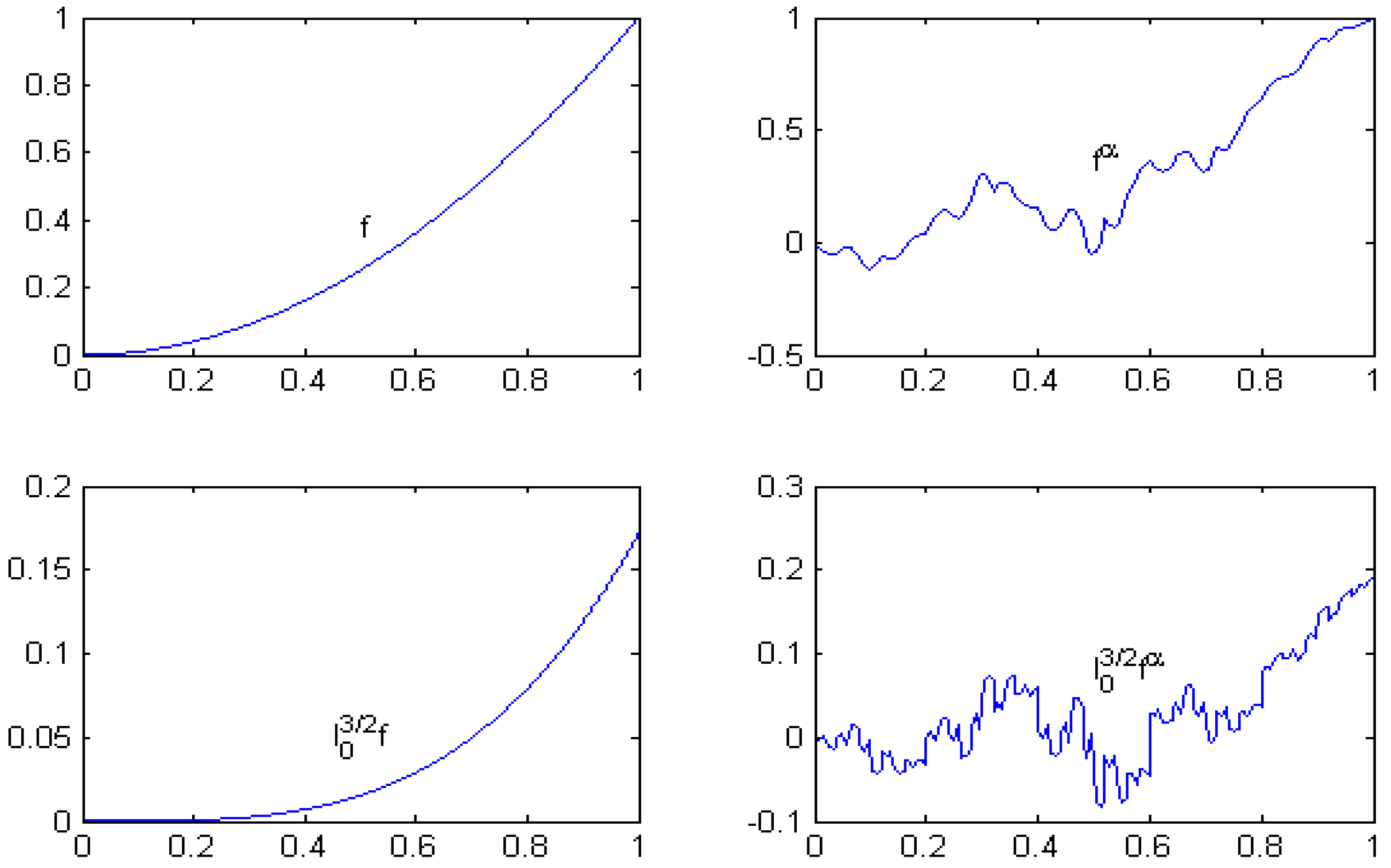
Let $f\left(x\right)=x^2$ defined on $I=[0,1]$ with partition $\Delta :0<0.2<0.4<0.6<0.8<1$. Let us consider the base function $b\left(x\right)=x,$ scale vector $\alpha =(0.3,-0.5,0.7,0.4,-0.2)$ and $r=1.$ The graphical representation of the function f, the corresponding α-fractal function $f^{\alpha }$ and their ${\displaystyle \frac{3}{2}}$-order fractional integrals $I_0^{{\displaystyle \frac{3}{2}}}f$, $I_0^{{\displaystyle \frac{3}{2}}}{f}^{\alpha }$ are shown in Figure 2. The α-fractal function $f^{\alpha }$ presents the typical self-affine oscillations superimposed to the smooth function f. The lower frames of Figure 2 display the action of the operator $I_0^{{\displaystyle \frac{3}{2}}}$ on f and $f^{\alpha }$.

Proposition 4.

Let $f\in {\mathcal{W}}_{\rho }^{r,2}\left(I\right)$ and $\nu \in {\mathbb{R}}^{+}$ with $\nu \ge r$. With the hypotheses of Theorem 4 one has

$${∥I_{x_0}^{\nu }{f}^{\alpha }-I_{x_0}^{\nu }f∥}_{{\mathcal{W}}_{\rho }^{r,2}\left(I\right)}\le \xi {∥I_{x_0}^{\nu }{f}^{\alpha }-I_{x_0}^{\nu }b∥}_{{\mathcal{W}}_{\rho }^{r,2}\left(I\right)}$$

and

$${∥I_{x_0}^{\nu }{f}^{\alpha }-I_{x_0}^{\nu }f∥}_{{\mathcal{W}}_{\rho }^{r,2}\left(I\right)}\le {\displaystyle \frac{\xi }{1-\xi }}{∥I_{x_0}^{\nu }f-I_{x_0}^{\nu }b∥}_{{\mathcal{W}}_{\rho }^{r,2}\left(I\right)},$$

where $\xi ={\displaystyle \frac{{\rho }_1}{{\rho }_0}}\left[{\sum }_{i=1}^N{\displaystyle \frac{{\left|{\alpha }_i\right|}^2}{a_i^{2r-1}}}\right]$.

Proof. 

Theorem 1 and Lemma 2 ensure that $I_{x_0}^{\nu }f,I_{x_0}^{\nu }{f}^{\alpha }\in {\mathcal{W}}_{\rho }^{r,2}\left(I\right)$. Therefore, in similar lines of the proof of Theorem 1, it can be easily shown that

$${∥I_{x_0}^{\nu }{f}^{\alpha }-I_{x_0}^{\nu }f∥}_{{\mathcal{W}}_{\rho }^{r,2}\left(I\right)}\le \xi {∥I_{x_0}^{\nu }{f}^{\alpha }-I_{x_0}^{\nu }b∥}_{{\mathcal{W}}_{\rho }^{r,2}\left(I\right)}.$$

The second inequality is deduced from the triangle inequality of the norm. □

Proposition 5.

Let ${\left\{f_n\right\}}_{n=1}^{\infty }$ and ${\left\{b_n\right\}}_{n=1}^{\infty }$ be sequences of functions in ${\mathcal{W}}_{\rho }^{r,2}\left(I\right)$. Suppose that, for every $n\in \mathbb{N}$, $f_n^{\alpha }$ is the α-fractal function of $f_n$ with base function $b_n$. Also, let $f^{\alpha }$ be the α-fractal function of f with base function b. Let $p,q\in \mathbb{R}$ and $\nu \in {\mathbb{R}}^{+}$ with $\nu \ge r$ or $\nu \in \mathbb{N}$ with $\nu <r$. Then

$$\begin{array}{ccc}& & {∥(p{I}_{x_0}^{\nu }{f}_n^{\alpha }+q{I}_{x_0}^{\nu }{f}^{\alpha })-(p{I}_{x_0}^{\nu }{f}_n+q{I}_{x_0}^{\nu }f)∥}_{{\mathcal{W}}_{\rho }^{r,2}\left(I\right)}\hfill \\ & \le & \xi {∥(p{I}_{x_0}^{\nu }{f}_n^{\alpha }+q{I}_{x_0}^{\nu }{f}^{\alpha })-(p{I}_{x_0}^{\nu }{b}_n+q{I}_{x_0}^{\nu }b)∥}_{{\mathcal{W}}_{\rho }^{r,2}\left(I\right)}\hfill \end{array}$$

and

$$\begin{array}{ccc}& & {∥(p{I}_{x_0}^{\nu }{f}_n^{\alpha }+q{I}_{x_0}^{\nu }{f}^{\alpha })-(p{I}_{x_0}^{\nu }{f}_n+q{I}_{x_0}^{\nu }f)∥}_{{\mathcal{W}}_{\rho }^{r,2}\left(I\right)}\hfill \\ & \le & {\displaystyle \frac{\xi }{1-\xi }}{∥(p{I}_{x_0}^{\nu }{f}_n+q{I}_{x_0}^{\nu }f)-(p{I}_{x_0}^{\nu }{b}_n+q{I}_{x_0}^{\nu }b)∥}_{{\mathcal{W}}_{\rho }^{r,2}\left(I\right)},\hfill \end{array}$$

Proof. 

For $x\in I,$$i\in J$, we have

$$I_{x_0}^{\nu }{f}_n^{\alpha }\left(L_i\left(x\right)\right)=I_{x_0}^{\nu }{f}_n\left(L_i\left(x\right)\right)+{\alpha }_i(I_{x_0}^{\nu }{f}_n^{\alpha }-I_{x_0}^{\nu }{b}_n)\left(x\right)$$

and

$$I_{x_0}^{\nu }{f}^{\alpha }\left(L_i\left(x\right)\right)=I_{x_0}^{\nu }f\left(L_i\left(x\right)\right)+{\alpha }_i(I_{x_0}^{\nu }{f}^{\alpha }-I_{x_0}^{\nu }b)\left(x\right)$$

The following holds

$$\begin{array}{ccc}\hfill (p{I}_{x_0}^{\nu }{f}_n^{\alpha }+q{I}_{x_0}^{\nu }{f}^{\alpha })\left(L_i\left(x\right)\right)& =& (p{I}_{x_0}^{\nu }{f}_n+q{I}_{x_0}^{\nu }f)\left(L_i\left(x\right)\right)\hfill \\ & & +{\alpha }_i\left(\begin{array}{c}(p{I}_{x_0}^{\nu }{f}_n^{\alpha }+q{I}_{x_0}^{\nu }{f}^{\alpha })\\ -(p{I}_{x_0}^{\nu }{b}_n+q{I}_{x_0}^{\nu }b)\end{array}\right)\left(x\right),\hfill \end{array}$$

and we obtain the result. □

The following corollary is an immediate consequence of Proposition 5.

Corollary 2.

Let ${\left\{f_n\right\}}_{n=1}^{\infty }$ and ${\left\{b_n\right\}}_{n=1}^{\infty }$ be two sequences of functions in ${\mathcal{W}}_{\rho }^{r,2}\left(I\right)$. Suppose that, for every $n\in \mathbb{N}$, $f_n^{\alpha }$ is the α-fractal function of $f_n$ with base function $b_n$ and let $f^{\alpha }$ be the α-fractal function of f with base function b. Let $\nu \in {\mathbb{R}}^{+}$ with $\nu \ge r.$ Then

$$\begin{array}{ccc}& & {∥(I_{x_0}^{\nu }{f}_n^{\alpha }-I_{x_0}^{\nu }{f}^{\alpha })-(I_{x_0}^{\nu }{f}_n-I_{x_0}^{\nu }f)∥}_{{\mathcal{W}}_{\rho }^{r,2}\left(I\right)}\hfill \\ & \le & \xi {∥(I_{x_0}^{\nu }{f}_n^{\alpha }-I_{x_0}^{\nu }{f}^{\alpha })-(I_{x_0}^{\nu }{b}_n-I_{x_0}^{\nu }b)∥}_{{\mathcal{W}}_{\rho }^{r,2}\left(I\right)}\hfill \end{array}$$

and

$$\begin{array}{ccc}& & {∥(I_{x_0}^{\nu }{f}_n^{\alpha }-I_{x_0}^{\nu }{f}^{\alpha })-(I_{x_0}^{\nu }{f}_n-I_{x_0}^{\nu }f)∥}_{{\mathcal{W}}_{\rho }^{r,2}\left(I\right)}\hfill \\ & \le & {\displaystyle \frac{\xi }{1-\xi }}{∥(I_{x_0}^{\nu }{f}_n-I_{x_0}^{\nu }f)-(I_{x_0}^{\nu }{b}_n-I_{x_0}^{\nu }b)∥}_{{\mathcal{W}}_{\rho }^{r,2}\left(I\right)},\hfill \end{array}$$

Theorem 5.

Let ${\left\{f_n\right\}}_{n=1}^{\infty }$ and ${\left\{b_n\right\}}_{n=1}^{\infty }$ be sequences of functions in ${\mathcal{W}}_{\rho }^{r,2}\left(I\right)$ converging uniformly to f and b in ${\mathcal{W}}_{\rho }^{r,2}\left(I\right)$ respectively. Suppose that, for every $n\in \mathbb{N}$, $f_n^{\alpha }$ is the α-fractal function of $f_n$ with base function $b_n$ and $f^{\alpha }$ is the α-fractal function of f with base function b. Let $\nu \in {\mathbb{R}}^{+}$ with $\nu \ge r.$ Then, the Riemann–Liouville fractional integrals

$$I_{x_0}^{\nu }{f}_n^{\alpha }\left(x\right)={\displaystyle \frac{1}{\mathsf{\Gamma }\left(\nu \right)}}{\int }_{x_0}^x{(x-t)}^{\nu -1}{f}_n^{\alpha }\left(t\right)dt$$

converge uniformly to

$$I_{x_0}^{\nu }{f}^{\alpha }\left(x\right)={\displaystyle \frac{1}{\mathsf{\Gamma }\left(\nu \right)}}{\int }_{x_0}^x{(x-t)}^{\nu -1}{f}^{\alpha }\left(t\right)dt$$

on I as $n\to \infty$.

Proof. 

Let ${\left\{f_n\right\}}_{n=1}^{\infty }$ be any sequence of functions in ${\mathcal{W}}_{\rho }^{r,2}\left(I\right)$, then the sequence of fractal functions ${\left\{f_n^{\alpha }\right\}}_{n=1}^{\infty }$ is also in ${\mathcal{W}}_{\rho }^{r,2}\left(I\right)$. Since ${\left\{f_n\right\}}_{n=1}^{\infty }$ converges uniformly to $f\in {\mathcal{W}}_{\rho }^{r,2}\left(I\right)$, then by Theorem 2, ${\left\{f_n^{\alpha }\right\}}_{n=1}^{\infty }$ converges uniformly to $f^{\alpha }\in {\mathcal{W}}_{\rho }^{r,2}\left(I\right)$. Applying Lemma 3, we conclude that ${\left\{I_{x_0}^{\nu }{f}_n^{\alpha }\right\}}_{n=1}^{\infty }$ converges uniformly to $I_{x_0}^{\nu }{f}^{\alpha }$. □

For $\nu =1$, Theorem 5 leads to the following corollary.

Corollary 3.

Let ${\left\{f_n\right\}}_{n=1}^{\infty }$ and ${\left\{b_n\right\}}_{n=1}^{\infty }$ be sequences of functions in ${\mathcal{W}}_{\rho }^{1,2}\left(I\right)$ converging uniformly to f and b respectively in ${\mathcal{W}}_{\rho }^{1,2}\left(I\right)$. Suppose that, for every $n\in \mathbb{N}$, $f_n^{\alpha }$ is the α-fractal function of $f_n$ with the base function $b_n$ and $f^{\alpha }$ is the α-fractal function of f with base function b. Then, the integrals ${\int }_{x_0}^x{f}_n^{\alpha }\left(t\right)dt$ converge uniformly to ${\int }_{x_0}^x{f}^{\alpha }\left(t\right)dt$ on I as $n\to \infty$.

Theorem 6.

Let ${\left\{f_n\right\}}_{n=1}^{\infty }$ and ${\left\{b_n\right\}}_{n=1}^{\infty }$ be any sequences of functions in ${\mathcal{W}}_{\rho }^{r,2}\left(I\right)$ converging in ${\mathcal{L}}_{\rho }^2\left(I\right)$-norm to f and b respectively in ${\mathcal{W}}_{\rho }^{r,2}\left(I\right).$ Suppose that, for every $n\in \mathbb{N}$, $f_n^{\alpha }$ is the corresponding α-fractal function of $f_n$ with base function $b_n$ and $f^{\alpha }$ is the α-fractal function of f with base function b. Let ν be any real with $\nu \ge r+1$. Then, the Riemann–Liouville fractional integrals

$$I_{x_0}^{\nu }{f}_n^{\alpha }\left(x\right)={\displaystyle \frac{1}{\mathsf{\Gamma }\left(\nu \right)}}{\int }_{x_0}^x{(x-t)}^{\nu -1}{f}_n^{\alpha }\left(t\right)dt$$

converge in weighted Sobolev norm to

$$I_{x_0}^{\nu }{f}^{\alpha }\left(x\right)={\displaystyle \frac{1}{\mathsf{\Gamma }\left(\nu \right)}}{\int }_{x_0}^x{(x-t)}^{\nu -1}{f}^{\alpha }\left(t\right)dt$$

on I as $n\to \infty$.

Proof. 

From Corollary 2,

$$\begin{array}{ccc}& & {∥(I_{x_0}^{\nu }{f}_n^{\alpha }-I_{x_0}^{\nu }{f}^{\alpha })-(I_{x_0}^{\nu }{f}_n-I_{x_0}^{\nu }f)∥}_{{\mathcal{W}}_{\rho }^{r,2}\left(I\right)}\hfill \\ & \le & {\displaystyle \frac{\xi }{1-\xi }}{∥(I_{x_0}^{\nu }{f}_n-I_{x_0}^{\nu }f)-(I_{x_0}^{\nu }{b}_n-I_{x_0}^{\nu }b)∥}_{{\mathcal{W}}_{\rho }^{r,2}\left(I\right)}\hfill \\ & \le & {\displaystyle \frac{\xi }{1-\xi }}{∥I_{x_0}^{\nu }{f}_n-I_{x_0}^{\nu }f∥}_{{\mathcal{W}}_{\rho }^{r,2}\left(I\right)}+{\displaystyle \frac{\xi }{1-\xi }}{∥I_{x_0}^{\nu }{b}_n-I_{x_0}^{\nu }b∥}_{{\mathcal{W}}_{\rho }^{r,2}\left(I\right)}.\hfill \end{array}$$

Therefore

$$\begin{array}{ccc}& & {∥I_{x_0}^{\nu }{f}_n^{\alpha }-I_{x_0}^{\nu }{f}^{\alpha }∥}_{{\mathcal{W}}_{\rho }^{r,2}\left(I\right)}\hfill \\ & \le & {∥(I_{x_0}^{\nu }{f}_n^{\alpha }-I_{x_0}^{\nu }{f}^{\alpha })-(I_{x_0}^{\nu }{f}_n-I_{x_0}^{\nu }f)∥}_{{\mathcal{W}}_{\rho }^{r,2}\left(I\right)}\hfill \\ & & +{∥I_{x_0}^{\nu }{f}_n-I_{x_0}^{\nu }f∥}_{{\mathcal{W}}_{\rho }^{r,2}\left(I\right)}\hfill \\ & \le & {\displaystyle \frac{\xi }{1-\xi }}{∥I_{x_0}^{\nu }{f}_n-I_{x_0}^{\nu }f∥}_{{\mathcal{W}}_{\rho }^{r,2}\left(I\right)}\hfill \\ & & +{\displaystyle \frac{\xi }{1-\xi }}{∥I_{x_0}^{\nu }{b}_n-I_{x_0}^{\nu }b∥}_{{\mathcal{W}}_{\rho }^{r,2}\left(I\right)}\hfill \\ & & +{∥I_{x_0}^{\nu }{f}_n-I_{x_0}^{\nu }f∥}_{{\mathcal{W}}_{\rho }^{r,2}\left(I\right)}\hfill \\ & =& {\displaystyle \frac{1}{1-\xi }}{∥I_{x_0}^{\nu }{f}_n-I_{x_0}^{\nu }f∥}_{{\mathcal{W}}_{\rho }^{r,2}\left(I\right)}\hfill \\ & & +{\displaystyle \frac{\xi }{1-\xi }}{∥I_{x_0}^{\nu }{b}_n-I_{x_0}^{\nu }b∥}_{{\mathcal{W}}_{\rho }^{r,2}\left(I\right)}.\hfill \end{array}$$

(36)

By Lemma 5,

$${∥I_{x_0}^{\nu }{f}_n-I_{x_0}^{\nu }f∥}_{{\mathcal{W}}_{\rho }^{r,2}\left(I\right)}\to 0\mathrm{as}n\to \infty$$

(37)

and

$${∥I_{x_0}^{\nu }{b}_n-I_{x_0}^{\nu }b∥}_{{\mathcal{W}}_{\rho }^{r,2}\left(I\right)}\to 0\mathrm{as}n\to \infty .$$

(38)

Using (37) and (38), the result follows from (36). □

6. Conclusions

By imposing certain conditions on the base function and the scale vector, we have constructed fractal analogues of any functions from the weighted Sobolev space. It is shown that the fractal version of the uniformly convergent sequence of Sobolev functions remains uniformly convergent and the same fact is verified with respect to the weighted Sobolev norm. Also, it is proved that the Riemann–Liouville fractional order integral of the $\alpha$-fractal function corresponding to any Sobolev function is also a fractal interpolation function that interpolates a specific data points if the base is suitably chosen. Some aspects of the convergence of the Riemann–Liouville integral of $\alpha$-fractal functions when the original mappings converge have been also analyzed.

References

1. Barnsley, M.F. Fractal Everywhere, 2nd ed.; Academic Press: Cambridge, MA, USA, 1993. [Google Scholar]
2. Barnsley, M.F. Fractal functions and interpolation. Constr. Approx. 1986, 2, 303–329. [Google Scholar] [CrossRef]
3. Navascués, M.A. Fractal trigonometric approximation. Electron. Trans. Numer. Anal. 2005, 20, 64–74. [Google Scholar]
4. Akhtar, M.N.; Prasad, M.G.P.; Navascués, M.A. Fractal Jacobi systems and convergence of Fourier-Jacobi expansions of fractal interpolation functions. Mediterr. J. Math. 2016, 13, 3965–3984. [Google Scholar] [CrossRef]
5. Barnsley, M.F.; Harrington, A.N. The calculus of fractal interpolation functions. J. Approx. Theory 1989, 57, 14–34. [Google Scholar] [CrossRef]
6. Navascués, M.A.; Sebastián, M.V. Numerical integration of affine fractal functions. J. Comput. Appl. Math. 2013, 252, 169–176. [Google Scholar] [CrossRef]
7. Pan, X. Fractional calculus of fractal interpolation function on [0,b](b>0). In Abstract and Applied Analysis; Hindawi Publishing Corporation: London, UK, 2014; p. 640628. [Google Scholar] [CrossRef]
8. Agathiyan, A.; Gowrisankar, A.; Priyanka, T.M.C. Construction of new fractal interpolation functions through integration method. Results Math. 2022, 77, 122. [Google Scholar] [CrossRef]
9. Ruan, H.J.; Su, W.Y.; Yao, K. Box dimension and fractional integral of linear fractal interpolation functions. J. Approx. Theory 2009, 161, 187–197. [Google Scholar] [CrossRef]
10. Pan, X.; Xu, R.; Shang, X.; Wang, M. The properties of fractional order calculus of fractal interpolation function of broken line segments. Fractals 2018, 26, 1850031. [Google Scholar] [CrossRef]
11. Priyanka, T.M.C.; Gowrisankar, A. Riemann-Liouville fractional integral of non-affine fractal interpolation function and its fractional operator. Eur. Phys. J. Spec. Top. 2021, 230, 3789–3805. [Google Scholar] [CrossRef]
12. Prasad, S.A. Fractional calculus of coalescence hidden-variable fractal interpolation functions. Fractals 2017, 25, 1750019. [Google Scholar] [CrossRef]
13. Navascués, M.A.; Pacurar, C.; Drakopoulos, V. Scale-free fractal interpolation. Fractal Fract. 2022, 6, 602. [Google Scholar] [CrossRef]
14. García-Sáez, G. Fractional weighted Sobolev spaces associated to the Riesz fractional gradient. arXiv 2025, arXiv:2512.09575. [Google Scholar] [CrossRef]
15. Golmankhaneh, A.K.; Jorgensen, P.E.T.; Serpa, C.; Welch, K. About Sobolev spaces on fractals: Fractal gradients and Laplacians. Aequationes Math. 2025, 99, 465–490. [Google Scholar] [CrossRef]
16. Tan, Q.; Zhou, J.; Wang, Y. Weighted fractional Sobolev spaces on timescales with applications to weighted fractional p-Laplacian systems. Fractal Fract. 2025, 9, 500. [Google Scholar] [CrossRef]
17. Viswanathan, P.; Navascués, M.A. A fractal operator on some standard spaces of functions. Proc. Edinb. Math. Soc. 2017, 60, 771–786. [Google Scholar] [CrossRef]
18. Massopust, P.R. Fractal Functions, Fractal Surfaces, and Wavelets; Academic Press: New York, NY, USA, 1995. [Google Scholar]
19. Sharapudinov, I.I. Sobolev-orthogonal systems of functions associated with an orthogonal system. Izv. Math. 2018, 82, 212–244. [Google Scholar] [CrossRef]
20. Evans, L.C. Partial Differential Equations, Graduate Studies in Mathematics; American Mathematical Society: Providence, RI, USA, 1998; Volume 19. [Google Scholar]
21. Ho, K.-P. Riemann-Liouville and Weyl fractional integral operators on weighted Morrey spaces. Fract. Calc. Appl. Anal. 2025, 28, 3106–3116. [Google Scholar] [CrossRef]
22. Kalybay, A.; Oinarov, R. Boundedness of Riemann-Liouville operator from weighted Sobolev space to weighted Lebesgue space for 1 <q <p <. Math. Ineq. Appl. 2022, 25, 17–26. [Google Scholar] [CrossRef]
23. Othmane, I.B.; Nisse, L.; Abdeljawad, T. On Cauchy-type problems with weighted R-L fractional derivatives of a function with respect to another function and comparison theorems. AIMS Math. 2024, 9, 14106–14129. [Google Scholar] [CrossRef]
Figure 1. The function f ( x ) = 10 x 2 8 x + 1 (left) and its α -fractal function f α ( x ) = ( 10 x 2 8 x + 1 ) α (right). Here α = ( 0.15 , 0.1 , 0.15 , 0.1 , 0.1 , 0.1 , 0.2 , 0.15 , 0.1 , 0.2 ) .
Fractalfract 10 00134 g001
Figure 2. Graphical representation of f ( x ) = x 2 , corresponding α -fractal function f α and their 3 2 -order fractional integrals I 0 3 2 f , I 0 3 2 f α respectively. The scale vector is α = ( 0.3 , 0.5 , 0.7 , 0.4 , 0.2 ) ...
Fractalfract 10 00134 g002
Disclaimer/Publisher’s Note: The statements, opinions and data contained in all publications are solely those of the individual author(s) and contributor(s) and not of MDPI and/or the editor(s). MDPI and/or the editor(s) disclaim responsibility for any injury to people or property resulting from any ideas, methods, instructions or products referred to in the content.