Fair-CMNB: Advancing Fairness-Aware Stream Learning with Naïve Bayes and Multi-Objective Optimization

Abstract

Fairness-aware mining of data streams is a challenging concern in the contemporary domain of machine learning. Many stream learning algorithms are used to replace humans in critical decision-making processes, e.g., hiring staff, assessing credit risk, etc. This calls for handling massive amounts of incoming information with minimal response delay while ensuring fair and high-quality decisions. Although deep learning has achieved success in various domains, its computational complexity may hinder real-time processing, making traditional algorithms more suitable. In this context, we propose a novel adaptation of Naïve Bayes to mitigate discrimination embedded in the streams while maintaining high predictive performance through multi-objective optimization (MOO). Class imbalance is an inherent problem in discrimination-aware learning paradigms. To deal with class imbalance, we propose a dynamic instance weighting module that gives more importance to new instances and less importance to obsolete instances based on their membership in a minority or majority class. We have conducted experiments on a range of streaming and static datasets and concluded that our proposed methodology outperforms existing state-of-the-art (SoTA) fairness-aware methods in terms of both discrimination score and balanced accuracy.

1. Introduction

Enormous collections of continuously arriving data require efficient mining algorithms to render fair and high-quality predictions with minimum response delay. Many automated online decision-making systems have been proposed to supplement humans in several critical application areas subject to moral equivalence, such as credit risk assessment, online advertising, recruitment, and criminal recidivism assessment [1]. These models have shown equivalent and in some cases better performance than humans. This argues for replacing human decisions with such models. However, such replacement has raised many challenging concerns regarding the fairness, transparency, and accountability of automated decision-making models [2].

Recent years have witnessed a number of state-of-the-art (SoTA) [3,4,5,6] methods aimed at mitigating discrimination typically under the assumption that data characteristics remain static. However, many real-world applications, e.g., fraud detection, e-commerce websites, and stock market platforms, rely on real-time data streams. The real-time data evolve in a streaming fashion, and the statistical dependencies within the data also change over time (concept drift) [7]. Discriminatory outcomes have critical effects on current as well as future scenarios. For example, ref. [8] suggests that even second-generation immigrants in Europe face ethnic disadvantages in employment compared to equally qualified Europeans. Thus, we need to detect and offset discrimination cumulatively while considering the non-stationary nature of the data. Only a few SoTA methods tackle discrimination in streaming environments; however, they overlook the critical issue of class imbalance. Class imbalance is intrinsic to the fairness-aware learning paradigm and, if neglected, can mislead the assessment of a classifier’s discrimination mitigation capability. The SoTA continual learning models focus only on optimizing the model’s overall accuracy, which can lead to biased decision-making models. Consider a use case example where a financial institution uses machine learning algorithms to determine creditworthiness for issuing loans. In such a scenario, if the underlying data stream is imbalanced, i.e., one class dominates the other class, then a classifier which always predicts a positive outcome would yield a discrimination score (statistical parity, defined as the difference between mean positive outcomes for protected (e.g., female) and non-protected (e.g., male) groups) of 0. This indicates that a mere focus on accuracy could lead to a misguided impression of the discrimination mitigation capability of a classifier. Therefore, we have used balanced accuracy instead of accuracy to measure the predictive performance of the proposed model.

Deep learning algorithms have achieved significant success in various domains, including image and speech recognition, natural language processing, and many others. However, in fairness-aware stream learning, deep learning may not always be the best choice due to its high computational complexity [9]. In contrast, traditional machine learning algorithms such as Naïve Bayes are often more efficient and require fewer computational resources than deep learning algorithms. This makes them more suitable for processing large volumes of data in real-time, which is essential for stream learning applications. Naïve Bayes requires fewer training data compared to deep learning models, which makes it appropriate for small datasets where the number of instances is limited [10]. Additionally, Naïve Bayes can handle high-dimensional data well, where the number of input features is larger than the number of instances, while deep neural networks may suffer from the “curse of dimensionality”. The results obtained by Naïve Bayes are more easily interpretable than those obtained by deep neural networks which can be seen as “black boxes” that are difficult to interpret. Furthermore, Naïve Bayes is less prone to overfitting than deep learning, which can be an advantage in streaming environments where data distributions may change over time and models need to adapt quickly.

In this work, we propose a novel adaptation of Naïve Bayes that deals with class imbalance and attenuates discrimination simultaneously utilizing multi-objective optimization (MOO) in a non-stationary environment. The key contributions of this research work are the following:

• We challenge the deep learning dogma by presenting a novel adaptation of Naïve Bayes (Fair-CMNB: Fairness- and Class Imbalance-aware Mixed Naive Bayes) to address fairness concerns in streaming environments where computational efficiency, model interpretability, and active learning are important.
• We mitigate discrimination as well as reverse discrimination (discrimination towards the privileged group) over the stream while simultaneously improving the predictive performance through multi-objective optimization.
• Fair-CMNB is also capable of dynamically handling concept drifts and class imbalances.
• Fair-CMNB is agnostic to the employed fairness notion (including the causal fairness notion FACE [11]).

2. Related Work

2.1. Fairness-Aware Static Learning

The literature provides many approaches for detecting and then mitigating discrimination. For a detailed overview, please refer to [12]. We can divide discrimination mitigation strategies into three basic categories: pre-processing, in-processing, and post-processing techniques. This division depends on whether they modify the input training data, adapt the algorithm itself, or manipulate outputs of the model to mitigate discrimination.

2.1.1. Pre-Processing Techniques

The origins of the data have a decisive influence on the outcomes of decision-making models. If the origin of the data is prejudiced, then the decision-making model trained with the biased data will also behave prejudicially. Massaging [4] is one of the most basic pre-processing techniques presented in the literature. It involves modification of class labels through minimal intrusive repercussions on the accuracy of the model. Reweighting [13] is another less intrusive pre-processing method presented in the literature to reduce discrimination. This method reduces discrimination by removing the dependence of model predictions on a sensitive attribute (an attribute or feature of an individual that is considered protected or private and which should be protected from discrimination or bias in various settings) by assigning weights to samples in training data. The weights are set based on the difference between the observed and expected probability of a sample (with a particular sensitive attribute) being correctly classified to a class. If the observed probability of a sample is lower than the expected probability, the sample is reweighted with a higher weight. Preferential sampling [14] is a special form of reweighting. It re-samples borderline objects with higher probability to minimize the adverse effect on predictive accuracy. The authors used a ranker to identify borderline objects in the training data. Data augmentation [2] is another potential method to deal with fairness concerns. However, even if the training data are purely unbiased, discrimination can still exist in the predictions because pre-processing techniques cannot handle the bias introduced by the algorithm itself [15]. The authors of [16] proposed an adversarial learning-based instance reweighting method to achieve fairness. Similarly, an adaptive re-sampling-based discrimination mitigation method has been presented by ref. [17].

2.1.2. In-Processing Techniques

These techniques modify the classifier itself to obtain bias-free predictions. The authors of [5] presented a method to incorporate the condition of nondiscrimination into the objective function of their base model, i.e., a decision tree. The authors of [3] proposed a mixed-integer-programming-based framework to achieve fair decision trees for both classification and regression. Furthermore, ref. [6] provided a flexible convex–concave constraint-based framework for a fair margin-based logistic regression classifier. Another in-processing approach to achieve a fair neural network-based classifier is proposed by ref. [18]. In this framework, the convex surrogates of constraints are included in the loss function of the neural network classifier through Lagrangian multipliers to achieve fairness. The literature also provides adaptive reweighting schemes to achieve fairness. For example, Adafair [19] is an Adaboost-based fairness-aware classifier designed to update instance weights in each boosting round, while considering the cumulative notion of fairness based on all members of the current ensemble. A constraint optimization-based method to enhance fairness has been proposed by ref. [20].

2.1.3. Post-Processing Techniques

These techniques alter the decisions of the classifier itself to diminish bias. For example, the authors of [5] have proposed a method which relabels certain leaves of a decision tree model to reduce discrimination while maintaining high predictive performance. The authors of [21] provided a method to alter the probabilities of a Naïve Bayes classifier to tackle discrimination. In ref. [22], the authors removed discrimination by processing the fair patterns with k-anonymity. Ref. [23] proposed a method to alter the decision boundaries of an Adaboost classifier to achieve fairness. Ref. [24] presented a relabeling method based on the Gaussian process that achieves fairness while maintaining high predictive accuracy. The authors of [25] proposed a method to use causal reasoning for mitigating discrimination.

2.2. Stream Classification

The main challenge in stream learning is to account for concept drifts, i.e., the model should adapt efficiently to the changing data patterns in the stream. The literature provides many batch learning methods for stream learning. For example, ref. [26] proposed a semi-supervised clustering method. Similarly, ref. [27] presented a probabilistic adaptive windowing method for stream classification. The authors claim that their method improves the traditional windowing method because it includes older samples along with the new ones to maintain information regarding the previous concept drifts. These traditional batch learning methods lack the ability to continuously update the model with the arrival of each new sample.

Online learning avoids the cost of data accumulation. Moreover, online learning algorithms have the ability to converge more quickly compared to batch learning algorithms. Ref. [28] present an online boosting algorithm, i.e., OSBoost, for classification in non-stationary environments. This algorithm is an adaptation of the offline SmoothBoost. Another stream learning method is presented by ref. [29]. This method is developed to deal with concept recurrence with clustering. Whenever a concept recurs, the most appropriate model is retrieved from the repository and used for further classification. Ref. [30] is another lossless learning classifier based on online multivariate Gaussian distribution (OVIG). An online version of a semi-supervised Support Vector Machine (SVM) is proposed by ref. [31] which classifies newly arriving data based on few labeled instances of the data. The authors of [32] proposed an ensemble learning approach named ElStream to detect concept drift in online streaming data. Similarly, ref. [33] proposed an ensemble classification method for heterogeneous stream data.

2.3. Fairness-Aware Stream Learning

This type of learning technique reduces discrimination in a streaming environment. A chunk-based pre-processing technique (massaging) is proposed by ref. [34] to mitigate discrimination. In this technique, the discrimination in each data chunk is removed and then it is fed to the online classifier. FAHT (Fairness-Aware Hoeffding Tree) [35] is another fairness-aware stream learning method, based on a decision tree, which is proposed to handle fairness in data streams. In this method, the notion of fairness is included in the attribute selection criteria for splitting the decision tree. The underlying decision tree grows by utilizing both information gain and fairness gain. FABBOO [1] provides a method to change the decision boundary of the decision trees to achieve fairness. Massaging (MS), FAHT, and FABBOO keep the role of protected group fixed over the stream. They lack the ability to handle reverse discrimination, i.e., discrimination towards the privileged group. Another data augmentation-based method has been proposed by ref. [36] for fairness-aware federated learning in a streaming environment. To address discrimination within streaming data, a method involving two swarms was proposed to incrementally build a classifier and reduce discrimination in the data [37].

2.4. Class Imbalance-Aware Stream Learning

Class imbalance is an inherent problem of model learning. If the learning algorithm does not tackle class imbalance appropriately, it mostly learns by simply ignoring the minority class instances [38]. Ref. [39] presented a cost-sensitive online learning algorithm based on bagging/boosting techniques for imbalanced data streams. Class imbalance can also be handled by instance weighting as proposed by FABBOO [1]. Data augmentation is another potential method for handling class imbalance. For example, ref. [40] proposed a batch learning method, i.e., CSMOTE, to re-sample the minority class in a defined window of instances based on SMOTE. Similarly, ref. [41] proposed a SMOTE-based method for class imbalance-aware learning in a federated environment.

3. Preliminaries

The proposed model is designed for binary classification. Binary classification problems are addressed in this research because they represent fundamental challenges that are widely applicable across many domains. Furthermore, we assume that the streaming data have only one sensitive attribute with binary values, i.e., they can have two potential values (protected and non-protected). For example, in a loan approval scenario, a financial institution uses a machine learning model to automate decision making, with gender as the sensitive attribute (classifying female applicants as the protected group ($S^{-}$) and male as the non-protected group ($S^{+}$)), to address historical gender biases. We have assumed that the sensitive attribute is binary as most of our competing baselines have provided solutions which include binary-sensitive attributes. Therefore, to provide a fair comparison, we have assumed the sensitive attribute to be binary.

The rest of this section delineates the key concepts central to the proposed framework.

3.1. Prequential Evaluation

We are dealing with streaming data in this work, so we need to update the model continuously. At every time point t, the instance $x_t$ (without label) is presented to the model for prediction, and later the label $y_t$ of instance $x_t$ is revealed to the model for training. This type of evaluation is called prequential evaluation [42] or test-then-train evaluation.

Prequential evaluation can be pessimistic at the start of the stream, as the false positives and false negatives encountered at the beginning of the stream affect the overall performance of the learner throughout the stream. This pessimism is challenging for the learner to train effectively.

Prequential evaluation with sliding windows is a technique that extends the basic prequential evaluation by considering only a subset of the most recent data instances for testing [43]. This approach helps to address the issue of concept drift, where the underlying data distribution changes over time, by focusing on the most recent data. The main advantage of prequential evaluation with sliding windows is that it provides a more robust evaluation of the model’s performance in non-stationary environments. Considering all the advantages of windowed prequential evaluation over basic prequential evaluation, we have adopted the windowed approach in this work.

3.2. Multi-Objective Optimization (MOO)

In the context of multi-objective optimization (MOO), the goal is to optimize a K-dimensional vector valued function $f\left(x\right)=f^1\left(x\right),\dots ,f^K\left(x\right)$ where $\mathcal{X}$ is a bounded set of inputs. The MOO paradigm does not seek a single optimal solution; instead, the goal is to discover a set of Pareto optimal solutions, such that an improvement in one objective will inevitably lead to a deterioration in another. The underlying goal is to maximize all the objectives. A solution $f\left(x\right)$ dominates another solution $f\left(x^{\prime }\right)$ denoted as $f\left(x\right)\succ f\left(x^{\prime }\right)$ if $f^k\left(x\right)\ge f^k\left(x^{\prime }\right)$ for $k=1,\dots ,K$ and there exists at least one k where $f^k\left(x\right)>f^k\left(x^{\prime }\right)$. The Pareto optimal set of solutions and corresponding inputs can be mathematically represented as $\mathcal{P}=\left\{f\left(x\right)|\nexists x^{\prime }\in \mathcal{X}:f\left(x^{\prime }\right)>f\left(x\right)\right\}$ and $\mathcal{X}=\left\{x\in \mathcal{X}\left|f\right(x)\in \mathcal{P}\right\}$. Because the Pareto frontier consists of an infinite number of points, the objective is to find a finite approximation of this frontier.

In our proposed continual learning model, the main objectives of the MOO are (i) discrimination mitigation and (ii) enhanced predictive performance.

3.3. Fairness Notions

Statistical Group Fairness notion: There are many definitions of fairness in the literature [44], but no clear criteria have been presented for choosing a particular fairness definition. In this research, we use the notion of statistical parity [44] to assess the discriminating behavior of the proposed model. This notion ensures that each individual has an equal chance of being assigned to the positive class ($y^{+}$), regardless of its membership in the protected $S^{+}$ or non-protected group $S^{-}$ as shown in Equation (1). Statistical parity does not take into account the true label of the subject and thus may lead to reverse discrimination, i.e., discrimination towards the privileged group. In our proposed model, we also address this reverse discrimination problem; the details can be found in Section 4.4.

$$St.Parity=P(y=y^{+}\mid xϵS^{+})-P(y=y^{+}\mid xϵS^{-})$$

(1)

The discriminatory models have very long-lasting consequences, affecting not only current outcomes but also future outcomes. Short-term discrimination detection methods fail to ameliorate discrimination over time because discrimination scores that are minor at a single time point may aggregate into considerable prejudice in the long run. Thus, in contrast to the short-term discriminatory measures applied by SoTA stream learning methods, it is necessary to consider discriminatory outcomes cumulatively. We use the notion of cumulative statistical parity proposed by [1] to detect and measure discrimination over the stream. Equation (2) illustrates the notion of cumulative statistical parity.

$$St.Parity=\frac{{\sum }_{i=1}^t\mathbb{I}[y_i=y^{+}\mid x_iϵS^{-}]}{{\sum }_{i=1}^t\mathbb{I}\left[x_iϵS^{-}\right]+\gamma }-\frac{{\sum }_{i=1}^t\mathbb{I}[y_i=y^{+}\mid x_iϵS^{+}]}{{\sum }_{i=1}^t\mathbb{I}\left[x_iϵS^{+}\right]+\gamma }$$

(2)

The cumulative statistical parity is updated after the arrival of each new instance in the stream. ‘γ’ is the adjustment factor which is used to adjust the discrimination score at the beginning of the stream to avoid division by zero. $St.Parity$ = 1, $-1$ indicates complete unfairness, whereas $St.Parity=0$ signifies a perfectly fair classifier.

Causal group fairness notion: Despite the simplicity and popularity of statistical fairness methods, they might overcorrect, struggle with paradox resolution, and be vulnerable to shifts in data distributions [45]. On the other hand, causal fairness considers underlying causal structures, decoupling predictions from sensitive attributes and providing a deeper insight into data biases. We have utilized the causal group fairness notion average treatment effect (ATE/FACE) [11] to gauge the discrimination embedded in the predictions of the proposed framework as presented in Equation (3). We modified FACE to consider predicted outcomes.

$$\begin{array}{c}\hfill FACE=\mathbb{E}(|Y_{pot}^{s^{+}}-Y_{pred}^{s^{+}}|-|Y_{pot}^{s^{-}}-Y_{pred}^{s^{-}}|)\end{array}$$

(3)

Here, $Y_{pot}^{s^{+}}$ and $Y_{pred}^{s^{+}}$ represent the potential and predicted outcomes when $S=s^{+}$. FACE quantifies the difference in the true positive outcomes (observed and potential) between the protected (treated) and non-protected groups (non-treated). $FACE=1$, $-1$ indicates complete unfairness, whereas $FACE=0$ signifies a perfectly fair classifier. We modify the definition in Equation (3) to take into account the cumulative discrimination as:

$$\begin{array}{c}\hfill FACE=\sum _{i=1}^t|Y_{pot\_i}^{s^{+}}-Y_{pred\_i}^{s^{+}}|-|Y_{pot\_i}^{s^{-}}-Y_{pred\_i}^{s^{-}}|\end{array}$$

(4)

3.4. Potential Outcomes

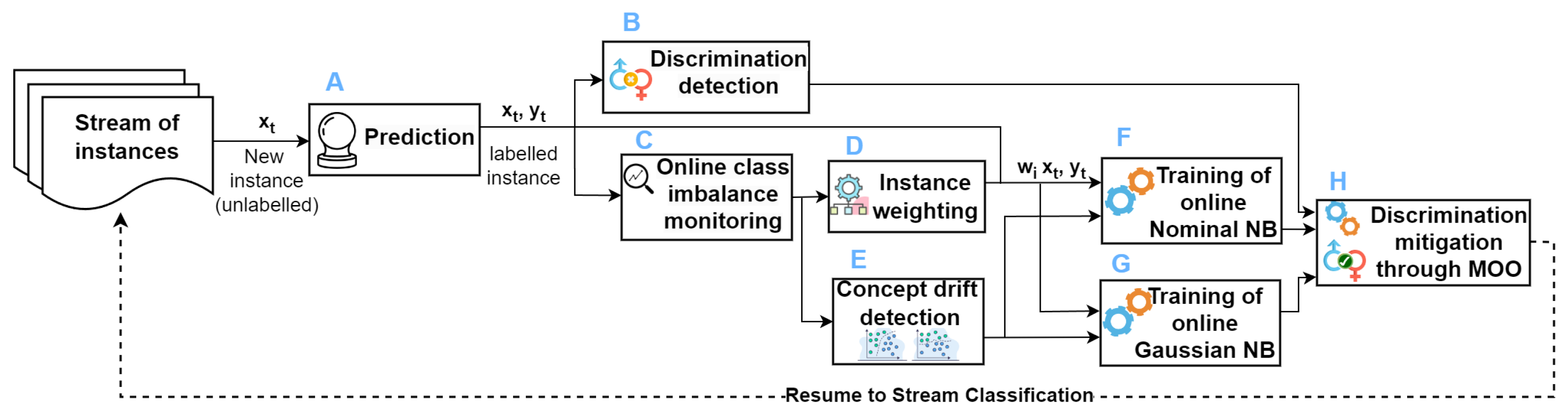
To incorporate causal fairness, we calculate potential outcomes using a matching technique. The objective is to compute the potential outcomes by finding the matched neighbors from the opposite group. For instance, in loan approval, the counterfactual outcome for a female $x_k$ as if she were a male is based on similar males’ observed outcomes. To determine similarity between individuals $x_j$ and $x_k$, we use Propensity Score Matching (PSM) [45]. PSM is aimed at estimating the effect of a treatment by accounting for the covariates that predict receiving the treatment. The propensity score, $e\left(x_k\right)$, is the probability of receiving the treatment given observed covariates (the sensitive attributes (e.g., “gender”) are unlikely to be influenced by any covariates). For the loan approval example, $S_k=1$ denotes the individual k who received the treatment, i.e., the individual is female and $S_k=0$ otherwise. Propensity score of $x_k$ derived from observed covariates $C_k$ is:

$$e\left(x_k\right)=\mathbb{P}(S_k=1|C_k).$$

(5)

The similarity between individuals $x_j$ and $x_k$ is determined through their propensity score difference. The logit version of this difference helps in reducing bias [46]:

$$Diff(j,k)=|logit\left(e\left(x_j\right)\right)-logit\left(e\left(x_k\right)\right)|.$$

(6)

We match treated (protected) and control (non-protected) individuals using nearest neighbor matching with replacement, based on the aforementioned similarity metric.

4. Proposed Model

An illustration of the proposed model is shown in Figure 1. In this study, we are using prequential evaluation with sliding windows; therefore, as soon as a new instance $x_t$ arrives, it is tested using the proposed model (A). After testing, the instance $x_t$ with its true class label $y_t$ is fed to the discrimination detector (B) and online class imbalance monitor OCIM (C). The OCIM monitors the ratios of positive and negative classes throughout the stream and feeds the respective class ratios to the instance weighting module (D). The instance weighting module adjusts the instance weight ($w_i$) in accordance with the respective class ratio to ensure class imbalance-aware learning of the proposed model. The class ratios obtained from the OCIM are also used to keep track of the concept drifts using a concept drift detector (E) and to handle concept recurrence. The instance $x_t$, its true label $y_t$, and the respective weight $w_i$ are used to train online nominal Naïve Bayes (F) and online Gaussian Naïve Bayes (G). The discrimination detector monitors the discrimination over the stream using the employed fairness notion (cumulative statistical parity or cumulative FACE) and triggers the MOO-based discrimination mitigation module (H) if the cumulative discrimination value exceeds a user-defined threshold $\epsilon$. The value of $\epsilon$ depends on the fairness budget allowed by the user, i.e., how much discrimination in predictions is acceptable to the user. We set this value to $0.00001$, which means that we limit our learner to keep the discrimination score in the range [−0.001%, 0.001%].

Further details about these modules are provided in the following subsections.

4.1. Mixed Naïve Bayes

In this work, we tailor the Naïve Bayes algorithm to process streaming data for which we do not have access to historical data. By default, Naïve Bayes is designed only for nominal data. However, in real life, datasets are usually a combination of nominal and continuous attributes. To accommodate continuous and nominal attributes, we propose Mixed Naïve Bayes (MNB), a combination of online nominal Naïve Bayes and online Gaussian Naïve Bayes. For each new instance, continuous attribute values are sent to online Gaussian Naïve Bayes and nominal attribute values are passed to online nominal Naïve Bayes. Online nominal Naïve Bayes and online Gaussian Naïve Bayes update independently. The following sections illustrate the algorithmic details of these two models.

4.1.1. Online Nominal Naïve Bayes

The proposed model is designed for binary classification only. Online nominal Naïve Bayes maintains a summary for each class that contains the count of unique values of each nominal attribute. Whenever a new instance arrives, the summary is updated for the class to which the instance belongs. Since we are using prequential evaluation, the online nominal Naïve Bayes model computes the posterior probabilities of each class with the arrival of each new instance using Equation (7) before updating the summaries.

$$P(C\mid a_1,a_2,a_3,\dots ,a_n)\sim P\left(C\right)\prod _{i=1}^{n}P(a_i\mid C)$$

(7)

4.1.2. Online Gaussian Naïve Bayes

Online Gaussian Naïve Bayes maintains the running mean and variance of each continuous attribute. For this purpose, we use Welford’s online algorithm [47]. The running mean of each attribute is computed using Equation (8). Here, $\overline{a_n}$ is the current mean of the attribute, n is the number of instances, ${\overline{a}}_{n-1}$ is the previous mean, and $a_n$ is the current value of the attribute. To calculate the variance, we need to calculate an intermediate term $M_{2,n}$ as shown in Equation (9). Once we have $M_{2,n}$, we can determine the running variance by Equation (10). With the arrival of every new instance in the stream, the online Gaussian Naïve Bayes updates each continuous attribute’s running mean and variance. The summaries of continuous attributes contain the running mean and variance of the respective attribute.

$$\overline{a_n}=\frac{(n-1){\overline{a}}_{n-1}+a_n}{n}$$

(8)

$$M_{2,n}=M_{2,n-1}+(a_n-{\overline{a}}_{n-1})(a_n-\overline{a_n})$$

(9)

$${\sigma }_n^2=\frac{M_{2,n}}{n}$$

(10)

As we are using prequential evaluation, the online Gaussian Naïve Bayes model computes the posterior probability of each class using Equation (10) before updating the running mean and variance. The only difference is in computing the likelihood of each attribute $a_i$, which is calculated using the following equation:

$$P(a_i\mid C)=\frac{1}{{\sigma }_n\sqrt{2\pi }}exp\left(-\frac{(a_n-\overline{a_n})}{2{\sigma }_n^2}\right).$$

(11)

In the next sections, we describe the details of the modules we propose to handle class imbalance and discrimination in data streams.

4.2. Module for Monitoring and Handling Class Imbalance

We use a class imbalance monitoring component that tracks the proportion of each class in the stream. The roles of majority and minority classes may swap as the stream evolves, i.e., a class that is in the minority at the current time may turn out to be the majority at a later time. We track the state of disequilibrium using the Online Class Imbalance Monitor (OCIM) [48] as shown in Equation (12). In this equation, $C{P}_t^{+}$ is the percentage of positive class at time t and $C{P}_t^{-}$ is the percentage of negative class at time t. After the arrival of each new record, OCIM updates the percentage $C{P}_t$ of the respective class using Equation (13).

$$OCI{M}_t=C{P}_t^{+}-C{P}_t^{-}$$

(12)

$$C{P}_t^y=\alpha ·C{P}_{t-1}^y+(1-\alpha )·\mathbb{I}[y,y_t]$$

(13)

The state of imbalance needs to be changed based on the most recent examples from the stream, and the impact of previous examples needs to be reduced. Therefore, we include a temporal decay factor $(0<\alpha <1)$ to quickly capture the change in disequilibrium. This decay factor limits the impact of historical data; therefore, $C{P}_t^y$ is adjusted based on the most recent records. $\alpha =0$ means that the historical data do not influence the $C{P}_t^y$ at all, and if we keep $\alpha =1$, then we include the complete effect of historical data on $C{P}_t$.$\mathbb{I}[y,y_t]$ is the identity function that returns the value ‘1’ if the predicted label ($y_t$) and the true label (y) are the same; otherwise, it returns the value ‘0’.

Once we have the class percentages (i.e., $C{P}_t^{+}$, $C{P}_t^{-}$), we can use them to find an appropriate weight for each new instance of the data stream. Algorithm 1 presents the complete methodology for computing the instance weights. $C{W}^{+}$ and $C{W}^{-}$ are the class weights of the positive and the negative class, respectively. We compute $C{W}^{+}$ and $C{W}^{-}$ using the class weights library of Sklearn (https://scikit-learn.org, accessed on 22 September 2023). This weighting procedure assigns higher weights to minority class instances than majority class instances. The resulting weight distribution makes the minority class (positive class) more prominent during the training of the learner.

Algorithm 1 Computing instance weights
Require: true class labels y, positive class weight $C{W}^{+}$, negative class weight $C{W}^{-}$, $OCI{M}_t$
1:	Initialize: current instance’s weight $w_i=1$;
2:	if $y==negativelabel$ and $OCI{M}_t>0$ then
3:	$w_i=C{W}^{-}/(1-OCI{M}_t)$
4:	if $y==positivelabel$ and $OCI{M}_t<0$ then
5:	$w_i=C{W}^{+}/(1+OCI{M}_t)$

4.3. Module for Handling Concept Recurrence

As shown in Figure 1, we use a concept drift detector proposed by the Page-Hinkley [49] explicit drift detection method. Our concept drift detection method monitors the OCIM parameter. This method of drift detection works by comparing the current OCIM to $OCIM\_mea{n}_t$. $OCIM\_mea{n}_t$ is the mean value of the OCIM computed for a window of instances up to the current time as illustrated in Equation (14). We chose a window of 1000 instances to compute $OCIM\_mea{n}_t$. In general, concept drift is detected when the observed $OCI{M}_t$ is above the mean $OCIM\_mea{n}_t$ by a specified threshold $\eta$ at a given point in time. Through grid search, we chose the value of $\eta$ as $0.02$. This value of $\eta$ gave us the best discrimination score and predictive performance. With $\eta =0$, concept drift is detected when the mean class imbalance exceeds 0%. Furthermore, $\eta =0.02$ allows the mean class imbalance to be in the range [−2%, 2%].

$$OCIM\_mea{n}_t=\frac{{\sum }_{i=1}^{N}OCI{M}_i}{N}$$

(14)

Concept recurrence is a special case of concept drift where the concepts which have already been seen in the past reappear in the evolving stream. As soon as concept drift is detected, the MNB stores the summaries of next instances as a separate model. In the future, when a similar concept reoccurs (similar concept drift recurs), then MNB retrieves the corresponding model and uses it for further prequential evaluation.

4.4. Online Discrimination Detection and Mitigation

We need to handle discrimination embedded in data streams. As the streams progress, the discriminated groups and the preferred groups do not remain the same. The group that was once discriminated against may turn out to be a preferred group later. Therefore, we need to develop a method that efficiently deals with this concept deviation. Also, we need to maintain the methodology that we developed to deal with the class imbalance problem.

Algorithm 2 illustrates our online discrimination mitigation procedure. To eliminate the discrimination, we change the probability distributions of the protected group $P(S^{-}\mid class)$ and the non-protected group $P(S^{+}\mid class)$ after the arrival of each new example in the data stream. If the discrimination value is greater than a certain threshold $\epsilon$, we add a factor ($\lambda$) of the number of samples belonging to the negative class with protected value N($C_{-},S^{-}$) to the number of samples belonging to the positive class with protected value N($C_{+},S^{-}$) (Algorithm 2: line 2). To avoid unnecessary data augmentation, we also subtract the same factor ($\lambda$) from the number of samples belonging to the negative class with protected value N($C_{-},S^{-}$) (Algorithm 2: lines 3).

Similarly, we add a factor ($\lambda$) of the number of samples belonging to the positive class with non-protected value N($C_{+},S^{+}$) to the number of samples belonging to the negative class with non-protected value N($C_{-},S^{+}$) (Algorithm 2: lines 4). We also subtract the same factor ($\lambda$) from the number of samples belonging to the negative class with the protected value N($C_{+},S^{+}$) (Algorithm 2: lines 5). $\lambda$ is actively tuned through MOO; the details can be found in the next section.

Since we want to deal with concept deviations in the evolving data streams, we also consider negative discrimination, i.e., when the learner starts discriminating against the samples with non-protected value. To remove the negative discrimination, we use the same method as described above, except that now we swap the roles of protected and non-protected groups (Algorithm 2: lines 6 to 10).

Algorithm 2 Online discrimination mitigation procedure.
Require: Summaries of the number of samples belonging to the positive class with protected value N($C_{+},S^{-}$); the number of samples belonging to the positive class with non-protected value N($C_{+},S^{+}$); the number of samples belonging to the negative class with protected value N($C_{-},S^{-}$); the number of samples belonging to the negative class with non-protected value N($C_{-},S^{+}$); discrimination score disc.
Ensure: The overall number of samples does not change.
1:	if $disc>\epsilon$ then
2:	$N(C_{+},S^{-})=N(C_{+},S^{-})+\lambda N(C_{-},S^{-})$
3:	$N(C_{-},S^{-})=N(C_{-},S^{-})-\lambda N(C_{-},S^{-})$
4:	$N(C_{-},S^{+})=N(C_{-},S^{+})+\lambda N(C_{+},S^{+})$
5:	$N(C_{+},S^{+})=N(C_{+},S^{+})-\lambda N(C_{+},S^{+})$
6:	if $disc<-\epsilon$ then
7:	$N(C_{+},S^{+})=N(C_{+},S^{+})+\lambda N(C_{-},S^{+})$
8:	$N(C_{-},S^{+})=N(C_{-},S^{+})-\lambda N(C_{-},S^{+})$
9:	$N(C_{-},S^{-})=N(C_{-},S^{-})+\lambda N(C_{+},S^{-})$
10:	$N(C_{+},S^{-})=N(C_{+},S^{-})-\lambda N(C_{+},S^{-})$

Adaptive Hyperparameter Tuning through MOO

In our research, we employ the Non-dominated Sorting Genetic Algorithm II (NSGA-II) [50] as a multi-objective optimization (MOO) method, to actively tune the hyperparameter $\lambda$ during windowed prequential evaluation of streaming data to simultaneously optimize our multiple objectives, i.e., balanced accuracy and fairness. This MOO-based method assists in selecting a $\lambda$ that reduces discrimination as well as not only retaining but also enhancing the benefits obtained by the class imbalance handling module, i.e., the high predictive performance. For every window of n instances, the MOO procedure, outlined in Algorithm 3, is invoked to optimize $\lambda$ based on a trade-off between balanced accuracy and discrimination score. In each invocation, a population of M values of $\lambda$ is initialized (Algorithm 3: line 1). The parent and child populations of $\lambda$ are merged to form ${\lambda }_h^g$ (Algorithm 3: line 3). Each lambda in this merged population is then used to test (windowed prequential evaluation) Fair-CMNB and the corresponding solutions (pairs of balanced accuracy and discrimination scores) are found (Algorithm 3: line 4). The Pareto front represents the set of optimal trade-offs between the two objectives, i.e., balanced accuracy and discrimination score; each point on the Pareto front ($[B.Acc.,disc\_score]$) signifies a unique balance between the balanced accuracy and discrimination score. Some points may have a high discrimination score but lower balanced accuracy, and others may have high balanced accuracy but a lower discrimination score. Fast non-dominated sorting is then applied to sort the Pareto fronts $\mathcal{P}$ (Algorithm 3: line 5). The next generation’s parent population (${\lambda }_p^{g+1}$) is incrementally populated by including individuals from the sorted fronts, up to a size limit of M. Crowding distance is calculated within each front (${\mathcal{P}}^j$) to preserve diversity among the solutions (Algorithm 3: lines 7 to 11). The newly found Pareto fronts are sorted based on their dominance to determine their inclusion priority in the subsequent generation (Algorithm 3: line 12). Only the first ($M-|{\lambda }_p^{g+1}|$) elements of the final (${\mathcal{P}}^j$) are added to the parent population (Algorithm 3: line 13) to keep the size of the population intact, i.e., M. The child population for the next generation (${\lambda }_c^{g+1}$) is formed using selection, crossover, and mutation operations on the newly formed parent population (Algorithm 3: line 14). After completing a generation, the generation counter g is incremented. This optimization process stops if we reach the maximum number of generations Z or the trade-off value (Equation (15)) is not improving over a fixed number of previous generations; the algorithm sorts the final child population by the trade-off criterion to select the optimal $\lambda$ value (${\lambda }_{\mathrm{best}}$) (Algorithm 3: lines 15 to 16). This trade-off measure is inspired by F-score, where $\mu$ is a hyperparameter that makes the discrimination score (disc_score) $\mu$ times more important than the balanced accuracy (B.Acc.). If we keep the value of $\mu$ equal to 1, then the trade-off becomes the harmonic mean between B.Acc. and $1-\mathit{abs}(\mathit{disc}\_\mathit{score})$. The selected ${\lambda }_{best}$ is then used for the windowed prequential evaluation of the subsequent t instances, after which the MOO procedure is invoked again.

$$\mathrm{trade-off}=(1+{\mu }^2) \ast \left(\frac{\mathit{B}.\mathit{Acc}. \ast (1-\mathit{abs}(\mathit{disc}\_\mathit{score}\left)\right)}{\mu \ast \mathit{B}.\mathit{Acc}. + (1-\mathit{abs}(\mathit{disc}\_\mathit{score}\left)\right)}\right)$$

(15)

Algorithm 3 Multi-objective optimization procedure to actively tune $\lambda$.
Require: Summaries of all the samples of a window
Ensure: Optimized $\lambda$ to ensure Pareto optimal trade-off between balanced accuracy and discrimination score.
1:	${\lambda }_c^g=init(size=M),g=1,{\lambda }_c^g=\varphi$
2:	while $g\le Z$ or trade-off improving do
3:	${\lambda }_h^g={\lambda }_p^g\cup {\lambda }_c^g$                                                                                         ▹ Combine parent and child populations of $\lambda$
4:	${\mathcal{Y}}_h={[B.Acc.,disc\_score]}_{i=1}^n=Fair-CMNB.preq\_eval\left({\lambda }_h^g\right)$
5:	$\mathcal{P}=fast\_non\_dominated\_sort\left({\mathcal{Y}}_h\right)$                                                            ▹ sorted non dominated fronts of ${\lambda }_h$
6:	${\lambda }_p^{g+1}=\varphi ,j=1$
7:	repeat
8:	$crowding\_distance\_computation\left({\mathcal{P}}^j\right)$
9:	${\lambda }_p^{g+1}={\lambda }_p^{g+1}\cup {\mathcal{P}}^j$
10:	$j=j+1$
11:	until $|{\lambda }_p^{g+1}|+|{\mathcal{P}}^j|\le M$
12:	$sort\_by\_dominance\left({\mathcal{P}}^j\right)$                                                  ▹ sort ${\mathcal{P}}^j$ in descending order according to dominance
13:	${\lambda }_p^{g+1}={\lambda }_p^{g+1}\cup {\mathcal{P}}^j[1:(M-|{\lambda }_p^{g+1}\left|\right)]$
14:	${\lambda }_c^{g+1}=make\_new\_population\left({\lambda }_p^{g+1}\right)$▹ make new/ child population using selection, crossover, and mutation
15:	$g=g+1$
16:	${\lambda }_{best}=sort\_and\_select\_best\_by\_\mathit{trade-off}\left({\lambda }_c\right)$

5. Complexity Analysis

5.1. Online Naïve Bayes Classifier

• Model Update: For d features and c classes, the update complexity is $\mathcal{O}\left(dc\right)$.
• Prediction: The prediction complexity per data point is $\mathcal{O}\left(dc\right)$.

5.2. NSGA-II for Hyperparameter Tuning

• Population Initialization: Time complexity for initial population setup with p individuals is $\mathcal{O}\left(p\right)$.
• Fitness Evaluation: For p individuals, with E as the evaluation time, the complexity is $\mathcal{O}\left(pE\right)$.
• Non-dominated Sorting and Selection: The sorting process complexity is $\mathcal{O}\left(p^2\right)$.
• Genetic Operators: The complexity of crossover and mutation operations is $\mathcal{O}\left(p\right)$.

5.3. Page-Hinkley for Concept Drift Detection

• Drift Detection: The complexity for each incoming data point is $\mathcal{O}\left(1\right)$.

5.4. Overall Computational Complexity

Assuming N total data points and hyperparameter tuning every T time steps:

• Online Naïve Bayes: Update and Prediction complexity is $\mathcal{O}\left(Ndc\right)$.
• NSGA-II Operations: Dominated by the fitness evaluation, it is $\mathcal{O}(pE+p^2+p)$, primarily $\mathcal{O}\left(pE\right)$.
• Page-Hinkley Drift Detection: Overall complexity is $\mathcal{O}\left(N\right)$.

The overall complexity is dominated by the most expensive operation among these, typically the hyperparameter tuning cost $\mathcal{O}\left(pE\right)$, if significant.

6. Evaluation Setup

6.1. Benchmark Baselines

We compare the proposed methodology against five baseline models including the class imbalance-aware CSMOTE [40], non-stationary OSBoost [28], fairness-agnostic massaging (MS) [34], fairness-aware FAHT [35], and class imbalance- and discrimination-aware FABBOO [1]. All the baselines are trained using the same hyperparameters as given in the respective research articles. We also evaluate different variants of MNB to stress the effectiveness of different modules of the proposed model.

• CSMOTE [40]: This baseline is not fairness-aware, but it is designed to handle class imbalance in a non-stationary environment by re-sampling the minority class in a defined window of instances.
• OSBoost [28]: This is a classification model for data streams. It is not capable of handling either class imbalance or discrimination.
• Massaging (MS) [34]: This is a fairness-aware learning method. It is a chunk-based technique which handles discrimination in the current chunk by swapping labels. But it does not account for cumulative effects of discrimination; it is designed to handle discrimination only on a short-term basis, i.e., for the current chunk. We use the default chunk size for training this baseline, i.e., 1000, as proposed by [34]. This method cannot handle class imbalance.
• Fairness-Aware Hoeffding Tree (FAHT) [35]: This method is an adaptation of Hoeffding tree that is designed to deal with discrimination. It incorporates the fairness gain along with the information gain into the partitioning criteria of the decision tree. This model is not able to deal with class imbalance and concept drifts.
• FABBOO [1]: This is an online boosting approach that handles class imbalance by monitoring class ratios in an online fashion. It employs boundary adjustment methods to handle discrimination.
• MNB (Mixed Naïve Bayes): This is a combination of online nominal Naïve Bayes and online Gaussian Naïve Bayes. It considers no notion of fairness and class imbalance while performing classification tasks.
• Fair-CMNB (Discrimination- and Class Imbalance-Aware Mixed Naïve Bayes): This is a variant of MNB which mitigates discrimination (utilizing MOO) as well as handles class imbalance and concept drifts in the evolving stream.

6.2. Benchmark Datasets

The details of the datasets used to test the efficiency of the proposed model are shown in

Table 1. Description of datasets.

Dataset	#Inst.	#Att.	Sens. Att.	Class Imb.	Positive Class	Type
Adult Census [51]	45,175	14	Gender	1:3.0	>50 K	Static
Compas [52]	5278	9	Race	1:1.1	recidivism	Static
KDD [51]	299,285	41	Gender	1:15.1	>50 K	Static
Default [51]	30,000	24	Gender	1:3.52	default payment	Static
Law School [53]	18,692	12	Gender	1:3.5	pass bar	Static
NYPD [54]	311,367	16	Gender	1:3.7	felony	Stream
Loan [55]	21,443	38	Gender	1:1.26	paid	Stream
Bank Marketing [51]	41,188	21	Marital Status	1:7.87	subscription	Stream

. The datasets have different characteristics related to the number of attributes (#Att.), number of instances (#Inst.), sensitive attribute (Sens. Att.), and class ratio (positive to negative). We are using static datasets along with the streaming datasets. Despite the growing interest in AI models that focus on fairness, there is still a lack of large streaming datasets in this domain. Therefore, we use static datasets along with streaming datasets to prove the effectiveness of our proposed model. Since we are unaware of the temporal characteristics of the static datasets, we report the evaluation metrics on the average of 10 random shuffles of each static dataset that passes through the model.

6.3. Evaluation Metrics

We use recall, balanced accuracy, gmean, cumulative statistical parity (St. Parity), and cumulative FACE to measure the predictive and fairness performance of the proposed framework and competing baselines. The mathematical representation of recall, balanced accuracy, and gmean are illustrated in Equations (16), (18), and (19). The details of statistical parity and FACE have already been explained in Section 3.3.

$$Recall=\frac{TP}{TP+FN}$$

(16)

$$Specificity=\frac{TN}{TN+FP}$$

(17)

$$BalancedAccuracy=\frac{Recall+Specificity}{2}$$

(18)

$$Gmean=\sqrt{Recall \ast Specificity}$$

(19)

7. Results and Discussion

The proposed models are trained and tested following the prequential evaluation with sliding windows (with a window size of 1000 instances) strategy, i.e., test first, then train. We tune the hyperparameters $\alpha$ and $ϵ$ by grid search. To obtain the best results for all datasets, we choose values of $0.9$ and $0.00001$ for $\alpha$ and $ϵ$, respectively. As mentioned earlier, the non-streaming datasets lack temporal features; therefore, we use ten random shuffles of each static dataset and present the average of their results. All the baselines are also evaluated using the prequential evaluation with sliding windows method.

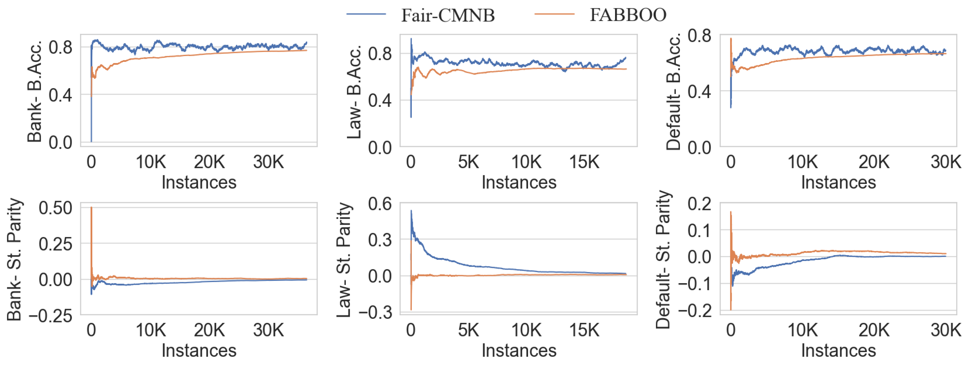
7.1. Comparison with Baselines

Table 2. Comparison of fairness and predictive performance achieved by Fair-CMNB and the competing baselines for streaming datasets with windowed prequential evaluation; best and second-best results are in bold and underline, respectively.

Dataset	Model	Recall (%)	B.Acc. (%)	Gmean (%)	St. Parity (%)
NYPD	CSMOTE	98.01	58.19	42.43	4.82
	OSBoost	98.87	52.20	23.38	−0.60
	MS	19.17	58.94	43.50	6.39
	FAHT	0.45	49.01	6.62	0.06
	FABBOO	48.73	64.15	71.44	0.03
	Fair-CMNB	86.78	81.25	81.06	0.019
Bank Marketing	CSMOTE	85.91	83.21	83.16	7.34
	OSBoost	37.65	68.55	61.19	2.93
	MS	35.29	66.43	58.67	6.68
	FAHT	38.15	67.95	61.06	2.07
	FABBOO	57.03	76.16	73.71	1.02
	Fair-CMNB	82.91	82.06	82.05	−0.033
Loan	CSMOTE	75.57	71.64	71.53	2.88
	OSBoost	78.61	69.61	69.02	4.72
	MS	69.00	68.53	68.52	50.83
	FAHT	69.41	68.01	67.99	0.12
	FABBOO	75.60	69.67	69.41	0.75
	Fair-CMNB	86.25	80.37	79.87	0.065

presents the measures of fairness and predictive performance obtained by the proposed model (Fair-CMNB) and the competing baselines for a set of streaming datasets. Similarly, the evaluation measures obtained on the average of 10 random shuffles of each static dataset by Fair-CMNB and the baselines are shown in

Table 3. Comparison of fairness and predictive performance achieved by Fair-CMNB and the competing baselines for static datasets with windowed prequential evaluation; best and second-best results are in bold and underline, respectively.

Dataset	Model	Recall (%)	B.Acc. (%)	Gmean (%)	St. Parity (%)
Adult Census	CSMOTE	81.92	79.73	79.69	29.88
	OSBoost	56.06	73.85	71.67	19.19
	MS	51.98	74.32	70.88	23.54
	FAHT	51.36	75.23	71.34	16.18
	FABBOO	66.26	75.90	75.28	0.25
	Fair-CMNB	84.56	81.24	81.17	0.0227
KDD	CSMOTE	65.17	76.77	75.88	9.36
	OSBoost	33.61	66.35	57.71	5.15
	MS	27.88	63.44	52.53	15.80
	FAHT	29.65	63.92	53.95	2.44
	FABBOO	78.39	81.97	81.89	0.17
	Fair-CMNB	88.01	84.11	82.13	0.026
Compas	CSMOTE	66.12	67.05	67.04	20.19
	OSBoost	61.09	67.11	66.83	25.99
	MS	60.26	65.38	65.17	45.02
	FAHT	62.25	65.21	66.69	21.43
	FABBOO	65.06	65.15	65.14	1.03
	Fair-CMNB	70.40	71.71	71.69	0.776
Default	CSMOTE	81.69	60.80	57.09	3.21
	OSBoost	32.88	64.09	55.97	1.97
	MS	32.27	63.97	55.56	10.28
	FAHT	31.92	64.93	55.91	1.62
	FABBOO	43.19	66.14	62.03	0.79
	Fair-CMNB	62.23	69.63	69.23	0.012
Law School	CSMOTE	76.01	75.27	74.53	1.43
	OSBoost	18.96	59.12	43.38	1.29
	MS	19.07	58.87	43.38	3.23
	FAHT	14.49	55.61	37.43	0.76
	FABBOO	40.48	69.21	62.97	0.27
	Fair-CMNB	74.25	81.27	80.97	0.012

. From Table 2 and Table 3, we can observe that we always achieve the best discrimination score (St. Parity) as compared to all the baselines. Compared to SoTA methods, Fair-CMNB achieves the best balanced accuracy for the Adult Census, KDD, Default, Law School, NYPD, and Loan datasets. Although CSMOTE is a class imbalance-aware baseline, Fair-CMNB outperforms it in terms of balanced accuracy for all datasets except the Bank Marketing dataset. For the Bank Marketing dataset, CSMOTE (baselines model without fairness interventions) reports the best balanced accuracy but Fair-CMNB follows it with a close margin of $1.15\%$. However, the difference between the discrimination score achieved by CSMOTE and the proposed model for the Marketing dataset is substantial, i.e., $7.373\%$.

There is a noticeable disparity between the recall and balanced accuracy values obtained by fairness-aware baselines: MS, FAHT, and FABBOO. This suggests that these baselines attempt to alleviate discrimination by significantly sacrificing either the true positive rate or the true negative rate. In contrast, for most datasets, Fair-CMNB delivers recall and balanced accuracy values that are closely aligned.

Our research question is closely related to that of FABBOO. The predictive performance and discrimination scores achieved by Fair-CMNB are much better than those of FABBOO for both streaming and static datasets. We can observe that Fair-CMNB achieved $3.32\%$, $2.14\%$, $6.56\%$, $3.23\%$, $12.06\%$, $17.1\%$, $5.9\%$, and $10.7\%$ higher balanced accuracy values for the Adult Census, KDD, Compas, Default, Law School, NYPD, Bank Marketing, and Loan datasets as compared to those achieved by FABBOO while maintaining low discrimination scores. A similar trend can be observed for gmean.

FABBOO has the capability to reduce discrimination score to a suitable value while maintaining balanced accuracy but it is not able to handle negative discrimination. Also, FABBOO reports a significant difference in recall and balanced accuracy which indicates that it is achieving a low discrimination score at the cost of ignoring either the minority or the majority class. For example, for the Default dataset we observe a difference of $22.95\%$ between recall and balanced accuracy reported by FABBOO. However, Fair-CMNB reports only a difference of $7.4\%$ between recall and balanced accuracy. This proves that FABBOO struggles to handle class imbalance while mitigating discrimination. Similar behavior can be observed for other imbalanced as well as balanced datasets, i.e., Adult Census, Law School, Bank Marketing, NYPD, and Loan.

Figure 2 presents a comparison of the balanced accuracy and statistical parity values attained by Fair-CMNB and FABBOO for the Bank Marketing, Law School, and Default datasets. From this figure, it is evident that while both Fair-CMNB and FABBOO achieve similar statistical parity scores, Fair-CMNB consistently outperforms FABBOO in terms of balanced accuracy throughout the stream for all datasets.

7.2. Scalability

Fair-CMNB adapts well to large data volumes. Law School is the smallest dataset with approximately 18,000 instances, while KDD and NYPD are much larger, with each containing around 300,000 instances. As is evident from Table 2 and Table 3, Fair-CMNB’s performance remains consistent across both small (Law School) and large (KDD, NYPD) datasets. This demonstrates Fair-CMNB’s efficient scalability with increasing data volume.

7.3. Agnosticism to Fairness Notions

We are using windowed prequential evaluation; therefore, we have access to the most recent window of instances. We generate the potential outcomes for this window of instances using the method mentioned in Section 3.4 and determine the FACE value. The predictive and fairness performance measures obtained by Fair-CMNB under causal fairness notion are presented in

Table 4. Fairness and predictive performance of Fair-CMNB under causal fairness notion. Fair-CMNB achieves high predictive performance along with very low FACE values, demonstrating its adaptability to different fairness notions.

Dataset	Recall (%)	B.Acc. (%)	Gmean (%)	FACE (%)
Adult Census	85.55	80.56	80.41	0.488
KDD	86.96	82.61	82.50	−0.104
Compas	77.94	70.53	70.13	0.346
Default	63.39	69.23	68.98	−0.131
Law School	71.84	77.77	77.54	−0.028
NYPD	76.85	78.34	78.33	0.066
Bank Marketing	79.95	80.63	80.61	0.929
Loan	93.95	87.59	87.35	0.812

. The results indicate that Fair-CMNB consistently achieves high balanced accuracy alongside remarkably low FACE values across all datasets. This underscores Fair-CMNB’s agnosticism to the specific fairness notion in use.

7.4. Impact Assessment of Naïve Bayes Modules

In this section, we compare the predictive and fairness performance of MNB (without fairness interventions) and Fair-CMNB (with fairness interventions) as shown in

Table 5. Comparison of fairness and predictive performance among MNB variants. Results show that Fair-CMNB effectively reduces discrimination while simultaneously enhancing predictive accuracy.

Dataset	Model	Recall (%)	B.Acc. (%)	Gmean (%)	St. Parity (%)
Adult Census	MNB	78.15	79.79	79.77	29.17
	Fair-CMNB	84.56	81.24	81.17	0.0227
KDD	MNB	78.03	82.17	82.06	14.35
	Fair-CMNB	88.01	84.11	82.13	0.026
Compas	MNB	67.85	68.96	68.95	27.28
	Fair-CMNB	70.40	71.71	71.69	0.776
Default	MNB	52.04	68.46	66.46	2.65
	Fair-CMNB	62.23	69.63	69.23	0.012
Law School	MNB	86.51	76.13	75.41	49.64
	Fair-CMNB	74.25	81.27	80.97	0.012
NYPD	MNB	71.76	76.43	76.28	19.85
	Fair-CMNB	86.78	81.25	81.06	0.019
Bank Marketing	MNB	71.31	79.51	79.08	2.71
	Fair-CMNB	82.91	82.06	82.05	−0.033
Loan	MNB	82.00	77.35	77.2	14.73
	Fair-CMNB	89.25	80.37	79.87	0.065

. From the results, we can observe that Fair-CMNB effectively reduces discrimination (St. Parity) while simultaneously improving the predictive performance. Specifically, for datasets such as Adult Census, KDD, Compas, Default, Law School, NYPD, Bank Marketing, and Loan, Fair-CMNB reduces discrimination (St. Parity) from $29.17\%$ to $0.0227\%$, $14.35\%$ to $0.026\%$, $27.28\%$ to $0.776\%$, $2.65\%$ to $0.012\%$, $49.64\%$ to $0.012\%$, $19.85\%$ to $0.019\%$, $2.71\%$ to $-0.033\%$, and $14.73\%$ to $0.065\%$, respectively. Concurrently, while diminishing St. Parity, Fair-CMNB enhances the predictive performance across all datasets, underscoring the effectiveness of our MOO-based approach. Notably, our technique ensures parity between protected and non-protected groups, evident even in balanced datasets like Compas and Loan.

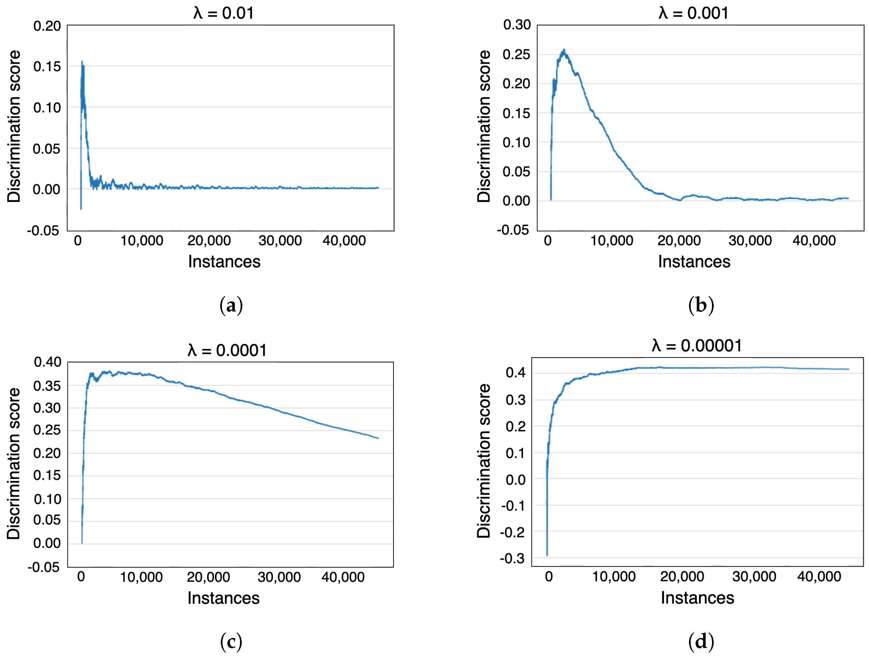
7.5. Hyperparameter Sensitivity

The most important hyperparameter in reducing discrimination is $\lambda$ from Algorithm 2. We examined the effect of changing $\lambda$ on the ability of our proposed model to reduce discrimination, as shown in Figure 3. We used the Adult Census dataset as a reference for this analysis. As can be seen in Figure 3a, when the value of $\lambda$ is $0.01$, the discrimination value immediately drops to zero, indicating that this value is too large. With this value of $\lambda$, we achieve a balanced accuracy of $75.13\%$. If we decrease $\lambda$ to a value of $0.001$, the discrimination score decreases to a smaller and stable value after about 20,000 instances, as shown in Figure 3b. The balanced accuracy is also not much affected with a value of $78.61\%$. If we further decrease the value of $\lambda$ to $0.0001$, the discrimination score does not reach a stable value until the end of the stream, although it decreases as shown in Figure 3c. This value of $\lambda$ leads to a balanced accuracy of $79.93\%$. As shown in Figure 3d, if we leave $\lambda$ at $0.00001$, the discrimination score does not decrease throughout the data stream, and the achieved balanced accuracy is $80.37\%$. Therefore, we chose the value $0.001$ for $\lambda$, which provides a good trade-off between the balanced accuracy and the attenuation of the discrimination score.

7.6. Deep Learning vs. Naïve Bayes

Deep neural networks (DNNs) can be computationally intensive due to their inherent structure and the iterative nature of their training process. On the other hand, Naïve Bayes, being based on straightforward probabilistic computations, is generally faster and more scalable. We evaluated the runtime of a four-layer online DNN, as proposed by [56], on the Law School dataset with windowed prequential evaluation. Our findings indicate that MNB (without fairness and class imbalance interventions) finished training in $130.624$ s, while Fair-CMNB (with fairness interventions) took $360.183$ s. Meanwhile, the DNN (without fairness and class imbalance interventions) required approximately $627.933$ s to complete its training throughout the entire data stream. All tests were conducted on an Intel Core i7 CPU equipped with 64 GB RAM.

8. Conclusions

The central prerequisite of a just and sustainable world is to ensure gender equality and realize the human rights, nobility, and competence of diverse groups of society. Deep learning, although successful in many domains, may not always be optimal for fairness-aware stream learning where computational efficiency and model interpretability are major concerns. Therefore, we propose a multi-objective optimization (MOO)-based discrimination- and class imbalance-aware online learning framework to achieve parity between favored and prejudiced groups of subjects.

We present a novel adaptation of Naïve Bayes for mining data streams with embedded discrimination and class imbalance. We have demonstrated the effectiveness of our methodology by conducting experiments on a range of static and streaming datasets. Our approach mitigates both discrimination and reverse discrimination by modifying the data distribution based on a cumulative fairness notion through an MOO method. Our approach outperforms existing SoTA methods in terms of both balanced accuracy and discrimination score. We have shown that our approach effectively learns both majority and minority classes and achieves a low discrimination score while maintaining high predictive performance. We have also shown the adaptability of Fair-CMNB to different fairness notions (including the causal fairness notion FACE). To the best of our knowledge, this is the first attempt where a causal fairness notion is used to assess the discriminating behavior of a framework in online settings.

In the future, we aim to thoroughly investigate the forgetting phenomena of the class imbalance handling module to make it adaptable to the nature of concept drift in the data. We also plan to analyze the theoretical aspects of our approach.

References

1. Iosifidis, V.; Ntoutsi, E. FABBOO-Online Fairness-Aware Learning Under Class Imbalance. In Proceedings of the International Conference on Discovery Science, Thessaloniki, Greece, 19–21 October 2020; Springer: Cham, Switzerland, 2020; pp. 159–174. [Google Scholar]
2. Iosifidis, V.; Ntoutsi, E. Dealing with Bias via Data Augmentation in Supervised Learning Scenarios; Bates, J., Clough, P.D., Jäschke, R., Eds.; BibSonomy: Kassel, Germany, 2018; pp. 24–29. [Google Scholar]
3. Aghaei, S.; Azizi, M.J.; Vayanos, P. Learning optimal and fair decision trees for non-discriminative decision-making. In Proceedings of the 2019 AAAI/ACM Conference on AI, Ethics, and Society, Honolulu, HI, USA, 27 January–1 February 2019; Volume 33, pp. 1418–1426. [Google Scholar]
4. Kamiran, F.; Calders, T. Classifying without discriminating. In Proceedings of the Computer, Control and Communication, 2009, IC4 2009, 2nd International Conference, Karachi, Pakistan, 17–18 February 2009; pp. 1–6. [Google Scholar]
5. Kamiran, F.; Calders, T.; Pechenizkiy, M. Discrimination aware decision tree learning. In Proceedings of the 2010 IEEE International Conference on Data Mining, Sydney, NSW, Australia, 13–17 December 2010; pp. 869–874. [Google Scholar]
6. Zafar, M.B.; Valera, I.; Gomez-Rodriguez, M.; Gummadi, K.P. Fairness constraints: A flexible approach for fair classification. J. Mach. Learn. Res. 2019, 20, 2737–2778. [Google Scholar]
7. Liu, A.; Song, Y.; Zhang, G.; Lu, J. Regional concept drift detection and density synchronized drift adaptation. In Proceedings of the Twenty-Sixth International Joint Conference on Artificial Intelligence, Melbourne, Australia, 19–25 August 2017. [Google Scholar]
8. Lelie, F.; Crul, M.; Schneider, J. The European Second Generation Compared: Does the Integration Context Matter; Amsterdam University Press: Amsterdam, The Netherlands, 2012. [Google Scholar]
9. Wang, X.; Zhao, Y.; Pourpanah, F. Recent advances in deep learning. Int. J. Mach. Learn. Cybern. 2020, 11, 747–750. [Google Scholar] [CrossRef]
10. Xhemali, D.; Hinde, C.J.; Stone, R. Naïve bayes vs. decision trees vs. neural networks in the classification of training web pages. IJCSI Int. J. Comput. Sci. Issues 2009, 4, 16–23. [Google Scholar]
11. Khademi, A.; Lee, S.; Foley, D.; Honavar, V. Fairness in algorithmic decision making: An excursion through the lens of causality. In Proceedings of the World Wide Web Conference, San Francisco, CA, USA, 13–17 May 2019; pp. 2907–2914. [Google Scholar]
12. Mehrabi, N.; Morstatter, F.; Saxena, N.; Lerman, K.; Galstyan, A. A survey on bias and fairness in machine learning. ACM Comput. Surv. (CSUR) 2021, 54, 1–35. [Google Scholar] [CrossRef]
13. Calders, T.; Kamiran, F.; Pechenizkiy, M. Building classifiers with independency constraints. In Proceedings of the IEEE International Conference on Data Mining Workshops, Miami, FL, USA, 6 December 2009; pp. 13–18. [Google Scholar]
14. Kamiran, F.; Calders, T. Data preprocessing techniques for classification without discrimination. Knowl. Inf. Syst. 2012, 33, 1–33. [Google Scholar] [CrossRef]
15. Zhang, L.; Wu, Y.; Wu, X. Achieving Non-Discrimination in Prediction. In Proceedings of the Twenty-Seventh International Joint Conference on Artificial Intelligence, Stockholm, Sweden, 13–19 July 2018; pp. 3097–3103. [Google Scholar]
16. Petrović, A.; Nikolić, M.; Radovanović, S.; Delibašić, B.; Jovanović, M. FAIR: Fair adversarial instance re-weighting. Neurocomputing 2022, 476, 14–37. [Google Scholar] [CrossRef]
17. Shekhar, S.; Fields, G.; Ghavamzadeh, M.; Javidi, T. Adaptive sampling for minimax fair classification. Adv. Neural Inf. Process. Syst. 2021, 34, 24535–24544. [Google Scholar]
18. Padala, M.; Gujar, S. FNNC: Achieving fairness through neural networks. In Proceedings of the Twenty-Ninth International Joint Conference on Artificial Intelligence, Yokohama, Japan, 7–15 January 2021. [Google Scholar]
19. Iosifidis, V.; Ntoutsi, E. Adafair: Cumulative fairness adaptive boosting. In Proceedings of the 28th ACM International Conference on Information and Knowledge Management, Beijing, China, 3–7 November 2019; pp. 781–790. [Google Scholar]
20. Blanzeisky, W.; Cunningham, P. Using Pareto simulated annealing to address algorithmic bias in machine learning. Knowl. Eng. Rev. 2022, 37, e5. [Google Scholar] [CrossRef]
21. Calders, T.; Verwer, S. Three naive bayes approaches for discrimination-free classification. Data Min. Knowl. Discov. 2010, 21, 277–292. [Google Scholar] [CrossRef]
22. Hajian, S.; Domingo-Ferrer, J.; Monreale, A.; Pedreschi, D.; Giannotti, F. Discrimination-and privacy-aware patterns. Data Min. Knowl. Discov. 2015, 29, 1733–1782. [Google Scholar] [CrossRef]
23. Fish, B.; Kun, J.; Lelkes, Á.D. A confidence-based approach for balancing fairness and accuracy. In Proceedings of the SIAM International Conference on Data Mining, Miami, FL, USA, 5–7 May 2016; pp. 144–152. [Google Scholar]
24. Nguyen, D.; Gupta, S.; Rana, S.; Shilton, A.; Venkatesh, S. Fairness improvement for black-box classifiers with Gaussian process. Inf. Sci. 2021, 576, 542–556. [Google Scholar] [CrossRef]
25. Chiappa, S. Path-specific counterfactual fairness. In Proceedings of the AAAI Conference on Artificial Intelligence, Hilton, HI, USA, 27 January–1 February 2019; Volume 33, pp. 7801–7808. [Google Scholar]
26. Masud, M.M.; Woolam, C.; Gao, J.; Khan, L.; Han, J.; Hamlen, K.W.; Oza, N.C. Facing the reality of data stream classification: Coping with scarcity of labeled data. Knowl. Inf. Syst. 2012, 33, 213–244. [Google Scholar] [CrossRef]
27. Bifet, A.; Pfahringer, B.; Read, J.; Holmes, G. Efficient data stream classification via probabilistic adaptive windows. In Proceedings of the 28th Annual ACM Symposium on Applied Computing, Coimbra, Portugal, 18–22 March 2013; pp. 801–806. [Google Scholar]
28. Chen, S.T.; Lin, H.T.; Lu, C.J. An online boosting algorithm with theoretical justifications. arXiv 2012, arXiv:1206.6422. [Google Scholar]
29. Yu, H.; Zhang, Q.; Liu, T.; Lu, J.; Wen, Y.; Zhang, G. Meta-ADD: A meta-learning based pre-trained model for concept drift active detection. Inf. Sci. 2022, 608, 996–1009. [Google Scholar] [CrossRef]
30. Nguyen, T.T.T.; Nguyen, T.T.; Sharma, R.; Liew, A.W.C. A lossless online Bayesian classifier. Inf. Sci. 2019, 489, 1–17. [Google Scholar] [CrossRef]
31. Liu, Y.; Xu, Z.; Li, C. Online semi-supervised support vector machine. Inf. Sci. 2018, 439–440, 125–141. [Google Scholar] [CrossRef]
32. Abbasi, A.; Javed, A.R.; Chakraborty, C.; Nebhen, J.; Zehra, W.; Jalil, Z. ElStream: An Ensemble Learning Approach for Concept Drift Detection in Dynamic Social Big Data Stream Learning. IEEE Access 2021, 9, 66408–66419. [Google Scholar] [CrossRef]
33. Paulraj, D.; Prem M, V. A Novel Ensemble Classifier Framework to Preprocess, Learn and Predict Imbalanced Heterogeneous Drifted Data Stream. In Proceedings of the 2023 Second International Conference on Electrical, Electronics, Information and Communication Technologies (ICEEICT), Erode, India, 5–7 April 2023; pp. 1–7. [Google Scholar] [CrossRef]
34. Iosifidis, V.; Tran, T.N.H.; Ntoutsi, E. Fairness-enhancing interventions in stream classification. In Proceedings of the International Conference on Database and Expert Systems Applications, Linz, Austria, 26–29 August 2019; Springer: Cham, Switzerland, 2019; pp. 261–276. [Google Scholar]
35. Zhang, W.; Ntoutsi, E. FAHT: An Adaptive Fairness-aware Decision Tree Classifier. In Proceedings of the Twenty-Eighth International Joint Conference on Artificial Intelligence, Macao, China, 10–16 August 2019; pp. 1480–1486. [Google Scholar]
36. Badar, M.; Nejdl, W.; Fisichella, M. FAC-fed: Federated adaptation for fairness and concept drift aware stream classification. Mach. Learn. 2023, 112, 2761–2786. [Google Scholar] [CrossRef]
37. Pham, D.; Tran, B.; Nguyen, S.; Alahakoon, D. Fairness Aware Swarm-based Machine Learning for Data Streams. In Proceedings of the AI 2022: Advances in Artificial Intelligence, Perth, WA, Australia, 5–8 December 2022; pp. 205–219. [Google Scholar]
38. Thabtah, F.; Hammoud, S.; Kamalov, F.; Gonsalves, A. Data imbalance in classification: Experimental evaluation. Inf. Sci. 2020, 513, 429–441. [Google Scholar] [CrossRef]
39. Wang, B.; Pineau, J. Online bagging and boosting for imbalanced data streams. IEEE Trans. Knowl. Data Eng. 2016, 28, 3353–3366. [Google Scholar] [CrossRef]
40. Bernardo, A.; Gomes, H.M.; Montiel, J.; Pfahringer, B.; Bifet, A.; Della Valle, E. C-SMOTE: Continuous Synthetic Minority Oversampling for Evolving Data Streams. In Proceedings of the 2020 IEEE International Conference on Big Data (Big Data), Atlanta, GA, USA, 10–13 December 2020; pp. 483–492. [Google Scholar]
41. Younis, R.; Fisichella, M. FLY-SMOTE: Re-balancing the non-IID iot edge devices data in federated learning system. IEEE Access 2022, 10, 65092–65102. [Google Scholar] [CrossRef]
42. Gama, J. Knowledge Discovery from Data Streams; Chapman and Hall/CRC: Boca Raton, FL, USA, 2010. [Google Scholar]
43. Gama, J.; Sebastiao, R.; Rodrigues, P.P. On evaluating stream learning algorithms. Mach. Learn. 2013, 90, 317–346. [Google Scholar] [CrossRef]
44. Verma, S.; Rubin, J. Fairness definitions explained. In Proceedings of the 2018 IEEE/ACM International Workshop on Software Fairness (Fairware), Gothenburg, Sweden, 29 May 2018; pp. 1–7. [Google Scholar]
45. Makhlouf, K.; Zhioua, S.; Palamidessi, C. Survey on causal-based machine learning fairness notions. arXiv 2020, arXiv:2010.09553. [Google Scholar]
46. Stuart, E.A. Matching methods for causal inference: A review and a look forward. Stat. Sci. Rev. J. Inst. Math. Stat. 2010, 25, 1. [Google Scholar] [CrossRef]
47. Welford, B. Note on a method for calculating corrected sums of squares and products. Technometrics 1962, 4, 419–420. [Google Scholar] [CrossRef]
48. Wang, S.; Minku, L.L.; Yao, X. A learning framework for online class imbalance learning. In Proceedings of the 2013 IEEE Symposium on Computational Intelligence and Ensemble Learning (CIEL), Singapore, 16–19 April 2013; pp. 36–45. [Google Scholar]
49. Serakiotou, N. Change detection. 1987. [Google Scholar]
50. Deb, K.; Pratap, A.; Agarwal, S.; Meyarivan, T. A fast and elitist multiobjective genetic algorithm: NSGA-II. IEEE Trans. Evol. Comput. 2002, 6, 182–197. [Google Scholar] [CrossRef]
51. Bache, K.; Lichman, M. UCI Machine Learning Repository; University of California: Irvine, CA, USA, 2013. [Google Scholar]
52. Larson, J.; Mattu, S.; Kirchner, L.; Angwin, J. How we analyzed the COMPAS recidivism algorithm. ProPublica 2016, 9, 3. [Google Scholar]
53. Wightman, L.F. LSAC National Longitudinal Bar Passage Study; LSAC Research Report Series; ERIC. 1998. Available online: https://racism.org/images/pdf/LawSchool/Admission/NLBPS.pdf (accessed on 9 August 2023).
54. Chapman, D.; Panchadsaram, R.; Farmer, J.P.; Introducing alpha.data.gov. Office of Science and Technology Policy. 2013. Available online: https://obamawhitehouse.archives.gov/blog/2013/01/28/introducing-alphadatagov (accessed on 9 August 2023).
55. Cortez, V. Preventing Discriminatory Outcomes in Credit Models. 2019. Available online: https://github.com/valeria-io/bias-in-credit-models (accessed on 9 August 2023).
56. Sahoo, D.; Pham, Q.; Lu, J.; Hoi, S.C.H. Online Deep Learning: Learning Deep Neural Networks on the Fly. In Proceedings of the Twenty-Seventh International Joint Conference on Artificial Intelligence, Stockholm, Sweden, 13–19 July 2018; pp. 2660–2666. [Google Scholar]
Figure 1. Illustration of proposed method (Fair-CMNB). (A) Prediction of new instance ( x t ), (B) Discrimination detection, (C) Online class imbalance monitoring, (D) Instance weighting, (E) Concept drift detection, (F) Training of online nominal Naïve Bayes, (G) Training of online Gaussian Naïve Bayes, (H) Discrimination mitigation through multi-objective optimization (MOO).
Bdcc 08 00016 g001
Figure 2. Comparison between balanced accuracy B . A c c . and S t . P a r i t y values achieved by Fair-CMNB and FABBOO for Bank Marketing, Law School, and Default datasets. Notably, Fair-CMNB consistently outperforms FABBOO in terms of B . A c c . throughout the stream for all datasets while maintaining very low S t . P a r i t y .
Bdcc 08 00016 g002
Figure 3. Impact of varying λ on discrimination score (statistical parity) for Adult dataset.
Bdcc 08 00016 g003