Snapshot-Based Analysis of Distributed Organizational and Technical System

Abstract

Construction companies, petrochemical enterprises, and airports are examples of large-scale organizational–technical systems (OTSs) and are characterized by a distributed structure, numerous parallel technological and business processes, and substantial energy consumption. The control of such systems is implemented through hierarchical distributed systems that require the regular collection, synchronization, and analysis of large volumes of heterogeneous data. This paper proposes a methodology for performance analysis and energy consumption optimization in OTSs based on the combined use of hierarchical control, business process modeling in BPMN and DRAKON notations, and the use of snapshots—consistent global states of a distributed system captured at specified time instants. The specifics of snapshot generation algorithms are discussed, including copy-on-write, the Chandy–Lamport algorithm, cloud orchestration, and log-based point-in-time recovery. A snapshot acquisition optimization problem is formulated, which minimizes the deviation of the captured state from the actual state under constraints on frequency, synchronization delay, and cost. The feasibility of the approach is illustrated by a numerical example of energy redistribution between the levels of a hierarchical control system using distributed model predictive control (DMPC). The advantages of the method include obtaining an objective “as is” picture, the applicability of control-theoretic methods for distributed systems based on big data processing, the ability to localize faulty subsystems, and its utility in assessing a company’s condition for stakeholders.

1. Introduction

Construction companies, petrochemical enterprises, and airports are classified as large-scale organizational–technical systems (OTSs). Their analysis and management has been the subject of active research. For instance, ref. [1] examines the application of mobile robotic platforms for inspection and logistics on distributed construction sites. The deployment of such systems is constrained by limitations in onboard battery capacity, payload, communication reliability, and sensor robustness. In ref. [2], a structured survey of organizations across multiple sectors and scales reveals that the primary driver for integrating digital technologies into circular economy practices is the improvement of sustainability indicators and the stimulation of IT innovations. The study in [3] addresses the joint optimization of parking stand allocation and taxiing routes at an aerodrome by modeling their interdependence as flows in a spatiotemporal graph and employing a multi-objective approach that balances the interests of passengers, airlines, and airport administration.

Thus, up-to-date generalized information about the state of a large system is necessary to solve the problem of choosing the optimal management decisions.

Controlling a large OTS requires a correspondingly large control system. Control in OTSs is implemented through hierarchical distributed systems, where numerous parallel technological and business processes require synchronization and consume significant energy. Optimizing energy use at all hierarchical levels demands an up-to-date picture of the system’s state [4], which entails the regular collection, transmission, storage, and processing of large volumes of heterogeneous data within information systems (ISs) [5,6]. Data are aggregated in ERP, CRM, and in a unified data pool; machine learning algorithms are then applied to historical data to form generalized assessments of performance indicators and to forecast their changes [7].

Given the complexity of OTSs, management is based on goal decomposition within a hierarchically organized control system (HCS). At the planning level, large datasets are processed, accurate forecasts are generated, and corporate strategy is formulated. At the coordination level, resource allocation among subsystems is optimized to fulfill production tasks. At the execution level, the trajectories of technological and business processes are managed subject to given constraints [8]. Tasks at all levels are supported by the corporate IS, which stores current models of business processes—for example, in BPMN notation [9,10,11]. The challenge of assessing process states lies in generating large datasets that reflect their intermediate states, which requires the development of intermediate layers for processing distributed data [12,13,14].

“So-called” snapshots, visualized as dashboards, are typically used to assess the current state of an enterprise. In ISs, snapshots also serve recovery purposes. Their generation relies on distributed algorithms and multi-agent technologies, consuming memory, communication channels, and processor time, thereby increasing the energy footprint of the IS. A snapshot concurrently displays changes in resources, task statuses, and information flows across all subsystems of the distributed system, with a generalized timestamp that enables the construction of a coherent picture of the system’s state. If a unified time scale is not feasible, other scales may be adopted, such as the rate of risk propagation. Comparing successive snapshots on a given scale reveals the overall dynamics of system indicators and the rates of change at different stages of the system life cycle [15,16,17].

This paper proposes a methodology that integrates hierarchical control, business process modeling using BPMN/DRAKON, and system-state snapshot analysis.

Snapshots—consistent global states of a distributed system captured at specific moments—serve as the basis for performance analysis and, for example, energy consumption optimization. The key innovations and novelty of the proposed methodology are:

• The use of hierarchical control (strategic level L₃, coordination level L₂, execution level L₁, and production level P), which requires synchronized data from multiple parallel business and technological processes;
• A discussion of snapshot generation methods (copy-on-write, the Chandy–Lamport algorithm, cloud orchestration, and log-based point-in-time recovery algorithms), which can be applied for OTS state analysis;
• Modeling business processes using BPMN, finite-state machines, and the DRAKON language as a basis for generating snapshots [18,19,20];
• The formulation of a snapshot acquisition optimization problem with a metric that minimizes the difference between the actual system state and the snapshot of system state, subject to constraints on snapshot frequency, synchronization delay, and cost.

The presented illustrative example demonstrates how distributed model predictive control (DMPC) can be used to redistribute energy consumption between hierarchical levels of an HCS based on the analysis of the current system state (snapshot).

Thus, the proposed methodology offers a number of significant advantages. First, the use of cognitive information—i.e., an objective “as is” picture, eliminates human error. Second, the decision-making methods and control techniques embedded in the approach are applicable to distributed large-scale systems based on big data processing. Third, it enables the localization of subsystems experiencing long delays in system-state data (feedback) or loss of control in the event of failures. Finally, the methodology is valuable for obtaining balanced assessments from stakeholders, company management, and potential shareholders.

2. Information Systems and Snapshots

In the context of information technology and large-scale infrastructure, a system snapshot means capturing and preserving the complete state of a large, distributed system at a specific point in time. Because distributed information systems include microservices, computing clusters, and distributed databases, creating a snapshot is technologically complex. It requires coordination of various processes across hundreds or thousands of distributed nodes that collect, transmit, store, and process large amounts of data, thereby capturing the state of elements, subsystems, and business processes within the system.

The main challenge in creating snapshots of large systems is coordinating the procedures for creating snapshot elements over time. The essence of the problem is that, in distributed systems, there is no single signal used to synchronize processes; each process has its own “lifetime.” For example, if the state of business process A is captured at 12:00 p.m. and business process B at 12:01 p.m., the snapshot may be generated during the time interval when business process A sent data to business process B. Our snapshot will contain the state of business process A before it sent the data, and the state of process B after receiving the transaction from business process A. This leads to an inconsistent state of the processes, which distorts the snapshot. The solution to this problem is to generate a consistent set of local process states that together form the current global state of the analyzed system. Several different types of snapshot generation methods are used. We will consider these below.

Information systems use various methods and algorithms for creating snapshots.

Copy-on-write (CoW) is the basic storage technology for most snapshots. It involves several key steps:

• When a snapshot is requested, the system creates metadata on the existing data storage block;
• If an application attempts to overwrite a data block, the system intercepts writing;
• It first copies the old data to a separate storage “snapshot”;
• It then allows writing to the primary location allocated for the snapshot.

The advantage of this approach is that snapshots are created instantly since the data are not initially copied. Data are transferred to storage only when the data change. When creating a company snapshot, one must be aware of the large volume of data, which requires special measures when saving the snapshot.

The Chandy–Lamport algorithm is a classic algorithm for generating distributed snapshots in information systems. The basic idea is that the system records a consistent global state without stopping the application itself. A specific process (the initiator) records its state and sends a special message (a token) to all other processes with which it communicates. When a process receives a token, if it has not yet committed its state, it commits this and forwards the token to all its neighbors. It stops processing regular messages until it receives tokens on all its incoming channels. As a result, the collection of all recorded states forms a consistent global snapshot. Forming a snapshot of the company’s state requires the development of a middleware software layer, which consumes additional computing resources.

For snapshot strategies in cloud environments, modern cloud platforms use orchestration to manage snapshots. A key approach for ensuring data integrity in stateful clusters (e.g., PostgreSQL) is the “Freeze and Sync” strategy. This strategy is implemented in several stages:

• Quiesce: The orchestrator puts the application or database into a mode that guarantees data integrity (e.g., read-only mode or using internal backup mechanisms) to temporarily stop writing to the primary node;
• Snap: The system ensures that all replicas are fully synchronized with the primary node. With asynchronous replication, this requires explicit verification of transaction log positions;
• Snapshot: After synchronization is confirmed, the orchestrator simultaneously initiates the creation of storage snapshots on all cluster nodes;
• Resume: After completing the snapshot creation, the system returns the application to normal operation, allowing data writing.

When creating a snapshot of a distributed company, synchronization of the generated parts of the overall company snapshot is necessary.

For log-based snapshots, in large systems (e.g., DynamoDB, Cassandra), frequent full snapshots are impractical due to high disk I/O load and long execution times. Instead, a point-in-time recovery (PITR) strategy is used:

• Baseline creation: The system periodically creates one full baseline snapshot (e.g., once a week);
• Continuous change recording: In parallel, all write operations are continuously recorded in a dedicated log. The system stores the change stream (transaction log, WAL, or commit log) in durable storage;
• Recovery process: To restore the state to a specific point in time, the latest available baseline snapshot is first deployed. The system then sequentially replays the stored transaction logs up to the specified point in time.

This approach allows for the restoration of the system state, should the need arise, without the high costs of creating full copies of the data. Therefore, when designing or administering an information system that uses snapshots, it is important to consider various factors that influence the cost of creating a snapshot of a large system.

So, creating a snapshot of a large system is a balance between performance (maintaining system operability) and consistency (ensuring data suitability for creating a distributed system snapshot). These methods and algorithms form the basis for creating snapshots of a company’s processes, and in this case, they can be classified as an intermediate algorithmic (software) layer, the implementation of which requires significant resources from a company’s ISs.

3. Analysis of Hierarchical Control System Based on Snapshots

Up-to-date information on the state of technical systems and their subsystems during operation allows for the assessment of the system’s resource capacity and the adoption of appropriate decisions when planning repairs and maintenance [21,22]. In the case of distributed systems, information on their state allows for the reorganization of the operation of their subsystems to ensure optimal resource allocation when necessary. The life cycle of a large system can vary from several years to decades. Operation of such systems is entrusted to qualified technical personnel, whose task is to maintain the operability of the large system, ensuring the efficiency and technological safety of all processes within it. This is achieved through periodic inspections, scheduled repairs, and replacement of failed components and subsystems. Given the complexity of a large system, a significant period of time is required for support team members to accumulate production experience. Continuous professional development and team spirit play a significant role in this process. The evaluation of team member performance is also required and is part of the system-state analysis procedure.

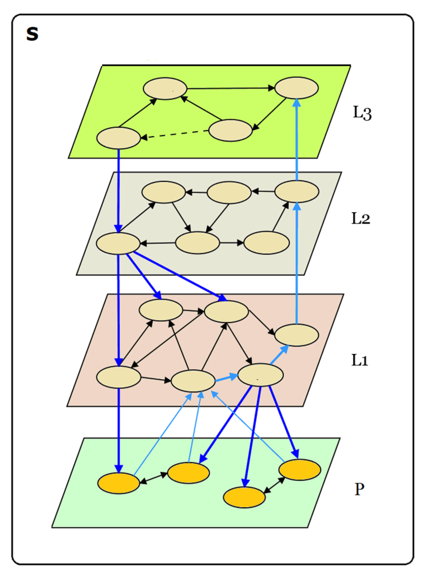
Figure 1 shows the architecture of a hierarchical control system S, where L₃ is the strategic control level, L₂ is the coordination level, L₁ is the executive level, and P is the level of production processes, elements, and subsystems (the control object). The flows of control and feedback signals are represented by arrows [23].

Next, we will consider the main stages of analyzing the state of system S and the snapshot generation methodology [24].

Step 1. We generate a graph G_T = (V_T, E_T), which is a model of the hierarchical level P. V_T is the set of vertices representing the nodes, subsystems, and business processes of this level, and E_T is the set of connections, such as information transmission channels.

Step 2. We determine the set of critical elements V_TR ⊂ V_T and the set of connections E_TR between V_TR elements—i.e., those elements whose failure could lead to the division of the system into several unrelated subsystems, thereby compromising the integrity of system S.

Step 3. We periodically analyze the state of V_TR and E_TR elements (based on snapshots over a given time period Δt).

Step 4. We generate graphs for levels L₁ and L₂. At the L₂ coordination level, for example, teams of performers are formed, and tasks are distributed within the team in an optimal manner, taking into account the status of team members (experience, qualifications, etc.). Assignment problems are solved—i.e., by assigning performers (machines) to perform tasks. For large systems, various optimization algorithms must be applied to solve assignment problems.

Let us now consider an example for system S, where it is necessary to manage the distribution of computing resources between hierarchy levels. We will choose the energy consumption level E as the generalized indicator of resource usage.

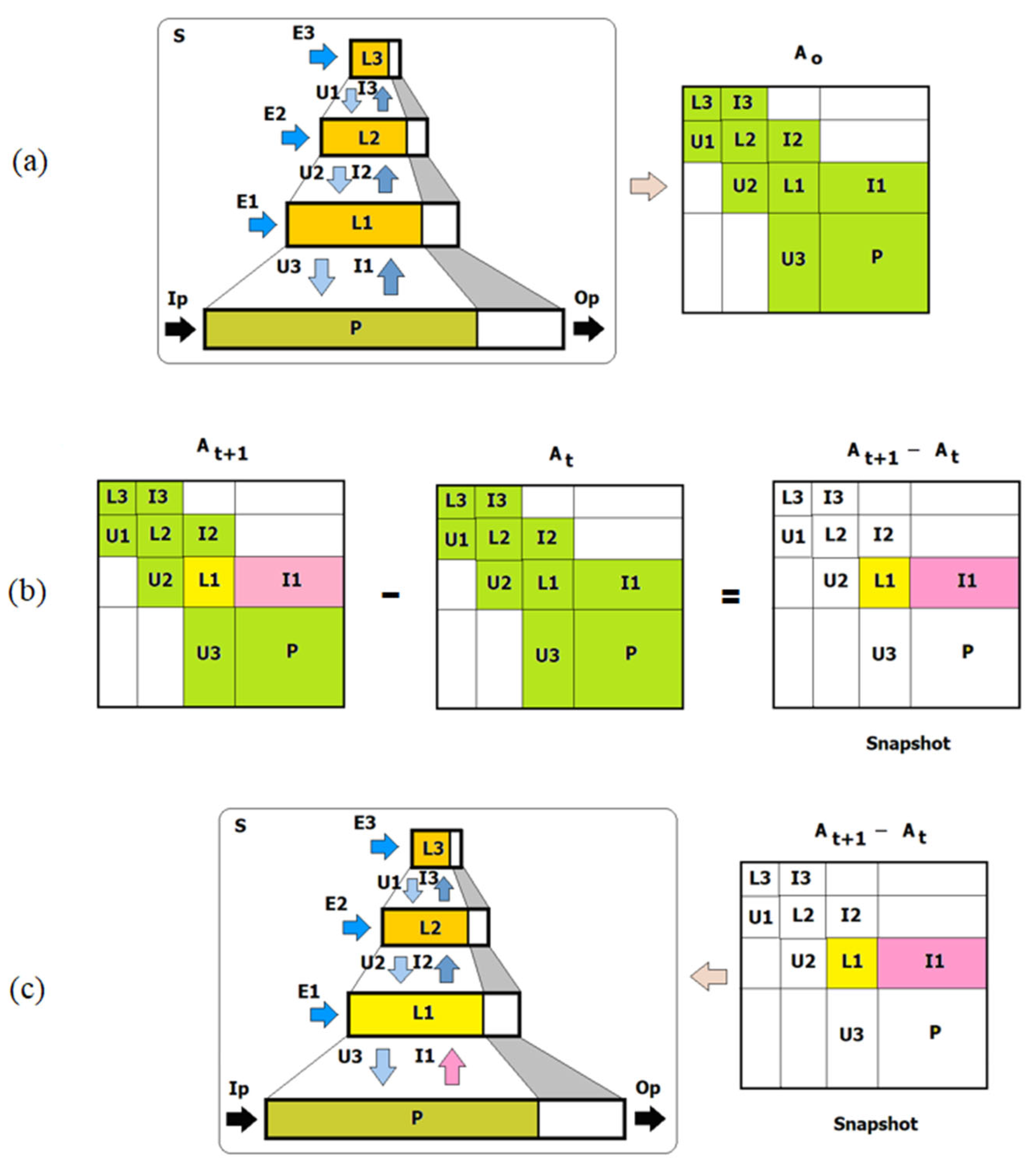
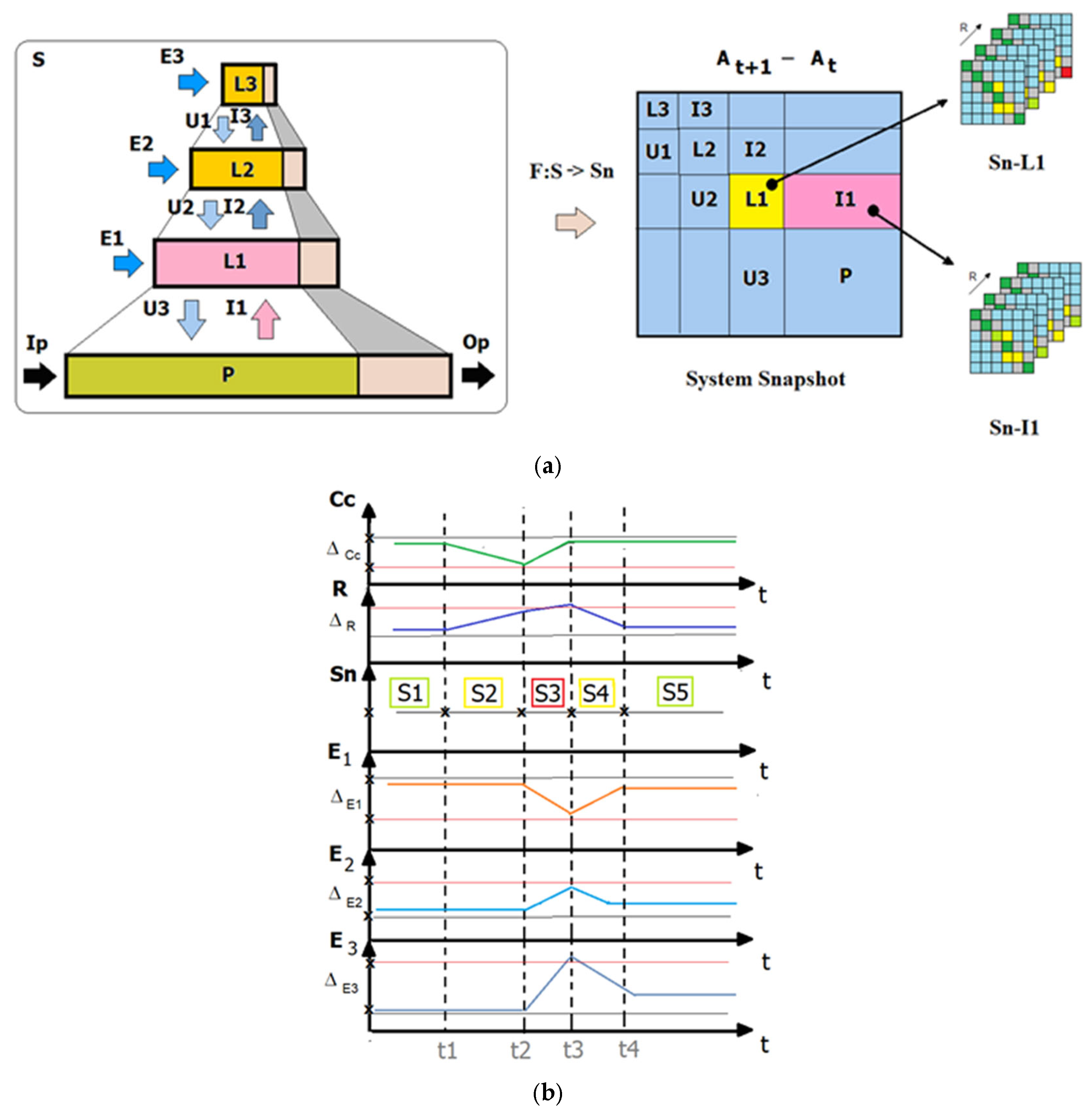
Figure 2 schematically represents a company’s hierarchical control system, where I_p is the input material flow; O_p is the output product flow; P is the enterprise (control object); E₁ is the electrical energy used to generate control command flows U₃ and feedback information flows I₁ by the executive level L₁; E₂ is the electrical energy used to generate control flows U₂ and information flows I₂ by the coordination level L₂; and E₃ is the electrical energy used to generate control flows U₁ and information flows I₃ by the strategic level L₃. In Figure 2, uncontrolled data flows are highlighted in gray and take into account interference, time delays, etc. Based on the obtained data, a basic snapshot of the system’s state in normal operation is generated, represented as a block matrix A₀ (see Figure 2a). The states of block matrix elements are highlighted according to color: green—normal state, yellow—potential failure state, and red—failure state. A snapshot is generated at times t + 1 and t (see Figure 2b). If the state of layer L₁ and data transmission channel I₁ changes, the system saves the changes and generates a snapshot (see Figure 2c).

Complex systems execute multiple business processes. Let us now consider the specifics of generating a snapshot of a business process’s state.

4. Creating a Business Process Snapshot

When creating business process snapshots, it is necessary to use business process description models that allow the system state to be assessed in terms of the quality of the business processes running in the system [25,26,27]. Models based on IDEF diagrams or BPMN diagrams can be used for this purpose. These models are developed by systems analysts who have up-to-date information on the structure and nomenclature of the company’s core business processes. The company’s information system (the enterprise’s ERP system) is then developed based on these approved (reference) models. BPMN diagrams are widely used to describe business processes, by which a sequence of processes, subprocesses, and activities is formed. 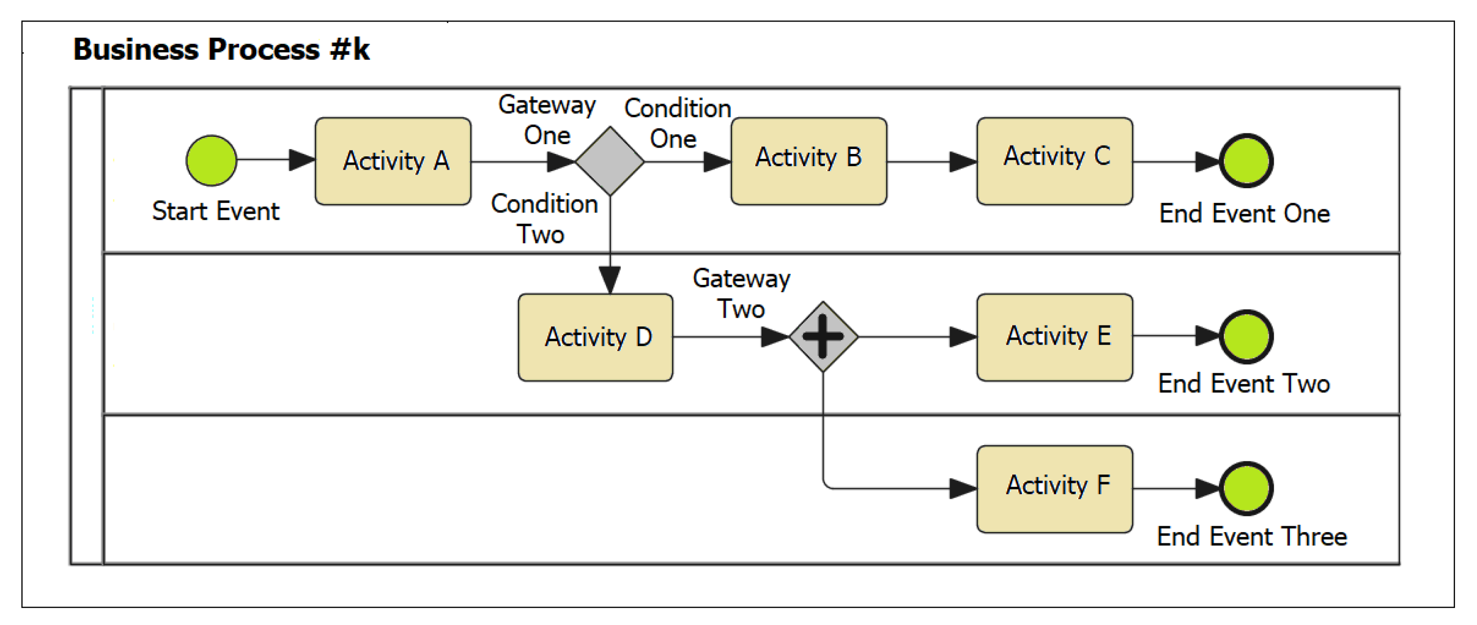Figure 3 shows an example of a BPMN diagram for business process #k. The business process includes six activities (A, B, C, D, E, F) and two decision-making blocks (Gateway One and Gateway Two). As a result of execution, business process #k can assume three states (End Event One, End Event Two, End Event Three).

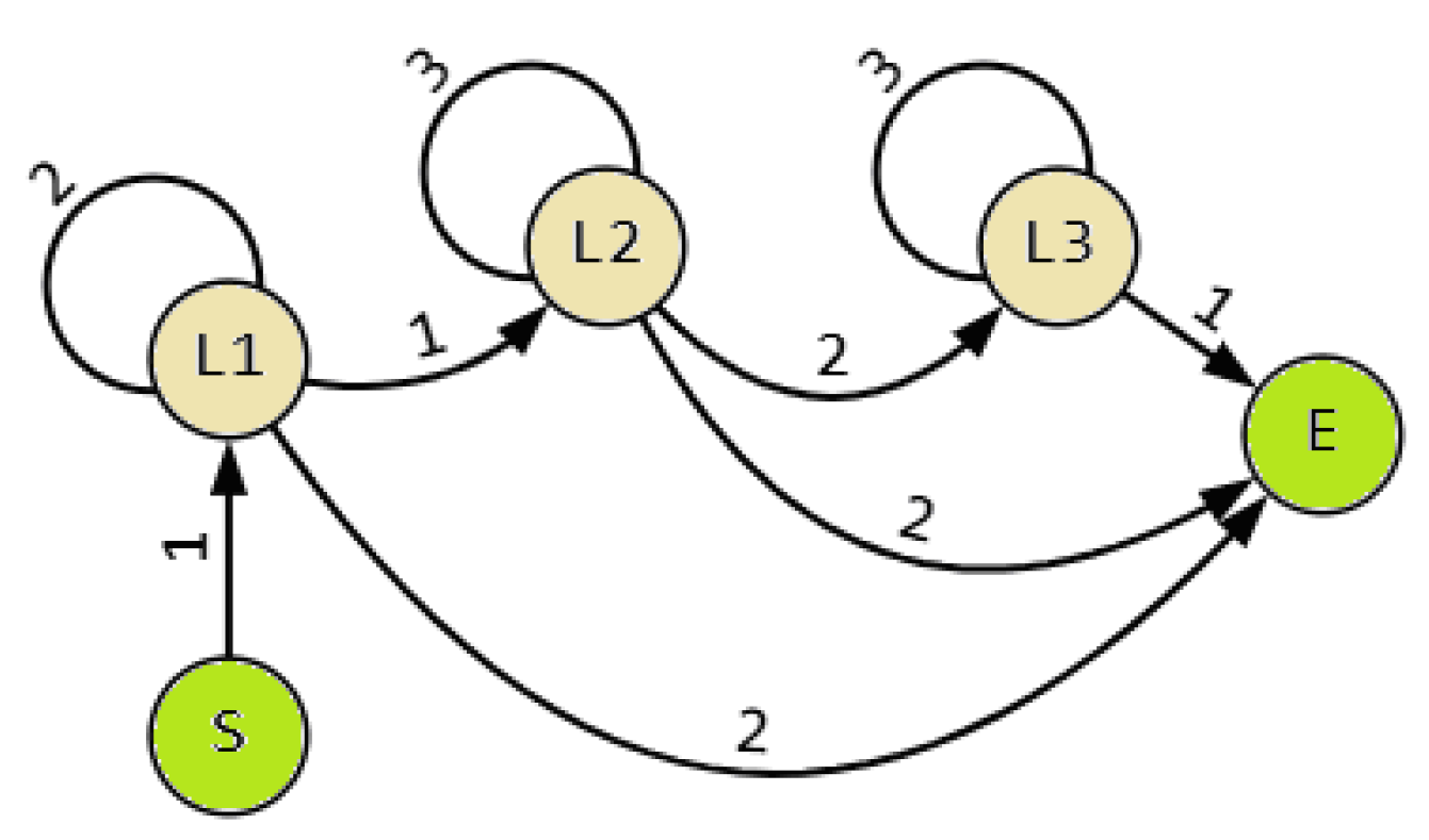
Based on this diagram, a software module for supporting this business process was designed, including implementation, interfaces, etc. Software implementations have been developed that allow for the analysis of the state of business processes based on this notation. The model shown in Figure 3 can be represented as a directed graph G (see Figure 4), where the following notation is used: node s—business process initialization; node l₁—activities A, B, and C; node l₂—activities D and E; node l₃—activity F; and node e—business process completion. The edge weights of the graph reflect the quantitative characteristics of the frequency of transitions from one node of graph G to another. This representation of the model allows the use of graph theory for analyzing the business process model.

A generalization of these two models is the DRAKON process description model. Let us now examine the details of using DRAKON for describing business processes and developing dynamic models, as well as the specifics of its use in generating snapshots of the system state S.

4.1. Building a Business Process Model Based on the DRAKON Language

Visual models based on business process description languages, such as IDEF, BPMN, and others, have become widely used to describe business processes in OTSs. When designing information systems within a process-based approach, these models are used to implement algorithms for supporting technological and organizational processes within a company.

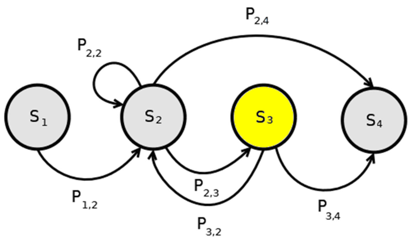
Various mathematical models, such as finite-state machine models, can be used to analyze discrete processes (business processes). Their construction requires statistical data sets reflecting the state of the machine and the probabilities of transitions from one state to another.

Figure 5 shows a finite-state machine model of a business process with four states:

M = (S, P),

(1)

where

S = (s_i, i = 1…4) is the set of business process states;

P = (p_ij, i = 1…4, j = 1…4) is the set of probabilities of transitions from one business process state to another.

If the ability to collect data on the model’s states and transitions from state to state at a given point in time is provided, the business process can be described as a finite-state machine.

DRAKON is a visual modeling language for dynamic processes that utilizes the concept of states and a tree-like structure for implementing computational processes. This is convenient for solving the problem of transitioning from describing business processes to representing them as a finite-state machine model [18,19,20].

The DRAKON language is particularly suitable for snapshot-based analysis because:

(i)

It explicitly represents process states as named icons, which directly correspond to the states of the finite-state machine model (1)–(2);

(ii)

Its rigid top-to-bottom and left-to-right flow rules reduce ambiguity when extracting the current state of a business process;

(iii)

The visual syntax is intuitive for domain experts, facilitating validation of the generated snapshots. These features make DRAKON preferable to generic BPMN when the primary goal is to monitor and capture discrete process states at defined time points.

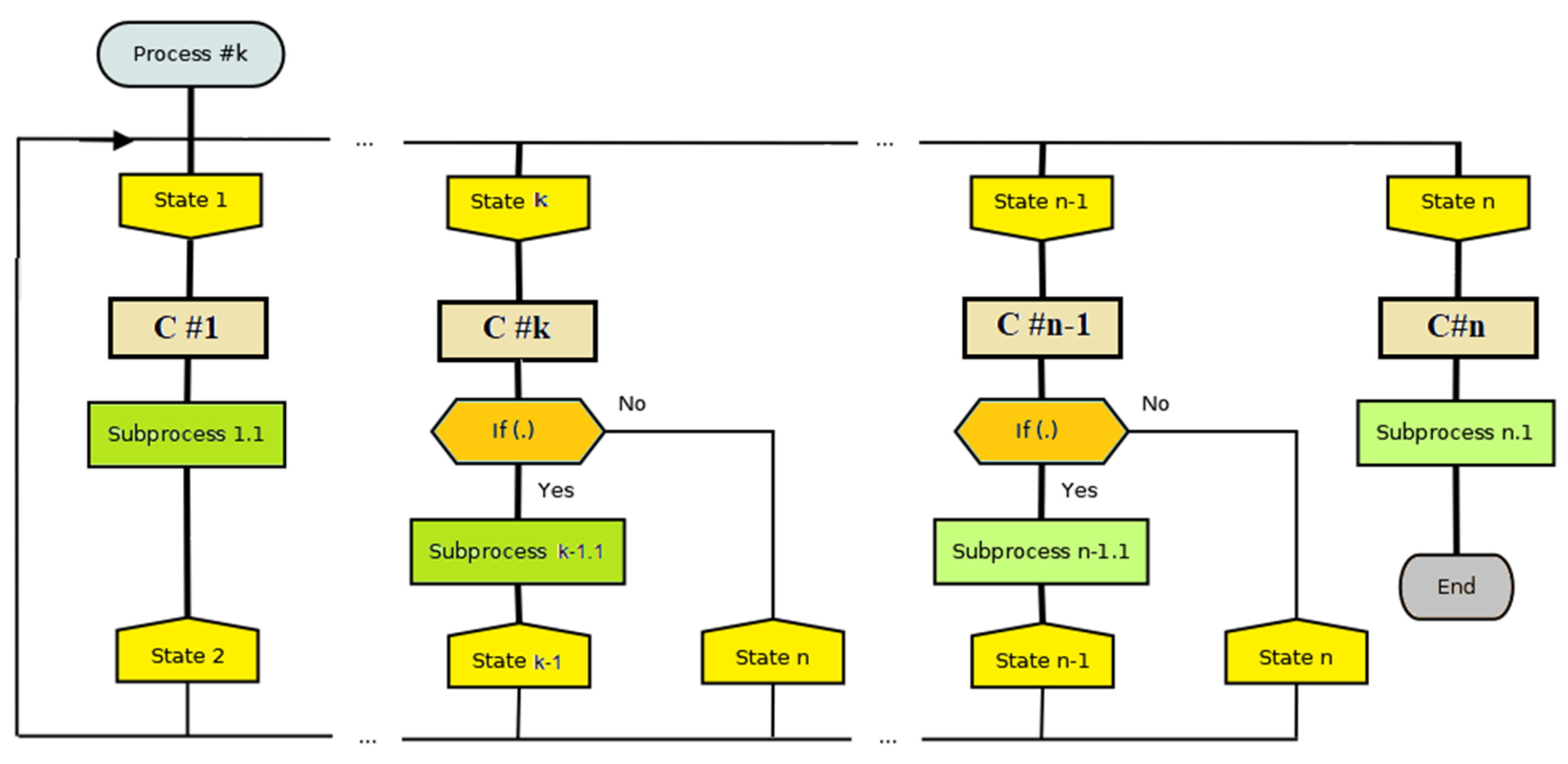
An algorithmic model describing the business process “Process #k” in the DRAKON language is shown in Figure 6. The states of the business process are represented by a set of states. When analyzing the execution logic of a subprocess, a transition is selected that transfers the business process to a new state:

M = (S, P, R, V, C)

(2)

where

S = (State #1, …, State #n−1, State #n) is the specified set of possible states of the business process “Process #k”;

P = (Subprocess #1.1, …, Subprocess #n−1.1, Subprocess #n.1) is the specified set of possible subprocesses;

R = ({if (.)}) is the set of transition conditions for selecting the next process or subprocess;

C = (C#i) is the set of memory blocks, in which i = 1 − n.

It should be noted that internal control flows are subject to the following rules. Internal control flows on the diagram branches progress from top to bottom, while for the outer loop, control flows from left to right. The business process execution algorithm itself includes several parts, represented by vertical branches. Each business process may include subprocesses, designated by the branch name at the top of the branch. The bottom of the algorithm execution branch contains the names of subsequent branches of possible transitions that are formed during the business process implementation. The DRAKON-based business process representation is intuitive for analysts and facilitates process analysis by managers when monitoring the modeling and implementation of algorithms in the information system, as well as during the algorithm verification process.

Next, we will consider the basic steps for creating a state snapshot.

4.2. Creating a Snapshot of a Distributed Business Process System

The time complexity of generating a snapshot of a large system is related to analyzing the state of multiple nodes and subsystems, and to collecting and processing data on their states. While we previously discussed the basic algorithms for generating a snapshot of an information system’s state, we note that these algorithms can be implemented in middleware or as functions of the core data processing algorithms within the ERP system itself [28]. When generating a snapshot of a business process, it is important to develop an automaton model with distinguishable states of the business process. Reliable protocols for transmitting data on the current state of the business process are required [29]. If necessary, the issue of visualizing business process states in a given state space of indicators can be addressed [30,31].

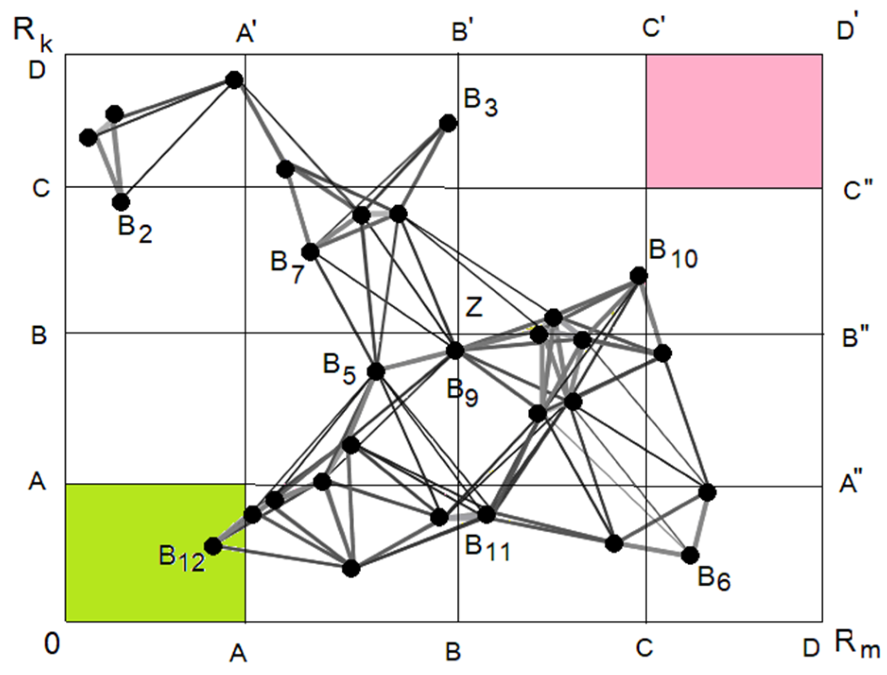
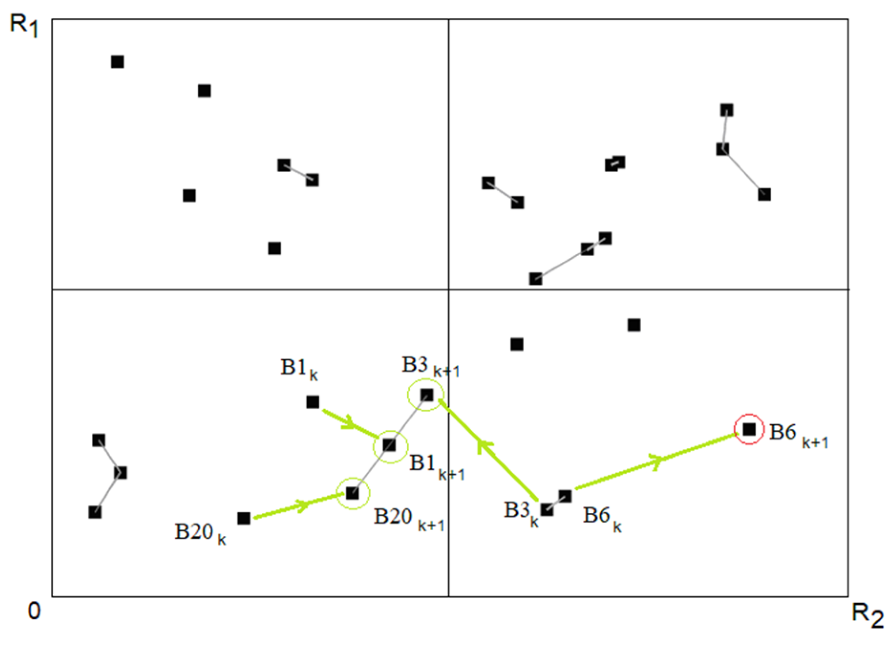
Figure 7 shows a generalized diagram of the state of a business process system as a stochastic graph, the vertices of which change their positions in a given metric state space:

G = (B_ij,V_ij), i = 1…n, j = 1…m,

(3)

where B_ij is a business process (graph vertex) in the space D(R_k,R_m); V_ij are the connections between processes (graph edges) that arise during interactions between business processes; and R_i is the i-th business process quality indicator.

We consider the algorithm for generating a graph snapshot.

• BPS (Business Process Snapshot) Algorithm:

Stage 1. We represent each business process as a finite-state machine using DRAKON diagrams. The set of states S_i and transition conditions C_i are formally recorded.

Stage 2. For each process, we define a metric vector (e.g., cycle time, waiting time, throughput, first-pass yield) and assign a state space.

Stage 3. We select a consistent data exchange protocol (e.g., marker-based Chandy–Lamport algorithm) to guarantee a globally consistent cut across all processes.

Stage 4. At the designated snapshot instant, we collect the current state of each process (the state label from the DRAKON diagram and the corresponding metric values). We then timestamp each record with the local node time.

Stage 5. We build a directed graph G = (B_ij,V_ij), where vertices B_ij correspond to business process instances positioned according to their metric vectors, and edges V_ij represent active interactions (e.g., message passing) at the snapshot moment.

Stage 6. We analyze the snapshot graph by identifying clusters of processes with similar states and detecting bottlenecks (e.g., vertices with high in-degree and long waiting times), which we then compare with previous snapshots to compute trend indicators.

Figure 8 shows an example of a snapshot of the business process’s system state at times t_k and t_k+1, generated based on the algorithm for generating a snapshot of the business process system state as presented above. The dynamic trajectories of the business processes at time t_k+1 form subgraphs—for example, G_s = (B_20k+1, B_1k+1, B_3k+1)—illustrating the joint state of the business processes in an arbitrary quadrant of the state space. When selecting control actions, the goal of control may be to ensure the system’s movement within a given business process’s state space.

4.3. The Problem of Analyzing the Quality of System-State Snapshots

The problem statement in the context of system S state snapshot analysis boils down to finding a balance between the accuracy (completeness) of the system-state assessment, reflecting the current system state and the cost of generating the snapshot. We choose the following as the objective function reflecting the accuracy of snapshot generation at time i:

$$∆\left(S_{real},S_{snap}\right)={\displaystyle \frac{1}{N}}{\displaystyle {\sum }_{i=1}^N}{\Vert {\mathbf{x}}_i^{real}-{\mathbf{x}}_i^{snap}\Vert }_2 ,$$

(4)

where $x_i^{real}$ and $x_i^{snap}$ are data structures reflecting the state of processes in system S at a given moment.

For the given problem, it is necessary to minimize function J over a given interval of a selected scale while respecting technological and budget constraints:

$$J={\displaystyle \frac{1}{K}}{\displaystyle {\sum }_{k=1}^K} {∆}_k\to \min .$$

(5)

We introduce constraints that take into account the accuracy of the estimate and the cost of generating a snapshot:

• Regarding snapshot generation frequency, the parameter q is determined by the process dynamics. If snapshots are generated without taking into account changes in the entropy of processes, this leads to a loss of information about intermediate stages of the process state. As the snapshot generation frequency increases, communication channels are overloaded, and the cost of generating an overall picture increases;
• Delays in synchronizing the processes of generating snapshots of the system state—i.e., the maximum allowable time difference between snapshot generation on different nodes (subsystems) of the system S;
• The cost of generating snapshots, reflecting the costs of storing and processing the data arrays required to generate snapshots, given the specified budget value C_max.

In distributed systems, when determining the optimal interval for generating a sequence of snapshots, the following are taken into account:

• The probability of detecting critical errors in processes P_f over a given time interval.
• The additional load on the computing nodes of the information system when an E_snap snapshot is generated.
• Snapshot frequency, where $∆t_{snap} \ge { \tau }_{min}$ (to prevent channel congestion).
• Synchronization of the maximum time difference data acquisition times between across system elements must be $\le {\delta }_{max}$.
• Cost is $C_{snap}\le C_{max}$, where $C_{snap}$ includes the costs of data collection, transmission, and storage.

It should be noted that when analyzing the state of a system S, it is necessary to develop a system-state monitoring protocol—i.e., determine which subsystems (nodes) to monitor, at what level of detail, and how often to take snapshots. This allows for the history of business processes to be reconstructed if necessary—i.e., it is necessary to ensure the ability to reconstruct the entire value chain based on a set of snapshots.

Distributed systems use metrics that reflect not only the pace of process execution but also the consistency of all subsystems within the distributed system. Let us consider the main metrics used for process analysis below.

Metrics based on process execution time (time-based metrics). These metrics typically include:

• Cycle Time. This is the time required to complete a process from start to finish. Snapshots allow one to determine on which node (subsystem or department) a process is stuck;
• Waiting Time (Idle Time). The portion of time a request or resource is idle between execution stages. In distributed systems, this is caused by information transfer delays or differences in execution rates;
• Throughput. The number of completed business processes per unit of time.

Quality-based metrics:

• First Pass Yield. The percentage of processes that pass through all system subsystems (nodes) without being returned for rework;
• Rework Rate. The frequency of business process reversion to the previous stage. Snapshots help identify “loops”—i.e., subsystems (nodes) that most often cause failures in distributed work.

Resource and technical metrics:

• Resource Utilization. Reflects the state of a subsystem—i.e., whether some subsystems (nodes) are overloaded while others are idle. Optimization here leads to balancing of the load between subsystems (nodes);
• Synchronization Gap. As an important metric for system snapshots, it reflects the difference between the actual time an event occurred and the time it was reflected in the overall system monitoring information system. For example, if we select a metric (e.g., Cycle Time) and use snapshot analysis to find critical paths in a process chain, then the solution to the optimization problem will involve changing the process parameters (redistributing resources, changing the transition logic) to improve the selected metric.

In large systems, there is an increase in energy consumption for processing large volumes of data, their transmission, and storage [32,33,34]. Let us now consider an illustrative example of solving the problem of redistributing energy between HCS levels in the event of an overload of information channels.

5. Example of a Solution for Optimizing Energy Consumption in HCSs

Let us consider an example of decision-making based on analyzing snapshots of the company’s status. Control signals and decisions are transmitted via communication channels, and information about the results of control actions is transmitted to higher control levels. For simplicity, time and energy consumption are measured in conventional units.

The control system includes three control levels (L₁–L₃) and a production level P (Figure 9a). In normal operation, the energy consumption of each level is: E₁ = 5, E₂ = 3, and E₃ = 2 (conventional units). The total baseline energy consumption is 10 units, so the global constraint is total power E₁ + E₂ + E₃ ≤ 10.

Each control level has a local MPC controller that minimizes a quadratic cost function over a prediction horizon of h = 5 steps (Figure 9b), subject to local and global constraints. The levels’ controllers exchange predicted control trajectories and iteratively agree on a feasible energy consumption allocation.

At time t₂, a critical situation arises at the production level P, causing an overload of the feedback channel I₁. The required data transmission rate increases, and the executive level L₁ must raise its polling frequency. If no action is taken, E₁ would rise to 8 units, pushing total consumption beyond the maximum allowable limit E_max = 11 units, risking overheating and reliability problems. A snapshot taken over the time period t₁–t₄ (Figure 9b) reveals the overload of I₁ (state red) and the resulting delay at L₁ (state yellow). The risk curve R(t) is estimated from the snapshot data. To keep the total energy within the limit, a distributed model predictive control (DMPC) scheme is applied.

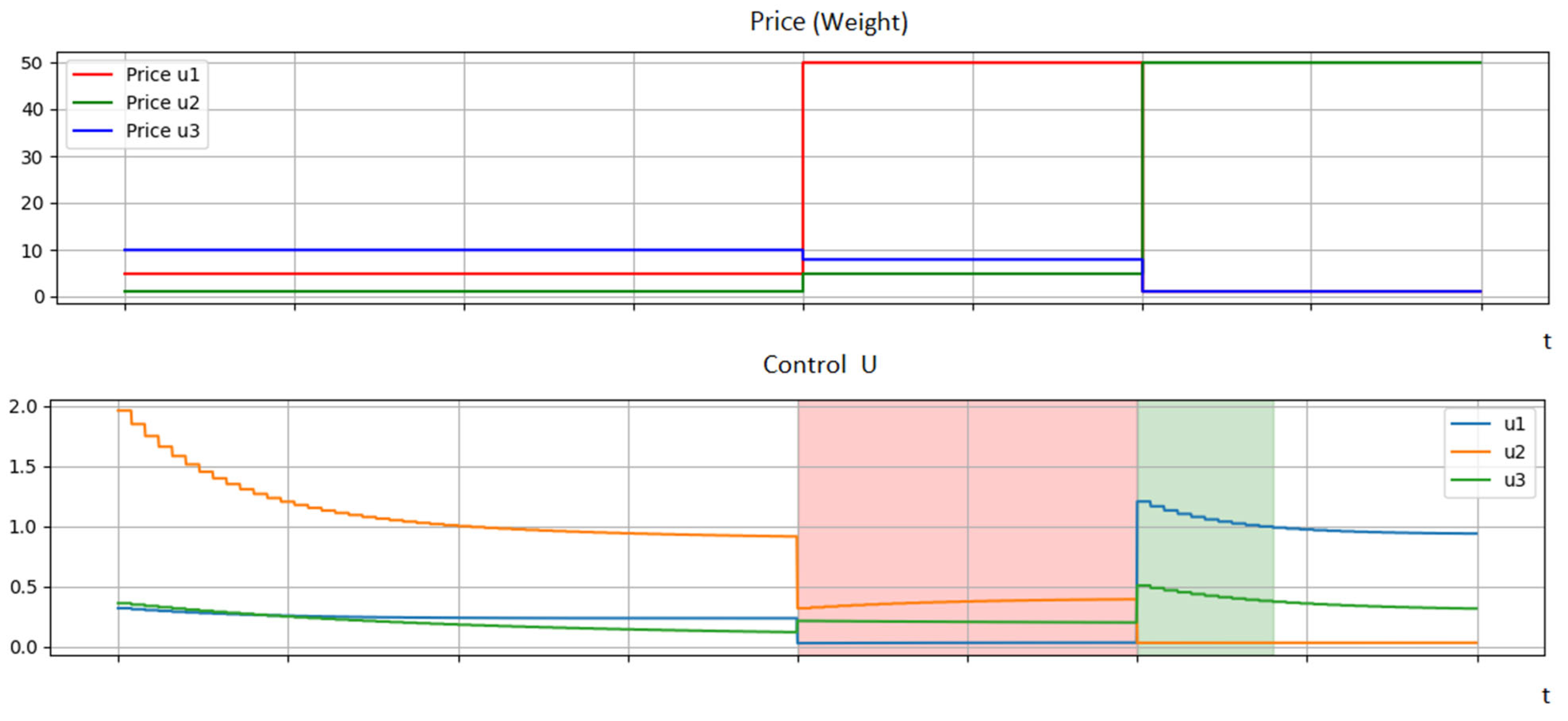
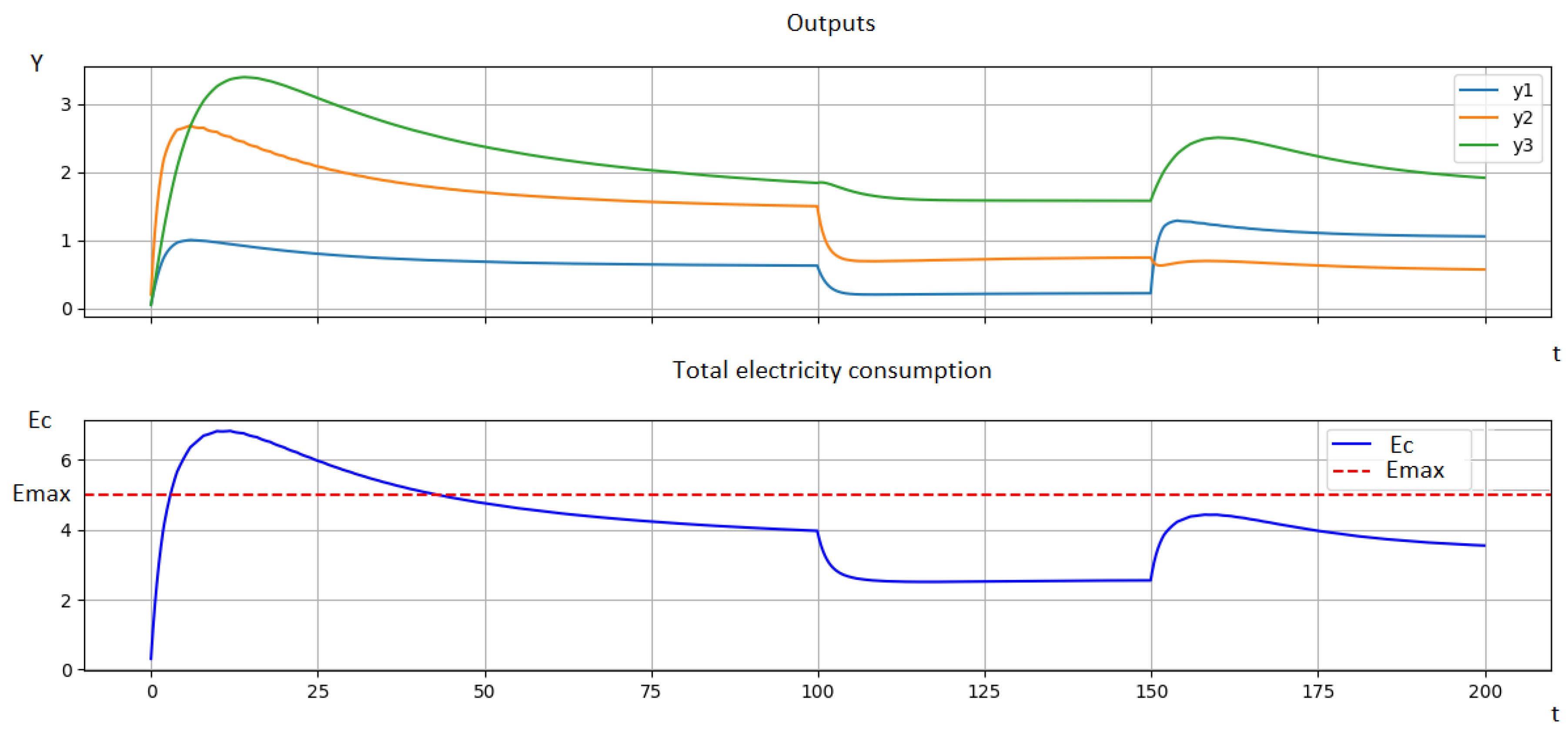
Figure 10 shows the results of modeling the response of the HCS energy consumption management system at various levels, which helps maintain the overall HCS energy consumption level.

Figure 11 displays the resulting energy consumption per level and the total consumption, demonstrating that the DMPC strategy successfully maintains the total consumption below E_max while preserving the most critical control function at L₁. The example, though illustrative, shows how snapshot-derived state information enables real-time energy redistribution in a hierarchical system.

It should be noted that redistributing power consumption between levels may temporarily reduce the system’s functionality, which helps ensure system survivability during the critical response phase. After the system has been restored, power consumption at the control levels is restored.

6. Conclusions

This paper has examined the problem of analyzing the state of large-scale organizational–technical systems controlled by hierarchical distributed systems. It has been shown that the execution of numerous parallel technological and business processes, which require synchronization and considerable energy expenditure, necessitating the formation of an up-to-date picture of the system’s state at all control levels.

The concept of a snapshot of the organizational–technical system’s state has been introduced, enabling system assessment within the framework of selected process performance criteria and supporting well-founded decisions at all hierarchy levels. Procedures for constructing snapshots have been analyzed, including copy-on-write, the Chandy–Lamport algorithm, cloud orchestration, and log-based point-in-time recovery.

DRAKON has been proposed as a design language, distinguished by its clarity in representing states and transitions, which simplifies business process modeling alongside BPMN notations and finite-state machines. An optimization problem has been formulated to minimize the deviation between the snapshot state and the real system state under constraints on snapshot frequency, synchronization delay, and cost.

A numerical example has demonstrated that distributed model predictive control (DMPC) enables energy redistribution among the levels of a hierarchical control system based on the analysis of the acquired snapshot. The results demonstrate the potential application of the proposed methodology for improving energy efficiency and control quality in large-scale organizational and technical systems.

It should be noted that implementing the proposed methodology will require the development of middleware. In some cases, situational management methods will need to be used, which will require additional research. Further research is expected to consider the metrics discussed to ensure the quality of snapshots.