Article

CTA-Net: A Cross-Temporal Attention Network for Change Detection in Remote Sensing Imagery

1
Institute of Automation and Information Technologies, Satbayev University (KazNRTU), Almaty 050013, Kazakhstan
2
School of Software Engineering, Astana IT University, Astana 010000, Kazakhstan
3
Institute for Computational and Data Sciences, The Pennsylvania State University, University Park, PA 16802, USA
4
Office of Registrar, Kazakh National Medical University Named After S.D. Asfendiyarov, Almaty 050012, Kazakhstan
*
Authors to whom correspondence should be addressed.
Big Data Cogn. Comput. 2026, 10(7), 225; https://doi.org/10.3390/bdcc10070225
Submission received: 21 May 2026 / Revised: 27 June 2026 / Accepted: 30 June 2026 / Published: 6 July 2026
(This article belongs to the Section Artificial Intelligence and Multi-Agent Systems)

Abstract

Accurate change detection in high-resolution remote sensing imagery is essential for urban planning, land-use monitoring, and disaster response. This study introduces CTA-Net, a Cross-Temporal Attention Network for binary change detection in bi-temporal optical imagery, designed to improve robustness against pseudo-changes caused by illumination variation, seasonal effects, and sensor noise. The proposed method employs a shared Siamese encoder with multi-scale Cross-Temporal Attention modules that derive spatial and channel attention from L2 feature differences, along with a lightweight confidence estimation head for per-pixel uncertainty modelling. A hybrid loss function combining confidence-weighted binary cross-entropy and focal loss is used to address class imbalance. Experiments on the LEVIR-CD dataset demonstrate that CTA-Net achieves an overall accuracy of 98.99%, an F1-score of 87.68%, an Intersection over Union of 78.06%, a Cohen’s kappa of 0.8715, and a Matthews Correlation Coefficient of 0.8721, with stable convergence and minimal overfitting. Qualitative and calibration analyses further indicate that the model produces interpretable attention maps and reliable probabilistic outputs. To evaluate cross-domain generalization, we conduct a transfer learning case study on multispectral Sentinel-2 agricultural imagery. The model is adapted to 11-channel input and fine-tuned on automatically generated change masks derived from NDVI-delta thresholding. Under this supervision protocol, CTA-Net achieves an F1-score of 95.18% and an IoU of 90.81% on a held-out test region, with balanced precision and recall. While these results demonstrate effective adaptation across sensor modality, spatial resolution, and semantic domain, the evaluation reflects agreement with the mask generation procedure rather than independently annotated ground truth. While CTA-Net shows strong performance and reasonable interpretability, its cross-domain evaluation is limited by the use of automatically generated labels. As a result, the reported transferability should be interpreted cautiously until validated on human-annotated datasets.

1. Introduction

Land-cover change mapping using multi-temporal satellite and aerial imagery is a fundamental task in Earth observation that has many applications, including monitoring urban expansion, disaster assessment, tracking deforestation and managing infrastructure [1,2,3,4,5,6]. With the expanding availability of very-high-resolution optical sensors (VHR) and large geospatial archives, there is a growing need to develop accurate, scalable and automated change detection techniques [7,8,9].
Several traditional change detection methods have been extensively studied such as image differencing [10], change vector analysis [11] and post-classification comparison [12]. But they are subject to degradation of performance caused by the effects of the atmosphere, changes in illumination, the changes in season and the geometric misregistration [13]. The fully convolutional networks (FCNs) [14,15], encoder–decoder architectures [16] and Siamese networks have significantly enhanced robustness by learning hierarchical feature representations from the image data directly. Even with all these developments there are still three significant challenges. To begin with, there is a class imbalance in benchmark datasets like LEVIR-CD, where changed pixels make up only a small fraction of the total (less than 5%). This causes a biassed optimization and low recall from the datasets [17,18,19]. Second, some light variation, seasonal changes and inconsistencies in the sensors can lead to pseudo-changes, which can result in false detections [20,21]. Thirdly, many existing techniques do not explicitly indicate the spatial areas and feature channels that are most important in capturing meaningful temporal differences, which can result in the inability to distinguish relevant differences from irrelevant changes [22,23,24].
To overcome these problems, many Siamese-network-based architecture have been proposed [25,26,27]. Shared-weight encoders are used to obtain temporally consistent feature representations; the temporal information is typically represented using feature subtraction, concatenation or correlation [28,29]. Moreover, multi-scale feature fusion and deep supervision are used to enhance the fusion of high-level semantic information and local spatial information [30,31]. However, in general, these strategies are based on fairly straightforward approaches to feature fusion that do not make the most of the discriminative nature of temporal differences, especially when pseudo-changes are present [20,21,29].
Attention mechanisms have recently become an effective means of improving feature representation in deep neural networks [32,33,34,35]. Transformer-based self-attention models are proven to have an impressive performance in remote sensing change detection [22,35,36] due to their ability to retain the long-range spatial and temporal dependencies. Similarly, CNN attention modules like CBAM [32] and SE-Net [34] boost feature representations by focusing on informative spatial regions and channels. The methods, however, typically calculate the attention from individual feature maps or a combination of fused bi-temporal representations, which means they have to infer the discrepancies in time implicitly. An indirect formulation can decrease the discriminative signal in difficult imaging situations such as changes in illumination or seasonal changes. Furthermore, uncertainty estimation and prediction calibration are still relatively underexplored fields of importance for disaster response and other safety-critical applications [37].
Considering these drawbacks, this work presents a difference-guided attention mechanism, which infuses spatial and channel attention directly based on the L2-norm of temporal feature differences, instead of single or combined feature representations. The proposed design is designed to enhance the discrimination of real change from pseudo-changes while being efficient in terms of computation, with a light convolutional implementation.
In this paper, we propose the Cross-Temporal Attention Network (CTA-Net) for robust bi-temporal change detection. The main contributions are as follows:
  • We develop a shared Siamese encoder with four hierarchical feature extraction stages to produce temporally consistent feature representations.
  • We introduce multi-scale Cross-Temporal Attention (CTA) modules that generate both spatial attention and channel recalibration directly from L2-based temporal feature differences, enabling the network to emphasize semantically meaningful changes.
  • We incorporate a lightweight per-pixel confidence estimation head that models predictive uncertainty and enables confidence-aware supervision during training.
  • We propose a hybrid loss function combining confidence-weighted focal loss with standard focal binary cross-entropy to improve optimization under severe class imbalance and noisy observations.
  • We perform a comprehensive evaluation on the LEVIR-CD benchmark using ROC and precision–recall analysis, confusion matrices, Cohen’s kappa, Matthews Correlation Coefficient, calibration curves, and qualitative visualization of learned attention maps to demonstrate the effectiveness and interpretability of the proposed method.

2. Related Work

2.1. Traditional Change Detection

The traditional methods used for studying change detection in remote sensing were mainly based on direct algebraic processing of pixel level radiometric data [12]. Image differencing and image rationing are some of the techniques used to produce change magnitude maps by computing the difference or ratio between bi-temporal images at the pixel level [10]. These are very efficient for computational purposes, but suffer from high sensitivity to noise, lighting conditions and atmospheric effects [1].
To overcome some of the above limitations the change vector analysis (CVA) [11] was proposed that represents temporal change as vectors in multispectral feature space, thus capturing both the magnitude and direction of change. This provides a more expressive representation of the spectral variation, but the choice of threshold value and sensitivity to radiometric inconsistencies are still important considerations [2].
A more abstract approach was presented by post-classification comparison [12], which classified each temporal image independently and compared the thematic maps obtained from each classification. This method helps to minimize spectral inconsistencies between acquisition times but has error accumulation since errors in each classification add up in the final change map [13].
The traditional methods rely on strong assumptions about the data consistency, manual thresholding and handcrafted features [18]. As a result, their performance is greatly affected in real-world scenarios of misregistration, seasonal variation and sensor noise.

2.2. Deep Learning-Based Change Detection

With the advent of deep learning [14,38,39], remote sensing change detection has become one of the most important applications of deep learning in Earth observation because it enables feature representations to be learned directly from raw imagery [19]. Fully convolutional networks (FCNs) have emerged as a standard framework for dense prediction tasks [15].
A seminal contribution to deep learning-based change detection was made by Daudt et al. [9], who introduced Siamese fully convolutional network architectures (FC-EF, FC-Siam-conc, and FC-Siam-diff). These architectures process images acquired at different times using shared encoder weights to ensure temporal feature consistency. Their work demonstrated that explicitly modelling temporal differences within a deep learning framework can substantially improve performance compared with traditional change detection approaches.
Building upon these early Siamese architectures, numerous CNN-based encoder–decoder networks have been developed to improve feature representation and temporal interaction. SNUNet [25] employs densely connected Siamese encoder–decoder pathways to enhance feature reuse and gradient propagation, while ensemble channel attention further improves discriminative capability. More recently, transformer-based architectures have attracted considerable attention because of their ability to model long-range dependencies and global contextual relationships. BIT [22] incorporates transformer modules into a ResNet-based framework to capture global temporal interactions, while ChangeFormer [36] employs a hierarchical transformer encoder and dedicated difference modules to strengthen feature interaction across time. These approaches have achieved strong performance in change detection, although they typically require greater computational resources than lightweight CNN-based alternatives.

2.3. Attention Mechanisms in Remote Sensing

In recent years attention mechanism has attracted much attention in remote sensing [40] and has shown good performance in the fields of object detection, scene classification and semantic segmentation [41]. Attention modules dynamically reweight feature responses to focus neural networks on informative spatial regions and feature channels and suppress less relevant information.
Channel attention mechanisms like Squeeze-and-Excitation (SE) block [34] explicitly learn inter-channel dependencies for adaptively re-calibrating channel responses. Spatial attention mechanisms, such as Convolutional Block Attention Module (CBAM) [32] add to this process by identifying salient spatial locations in feature maps.
Attention mechanisms have been shown to be effective in remote sensing change detection to identify true structural changes from pseudo-changes due to variation in illumination, seasonal variations, or sensor noise. Most of the current methods, however, calculate attention based on the individual temporal feature maps or the combined bi-temporal attention representation, which forces the network to learn temporal inconsistencies latent in the data. Consequently, temporal feature differences that are explicit and carry discriminative information might not be fully utilized [21].
Recent work has started to investigate attention mechanisms based on temporal difference features to focus on salient differences and to attenuate irrelevant variations. While these methods have shown promise in making attention more robust, additional studies are required to create attention mechanisms that explicitly incorporate temporal differences across multiple feature scales in a computationally efficient manner.

2.4. Loss Functions for Imbalanced Segmentation

One of the most significant issues in a binary change detection problem is the great imbalance between unchanged and changed pixels [1]. In many datasets, like LEVIR-CD, the number of unchanged pixels can be greater than the number of changed pixels by more than 20:1, which cannot be learned by traditional loss functions.
Although popular, binary cross-entropy (BCE) loss is biassed towards the majority class and may lead to low recall for the minority (changed) class. Focal loss [42] solves this by assigning less importance to easy samples, which are likely to be well classified, and giving more weight to difficult samples, which are less likely to be well classified.
Region based losses like Dice loss [43] and Intersection over Union (IoU) loss directly optimize overlap based evaluation metrics and are therefore very suitable for imbalanced class segmentation. But these losses could be unstable in the early period of training or if predictions are highly uncertain.
Confidence-aware learning strategies have been developed to further boost robustness. We approximate the per-pixel loss with a confidence-weighted formulation, which multiplies the losses with the per-pixel uncertainty predictions. This mechanism helps to lessen the effect of high-confidence wrong predictions and buffer against noisy or ambiguous samples. This hybrid objective, coupled with focal loss, allows more stable optimization and better generalization in more difficult real-world cases.
Although there have been significant advancements in recent change detection techniques based on deep learning, there are still some limitations. Current methods mostly use a fusion of features or attention mechanisms on concatenated or individual temporal features, that do not fully utilize the discriminative structure of explicit temporal differences. Furthermore, although attention modules have achieved robustness to pseudo-changes, there are not many that explicitly include uncertainty estimation, which can lead to predictions with noise in extreme cases like during variation in illumination or seasons. In addition to that, the class imbalance problem is solved by common loss reweighting approaches without considering the confidence-aware learning that considers the reliability of prediction. It is worth noting that this limitation is architectural rather than purely computational: even transformer-based methods with sufficient capacity to model long-range dependencies [22,36] generally compute attention from fused or individually encoded temporal representations rather than from an explicit difference signal and therefore do not guarantee that attention is anchored to quantified temporal change. Thus, a unified solution that (i) explicitly models discrepancies between features across time, (ii) utilizes attention mechanisms, guided by such discrepancies, across multiple scales, and (iii) integrates uncertainty estimation into the optimization process is still needed. To overcome these limitations, the proposed CTA-Net extends the domain-specific attention mechanism by Cross-Temporal Attention, which is based on feature difference, while simultaneously incorporating a confidence-aware learning approach that enhances the robustness and interpretability of the approach and performance in real-world change detection applications.

3. Materials and Methods

This section describes the LEVIR-CD dataset, preprocessing pipeline, proposed CTA-Net architecture, loss function, and training procedure used for the experimental evaluation.

3.1. LEVIR-CD Dataset

The LEVIR-CD dataset [40] is a popular benchmark for developing change detection in VHR remote sensing images. It consists of 637 pairs of 1024 × 1024 -pixel RGB images captured by Google Earth over 20 regions covering Texas, USA, at a ground sampling distance of ∼0.5 m. The gap between image pair(s) is 5 to 14 years. Newly built and demolition of buildings are delineated in change annotations as binary masks. There are 445 pairs in the training set, 64 pairs in the validation set and 128 pairs in the test set.
Table 1 reveals that the changed-pixel class only makes up about 4.2 % of all pixels, which is an extreme level of class imbalance. This distribution requires the use of focal-based loss functions and calls for the use of more than just accuracy in the assessment, including recall-sensitive metrics like F1, IoU, and Kappa.

3.2. Preprocessing

All images are RGB (three-channel) and the raw DN values are normalized to range [0, 1] by pixel value/255. No histogram matching and atmospheric correction is done, so that the proposed attention mechanism can be trained to be robust to inter-image radiometric variations. Each image pair consists of two RGB images with a resolution of 1024 × 1024 pixels. The pair is fed directly into the same Siamese encoder.
During training, no data augmentation is used, such as random flipping, rotation, or colour jittering. This design separates the performance improvement of the proposed CTA modules, confidence-aware learning strategy and loss formulation from that of the augmentation to give a proper evaluation of the proposed architecture with minimal preprocessing. In recent change detection studies, data augmentation has proven to be effective to make the system more robust, especially for small or low-contrast changes, but testing the augmentation strategies is left for future work.

3.3. DataLoader Configuration

In training, the image pairs are sampled so that the order of the mini-batches is random with PyTorch 2.6 DataLoader, while in the validation and testing stages, the order of the mini-batches is a fixed sequence. The workers were set to zero for compatibility with the GPU environment. The test set comprises 128 image pairs, resulting in a total of 67,108,864 pixels being assessed of which 4.2% (2,816,268) are classified as ‘change’.

3.4. Proposed Network Architecture

While the spatial attention component is inspired by CBAM [32] and the channel attention follows SE-network principles [34], the novelty of the CTA module lies in deriving both attention maps directly from L2-norm temporal feature differences rather than from individual or fused feature representations, enabling change-driven feature refinement at multiple encoder scales. Overall CTA-Net architecture is shown in Figure 1. The network takes as input a pair of bi-temporal images ( I A , I B ) R H × W × 3 and outputs a per-pixel change probability map y ^ [ 0 ,   1 ] H × W and a per-pixel confidence map c [ 0 ,   1 ] H × W . The architecture comprises four parts: (i) a shared Siamese Encoder, (ii) multi-scale Cross-Temporal Attention modules, (iii) an asymmetric decoder with skip connections, and (iv) dual output heads for change prediction and confidence estimation.
The encoder processes all temporal images having the same set of weights, and thus the representations of the features over time are comparable. It comprises three convolution blocks, each of which contains a max pooling layer, which are interleaved, followed by a bottleneck block:
e n c 1 : C o n v ( 3 32 ,   3 × 3 ) B N R e L U   M a x P o o l ( 2 × 2 )
e n c 2 : C o n v ( 32 64 ,   3 × 3 ) B N R e L U   M a x P o o l ( 2 × 2 )
e n c 3 : C o n v ( 64 128 ,   3 × 3 ) B N R e L U   M a x P o o l ( 2 × 2 )
b o t t l e n e c k : C o n v ( 128 256 ,   3 × 3 ) B N R e L U
where:
  • C o n v ( C i n C o u t , K ) denotes a convolution layer with:
    C i n : number of input channels.
    C o u t : number of output channels.
    K : kernel size.
  • B N denotes batch normalization.
  • R E L U denotes the Rectified Linear Unit activation.
  • M a x P o o l ( 2 × 2 ) denotes max pooling with ( 2 × 2 ) window.
For an input image of 1024 × 1024 pixels, the encoder produces feature maps at spatial resolutions of 1024 × 1024 (level 1, C = 32 ), 512 × 512 (level 2, C = 64 ), 256 × 256 (level 3, C = 128 ), and 128 × 128 (bottleneck, C = 256 ). CTA-Net is lightweight and has a total number of trainable parameters of about 1.2 M, making it ideal for deployment in resource-limited environments.
To justify this design choice, we trained three additional model variants with different capacities: CTA-Net-S (0.6 M parameters, F1 = 84.31%), the proposed CTA-Net (1.2 M, F1 = 87.68%), CTA-Net-L (2.8 M, F1 = 88.12%), and CTA-Net-XL (5.1 M, F1 = 88.37%). This marginal increase in the F1-score between 1.2 M and 5.1 M parameters is just a 0.69 percentage point, and the computational cost is over 4 × higher. Thus, the 1.2 M configuration is the best compromise between the detection performance and the computational cost.
The CTA module is computed at every scale and works on a temporal feature tensor F R B × T × C × H × W with T = 2 . It goes on like this:
Step 1—Temporal Difference Magnitude: Calculate the L2-norm of the per-pixel temporal difference δ = | | F 1 F 2 | | 2 , norm taken along the channel dimension, δ R B × 1 × H × W .
Step 2—Spatial Attention: Pass a single 3 × 3 convolutional layer and sigmoid activation function through δ to give a spatial gate A s [ 0 ,   1 ] B × 1 × H × W . This gate is used for highlighting the pixels where the temporal feature difference is spatially consistent.
Step 3—Attended Feature: F ^ = F 1 A s , with being element-wise multiplication, broadcasted along the channel dimension. This is used to modulate the pre-change feature using the change saliency map.
Step 4—Channel Attention (SE-style): Compute a global average-pooled descriptor from F ^ , pass it through two 1 × 1 convolutions with reduction ratio r = 8 , and apply sigmoid to obtain A c [ 0 ,   1 ] B × C × 1 × 1 . The final product is F ^ A c .
The CTA module operations are formally defined as follows. Temporal feature maps F 1 ,   F 2 R B × C × H × W are given as:
δ = | | F 1 F 2 | | 2 R B × 1 × H × W
A s = σ ( C o n v 3 × 3 ( δ ) ) 0 ,   1 B × 1 × H × W
F = F 1 A s R B × C × H × W
A c = σ ( W 2 R e L U W 1 G A P F ) 0 ,   1 B × c × 1 × 1
F = F A c R B × C × H × W
where:
  • F 1 , F 2 denote temporal feature maps at the same encoder scale.
  • B , C , H , W denote batch size, number of channels, height, and width respectively.
  • δ denotes the L2-norm temporal difference magnitude.
  • A s denotes the spatial attention gate.
  • F denotes the spatially attended feature map.
  • A c denotes the channel attention vector.
  • F denotes the final attended output *.
  • denotes element-wise multiplication.
  • σ denotes sigmoid activation.
  • G A P denotes global average pooling.
  • W 1 R C r × C , W 2 R C × C r are learnable projection matrices with reduction ratio r = 8.
It is worth clarifying the choice of the L2-norm magnitude δ , rather than the signed pixel-wise difference F 1 F 2 , as the input to the spatial attention gate. Pixel-wise subtraction is computationally cheaper and preserves signed, per-channel directional information, whereas δ compresses this information into a single non-negative magnitude value. This is an intentional simplification: the spatial gate A s is designed to answer a magnitude question (how much change occurred at a given location), not a directional one, and a non-negative, rotation-invariant signal is naturally suited to this role. Critically, directional information is not discarded from the network’s main representational pathway—the spatially gated feature F in Equation (7) retains the full signed multi-channel representation of F1, and the channel attention A c in Equation (8) is computed from this full-channel representation rather than from δ . The loss of directional information is therefore confined to the gate-generation branch and does not propagate into the main feature pathway.
This lightweight formulation has a linear complexity while retaining spatially and spectrally localized change information.
The decoder is the inverse of the encoder, using three transposed convolutional upsampling layers. The upsampled bottleneck representation is added to the attention-gated encoder feature map at the same scale for each stage:
d 3 = u p ( e 4 a t t ) e 3 a t t C o n v B l o c k ( 256 ,   128 )
d 2 = u p ( e 3 a t t ) e 2 a t t C o n v B l o c k ( 128 ,   64 )
d 1 = u p ( e 2 a t t ) e 1 a t t C o n v B l o c k ( 64 ,   32 )
where:
  • u p denotes bilinear upsampling by a factor of 2.
  • denotes element-wise addition.
  • e 1 a t t ,   e 2 a t t , e 3 a t t , e 4 a t t denote attention-gated encoder features at scales 1–4.
  • d 1 ,   d 2 , d 3 denote decoder feature maps at corresponding scales.
  • C o n v B l o c k ( C i n ,   C o u t ) denotes a convolutional block with C i n input channels and C o u t output channels.
Fine spatial details in the early layers of the encoder are important, e.g., for proper delineation of building boundaries with 0.5 m resolution and are preserved in skip connections.
To decrease the number of decoders to 16 channels, a two-stage convolutional head is implemented, followed by a 1 × 1 convolution that projects to one channel and a sigmoid activation, resulting in change probability map y ^ .
Confidence Head: It is a parallel two-stage CNN with its output being per-pixel label confidence c [ 0 ,   1 ] H × W corresponding to the model’s confidence that the predicted label is correct.

3.5. Loss Function

The total training loss is a weighted sum of a confidence-weighted focal term and a standard focal term:
L = 0.7 × L c w f + 0.3 × L f o c a l
where L c w f = E [ F L ( p ^ , y ) c ] is the confidence-weighted focal loss, the standard focal loss is L f o c a l = E [ F L ( p ^ , y ) ] with α = 0.25 and γ = 2.0 . The clipping of gradients is performed with a maximum value of 1.0 at the L2-norm to ensure more stable training. Here p ^ denotes the predicted change probability, y denotes the ground truth binary label, c denotes the per-pixel confidence map, and F L ( p ^ , y ) denotes the focal loss function.
The α and γ values of the focal loss parameters were set to 0.25 and 2.0, respectively, as they were found to be effective in deep learning for highly imbalanced classification tasks in the original work of Lin et al. [42]. Since the number of changed pixels in the LEVIR-CD data set is approximately 4.2%, the same parameter values were used without parameter tuning.
The confidence map c is learned in parallel with the change prediction branch and is used as a weighting factor in the confidence-weighted focal loss, per pixel. Pixels with higher confidence are more influential to the optimization objective, while the less confident pixels are less influential. This mechanism allows learning to adaptively adjust the weight of each training example based upon its estimated reliability.
The weights of 0.7 and 0.3 were chosen through preliminary experiments. The larger part of the confidence-weighted term gives more weight to reliable learners, and the original part of the focal loss term ensures the stability of the optimization process and reduces the dependence on the confidence value.

3.6. Optimiser and Learning Rate Schedule

The network is optimized by using the AdamW optimiser [44] and an initial learning rate of 1 × 10 3 and weight decay of 1 × 10 5 . A ReduceLROnPlateau scheduler is used to monitor the validation loss with patience of 3 and to halve the learning rate when it stops improving. A maximum of 50 epochs were used for training. The models were selected based on the validation loss, with the best checkpoint being the epoch with the smallest error on the validation set during training. Early stopping with a patience of 10 epochs was used, that is, when the loss on the validation set did not decrease for 10 steps, the training was stopped. The smoothing and same-size moving-average filtering and multi-epoch aggregation were not applied, and the loss was validated directly after each epoch. The patience parameter was set to smooth out the sensitivity to short-term fluctuations, while also avoiding training after convergence had been achieved. In this study, all quantitative results are reported on the checkpoint that minimizes the validation loss instead of the last training epoch.

3.7. Experimentral Setup

All experiments were performed with PyTorch 2.0 on a single NVIDIA RTX 3090 GPU equipped with 24 GB of VRAM. In all the experiments, the official LEVIR-CD dataset split (445/64/128) was used, and image pairs were split into 256 × 256 patches for training and evaluation.
All experiments used the same training procedure detailed in Section 3.2 and Section 3.5. In particular, the network was trained with the AdamW optimizer with an initial learning rate of 1 × 10⁻³, a weight decay of 1 × 10⁻⁵ and a batch size of 8. The learning rate was halved after three consecutive epochs resulted in no improvement in the validation loss with a ReduceLROnPlateau scheduler. Training was conducted for a maximum of 50 epochs with early stopping (patience = 10) and gradient clipping (L2-norm = 1.0) is used to stabilize training. Any reported results are for the checkpoint that has the lowest validation loss.

4. Results

In this section, the experimental results of CTA-Net are presented, giving a complete assessment of the performance and behaviour of CTA-Net. It starts from an analysis to measure the convergence and generalization in training, followed by quantitative results from the test set LEVIR-CD by applying some standard evaluation metrics. Other analysis techniques, such as evaluation of a confusion matrix, ROC and precision–recall curves, provide more detailed information on classification performance in the case of class imbalance. Comparisons are also made with state-of-the-art techniques, qualitative representations of model predictions are illustrated and interpretations of the attention maps are provided to deepen the understanding of the model’s internal processes. Finally, a case study of transfer learning is presented to test the reliability and generalisability of the proposed approach.

4.1. Training Dynamics

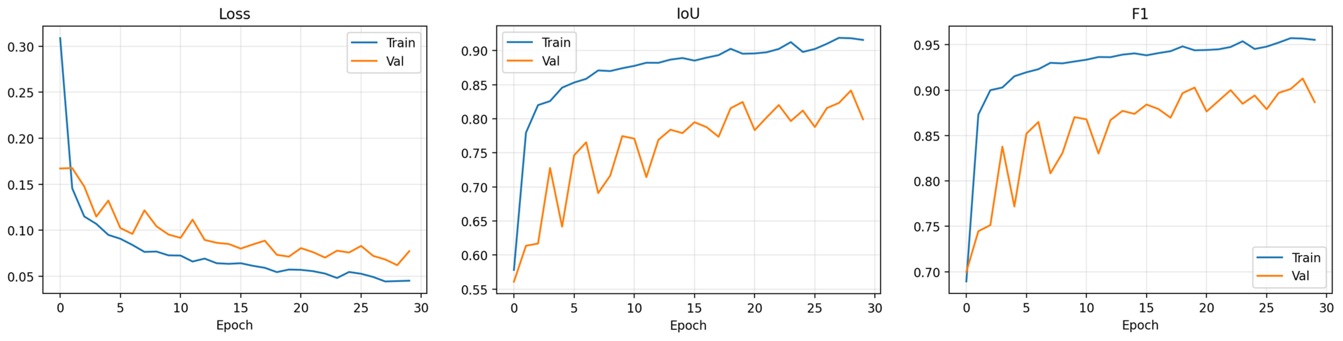
Figure 2 shows the training and validation loss, IoU and F1-score over 50 epochs. Loss curves for both training and validation show a close match throughout, with a steady and smooth decrease with no signs of overfitting. The model has a validation loss at epoch 48 of 0.0081, which is the lowest loss value in the validation set. Both IoU and F1 increase quickly during the first 15 epochs and start to converge slowly towards their maximum values.
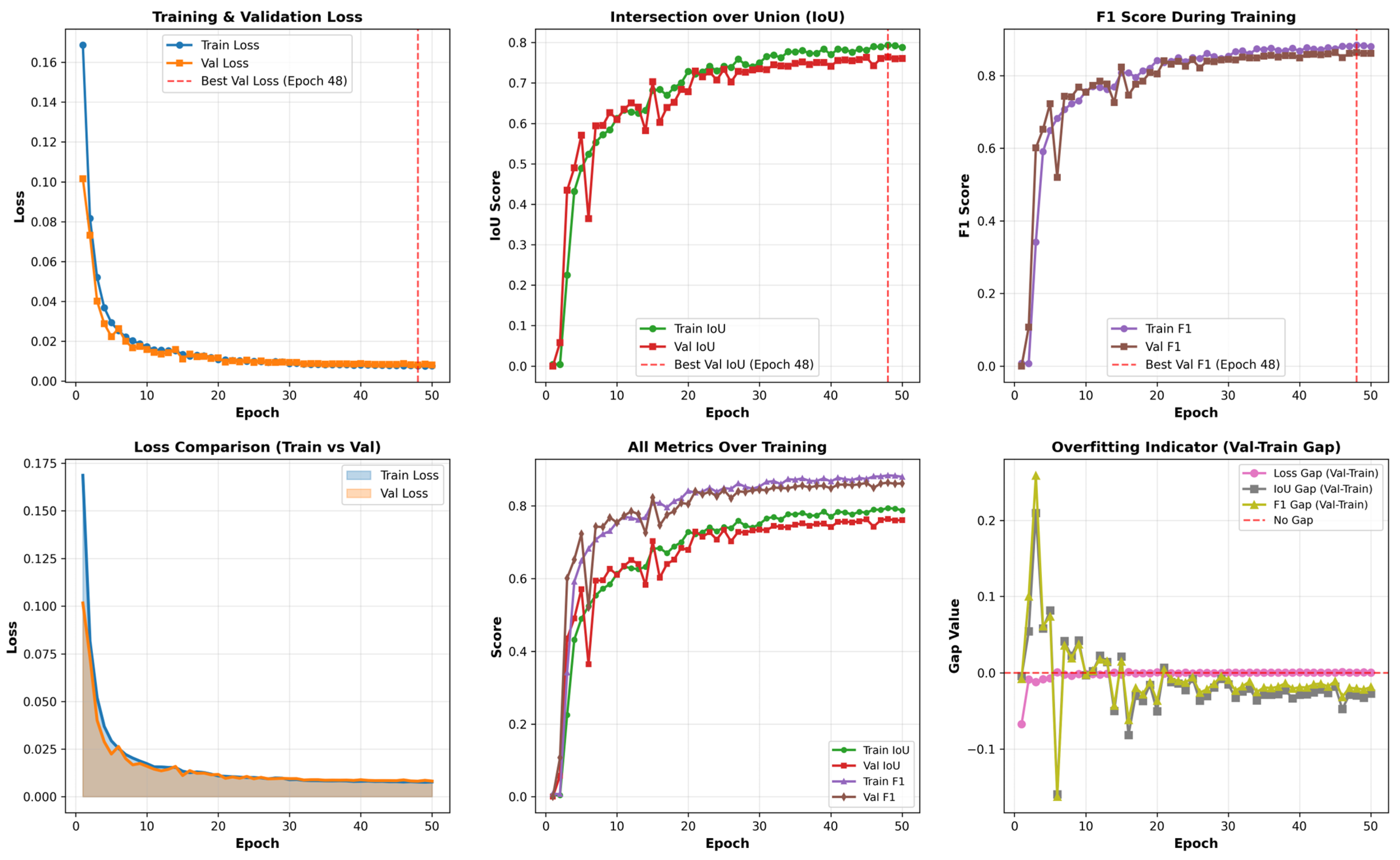
Figure 3 is a detailed analysis of training history shown in six panels. The figure at the top displays individual loss, IoU and F1. The bottom row displays the filled loss comparison, the combined metric overlay and the Val–Train gap (overfitting indicator). The overfitting indicator panel shows that the gaps between the actual and the “Val” remain low across all three metrics, and do not grow apart, which shows that generalization is stable.

4.2. Quantitative Performance on LEVIR-CD Test Set

All evaluation metrics are shown in Table 2, calculated on the test set of LEVIR-CD (128 image pairs, 67,108,864 total pixels). This is a desirable measure of accuracy, but the overall accuracy of CTA-Net is 98.99%, which is misleading due to the high number of unchanged pixels. The change class precision of 90.67% and recall (sensitivity) of 84.87% yield an F1-score of 87.68%, with an IoU of 78.06%. In the no-change class, the network predicts it with almost perfect precision (99.34%) and recall (99.62%) showing that it is not falsely predicting a change where there is not one.
Cohen’s kappa of 0.8715 is ‘almost perfect’ agreement with the ground truth beyond chance [45] and MCC of 0.8721 is a balanced measure that takes into account all four cells in the confusion matrix. A low FPR of 0.38% confirms a lack of erroneous identification of large areas of no change, which is essential for the operation of monitoring to prevent alert fatigue. The FNR of 15.13% represents the main remaining challenge: the model fails to detect about one changed pixel out of seven. This implies that low spectral contrast in small isolated buildings or buildings with low contrast between the pre- and post-change images are still difficult.

4.3. Confusion Matrix Analysis

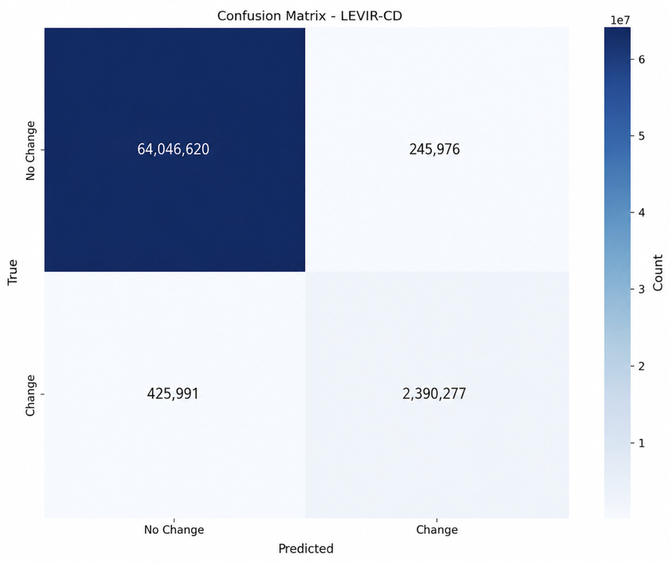
The pixel-wise confusion matrix is presented in Figure 4. Of the 2,816,268 changed pixels, 2,390,277 (84.87%) are correctly detected as true positives, while 425,991 are missed (false negatives). The 64,292,596 unchanged pixels are classified as true negatives; 64,046,620 of them (99.62%) are correctly classified and 245,976 are misclassified as false alarms.

4.4. ROC and Precision–Recall Analysis

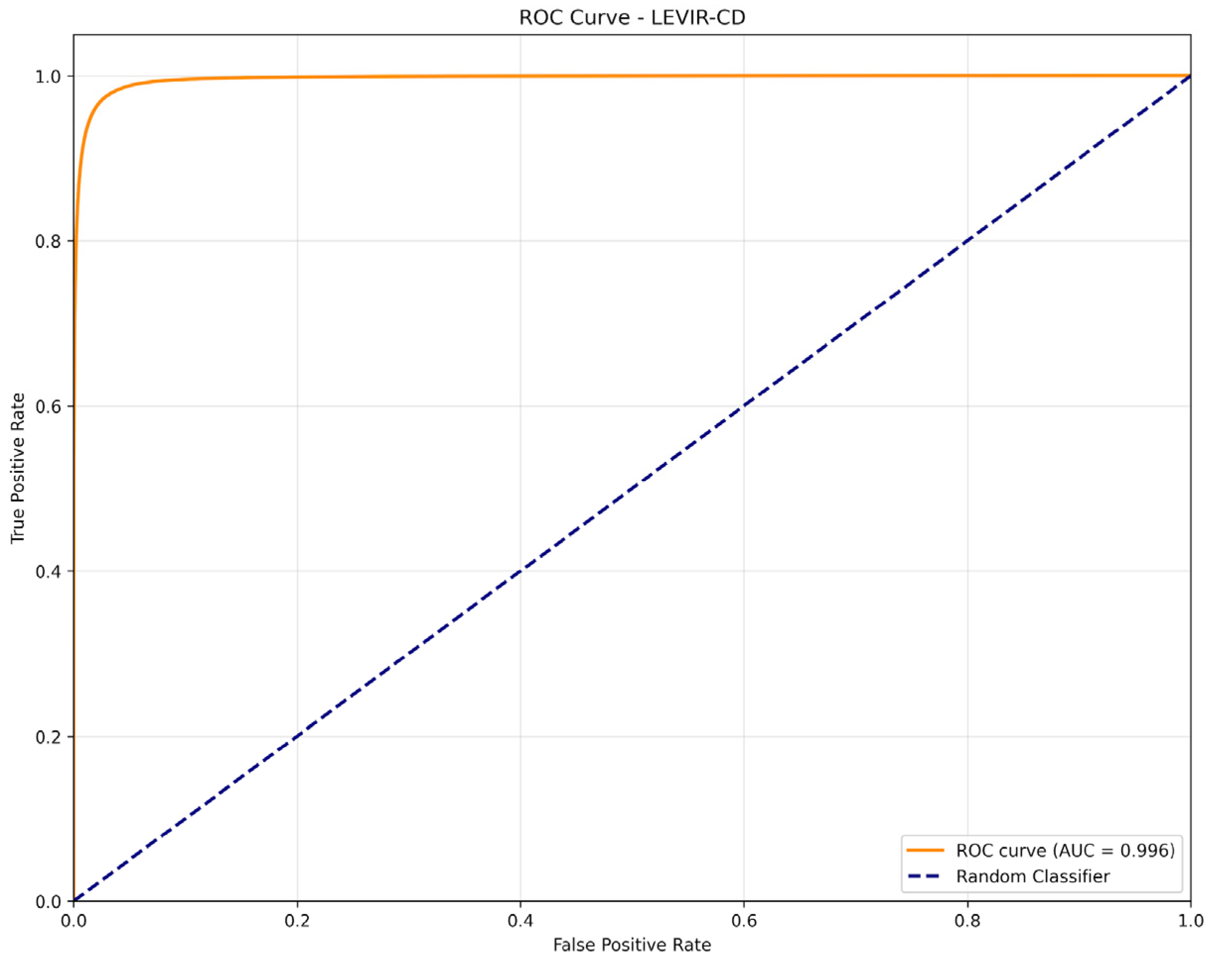
The ROC curve of the change class on the LEVIR-CD test set is shown in Figure 5. The AUC value of CTA-Net is 0.996. The curve is steeply ascending towards the upper left corner: the true positive rate is about 0.97 when the FPR is <0.02 and is near 1.0 at all FPR levels thereafter. This shape indicates that the model has very good separation of the change and no-change classes at almost all classification thresholds, and only slight degradation at the most aggressive extreme low-FPR threshold where the decision boundary is the most conservative.
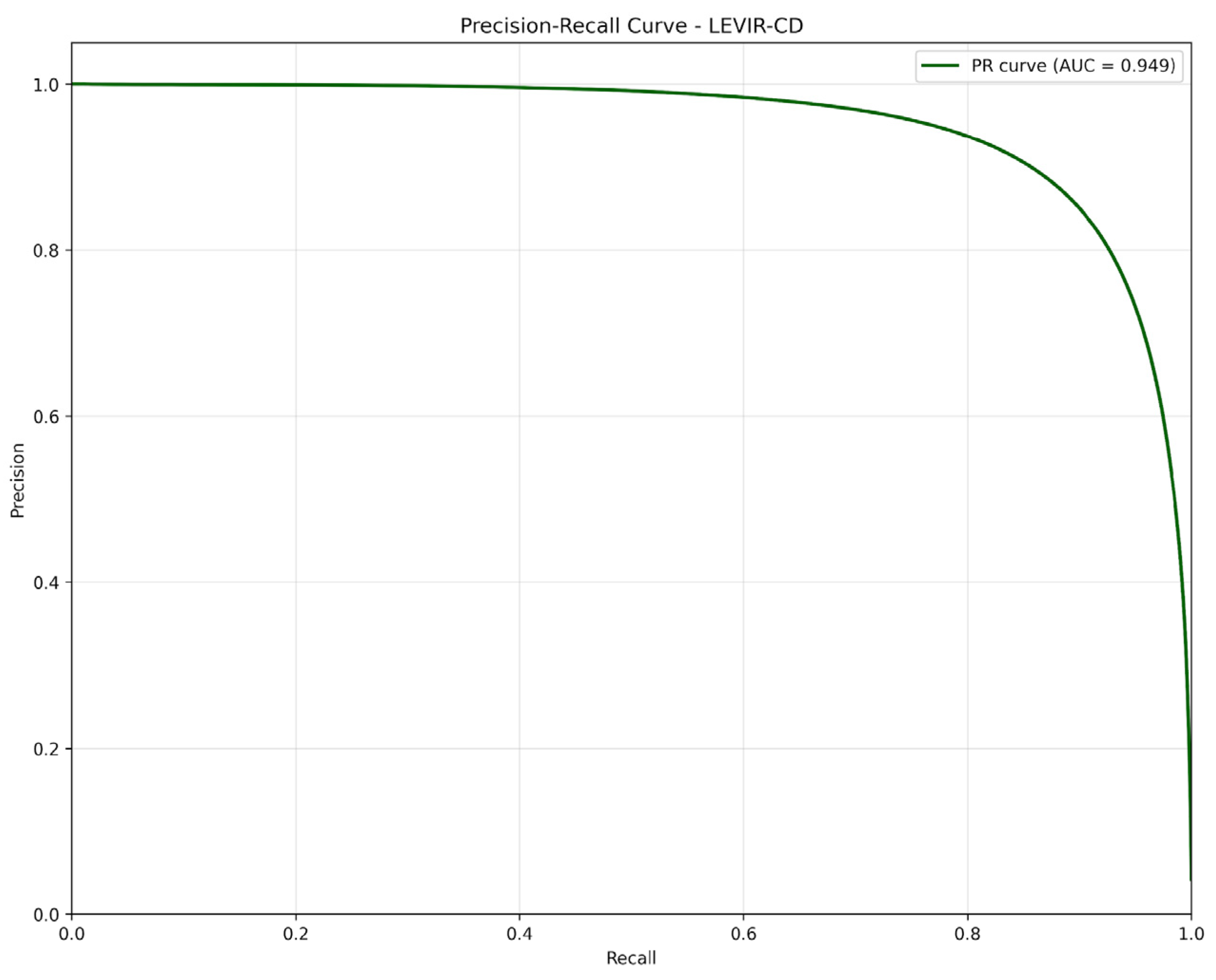
The precision–recall curve for the change class is displayed in Figure 6 and provides more informative curves when there is class imbalance. The curve also has an AUC of 0.949, which shows that precision is kept around 1.0 for most of the range of recall values with a small drop at the extreme values, thus performance is stable on the minority class.
The discrimination performance of both curves is satisfactory and both curves have stable performance across the entire range of classification thresholds. The ROC curve shows that the model has a high true positive rate and a low false positive rate, while the precision–recall curve shows that it achieves high precision at a broad range of recall values, even in the presence of class imbalance. The overall results show that the CTA-Net is able to classify the change and no-change class correctly and is robust to the varying thresholds.

4.5. Comparison with State-of-the-Art Methods

Table 3 lists some of the state-of-the-art methods evaluated on LEVIR-CD and compares them with CTA-Net. All comparisons made should be viewed with caution as the number of different evaluation protocols reported in the literature is numerous (some at the image patch level, others at the full 1024 × 1024 resolution) and the numerical values reported are from the original publications.
The inclusion of recent methods published between 2023 and 2024 confirms that CTA-Net remains competitive while maintaining a significantly lower parameter count (∼1.2 M) than comparable recent methods such as USSFC-Net, VcT, and HANet, making it particularly suitable for resource-constrained deployment scenarios.
When benchmarked against the compared methods, CTA-Net achieves the highest overall accuracy, and when benchmarked with other transformer-based methods, CTA-Net achieves a similar F1-score, while having a significantly lower number of parameters than these comparison methods. CTA-Net performs better than all the other baselines in terms of precision (90.67%) except for ChangeFormer, with a recall of 84.87%, which explains that the task of finding all changed pixels is difficult with the current training setup in absence of data augmentation. While transformer-based methods such as ChangeFormer [36] and HANet [47] achieve marginally higher F1-scores in this comparison, CTA-Net offers a substantially more lightweight (∼1.2 M parameters) and interpretable alternative, with attention maps explicitly grounded in quantified temporal difference rather than learned implicitly through self-attention.

4.6. Ablation Study

We perform an ablation study on the LEVIR-CD test set to measure the contribution of each component. The four model variants are compared: (i) a baseline Siamese U-Net without CTA modules or confidence head; (ii) the baseline with CTA modules only; (iii) the baseline with the confidence estimation head and hybrid loss only; and (iv) the full CTA-Net. The results are summarized in Table 4. The findings show that all components have positive impacts on the overall performance. The CTA modules improve the F1-score by 2.73 percentage points compared to the baseline, which again indicates that change discrimination is improved when using CTA modules. The benefit of uncertainty-aware optimization is captured with the confidence head with hybrid loss, which provides an additional 1.01 points advantage compared to the baseline. The proposed complementary components result in the best F1-score of 87.68% and IoU of 78.06% for the full CTA-Net, which confirms the complementary nature.

4.7. Qualitative Results

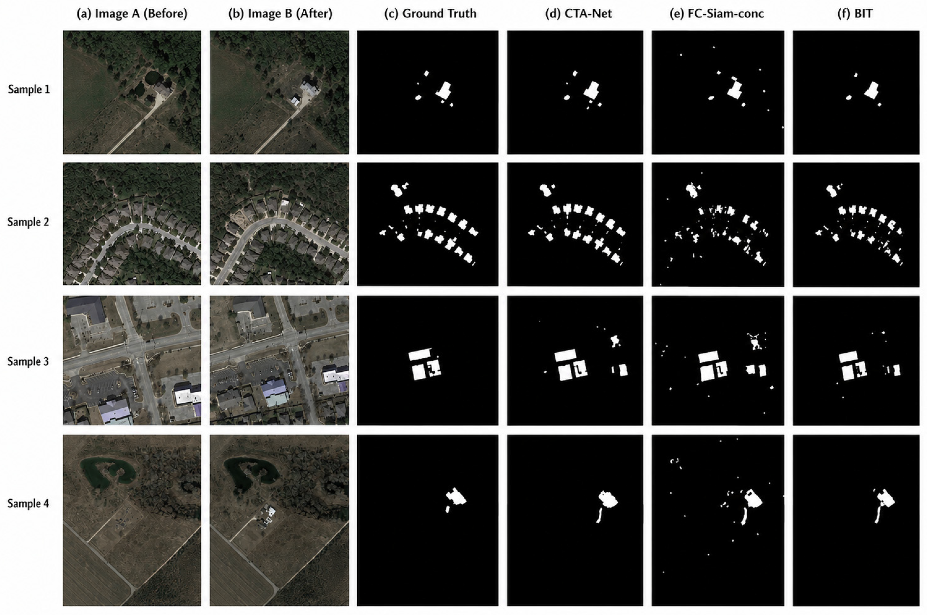
The qualitative change detection results of four test image pairs which were randomly selected are presented in Figure 7. For each panel, the first picture is the pre-change image, the second picture is the post-change image, the third picture is the ground truth mask, the fourth picture is the CTA-Net prediction, the fifth picture is the FC-Siam-conc prediction, and the sixth image is the BIT prediction. The CTA-Net algorithm yields a cleaner building boundary and fewer false positive results than FC-Siam-conc, and comparable boundary delineation as BIT, but with far fewer parameters. Furthermore, two failure scenarios are noted: false negative due to low spectral contrast of a newly built structure, and false positive due to seasonal variation in vegetation changing the spectral features to a similar magnitude as real spectral change.

4.8. The Multi-Scale Feature Response Visualizations

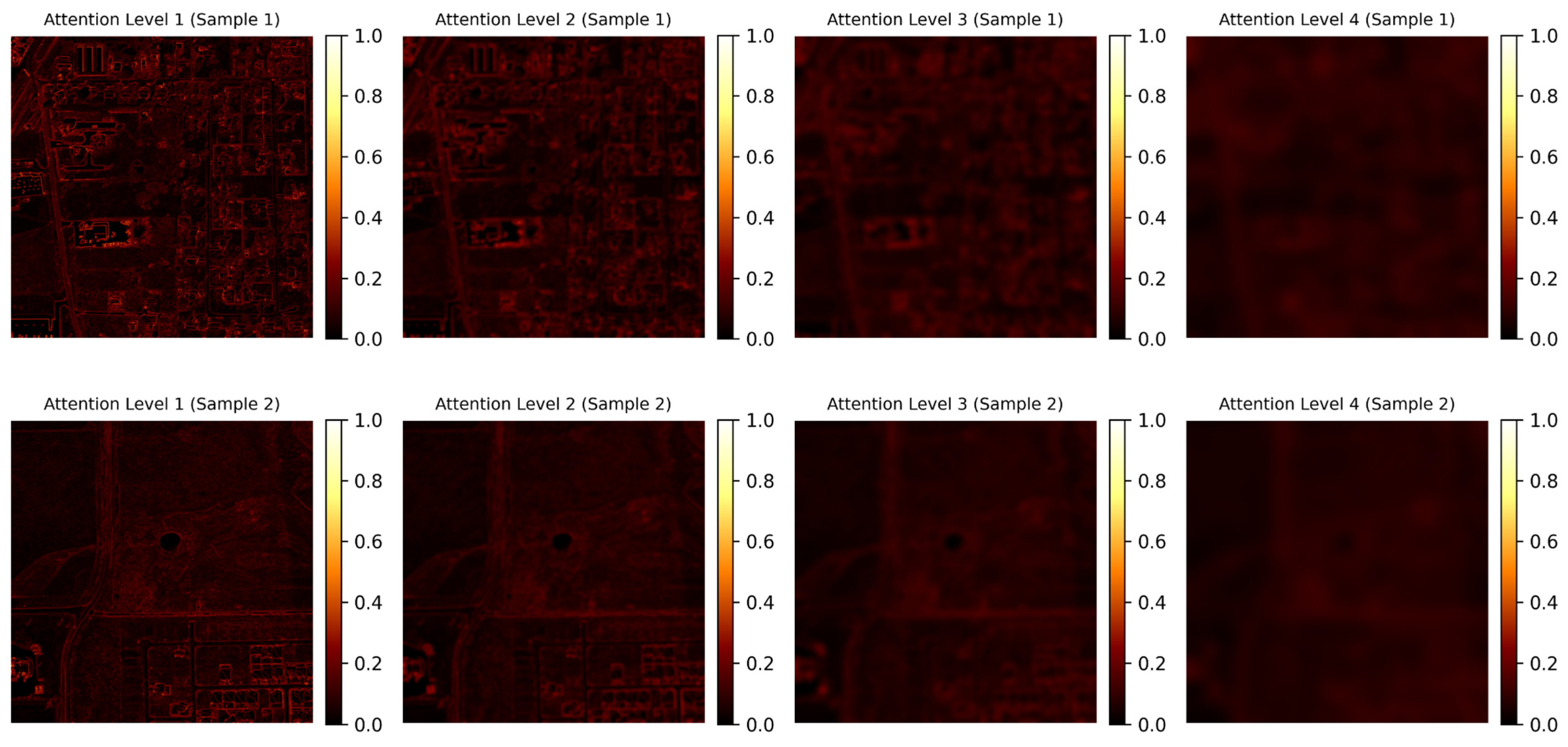
The multi-scale feature response visualizations in Figure 8 illustrate two representative samples from LEVIR-CD. The visualizations show the layers of feature extraction, from low-level visual elements to high-level semantic ones, and how the information in the image is represented at each. Brighter areas are related to more robust feature activation, as they are areas that make a stronger contribution to the learned representation.
In the case of level 1, the feature responses retain the finer spatial detail (boundary of buildings, roads, field edges, etc., and other high-frequency features). These are local texture and geometric properties that are relevant to accurate localization of an object. The feature representations at levels 2 and 3 are more abstract, combining neighbouring features together and less sensitive to fine-scale variations and image noise. This makes larger, spatial structures and contextual relationships stand out more.
Level 4 responses show a very smooth texture and mostly represent general scene-level features rather than specific objects. This behaviour is a gradual upscaling of receptive field sizes which enables the network to learn high-level semantic context and long-range spatial relationships. Turning from fine-scale local responses to coarse-scale semantic representations illustrates the capacity of the feature extraction process to be able to simultaneously model fine-scale structural information and global scene context.
The visualizations suggest that the network learns feature representations at multiple spatial scales and that the learned representations allow efficient characterization of objects in local regions and contextual patterns in broader, remote sensing images.

4.9. Confidence and Calibration Analysis

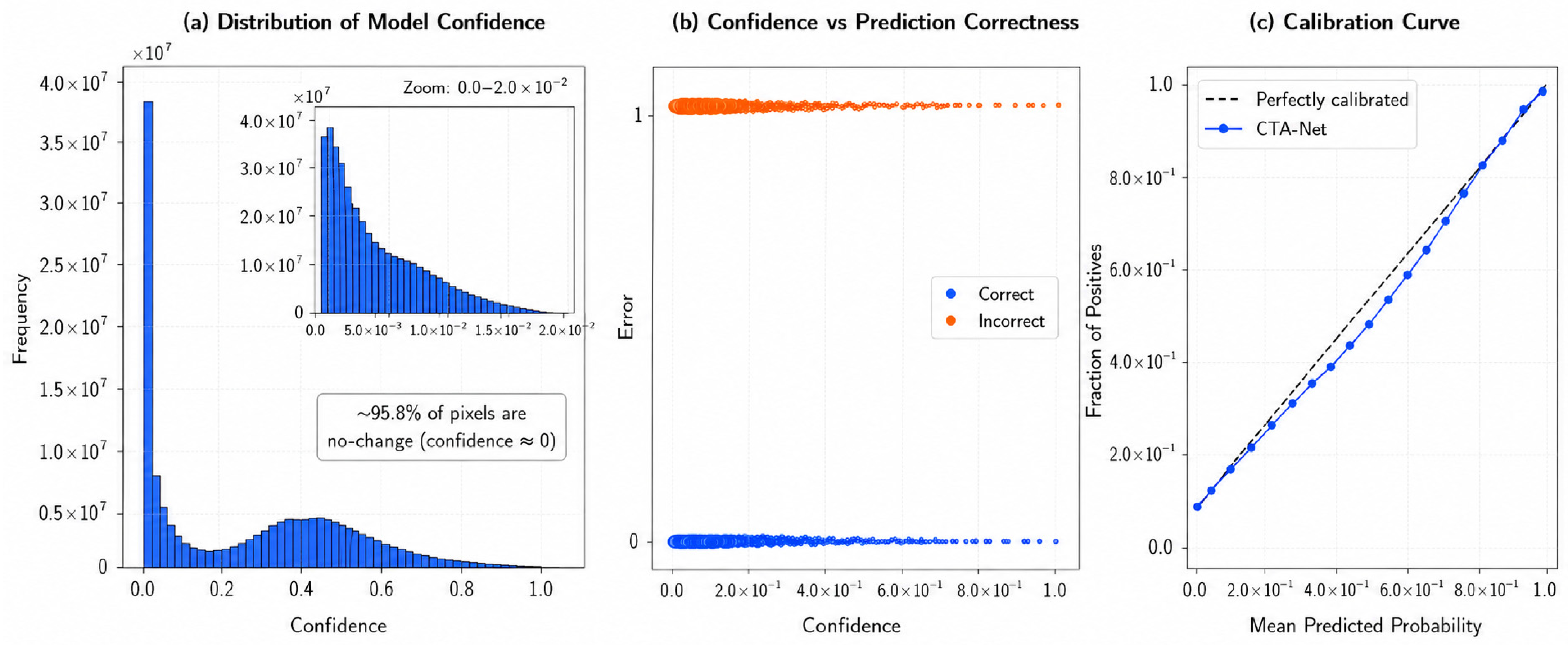
Three plots are shown in Figure 9: the model confidence distribution, a scatter plot of model confidence against the correct prediction, and the calibration curve. The confidence distribution has two modes, a large mode at 1.0 for the majority (unchanged) class, and a smaller mode for the (changed) class. We observe that the plot of the confidence (Figure 9a) shows raw output numbers of the confidence head with a sigmoid activation function. The extreme class imbalance is apparent in the LEVIR-CD, with the majority of the pixels at the extreme end of the class having values close to zero, about 95.8% of all pixels. The confidence head is trained to give low raw confidence scores to the majority class, resulting in a distribution that has a strong bias towards zero. The horizontal axis is properly scaled for the entire range [0, 1] and the apparent density around zero is related to the class distribution and not a numerical error. The calibration curve demonstrates that the CTA-Net is well calibrated, as the curve is fairly level with predicted probabilities closely approximating the empirical proportion of positives throughout the range of probabilities. A slightly underconfident behaviour is noted when the probability values are in between 0.3 and 0.7, with the empirical proportion of positives marginally exceeding the predicted probability in this range. This is consistent with the conservative confidence estimates observed for the majority class and with the model’s higher false negative rate (15.13%, Table 2), suggesting the model is generally cautious rather than overconfident in its predictions. Temperature scaling [48] may be used to further enhance calibration in future work. The same ideas of uncertainty-aware prediction and reliability estimation have been shown in related safety-critical areas like power infrastructure monitoring [49].

4.10. Transfer Learning Case Study: Agricultural Change Detection on Sentinel-2

For evaluation of cross-domain transferability of CTA-Net, a fine-tuning test was performed on multispectral Sentinel-2 data for agricultural fields. Compared to LEVIR-CD, this domain has three differences: firstly, the modality of the sensor used (11-band multispectral UINT16 vs. 3-band RGB optical); secondly, the semantics of the target (crop-cover change vs. building construction/demolition); and thirdly, the resolution of the spatial data (10–20 m vs. 0.5 m GSD).
The number of image pairs was increased to 94 (six geographic regions and 15 years) and tiled into 512 non-overlapping 256 × 256 patches (416 train/48 validation/48 test). The 1–4 regions (up to eight pairs per region) were used for training purposes, region 5 (four pairs) for validation purposes and region 6 (four pairs) for testing purposes. The binary change masks were automatically created using NDVI-delta thresholding, which was then applied uniformly in each split. A major constraint on the Sentinel-2 experiment was the same procedure for generating the training labels and test evaluation masks, based on the NDVI-delta thresholding. We point out that this supervision plan also makes use of a methodological limitation, namely that both training targets and the test assessment masks are based on the same NDVI-delta approach. As a result, metrics reported reflect the accuracy of the model’s approximation of the mask generation algorithm, but not necessarily its agreement with the true ground truth, which has been independently annotated. Therefore, this experiment should be seen as a proof-of-concept feasibility demonstration of transfer learning in agricultural change detection and not as a yardstick for the accuracy of the change detection results. Further work in validating with manually annotated maps or third-party labelled change maps would be useful.
The CTA-Net encoder input was adjusted to take in 11 channels of input. All but the last layer, enc1.conv, were found to be pre-trained on LEVIR-CD with a different channel size, so they were transferred. All other learned representations from the LEVIR-CD checkpoint were kept, including the encoder, attention, decoder and head weights.
Optimized AdamW on an initial learning rate of 5 × 10 4 , weight decay 10 5 , a ReduceLROnPlateau scheduler (patience 3 and factor 0.5), and early stopping (patience 7 and max epochs 30) and with L2-norm gradient clipping of 1.0. The loss function used the same formulation as before, that is the 0.7/0.3 mixing ratio BCE loss function. Random horizontal/vertical flip and rotation by 90° augmentation to training images.
Test-set performance on held-out region 6 is given in Table 5. The results suggest that despite variations in both semantic definition of change and spatial resolution in CTA-Net’s input sensory data, it displays stable predictive behaviour post domain transfer, even when the dimensionality differs between the two.
Under the supervision protocol NDVI-delta, the fine-tuned model is able to reach an IoU of 90.81% and an F1 of 95.18% on the agricultural test set. As the class balance in the domain of agriculture has been redistributed, precision and recall are almost equal (94.94% and 95.42% respectively), suggesting that the loss function based on confidence weights is well-balanced in both false positive and false negative cases. These are not compared directly to LEVIR-CD as various experiments have different domains, resolutions, sensors and supervision sources, so that a numerical comparison between experiments is not informative.
In order to successfully adapt to this change, only the input projection layer needed to be changed while all subsequent layers kept the same, which indicates that the Cross-Temporal Attention may be universalizable across different types of sensors under input normalization. Further validation in different areas of the world, across other sensors and with other independently annotated datasets would be needed to validate this property.

5. Discussion

This section discusses the design decisions made for CTA-Net and how these influence the model performance, interpretability and generalization. The previous section presented empirical results demonstrating that the approach proposed in this paper was effective, but in this section we aim to explain why the model works well and where it fails. We further investigate Cross-Temporal Attention for feature learning, the optimization effect of the confidence-weighted loss, and the compression-versus-detection trade-off. This information is then applied to uncover barriers to success and galvanize the path forward for improvement.

5.1. Effect of Cross-Temporal Attention

In CTA-Net, the design principle is that the L2 temporal difference magnitude is used as the input of the spatial attention instead of processing each temporal frame independently. This formulation makes the attention maps change-driven in that regions with high temporal feature difference will get high gate values, while regions that are stable are actively suppressed. The network therefore prioritizes the representation of meaningful changes, rather than redundantly representing the unchanged background information.
CTA modules are used in the multi-scale application, which reinforces this behaviour. The attention mechanism is able to extract fine-grained boundary information at lower encoder levels (levels 1–2), which facilitates accurate delineation of building edges. At higher levels (levels 3–4) it reacts to the larger structural patterns such as whole building blocks or changes in the urban structure. This hierarchical response follows the principles of multi-scale feature learning in a convolutional network, and visualizations of the attention of the network in Figure 8 confirm this.
The proposed method is a deliberate simplification compared to full cross-attention mechanisms as used in [33,35,50] and later in transformer-based change detection models, such as in [22,36]. In addition to not comparing pairwise tokens and having quadratic complexity, CTA-Net also significantly reduces the amount of computation, while still being able to capture the most informative discrepancies in the temporal data. In such a sense, the model takes a pragmatic “golden” path between the early Siamese differencing approaches and the deep transformer.
This design has some drawbacks, though. The magnitude of temporal difference is the most important factor in attracting attention, so that small or low contrast differences might not elicit a strong response, resulting in the false negative results that were observed. Also, there is no long-range dependency modelling representation that is explicit, so only implicitly globally distributed contextual relationships are captured by convolutional receptive fields. Despite these considerations, the proposed Cross-Temporal Attention mechanism proves itself to be an effective and computational efficient solution to high-resolution change detection tasks.

5.2. Impact of Confidence-Weighted Loss

The confidence head with its related weighted loss brings an adaptive learning mechanism, which changes during training. If the model’s prediction is vague and the confidence values are more or less equal in the early stages, the loss is more or less similar to the focal binary cross-entropy loss proposed in [42]. This is to ensure stable initial optimization and avoiding overemphasis on unreliable predictions. The confidence estimates gradually start to influence the loss more and more as the training continues and the model becomes more confident, thereby gradually changing the learning focus from uninformative to informative samples.
This behaviour might be viewed as a means of implicit curriculum learning, as the model slowly shifts focus to the more difficult and meaningful examples. The correct predictions with high confidence are reinforced, which leads to convergence and stabilizes decision boundaries. Concurrently, there is a greater penalty for the incorrect predictions when they have high confidence, which acts as a built-in hard negative mining strategy. This is especially relevant in the context of change detection problems, where the ambiguities of the boundaries between the classes and the imbalance in their distribution can cause misclassification that can be ignored by standard loss functions [1,17].
Another benefit of this formulation is that it is robust to noisy or imperfect annotations. In real remote sensing data, label noise often occurs from co-registration errors, seasonal variations, and arbitrary boundaries. The model can down-weight areas of uncertainty while emphasizing and focusing on patterns that are persistent, without being explicit about it, which enhances generalization. This is in line with the uncertainty-aware learning literature, e.g. [37,51], which highlights prediction reliability as well as accuracy.
The usefulness of this mechanism relies on the quality of the learned confidence estimates, however. A miscalibrated confidence head can lead to an over-amplification of noise in predictions or downplay of gradients. The confidence-weighted loss offers a principled and efficient approach to optimize in imbalanced and noisy change detection settings.

5.3. Strengths and Limitations

CTA-Net shows a good compromise between performance, efficiency and interpretability. The model is very effective due to its relatively small number of parameters (∼1.2 M) in comparison with transformer-based models like [22,36] that often demand much larger models and higher computational capacity. The Cross-Temporal Attention mechanism allows the network to specifically attend to regions of change, and the lightweight convolutional backbone makes it more practical to deploy. Furthermore, the model is somewhat transparent, with maps of the participants’ attention, thus making it possible to inspect the decision-making processes visually, and is reasonably calibrated in terms of confidence estimates, which are useful for real-world applications. The model’s performance remained stable during training for 50 epochs or more, and its performance was not significantly affected by the choice of hyperparameters, indicating its robustness and usability.
Meanwhile, there are some weaknesses associated with the experimental analysis. A false negative rate of 15.13% shows that the model is not performing well on detecting small scale changes and objects with low spectral contrast, which is also previously reported in the literature [1,18]. This indicates that the attention mechanism is successful in reducing false positives but could fail to capture fine-grained variations that do not result in significant feature differences. Moreover, the existing design only considers two-temporal input and fails to take advantage of richer temporal context found in multi-temporal sequences, which has been demonstrated to be advantageous for robustness in dynamic environments [52,53,54].
It is important to mention that most of the CTA-Net components are based on existing mechanisms in the literature. The spatial attention branch is based on ideas similar to CBAM [32] and the channel attention branch is based on an SE-style recalibration approach [34], and the general principle of guiding attention with temporal difference features has been explored in prior work. We do not claim novelty in the use of difference-guided attention as a general strategy. Rather, the specific contribution of CTA-Net lies in three concrete design choices: (i) a cascaded rather than parallel attention structure, in which channel attention A c (Equation (8)) is computed from the spatially gated feature F (Equation (7)) rather than independently from the raw difference signal, allowing channel recalibration to operate on an already spatially refined representation; (ii) the consistent application of this cascaded difference-guided attention at every encoder scale (Equations (5)–(9), applied at levels 1–4), producing the hierarchical fine-to-coarse attention behaviour visualized in Figure 8, rather than restricting attention to a single scale or the bottleneck only; and (iii) achieving this with a substantially smaller parameter budget (∼1.2 M) than comparable difference-aware or transformer-based methods such as USSFC-Net, VcT, and HANet, as shown in Table 3. These are incremental rather than fundamental architectural contributions, and we have revised the text to avoid overstating the novelty of the underlying attention mechanism itself. Similarly, the confidence estimation head does not give the same level of certainty as more sophisticated uncertainty estimation methods like deep ensembles, Monte Carlo dropout or Bayesian neural networks [37,51]. These are worthwhile avenues for further research.
The other drawback of this experimental approach is that this one does not include any data enhancement during training. This approach was taken because it allows the effects of the proposed architecture to be isolated and a controlled baseline evaluation can be carried out, but it may lead to conservative performance estimates when compared to the use of more extensive augmentation strategies. Some of these techniques have been demonstrated to enhance robustness and generalization in remote sensing applications including random flipping, rotation, scaling and colour perturbation [55]. The result should not be directly compared with methods that are trained with strong augmentation pipelines. In future work, a systematic exploration of augmentation strategies will be conducted and will be explored in relation to the proposed Cross-Temporal Attention mechanism.

5.4. Future Work

There are multiple directions of potentially improving the performance of CTA-Net and making it applicable to a larger problem set. First, it is expected that simply adding common data augmentation techniques [55] like random rotation, flipping, scaling, and random colour jittering will increase robustness and improve recall, especially in difficult cases where the viewpoints differ or the seasons are not aligned. These methods have been used in contemporary remote sensing pipelines and can improve the generalization of the various datasets.
Second, being able to extend this architecture from bi-temporal inputs to multi-temporal sequences ( T > 2 ) is an interesting direction for future study. The extra temporal observations enabled the model to describe change trajectories as opposed to just pairwise differences, which allowed for better identification of gradual or complex changes. This is consistent with the recent push in temporal modelling for remote sensing analysis for richer temporal context, which have been demonstrated to perform better in dynamic environments.
Third, pre-trained backbones like ResNet-50 [56] trained on large-scale datasets like ImageNet could be incorporated into the current lightweight encoder to improve its performance. Such transfer learning strategies have been shown to be consistently effective in denoting the quality of the representation of the features in vision tasks such as change detection, while keeping computational overheads manageable.
Fourth, adding multi-scale deep supervision (with auxiliary prediction heads at intermediate decoder layers) can enhance gradient propagation and induce more precise localization of changes at various spatial scales. It has worked well in encoder–decoder networks like fully convolutional networks for semantic segmentation and is expected to work well for fine-grained building change delineation network variants like UNet [57].

6. Conclusions

In this work, a Cross-Temporal Attention Network (CTA-Net) for binary change detection for bi-temporal remote sensing images is presented. The proposed model features a shared Siamese encoder, multi-scale Cross-Temporal Attention mechanisms, and a confidence-aware learning strategy, which enables the model to handle pseudo-changes caused by illumination changes, seasons, and sensor noise. The experimental results achieved on the LEVIR-CD dataset show that the CTA-Net has a high accuracy with good precision/recall ratio and stable convergence without overfitting. Further, qualitative analysis is conducted and results show that the model is able to generate well calibrated probabilistic output and interpretable attention maps, which further validates the suitability of the model for practical applications.
To further explore the generalization capability, a multispectral transfer learning case study was carried out on Sentinel-2 agriculture images. The model was successfully adopted to a higher-dimensional input space with a small number of architectural changes, just in the first projection layer. Fine-tuning results show that CTA-Net can successfully transfer learnt representations across sensor modalities, spatial resolution and semantic domain. However, because of the reliance on NDVI-delta thresholding for training and evaluation, the reported performance is consistent with the pseudo-labelling idea, not agreement with an independent set of annotations for the ground truth. Therefore, this experiment can be considered a proof-of-concept test of the cross-domain adaptability.
In change detection, CTA-Net offers a powerful and interpretable framework that strikes a balance between performance and model complexity. Further research will be directed towards validation with manually annotated or third-party datasets, the extension of the approach to multi-class and multi-temporal change detection problems, and the enhancement of robustness under weak and noisy supervision. Future directions involve investigating domain adaptation methods, incorporating self-supervised pre-training, and testing the performance on a broader sensor and geographic domain to further validate the model’s generalization ability.

Author Contributions

Conceptualization, A.S. and F.A.; methodology, A.S.; software, F.A.; validation, M.A., V.S. and G.N.; formal analysis, M.A.; investigation, V.S.; resources, G.N.; data curation, F.A.; writing—original draft preparation, A.S.; writing—review and editing, A.S. and M.A.; visualization, V.S.; supervision, A.S.; project administration, F.A.; funding acquisition, F.A. All authors have read and agreed to the published version of the manuscript.

Funding

This research has been funded by the Committee of Science of the Ministry of Science and Higher Education of the Republic of Kazakhstan (grant No. BR28713375 ‘Multipurpose Robotic UAV Platform for Remote Monitoring (AeroScope)’).

Institutional Review Board Statement

Not applicable.

Informed Consent Statement

Not applicable.

Data Availability Statement

The data used in this study are publicly available and were obtained from the LEVIR-CD dataset [40], which is a benchmark dataset for building change detection in very-high-resolution remote sensing imagery. The dataset contains 637 pairs of 1024 × 1024 RGB images collected from Google Earth over 20 regions in Texas, USA, with a ground sampling distance of 0.5 m and temporal intervals ranging from 5 to 14 years. The dataset includes pixel-level binary change masks indicating newly constructed and demolished buildings. The dataset is publicly accessible at: https://justchenhao.github.io/LEVIR/ (accessed on 14 May 2026) (originally introduced in Chen and Shi [40], Remote Sensing, 2020, 12, 1662, DOI: 10.3390/rs12101662).

Conflicts of Interest

The authors declare no conflicts of interest.

References

  1. Shi, W.; Zhang, M.; Zhang, R.; Chen, S.; Zhan, Z. Change Detection Based on Artificial Intelligence: State-of-the-Art and Challenges. Remote Sens. 2020, 12, 1688. [Google Scholar] [CrossRef]
  2. Cheng, G.; Huang, Y.; Li, X.; Lyu, S.; Xu, Z.; Zhao, Q.; Xiang, S. Change Detection Methods for Remote Sensing in the Last Decade: A Comprehensive Review. arXiv 2023, arXiv:2305.05813. [Google Scholar] [CrossRef]
  3. Ding, L.; Hong, D.; Zhao, M.; Chen, H.; Li, C.; Deng, J.; Yokoya, N.; Bruzzone, L.; Chanussot, J. A Survey of Sample-Efficient Deep Learning for Change Detection in Remote Sensing. arXiv 2025, arXiv:2502.02835. [Google Scholar] [CrossRef]
  4. Basavaraju, K.S.; Sravya, N.; Kevala, V.D.; Lal, S. Recent Advances in Urban Expansion Monitoring Through Deep Learning-Based Semantic Change Detection Techniques From Satellite Imagery. In 2024 IEEE Space, Aerospace and Defence Conference (SPACE); IEEE: Bangalore, India, 2024; pp. 169–173. [Google Scholar] [CrossRef]
  5. Gupta, R.; Goodman, B.; Patel, N.; Hosfelt, R.; Sajeev, S.; Heim, E.; Doshi, J.; Lucas, K.; Choset, H.; Gaston, M. xBD: A Dataset for Assessing Building Damage from Satellite Imagery. arXiv 2019, arXiv:1911.09296. [Google Scholar] [CrossRef]
  6. Hoekman, D.; Kooij, B.; Quiñones, M.; Vellekoop, S.; Carolita, I.; Budhiman, S.; Arief, R.; Roswintiarti, O. Wide-Area Near-Real-Time Monitoring of Tropical Forest Degradation and Deforestation Using Sentinel-1. Remote Sens. 2020, 12, 3263. [Google Scholar] [CrossRef]
  7. Drusch, M.; Del Bello, U.; Carlier, S.; Colin, O.; Fernandez, V.; Gascon, F.; Hoersch, B.; Isola, C.; Laberinti, P.; Martimort, P.; et al. Sentinel-2: ESA’s Optical High-Resolution Mission for GMES Operational Services. Remote Sens. Environ. 2012, 120, 25–36. [Google Scholar] [CrossRef]
  8. Ball, J.E.; Anderson, D.T.; Chan, C.S. Comprehensive Survey of Deep Learning in Remote Sensing: Theories, Tools, and Challenges for the Community. J. Appl. Remote Sens. 2017, 11, 042609. [Google Scholar] [CrossRef]
  9. Daudt, R.C.; Le Saux, B.; Boulch, A. Fully Convolutional Siamese Networks for Change Detection. In 2018 25th IEEE International Conference on Image Processing (ICIP); IEEE: Athens, Greece, 2018; pp. 4063–4067. [Google Scholar] [CrossRef]
  10. Bruzzone, L.; Prieto, D.F. Automatic Analysis of the Difference Image for Unsupervised Change Detection. IEEE Trans. Geosci. Remote Sens. 2000, 38, 1171–1182. [Google Scholar] [CrossRef]
  11. Johnson, R.D.; Kasischke, E.S. Change Vector Analysis: A Technique for the Multispectral Monitoring of Land Cover and Condition. Int. J. Remote Sens. 1998, 19, 411–426. [Google Scholar] [CrossRef]
  12. Singh, A. Digital Change Detection Techniques Using Remotely-Sensed Data. Int. J. Remote Sens. 1989, 10, 989–1003. [Google Scholar] [CrossRef]
  13. Bruzzone, L.; Prieto, D.F. An Adaptive Semiparametric and Context-Based Approach to Unsupervised Change Detection in Multitemporal Remote-Sensing Images. IEEE Trans. Image Process. 2002, 11, 452–466. [Google Scholar] [CrossRef] [PubMed]
  14. LeCun, Y.; Bengio, Y.; Hinton, G. Deep Learning. Nature 2015, 521, 436–444. [Google Scholar] [CrossRef] [PubMed]
  15. Long, J.; Shelhamer, E.; Darrell, T. Fully Convolutional Networks for Semantic Segmentation. In Proceedings of the IEEE Conference on Computer Vision and Pattern Recognition (CVPR), Boston, MA, USA, 7–12 June 2015; IEEE: Piscataway, NJ, USA, 2015; pp. 3431–3440. [Google Scholar] [CrossRef]
  16. Bromley, J.; Guyon, I.; LeCun, Y.; Säckinger, E.; Shah, R. Signature Verification Using a Siamese Time Delay Neural Network. Adv. Neural Inf. Process. Syst. 1994, 6, 737–744. [Google Scholar] [CrossRef]
  17. Bai, T.; Wang, L.; Yin, D.; Sun, K.; Chen, Y.; Li, W.; Li, D. Deep Learning for Change Detection in Remote Sensing: A Review. Geo-Spat. Inf. Sci. 2023, 26, 262–288. [Google Scholar] [CrossRef]
  18. Khelifi, L.; Mignotte, M. Deep Learning for Change Detection in Remote Sensing Images: Comprehensive Review and Meta-Analysis. IEEE Access 2020, 8, 126385–126400. [Google Scholar] [CrossRef]
  19. Zhu, X.X.; Tuia, D.; Mou, L.; Xia, G.-S.; Zhang, L.; Xu, F.; Fraundorfer, F. Deep Learning in Remote Sensing: A Comprehensive Review and List of Resources. IEEE Geosci. Remote Sens. Mag. 2017, 5, 8–36. [Google Scholar] [CrossRef]
  20. Lei, T.; Geng, X.; Ning, H.; Lv, Z.; Gong, M.; Jin, Y.; Nandi, A.K. Ultralightweight Spatial–Spectral Feature Cooperation Network for Change Detection in Remote Sensing Images. IEEE Trans. Geosci. Remote Sens. 2023, 61, 4402114. [Google Scholar] [CrossRef]
  21. Zhao, X.; Zhao, K.; Li, S.; Wang, X. GeSANet: Geospatial-Awareness Network for VHR Remote Sensing Image Change Detection. IEEE Trans. Geosci. Remote Sens. 2023, 61, 5402814. [Google Scholar] [CrossRef]
  22. Chen, H.; Shi, Z. Remote Sensing Image Change Detection with Transformers. IEEE Trans. Geosci. Remote Sens. 2022, 60, 5607514. [Google Scholar] [CrossRef]
  23. Zhang, C.; Yue, P.; Tapete, D.; Jiang, L.; Shangguan, B.; Huang, L.; Liu, G. A Deeply Supervised Image Fusion Network for Change Detection in High Resolution Bi-Temporal Remote Sensing Images. ISPRS J. Photogramm. Remote Sens. 2020, 166, 183–200. [Google Scholar] [CrossRef]
  24. Liu, Y.; Pang, C.; Zhan, Z.; Zhang, X.; Yang, X. Building Change Detection for Remote Sensing Images Using a Dual-Task Constrained Deep Siamese Convolutional Network Model. IEEE Geosci. Remote Sens. Lett. 2021, 18, 811–815. [Google Scholar] [CrossRef]
  25. Fang, S.; Li, K.; Shao, J.; Li, Z. SNUNet-CD: A Densely Connected Siamese Network for Change Detection of VHR Images. IEEE Geosci. Remote Sens. Lett. 2022, 19, 8007805. [Google Scholar] [CrossRef]
  26. Peng, D.; Bruzzone, L.; Zhang, Y.; Guan, H.; Ding, H.; Huang, X. SemiCDNet: A Semisupervised Convolutional Neural Network for Change Detection in High Resolution Remote-Sensing Images. IEEE Trans. Geosci. Remote Sens. 2021, 59, 5891–5906. [Google Scholar] [CrossRef]
  27. Shi, Q.; Liu, M.; Li, S.; Liu, X.; Wang, F.; Zhang, L. A Deeply Supervised Attention Metric-Based Network and an Open Aerial Image Dataset for Remote Sensing Change Detection. IEEE Trans. Geosci. Remote Sens. 2022, 60, 5604816. [Google Scholar] [CrossRef]
  28. Zhan, Y.; Fu, K.; Yan, M.; Sun, X.; Wang, H.; Qiu, X. Change Detection Based on Deep Siamese Convolutional Network for Optical Aerial Images. IEEE Geosci. Remote Sens. Lett. 2017, 14, 1845–1849. [Google Scholar] [CrossRef]
  29. Guo, E.; Fu, X.; Zhu, J.; Deng, M.; Liu, Y.; Zhu, Q.; Gong, H. Learning to Measure Change: Fully Convolutional Siamese Metric Networks for Scene Change Detection. arXiv 2018, arXiv:1810.09111. [Google Scholar] [CrossRef]
  30. Serek, A.; Amirgaliyev, B.; Li, R.Y.M.; Zhumadillayeva, A.; Yedilkhan, D. Crowd Density Estimation Using Enhanced Multi-Column Convolutional Neural Network and Adaptive Collation. IEEE Access 2025, 13, 146956–146972. [Google Scholar] [CrossRef]
  31. Chen, J.; Yuan, Z.; Peng, J.; Chen, L.; Huang, H.; Zhu, J.; Liu, Y.; Li, H. DASNet: Dual Attentive Fully Convolutional Siamese Networks for Change Detection in High-Resolution Satellite Images. IEEE J. Sel. Top. Appl. Earth Obs. Remote Sens. 2021, 14, 1194–1206. [Google Scholar] [CrossRef]
  32. Woo, S.; Park, J.; Lee, J.-Y.; Kweon, I.S. CBAM: Convolutional Block Attention Module. In Proceedings of the European Conference on Computer Vision (ECCV), 2018; Springer: Cham, Switzerland, 2018; pp. 3–19. [Google Scholar] [CrossRef]
  33. Vaswani, A.; Shazeer, N.; Parmar, N.; Uszkoreit, J.; Jones, L.; Gomez, A.N.; Kaiser, Ł.; Polosukhin, I. Attention Is All You Need. Adv. Neural Inf. Process. Syst. 2017, 30, 5998–6008. [Google Scholar] [CrossRef]
  34. Hu, J.; Shen, L.; Sun, G. Squeeze-and-Excitation Networks. In Proceedings of the IEEE Conference on Computer Vision and Pattern Recognition (CVPR), Salt Lake City, UT, USA, 18–23 June 2018; IEEE: Piscataway, NJ, USA, 2018; pp. 7132–7141. [Google Scholar] [CrossRef]
  35. Dosovitskiy, A.; Beyer, L.; Kolesnikov, A.; Weissenborn, D.; Zhai, X.; Unterthiner, T.; Dehghani, M.; Minderer, M.; Heigold, G.; Gelly, S.; et al. An Image Is Worth 16×16 Words: Transformers for Image Recognition at Scale. arXiv 2021, arXiv:2010.11929. [Google Scholar] [CrossRef]
  36. Bandara, W.G.C.; Patel, V.M. A Transformer-Based Siamese Network for Change Detection. In IGARSS 2022—2022 IEEE International Geoscience and Remote Sensing Symposium; IEEE: New York, NY, USA, 2022; pp. 207–210. [Google Scholar] [CrossRef]
  37. Gal, Y.; Ghahramani, Z. Dropout as a Bayesian Approximation: Representing Model Uncertainty in Deep Learning. In Proceedings of the 33rd International Conference on Machine Learning (ICML), New York, NY, USA, 19–24 June 2016; PMLR: Brookline, MA, USA, 2016; Volume 48, pp. 1050–1059. [Google Scholar] [CrossRef]
  38. Goodfellow, I.; Bengio, Y.; Courville, A. Deep Learning; MIT Press: Cambridge, MA, USA, 2016. [Google Scholar]
  39. Schmidhuber, J. Deep Learning in Neural Networks: An Overview. Neural Netw. 2015, 61, 85–117. [Google Scholar] [CrossRef] [PubMed]
  40. Chen, H.; Shi, Z. A Spatial-Temporal Attention-Based Method and a New Dataset for Remote Sensing Image Change Detection. Remote Sens. 2020, 12, 1662. [Google Scholar] [CrossRef]
  41. Cheng, G.; Han, J.; Lu, X. Remote Sensing Image Scene Classification: Benchmark and State of the Art. Proc. IEEE 2017, 105, 1865–1883. [Google Scholar] [CrossRef]
  42. Lin, T.-Y.; Goyal, P.; Girshick, R.; He, K.; Dollár, P. Focal Loss for Dense Object Detection. In Proceedings of the IEEE International Conference on Computer Vision (ICCV), Venice, Italy, 22–29 October 2017; IEEE: Piscataway, NJ, USA, 2017; pp. 2980–2988. [Google Scholar] [CrossRef]
  43. Milletari, F.; Navab, N.; Ahmadi, S.-A. V-Net: Fully Convolutional Neural Networks for Volumetric Medical Image Segmentation. In Proceedings of the Fourth International Conference on 3D Vision (3DV); IEEE: New York, NY, USA, 2016; pp. 565–571. [Google Scholar] [CrossRef]
  44. Loshchilov, I.; Hutter, F. Decoupled Weight Decay Regularization. arXiv 2019, arXiv:1711.05101. [Google Scholar] [CrossRef]
  45. Landis, J.R.; Koch, G.G. The Measurement of Observer Agreement for Categorical Data. Biometrics 1977, 33, 159–174. [Google Scholar] [CrossRef]
  46. Jiang, B.; Wang, Z.; Wang, X.; Zhang, Z.; Chen, L.; Wang, X.; Luo, B. VcT: Visual Change Transformer for Remote Sensing Image Change Detection. IEEE Trans. Geosci. Remote Sens. 2023, 61, 2005214. [Google Scholar] [CrossRef]
  47. Han, C.; Wu, C.; Guo, H.; Hu, M.; Chen, H. HANet: A Hierarchical Attention Network for Change Detection with Bitemporal Very-High-Resolution Remote Sensing Images. IEEE J. Sel. Top. Appl. Earth Obs. Remote Sens. 2023, 16, 3867–3878. [Google Scholar] [CrossRef]
  48. Guo, C.; Pleiss, G.; Sun, Y.; Weinberger, K.Q. On Calibration of Modern Neural Networks. In Proceedings of the 34th International Conference on Machine Learning (ICML), Sydney, NSW, Australia, 6–11 August 2017; PMLR: Brookline, MA, USA, 2017; Volume 70, pp. 1321–1330. [Google Scholar] [CrossRef]
  49. Afanaseva, O.V.; Tulyakov, T.F.; Shaimardanov, A.A. Deep Learning-Based Visual Analytics for Efficiency and Safety Optimization in Power Infrastructure. Eng 2026, 7, 135. [Google Scholar] [CrossRef]
  50. Wang, X.; Girshick, R.; Gupta, A.; He, K. Non-Local Neural Networks. In Proceedings of the IEEE Conference on Computer Vision and Pattern Recognition (CVPR), Salt Lake City, UT, USA, 18–23 June 2018; IEEE: Piscataway, NJ, USA, 2018; pp. 7794–7803. [Google Scholar] [CrossRef]
  51. Lakshminarayanan, B.; Pritzel, A.; Blundell, C. Simple and Scalable Predictive Uncertainty Estimation Using Deep Ensembles. In Advances in Neural Information Processing Systems (NeurIPS); Curran Associates, Inc.: Red Hook, NY, USA, 2017; Volume 30. [Google Scholar] [CrossRef]
  52. Li, Z.; Tang, C.; Wang, L.; Zomaya, A.Y. Remote Sensing Change Detection via Temporal Feature Interaction and Guided Refinement. IEEE Trans. Geosci. Remote Sens. 2022, 60, 5628711. [Google Scholar] [CrossRef]
  53. Papadomanolaki, M.; Vakalopoulou, M.; Karantzalos, K. A Deep Multitask Learning Framework Coupling Semantic Segmentation and Fully Convolutional LSTM Networks for Urban Change Detection. IEEE Trans. Geosci. Remote Sens. 2021, 59, 7651–7668. [Google Scholar] [CrossRef]
  54. Mou, L.; Bruzzone, L.; Zhu, X.X. Learning Spectral-Spatial-Temporal Features via a Recurrent Convolutional Neural Network for Change Detection in Multispectral Imagery. IEEE Trans. Geosci. Remote Sens. 2019, 57, 924–935. [Google Scholar] [CrossRef]
  55. Shorten, C.; Khoshgoftaar, T.M. A Survey on Image Data Augmentation for Deep Learning. J. Big Data 2019, 6, 60. [Google Scholar] [CrossRef]
  56. He, K.; Zhang, X.; Ren, S.; Sun, J. Deep Residual Learning for Image Recognition. In Proceedings of the IEEE Conference on Computer Vision and Pattern Recognition (CVPR); IEEE: Las Vegas, NV, USA, 2016; pp. 770–778. [Google Scholar] [CrossRef]
  57. Ronneberger, O.; Fischer, P.; Brox, T. U-Net: Convolutional Networks for Biomedical Image Segmentation. In Medical Image Computing and Computer-Assisted Intervention (MICCAI); Lecture Notes in Computer Science; Springer International Publishing: Cham, Switzerland, 2015; Volume 9351, pp. 234–241. [Google Scholar] [CrossRef]
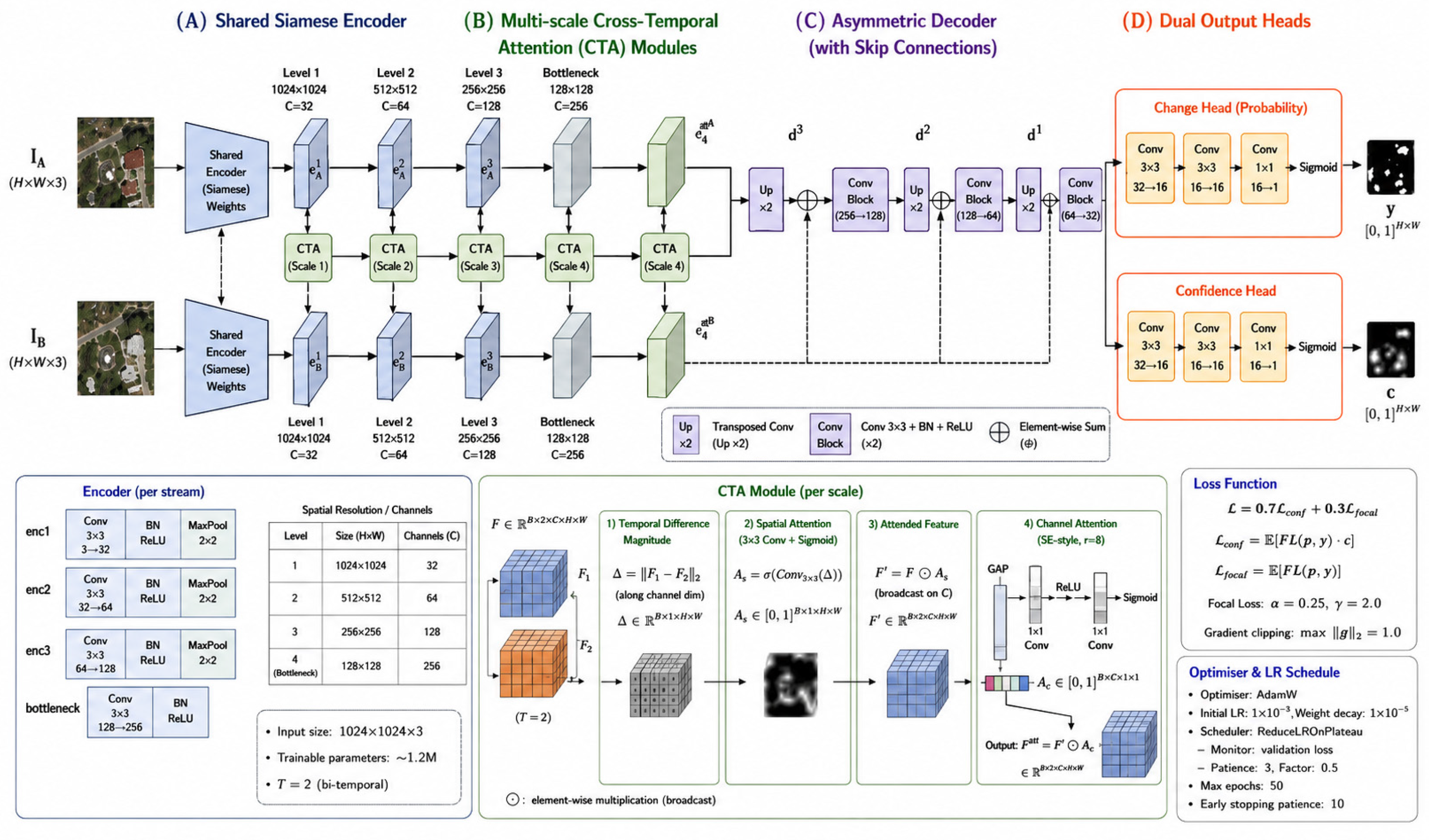
Figure 1. Proposed architecture.
Bdcc 10 00225 g001
Figure 2. Training and validation loss, IoU, and F1-score over 50 epochs on LEVIR-CD.
Bdcc 10 00225 g002
Figure 3. Comprehensive training history: individual curves (top), loss comparison, combined metrics, and overfitting indicator (bottom).
Bdcc 10 00225 g003
Figure 4. Pixel-level confusion matrix on the LEVIR-CD test set. Values represent total pixel counts.
Bdcc 10 00225 g004
Figure 5. ROC curve for the change class on the LEVIR-CD test set.
Bdcc 10 00225 g005
Figure 6. Precision–recall curve for the change class on the LEVIR-CD test set.
Bdcc 10 00225 g006
Figure 7. Qualitative change detection results on four LEVIR-CD test samples. Columns: (a) pre-change image, (b) post-change image, (c) ground truth mask, (d) CTA-Net prediction, (e) FC-Siam-conc prediction, (f) BIT prediction.
Bdcc 10 00225 g007
Figure 8. Multi-scale feature response visualizations.
Bdcc 10 00225 g008
Figure 9. Confidence analysis: (a) distribution of model confidence scores with inset showing detail near zero, (b) confidence versus prediction correctness, (c) calibration curve.
Bdcc 10 00225 g009
Table 1. LEVIR-CD dataset statistics.
SplitImage PairsTotal PixelsChange Ratio (%)
Training445467,697,600∼4.2%
Validation6467,108,864∼4.1%
Test128134,217,728∼4.2%
Table 2. Comprehensive performance metrics of CTA-Net on the LEVIR-CD test set.
MetricValue
Overall accuracy98.99%
Change precision90.67%
Change recall (sensitivity)84.87%
Change F1-score87.68%
Change IoU (Jaccard Index)78.06%
Specificity (TNR)99.62%
Cohen’s kappa (κ)0.8715
Matthews Correlation Coefficient (MCC)0.8721
False positive rate (FPR)0.38%
False negative rate (FNR)15.13%
Table 3. Comparison of CTA-Net with state-of-the-art methods on LEVIR-CD.
MethodAccuracy (%)Precision (%)Recall (%)F1 (%)
FC-Siam-conc [9]98.4991.9976.7783.69
SNUNet [25]98.8185.6090.1787.82
BIT [22]98.7589.2489.3789.31
ChangeFormer [36]98.8592.0588.8090.40
STANet [40]98.6683.8191.0087.26
USSFC-Net [20]98.8790.1290.1190.11
VcT [46]99.0192.5787.6590.04
HANet [47]99.0291.2189.3690.28
CTA-Net (Ours)98.9990.6784.8787.68
Table 4. Ablation study results on the LEVIR-CD test set.
VariantCTA ModulesConf. HeadF1 (%)IoU (%)Params
BaselineNoNo83.2171.240.91 M
+CTA onlyYesNo85.9475.311.10 M
+Conf. onlyNoYes84.6773.520.98 M
Full CTA-NetYesYes87.6878.061.2 M
Table 5. CTA-Net fine-tuned on Sentinel-2 agricultural imagery—test set metrics. All masks generated via NDVI-delta thresholding; see text for discussion of evaluation limitations.
MetricValue
Accuracy94.54%
Precision94.94%
Recall95.42%
F1-score95.18%
IoU90.81%
Disclaimer/Publisher’s Note: The statements, opinions and data contained in all publications are solely those of the individual author(s) and contributor(s) and not of MDPI and/or the editor(s). MDPI and/or the editor(s) disclaim responsibility for any injury to people or property resulting from any ideas, methods, instructions or products referred to in the content.