The Impact of Geometric Modifications and the Signal Plan Optimization of Intersections in an Urban Area

Abstract

The aim of this research is to analyze new proposals for the organization of traffic in the intersection model with rational solutions to increase its performance. The intersection represents a traffic node on a major European corridor and can be classified as highly loaded with frequent traffic jams. The signal-controlled intersection does not currently provide a suitable solution for traffic jams. Using Aimsun version 8 software, a detailed model of the intersection was developed, where the current situation and nine alternative scenarios (an optimization of the signal plan, an addition of a fourth signal phase, a widening of the connecting lane and the construction of an overpass) were tested. The simulation results were compared with the results of calculations according to the applicable technical regulations. The performance was evaluated based on delay time, travel time, queue length, and vehicle speed. The results showed that the overpass is the most effective solution, significantly reducing delay times and improving traffic flow. While other solutions offered local improvements, the overpass provided the most significant overall performance increase.

1. Introduction

Traffic flow theory represents a very wide research field. In mathematics and traffic engineering, traffic flow can be viewed as the observation of interactions between intersection users (pedestrians, cyclists, drivers, and their vehicles) and the infrastructure (highways and roads) with the intention to propose the effective and optimal traffic network with minimal traffic congestions [1].

The traffic light system is one of the most efficient ways to control the traffic flow [2]. The accurate estimation of its capacity is a very important role for traffic engineers for proper setting of the controlling of light-signal intersections. Green light duration as well as red light duration settings depend on the traffic density for the optimal and equitable length of the traffic queue and waiting time at the traffic light [3,4,5].

2. Literature Review

Speed, intensity, and density are basic characteristics of traffic flow, and their quantification is needed to understand real situations in traffic [6]. Relations between these three characteristics give a better representation of traffic flow; moreover, they help in planning, and in projects creating and in the operation of equipment on land roads [7]. Lighthill and Witham [8] as firsts made big progress in macroscopic traffic modelling. Richards [9] supplemented their work and laid the foundation of “macroscopic traffic flow modelling” [10].

Nowadays, when people want to travel more often and faster, the density of the traffic increases together with related problems. These problems are observable mainly in urban areas and the adjacent roads connected to them. Therefore, the current economy is increasingly dealing with the time spent in vehicles, which is directly related to traffic density. This is where modeling is very helpful [11].

Traffic models are fundamental for traffic simulations and play an important role in traffic research as well as in several traffic applications, like traffic flow prediction, car accident detection, or traffic management [12]. In [13] they proposed a model to estimate the probability that a vehicle will pass through an intersection within the signal phase. Based on the estimated probability, an optimal speed is generated and the vehicle (driver) is advised to either slow down (to avoid aggressive braking) at the red signal or accelerate (to pass through the intersection) at the green signal. In order to improve the operation of traffic lights and reduce the overall delay of traffic jams, in the paper [14] they proposed a software solution for the operation of the traffic light system that will enable an adaptive mode of operation at a traffic light-controlled intersection.

Traffic flow theory is elaborated including traffic modelling and simulation in [15]. The recent development in traffic flow modelling [16] represents an overview of the field of analysis and a modelling of the traffic flows. The purpose of the models is for planning and evaluating possible traffic disruption. The examples of specific issues [17] aimed at modelling and simulations, and studies related to them, are understanding the traffic function [18,19,20,21], the planning of new road infrastructure [22,23,24,25], and traffic management for traffic safety and controlled traffic lights [3,4,26,27].

Intersections used to be marked as limitations of the traffic network, meaning that the fluency of the traffic flow is becoming decelerated with the capacity exceeded. There is an estimate that the traffic signals delay contributes 5–10% to traffic delay in the whole world [28]. Microscopic models and simulations of traffic situations on intersections are necessary tools for the efficient planning and controlling of urban mobility [29], because of the need to improve quality of life and sustainable urban development [30]. In addition, microsimulations can be useful for traffic movement improvement, for example for traffic light controlling or possible construction modifications to the intersection.

The stop-and-go traffic flow method belongs to the basic options for controlling the traffic where traffic lights signaling equipment is used [31]. The intersection settings can be experimentally edited with the simulation of this method and then optimized in a real system [32,33,34]. Traffic fluency is one of the indicators of excellent intersection management, especially in traffic light settings at intersections [1,2,8].

With the intention of reducing the blocking traffic flow at traffic light-controlled intersections, the speed control strategy was used in [35]. Results show the reduction of the average time by at least 15% when vehicles are passing the intersection as well as the significant reduction of the delay of vehicles by 10–30% with various lengths of the signal plan.

Researchers from Shanghai [36] focused on green-light timing and red-light timing optimization using the simulation software VISSIM version 8. The efficiency of optimizing traffic control at the intersection indicated a reducing of the traffic overload. Many of the following studies [36,37,38,39] chose for the optimization of four basic parameters from signal plans (the length of the cycle, the green light duration, the sequence of phases, and the yellow time) for the minimization delay time or the length of the queue.

Also, authors in [33] realized the experiment with three traffic light intersections in Haifa (Israel) based on the simulations of 27 different scenarios’ optimized signalization plan with the aim to minimize average delays. The result of the experiment provided a reduction of the delays by 35% compared to plans implemented in the field.

The case study with data collected at Foothill Blvd in Los Angeles [40] demonstrates that a new signal plan proposal is beneficial at more than 90% of the 408 analyzed cycles. The analysis also showed that the average improvement of the green light duration is significant for synchronized phases.

Harahap et al. [41] used program MATLAB version R2015b for the optimal traffic lights setting depending on waiting time reduction. Firstly, the average speed of vehicles incoming to an intersection then the average delay time were estimated. Based on selected parameters, the delay time was reduced from 130 s to 55 s.

There are many alternatives for editing the flow of vehicles and the geometry of the infrastructure. In the following study [42], they compiled an overview of three alternatives: light-signal control, a turbo roundabout, and a road overpass. The verification of those alternatives showed that the installation of traffic lights signalization influenced the current situation by reducing the incoming speed by 38%, though a permanent solution for traffic performance requires the road overpass which can increase the traffic speed four times.

Bakhsh [43] compared the current situation with two alternatives. The analysis showed that roundabouts with lights signals achieved the lowest traffic performance, in other words, a prolonged delay time. The alternative without roundabouts appeared the most appropriate.

Another study [44] aimed at increasing traffic performance in Palembang (Indonesia) using several alternatives. The microsimulation software VISSIM 8 was used. The results of the analysis and the modeling performed showed that the best solution to optimize the traffic performance of chosen intersections is geometric edits and traffic diversion at the intersection. The delay time reduction can be 62% and 45%, respectively.

Especially in the scenario with road overpass construction, geometric edits at intersections and signal plan optimization was most appropriate. The exhaust emissions were reduced by 32.36%, resulting from the length of the queue being reduced by 44% and the delay time by 57.05% in this alternative [45].

A considerable group of factors has an influence on the simulation or modelling of the traffic flow at intersections in all of the mentioned studies and their analyses. For example, drivers in the USA spend 97 h in traffic because of traffic overload which is equal to annual time costs of 87 billion dollars [46]. Travel time is one of the highest categories of the traffic costs and time saving is considered as the most important benefit in traffic projects, like land roads and public transportation improvements [47]. For this reason, studies of the impact of delays at intersections are important.

Simulations are the way to verify various scenarios, so that we can then compare or evaluate the advantages of each variant. It is necessary to consider the right characteristics for the simulating in software, like the acceleration or deceleration of the vehicles. The construction edits of intersections have influence on the delay time reduction. The improvements reflect also the emissions or traffic noise reduction. Models can be helpful for predicting, estimating the impact of various interventions in systems, and better planning the required actions.

3. Materials and Methods

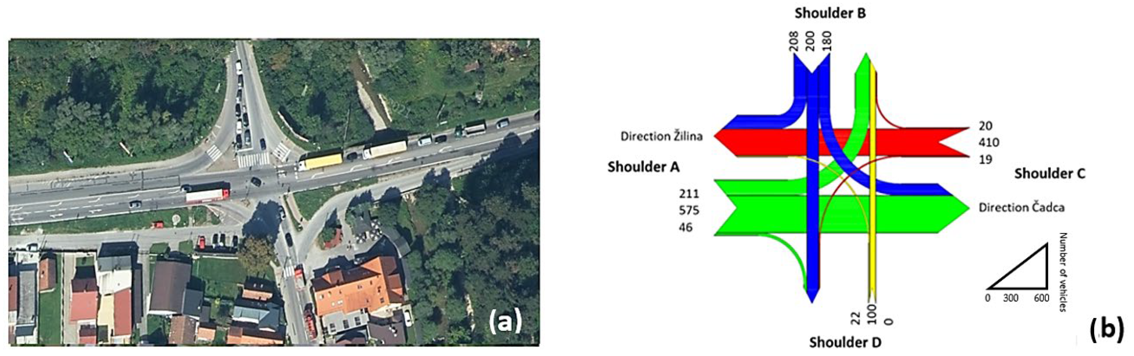
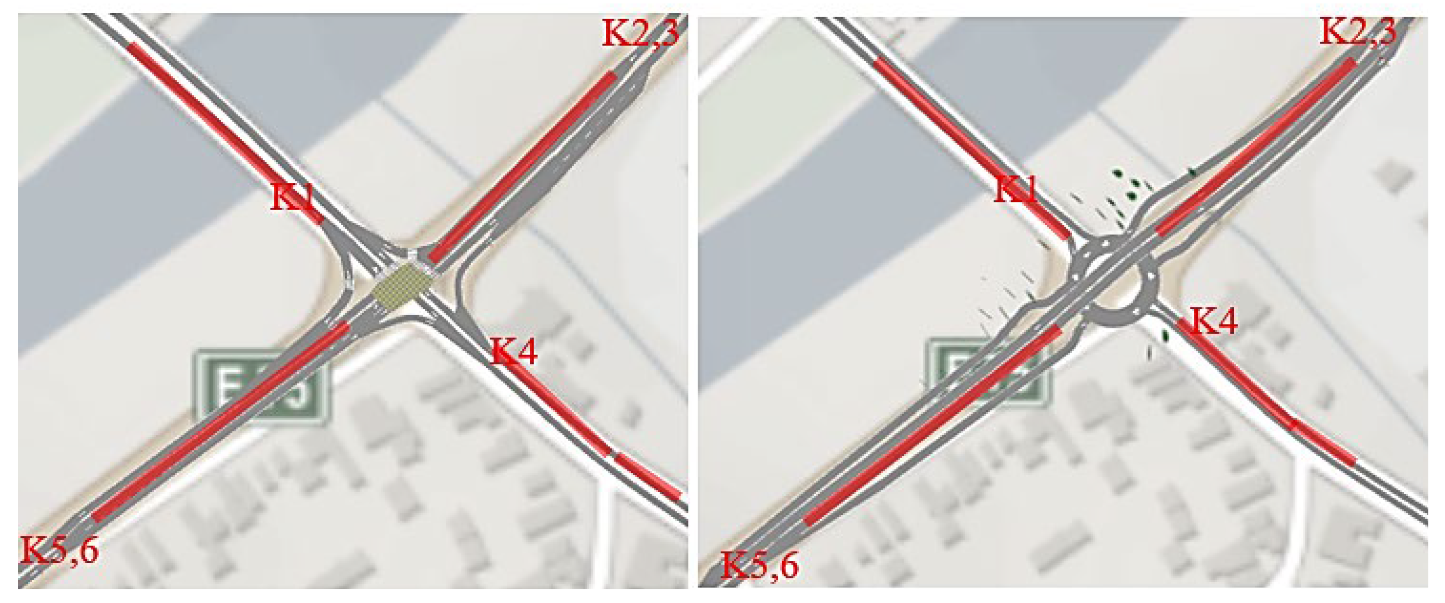
As mentioned above, the aim of this study is to analyze traffic issues on selected intersections by simulations of various scenarios. All of the scenarios were proposed based on other available studies and then tested by simulation in Aimsun version 8 software. The simulating model was created based on the data collected during the traffic survey oriented on the characteristics influencing traffic fluency. The observed intersection for this research is placed in the urban area of the town of Kysucké Nové Mesto, where also leads the European road nr. E75 (Figure 1a).

Over the last five years, traffic volume has increased by a total of 10%. Truck traffic passing through the selected intersection makes up approximately 40%, while their increase was 8% from 2020 to the present. The proportion of vehicles was 3% higher over the same period [48]. The input data needed for the simulation were collected during the traffic survey presented in this research. The vehicle intensity was stated to be more than 2000 vehicles per hour. The traffic overload is visible in Figure 1b.

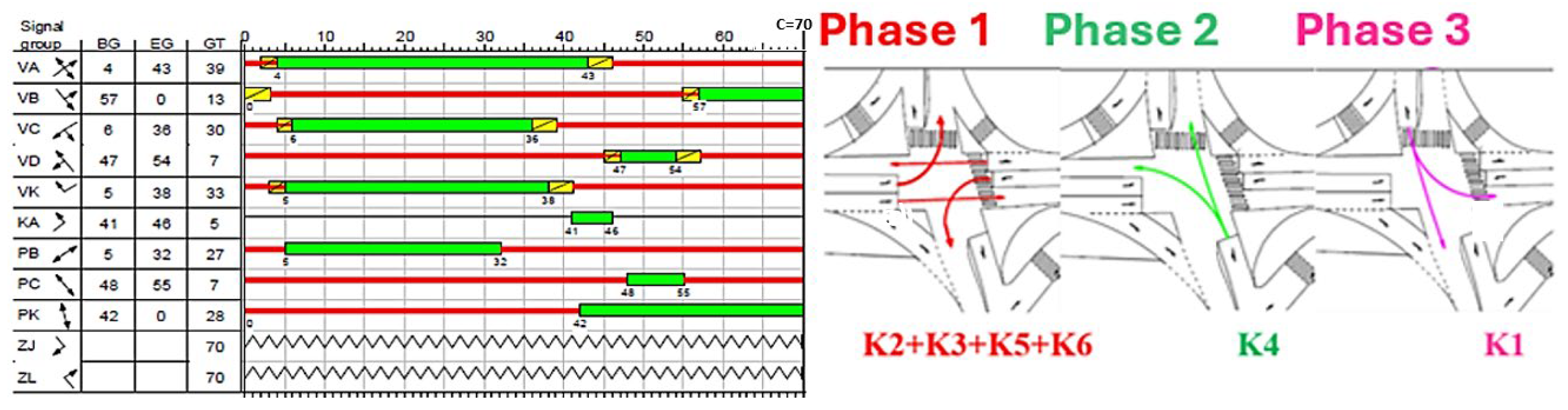
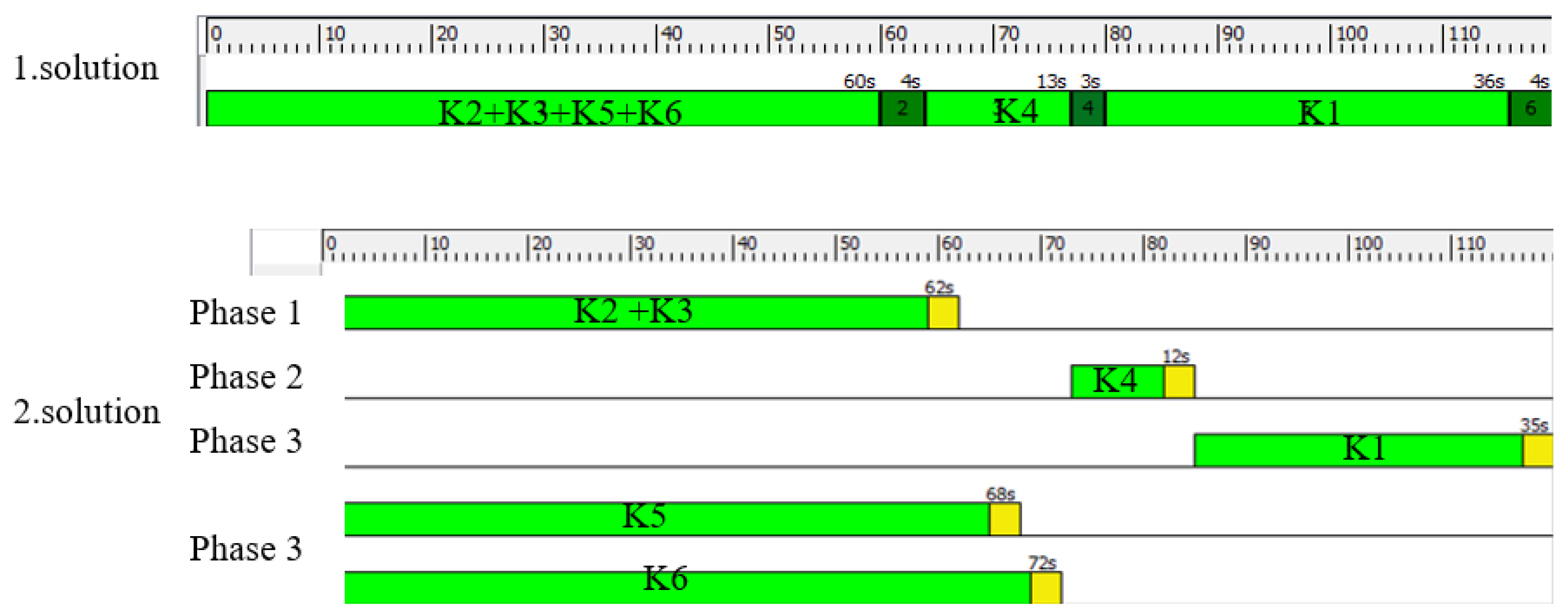
The selected intersection can be classified as lights-signal controlled and the intersection signal plan with the phases order is in Figure 2.

The length of the cycle is determined at 70 s. In the first phase, groups VA, VC, KA, and VK heading from shoulder A and shoulder C, i.e., direction K2, K3, K5, and K6, can pass through the intersection. KA is an extension of green by 3 s in direction K6. Subsequently, the second phase VD from shoulder D has a green light on, i.e., direction K4. In the last phase, for group VB, turning vehicles are heading from shoulder B and thus in direction K1. The other groups PB, PC, and PK are green for pedestrians.

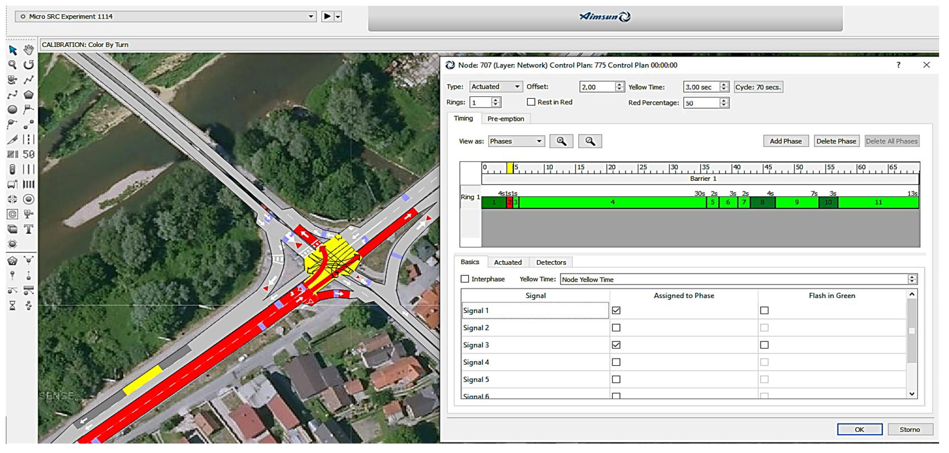
The detailed intersection model was created by Aimsun version 8 software including geometric parameters, traffic flows, and the intersection signal plan (Figure 3). The intersection is in the simulation model created as the fixed time light-signal control intersection, also known as offline control, what means that the signal timing is predetermined [49].

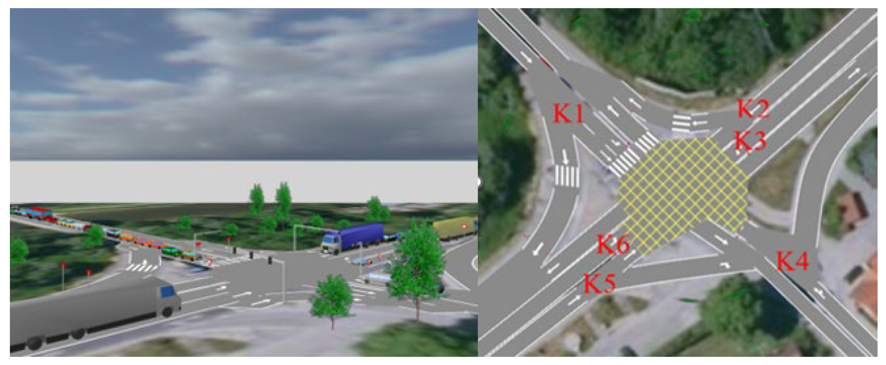
Traffic intensity data collected during the mentioned survey were used for creating the simulating model of the intersection. Vehicles participating in the model were divided into four categories: cars, trucks, heavy trucks, and public transport (buses). The simulation duration was stated at 1 h and together 83 simulations for each variant (current situation and new proposals) were realized. 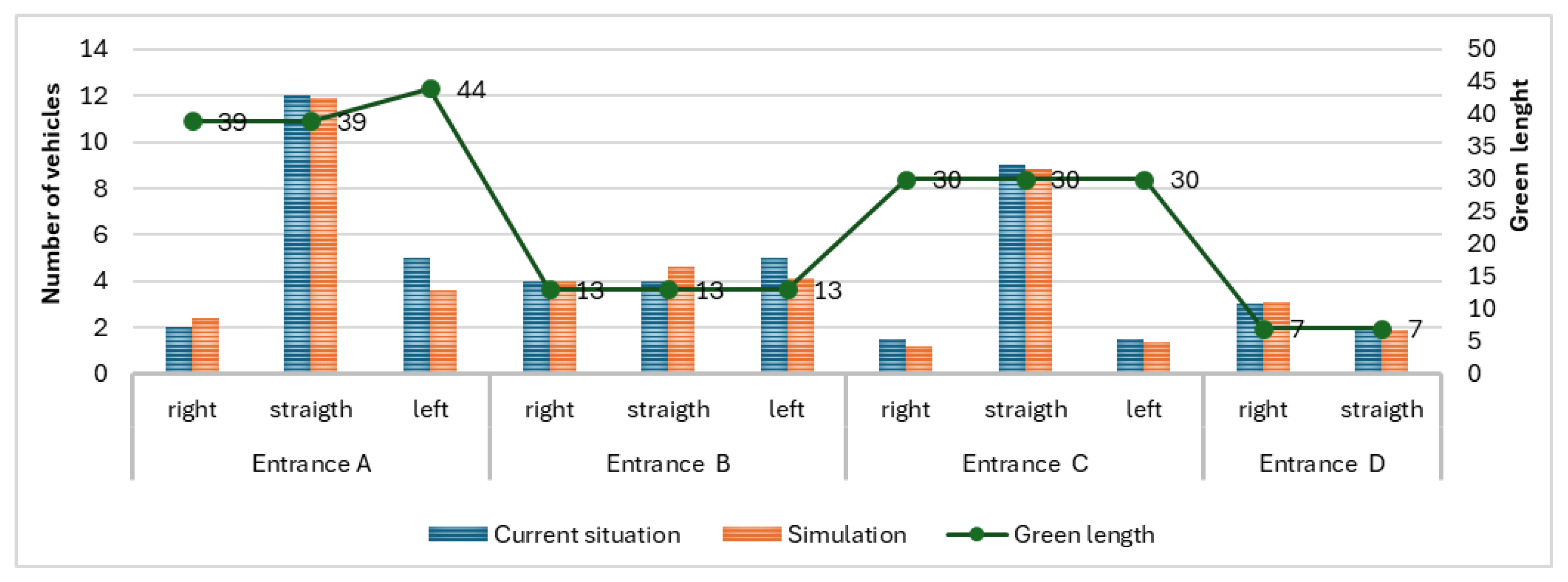The formula given in [50] was used to determine the required number of simulations and calibration. The observed indicators were expressed as mean values from repeating simulations. The simulation process and the labelling of the individual directions are shown in Figure 4.

The Aimsun version 8 software processed various variants of the intersection solutions and followed the comparison of individual solutions. The whole outputs of the simulation’s observed indicators were compared for the current situation, signal plan optimization, new phases proposal, and geometric edits at intersection. New proposals were made every time compared with the current situation. Several outputs were evaluated, like travel time, delay time, and the length of the queue. Based on previous research, we formulated some research questions.

Do the optimized signal plans, derived through different methods, result in a significant improvement in the quality of service at the intersection compared to the existing signal plan? Which geometric modification, lane extension, or overpass construction offers the greater benefit in terms of reducing delay and queue length?

Which of the proposed solutions (signal plan optimization, new phase introduction, or geometric modifications) offers the most significant improvement in overall traffic performance at the intersection?

How do the various solutions compare in terms of their impact on different traffic characteristics (delay time, travel time, queue length, and vehicle speed) for each direction?

4. Results

4.1. Simulation of the Current Situation at the Intersection

The aim of the analysis was to analyze the current relations and conditions at the intersection. The average values of delay time, travel time, the length of queues, and the speed of vehicles were the observed indicators as simulation outputs in individual directions K1–K6.

Direction K1 has the longest delay time and the lowest speed. It seems that there are the biggest problems with traffic fluency in this direction. The traffic queue can be about 500 m long and then interfere with downtown traffic. Direction K4 has the shortest delay time and the highest speed of vehicles, which makes the traffic situation the most favorable in this direction (

Table 1. Average values of the chosen indicators as a simulation output in individual directions.

Direction	Delay Time [s]	Travel Time [s]	Queue [veh]	Speed [km/h]
K1	113.2	121.8	25.4	4.8
K2	34.1	42.2	10.9	16.1
K3	67.4	59.1	1.7	10.5
K4	9.4	15.8	1.7	44.1
K5	21.1	28.2	11.5	19.4
K6	72.2	79.9	11.1	10.9

).

There are very significant differences in the length of the queues between all directions. Traffic intensity, green light duration, or the geometric configuration of the intersection can represent factors that cause these differences.

The most important measured value for evaluating the quality of traffic fluency (QSV) at the light-signal-controlled intersection shoulder is the wait time. The quality level of the intersection was evaluated in accordance with the Technical Conditions 102 (TP 102) as the national norm for Slovak republic. The evaluation was based on the delay time at the entrances. All criteria for the evaluation are listed as indicators in

Table 2. Average waiting time thresholds for determining the quality level.

Quality Level (QSV)	Average Delay Time [s]
A	≤20
B	≤35
C	≤50
D	≤70
E	≤100
F	>100

.

Characteristics of the traffic quality level:

Level A: Most traffic participants can pass the intersection without restrictions. The delay time is very short.

Level B: All traffic participants arriving during a red light can continue driving during the following green light. The delay time is short.

Level C: Most traffic participants arriving during a red light can continue driving during the following green light. The delay time is noticeable.

Level D: Vehicles constantly form a remaining queue. The delay time of all the traffic participants is considerable.

Level E: The traffic situation is unstable; even small changes in traffic load will cause a sharp increase in time losses. The delay time is long.

Level F: The intensity is greater than capacity. The delay time is very long. The intersection is congested.

In motor vehicle traffic, (AWT) includes the total time loss that must be taken into account in the case of continuous vehicle movement. The wait tie contains two main parts [51]:

• The basic wait time that represents the waiting time during the red lights duration;
• The delay time of the remaining queue, which occurs with vehicles who fail to leave when during the green light, restricting the following vehicles (delay time).

The following

Table 3. Quality comparison of the traffic flow at the intersection in individual directions.

Direction	Calculation According to TP 102		Simulation
	Delay Time [s]	QSV	Delay Time [s]	QSV
K1	1561.69	F	113.2	F
K2	34.16	B	34.1	B
K3	11.53	A	67.4	D
K4	44.48	C	9.4	A
K5	26.17	B	21.1	B
K6	516.41	F	72.2	E
Final QSV		F		F

compares values of the delay time from the simulation with values obtained by calculation based on TP 102.

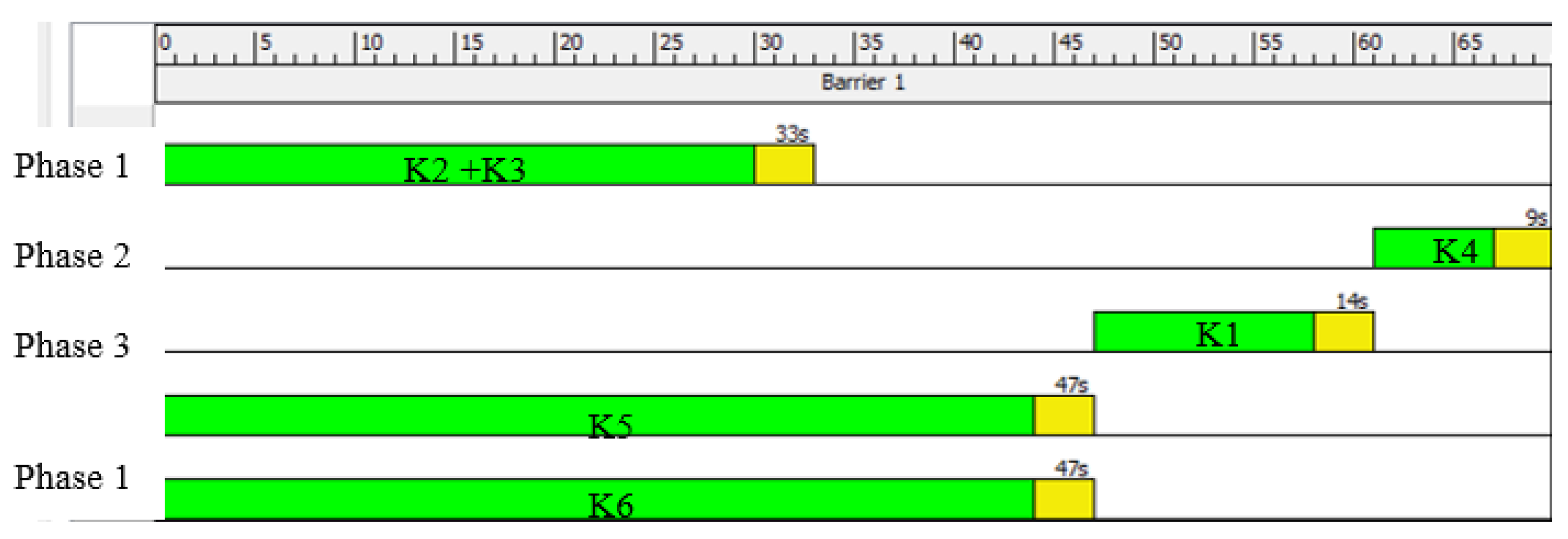
4.2. Variant I—Signal Plan Optimization

The signal plan optimization consisted of several alternative solutions (I.A, I.B, and I.C). Firstly, the lengths of the signal plan were changing based on the calculations from TP102 with regard to current conditions. Next, the generation of the new signal plan in the Aimsun version 8 software was processed and finally a mathematical model for optimization was used.

4.2.1. The Change of the Length of the Signal Plan: Alternative I.A

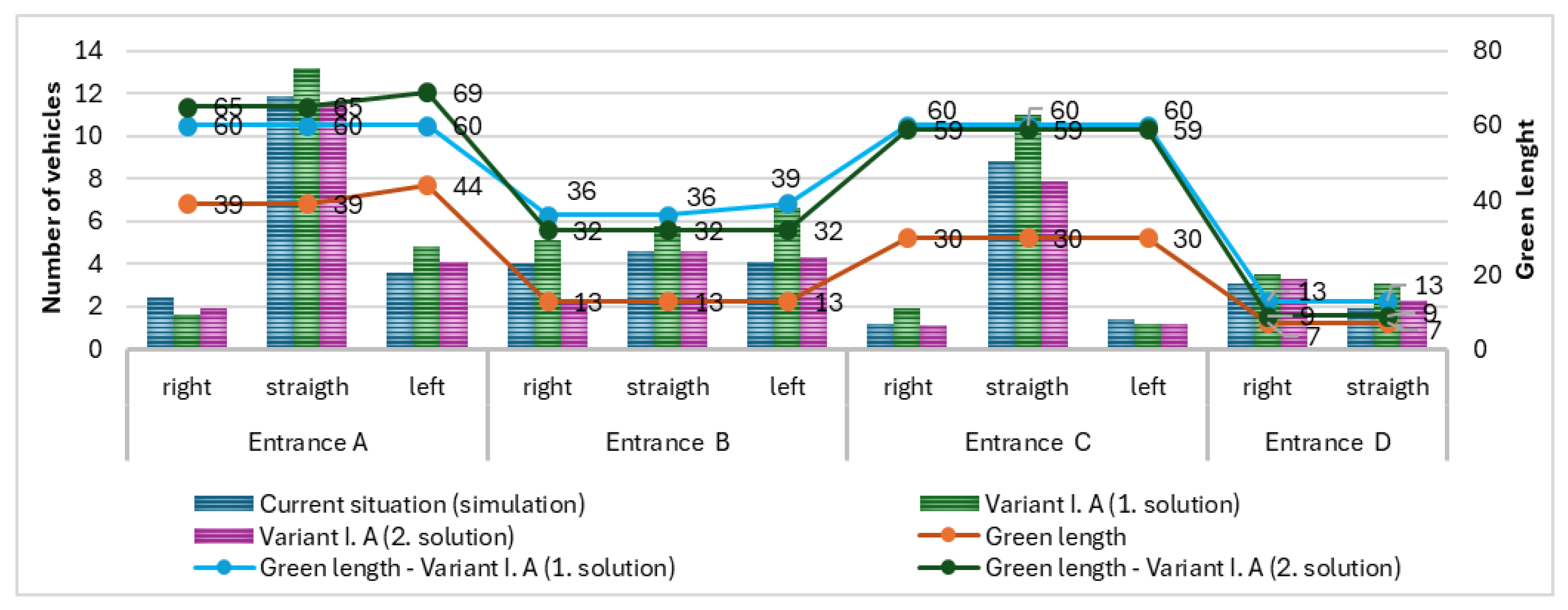
The optimization of the current situation at the intersection based on the TP102 and input data from the survey marked out the cycle duration at 120 s. In the first solution, the green light duration was stated equally on 60 s for directions K2, K3, K5, and K6, and on 13 s for direction K1. In the second solution, the logic changes regarding current light signalization control were applied as follows: various combinations of different green light duration settings while maintaining three cycles. For directions K2, K3, K5, and K6 different lengths of 59 s, 65 s, and 69 s were stated in the same order. Then, 9 s was the time stated for the direction K4, and the green light duration in the K1 direction was 32 s. Yellow times remained in the original length of 4 s, 3 s, and 4 s again (Figure 5).

The resulting values for individual directions as an output of the simulation are described in the following

Table 4. Simulation output values for two solutions.

Direction	1. Solution				2. Solution
	Delay Time [s]	Travel Time [s]	Queue [veh]	Vehicle Speed [km/h]	Delay Time [s]	Travel Time [s]	Queue [veh]	Vehicle Speed [km/h]
K1	24.0	32.7	14.2	28.9	46.7	55.4	6.4	21.4
K2	21.5	29.5	4.8	25.7	64.3	72.3	6.3	6.9
K3	40.7	48.9	1.4	16.1	176.2	184.5	2.4	4.3
K4	19.6	26.2	2.8	38.1	11.5	18.0	1.7	43.6
K5	31.7	38.6	12.3	20.8	36.9	42.9	13.1	10.5
K6	223.5	231.2	18.7	3.3	96.9	104.4	12.8	7.0

:

The highest delay time of 223.5 s appeared in the first solution for the K6 direction. This resulted from the fact that the speed of the vehicles in this lane was the lowest (3.3 km/h) and the length of the queue was the longest. In the second solution, the delay time decreased, but it increased in the K3 direction to 176.2 s. This implies that the worst traffic conditions were in the left-turn lane from the main road in both solutions.

The following

Table 5. The quality level comparison for two solutions in I.A variant optimization.

Direction	1. Solution				2. Solution
	Simulation		Calculation According to TP 102		Simulation		Calculation According to TP 102
	Delay Time [s]	QSV	Delay Time [s]	QSV	Delay Time [s]	QSV	Delay Time [s]	QSV
K1	24.0	A	52.98	D	46.7	C	52.36	D
K2	21.5	A	27.90	B	64.3	D	28.03	B
K3	40.7	C	15.15	A	176.2	F	15.63	A
K4	19.6	A	51.32	D	11.5	A	66.98	D
K5	31.7	B	48.76	C	36.9	C	37.01	C
K6	223.5	F	17.14	A	96.9	E	12.38	A
Final QSV		F		D		F		D

represents a comparison of the quality level of both solutions between the capacity evaluation and simulation:

The determined delay time achieved minimal deviations through the capacity evaluation, except K4 and K5 directions (Table 4). These deviations had no influence on the quality level, and the QSV was rated at level D in both cases. The traffic quality was rated at level F based on the simulation. In the first solution, three directions K1, K2, and K4 reached quality level A, while only the K4 direction was rated with level A in the second solution.

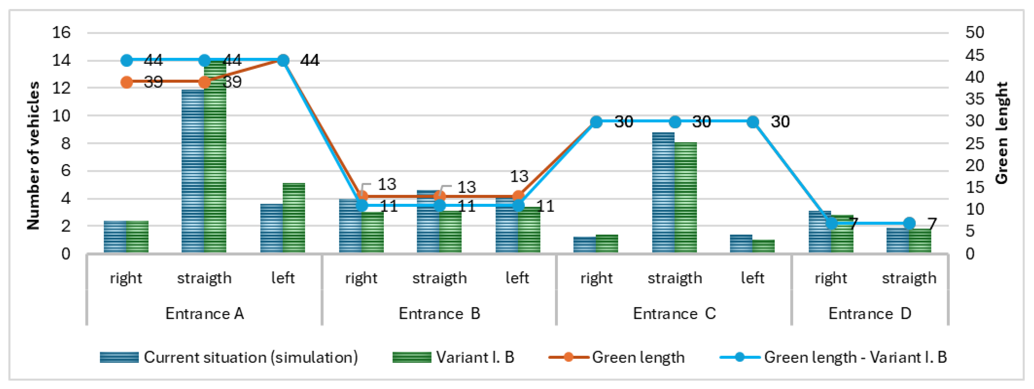
4.2.2. The Generation of the Signal Plan in Aimsun Software—Alternative I.B

The Aimsun version 8 software offers the possibility to generate a new control plan from volumes with options of fixed or dynamic signal plans. This option was realized as a solution for the current situation optimization (Figure 6). Conditions needed as entering criteria were, for example, the minimal green light duration (5 s) and traffic intensity in individual directions. The intervals of cycle lengths were chosen between 70 and 100 s.

In this solution, the highest delay time was observed in the K1 direction (113.9 s) with quality level F. This implies the lowest speed of vehicles and the longest traffic queue. The best results and most appropriate values were observed in the K5 direction.

As can be seen in

Table 6. Simulation output values for individual directions.

Direction	Delay Time [s]	Travel Time [s]	Queue [veh]	Vehicle Speed [km/h]
K1	113.9	118.6	24.7	7.1
K2	17.7	25.7	4.2	25.4
K3	35.3	43.4	1.4	15.8
K4	37.8	44.2	3.4	36.4
K5	9.2	16.2	8.8	31.7
K6	26.8	34.5	6.9	19.5

, the K1 direction determined the worst values. The traffic quality reaches the worst level in both comparisons which is reflected in the total quality level of the intersection. The resulting quality level is rated as F (

Table 7. A quality level comparison of the generated signal plan.

Direction	Calculation According to TP 102		Simulation
	Delay Time [s]	QSV	Delay Time [s]	QSV
K1	113.9	F	2525	F
K2	17.7	A	54.30	D
K3	35.3	C	11.53	A
K4	37.8	C	180.25	F
K5	9.2	A	16.35	A
K6	26.8	B	5.50	A
Final QSV		F		F

).

4.2.3. Light Signal Duration Optimization Based on a Mathematical Model: Alternative I.C

The process explained and used in [52] was applied for the following calculation. The initial assumptions are formulated as follows: the occurrence of vehicles has a Poisson distribution and the probability distribution of the time until the next variable occurs is exponential with parameter λ based on the Equation (1).

$$\mathrm{P}\left(\mathrm{N}=\mathrm{x}\right)={\displaystyle \frac{{\mathsf{\lambda }}^{\mathrm{x}}}{\mathrm{x}!}}{\mathrm{e}}^{-\mathsf{\lambda }}$$

(1)

The sum of the green light duration was stated as 59 s and parameters λi were determined based on the number of vehicles passing through the intersection during the green light in the selected direction. The conditions were established using nonlinear programming in MS Excel (MS 365). Then, the optimal green light duration was sought for in three concepts:

(a)

The sum of the mean values of the waiting time for the green light was minimal;

(b)

The sum of the mean values of the waiting time was minimal and the sum of the mean values of the total unused green light time was minimal;

(c)

The maximal value from the mean vehicles’ waiting time for the green light and the sum of the mean values of the total unused green light time was minimal.

The duration of the green light was optimized using MS Excel Solver, considering the established concepts (

Table 8. The resulting values of the optimized green light duration in individual directions using the mathematical model.

Concept	x1 [s]	x2 [s]	x3 [s]
a	39.76 (40)	14.23 (14)	5
b	38.91 (39)	15.09 (15)	5
c	24.95 (25)	19.1 (19)	14.95 (15)

).

All of the mentioned values were changed in the simulation settings and tested. The results are processed in the following

Table 9. The simulation output resulting values of the optimization using the mathematical model.

Direction		K1	K2	K3	K4	K5	K6
Concept a	Delay time [s]	72.4	10.4	32.6	334.7	19.4	106.5
	Travel time [s]	81.1	18.4	41.5	343.1	26.4	114.4
	Queue [veh]	20.6	3.4	1.4	12.8	11.3	14.0
	Vehicle speed [km/h]	13.1	32.2	16.9	13.2	20.6	7.4
Concept b	Delay time [s]	51.1	10.8	33.5	531.1	23.5	134.1
	Travel time [s]	59.8	18.9	41.8	537.2	30.5	147.3
	Queue [veh]	17.3	3.5	1.4	16.2	12.1	16.8
	Vehicle speed [km/h]	19.8	31.7	16.2	2.5	17.5	5.8
Concept c	Delay time [s]	13.5	75.2	40.4	1.5	24.5	1800
	Travel time [s]	22.3	83.8	31.8	7.7	41.9	1800
	Queue [veh]	9.6	6.3	1.4	0.6	19.9	19.5
	Vehicle speed [km/h]	36.7	5.3	12.1	48.1	2.4	0.27

:

As can be seen, the observed values were changing for each individual direction (K1–K6) and in every concept of the traffic lights signal settings. However, the highest vehicle speed was achieved in the first concept a, where the sum of the mean values of the waiting time for the green light turned on were minimal (similar to the current situation). On the contrary, the least effective result was given using the concept c, where the maximal value from the mean vehicles’ waiting time for the green light turned on and the sum of the mean values of the total unused green light time was minimal. In this way of optimization (concept c), the K6 direction (turning left from the main road) achieved a waiting time of more than 1800 s and the vehicle speed was almost 0 km/h. The reason for the high waiting time mentioned is the extension of the green time in phase 3 (x₃).

Data from

Table 10. A quality level comparison using the mathematical model.

Direction	Concept a				Concept b				Concept c
	Simulation		Calculation According to TP 102		Simulation		Calculation According to TP 102		Simulation		Calculation According to TP 102
	Delay Time [s]	QSV	Delay Time [s]	QSV	Delay Time [s]	QSV	Delay Time [s]	QSV	Delay Time [s]	QSV	Delay Time [s]	QSV
K1	72.4	E	1191.38	F	51.1	D	880.33	F	13.5	A	29.06	B
K2	10.4	A	10.04	A	10.8	A	10.70	A	75.2	E	195.17	F
K3	32.6	B	6.51	A	33.5	B	6.94	A	40.4	C	14.62	A
K4	334.7	F	66.61	D	531.1	F	66.61	D	1.5	A	23.24	B
K5	19.4	A	23.76	B	23.6	B	26.17	B	24.5	B	342.36	F
K6	106.5	F	7.36	A	134.1	F	7.85	A	1800	F	16.53	A
Final QSV		F		F		F		F		F		F

imply that the comparison of all three concepts and the current traffic quality evaluation brings again level F. Directions K4 and K6 are becoming the most problematic in simulation concepts (a) and (b). Direction K6 is the most problematic again in simulation concept c. Some directions achieve appropriate similar delay time values for the simulation as well as for the TP102 calculation, for example, the K2 direction. Ultimately, the resulting quality level of the intersection for all of the concepts is rated with the worst level, F.

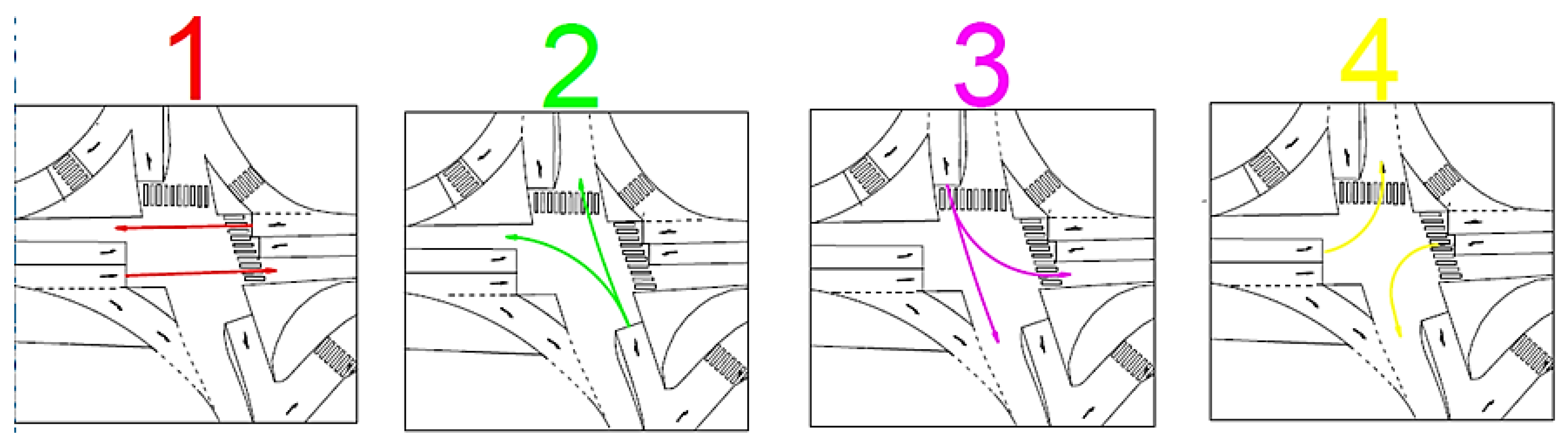
4.3. Variant II—The Introduction of New Phase (Phase 4)

A four-phase control of the intersection instead of a three-phase system is another proposed variant for improving the traffic flow. A separate phase should be introduced for left-turn vehicles with an intensity of more than 180 vehicles/hour according to TP102. The intensity of vehicles turning left from shoulder A was 241 vehicles/hour, and so the fourth phase was introduced as the next variety solution (Figure 7).

There are K2 and K5 directions included in phase 1, then the K4 direction is included in phase 2, the K1 direction is included in phase 3, and directions K3 and K6 are included in newly proposed phase 4.

Firstly, lengths of the lanes of the departing and arriving vehicles were measured, and then the yellow time duration between the individual phases was established. In total, 24 combinations of phases were realized. According to that, the yellow light duration was optimized considering the yellow light duration as lost time. The aim was to find the combination of phases with the minimal sum of the waiting time between green lights. In the results, there were four appropriate combinations, but the chosen one was a sequence of phases 1-4-2-3 with sums of the yellow light duration as 12 s.

Similar to the previous variants, the changes resulting from this solution were set in the software. Based on the simulations, their average data were exported for processing results (

Table 11. The simulation output of the four-phases control resulting values for individual directions.

Direction	Delay Time [s]	Travel Time [s]	Queue [veh]	Vehicle Speed [km/h]
K1	42.1	50.8	17.6	21.6
K2	26.0	34.1	10.8	22.7
K3	45.3	53.6	1.6	15.9
K4	241.7	271.4	11.1	13.6
K5	31.7	38.7	12.1	19.4
K6	237.2	245.3	18.8	2.9

).

The longest delay times were noticed for K4 and K6 directions. The introduction of a new phase was needed just because of the K6 direction. In this point of view, we can conclude that the introduction of a fourth phase is not efficient. The reduction of delay times was expected. The following

Table 12. A comparison of the quality levels in the four-phase control.

Direction	Calculation According to TP 102		Simulation
	Delay Time [s]	Delay Time [s]	Delay Time [s]	Delay Time [s]
K1	42.1	C	240.27	F
K2	26.0	B	39.24	C
K3	45.3	C	46.40	C
K4	241.7	F	240.14	F
K5	31.7	B	194.70	F
K6	237.2	F	105.65	F
Final QV		F		F

also shows these facts.

The evaluation of the delay time for the intersection is stated in the F quality level, as even the values of the delay time are lower for the simulation. The best traffic quality level is marked with B and the intersection capacity evaluation achieved the quality C level. Based on this evaluation, variant II represents the worst proposal for the improvement of the intersection.

4.4. Variant III—Addition or Extension Connection Lane

The following solution of the current situation is aimed at the geometrical editing of the intersection. The proposal of this solution was influenced also by studies [46,48], which elaborated on the research about similar problematics.

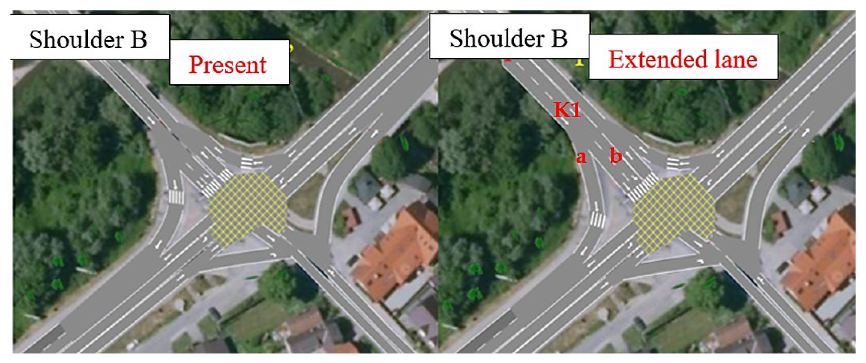
Especially the traffic lane on shoulder B from Kysucké Nové Mesto required geometrical editing. Currently, vehicles line up in one lane before the intersection for all directions (left, straight, and right) (Figure 8). The (almost) everyday traffic queue used to reach downtown throughout the whole day. The length of the queue was established at 25 m, which corresponds to approximately four units of vehicles. The survey showed that the direction from shoulder B is the most used during the peak hour. Vehicles driving from the K1 direction straight or turning left used to inhibit vehicles who were turning right. At the part of the shoulder that leads by the bridge, the successful editing of road lanes can help to relieve the load on it from the vehicles waiting in the queue.

Figure 8. The current situation and new proposal at the intersection. After the edits in the current signal plan in Aimsun version 8 software, the following results were processed (Table 13).

Figure 8. The current situation and new proposal at the intersection. After the edits in the current signal plan in Aimsun version 8 software, the following results were processed (Table 13).

Table 13. The resulting values for individual directions in variant III.

Direction	Delay Time [s]	Travel Time [s]	Queue [veh]	Vehicle Speed [km/h]
K1a,b	3.37	11.7	1.2	37.9
K2	24.2	32.2	9.0	20.1
K3	39.8	48.2	1.5	13.2
K4	0.8	7.2	0.3	49.9
K5	19.2	26.2	12.0	20.9
K6	66.3	74.1	11.4	11.3

Table 13. The resulting values for individual directions in variant III.

Direction	Delay Time [s]	Travel Time [s]	Queue [veh]	Vehicle Speed [km/h]
K1a,b	3.37	11.7	1.2	37.9
K2	24.2	32.2	9.0	20.1
K3	39.8	48.2	1.5	13.2
K4	0.8	7.2	0.3	49.9
K5	19.2	26.2	12.0	20.9
K6	66.3	74.1	11.4	11.3

The attention was focused mainly on the K1 direction, where the delay time reached the lowest value so far of 3.37 s. Also, the length of the queue was reduced and the average speed increased. The delay time for the K1 direction was calculated as a weighted average, where the weight was the vehicle intensity. The original values resulting from the simulation are presented in

Table 14. The observed quality levels in the variant.

Direction	Calculation According to TP 102		Simulation
	Delay Time [s]	QSV	Delay Time [s]	QSV
K1a	10.1	A	25.64	B
K1b	0.2	A	0.00	A
K2	24.2	B	10.70	A
K3	39.8	C	6.94	A
K4	0.8	A	44.48	C
K5	19.2	A	5.50	A
K6	66.3	D	133.64	F
Final QSV		D		F

.

The extension of the road lane placed right in shoulder B manifested as positive in the simulation. On the first try, the traffic quality level was marked as D. However, in the evaluation of the traffic quality based on the TP102 calculation, it reached level F at this intersection.

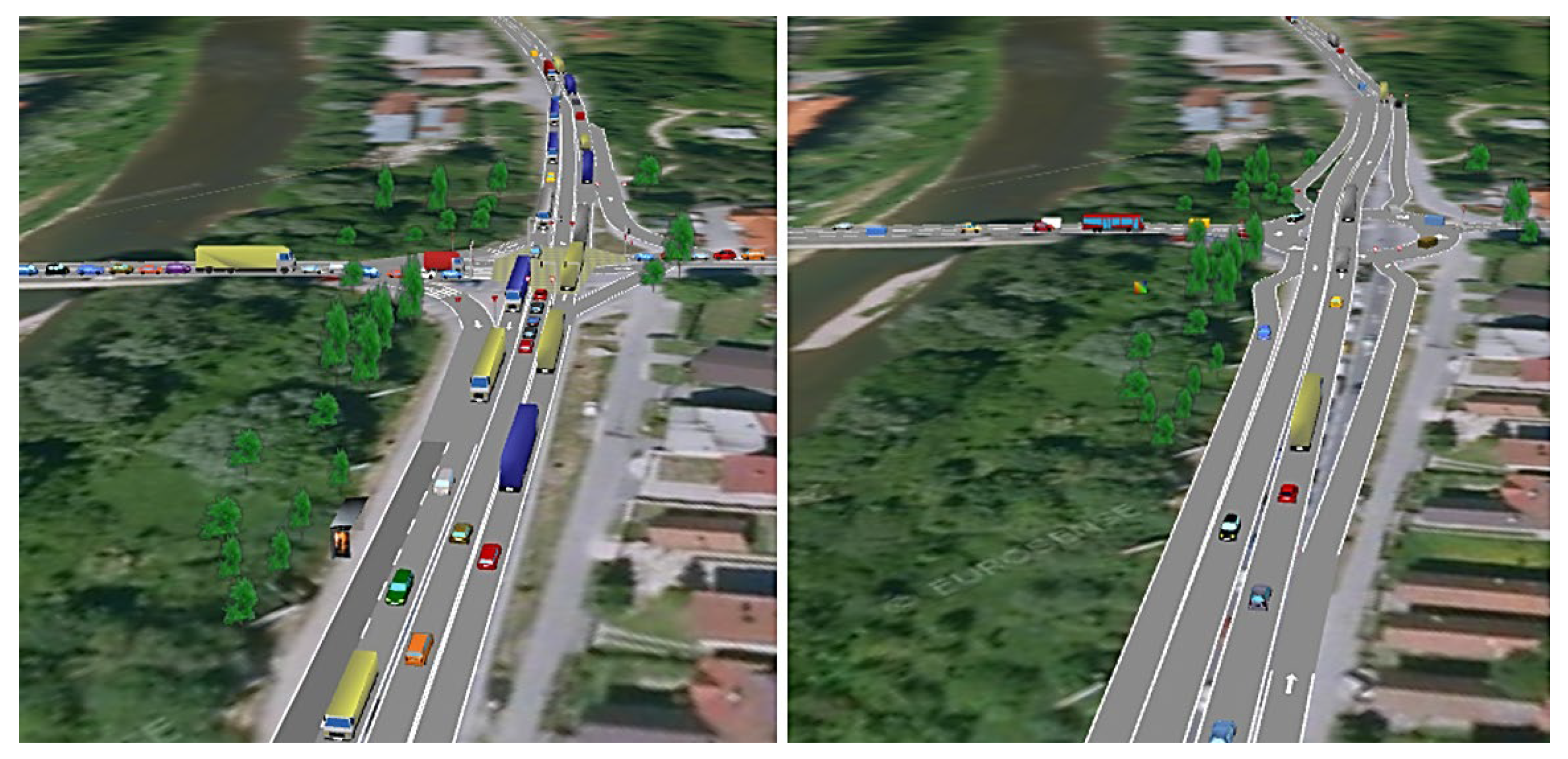
4.5. Variant IV—Overpass the Main Road

The last proposal for the solution to the current situation is bridging the main direction at the road nr. I/11. It is the main traffic flow of vehicles transiting in the direction from Žilina to Čadca and vice versa (shoulders A, and C and directions K2 and K5). An overpass will be added in the main direction, the main transit will be diverted, and the intersection could be transformed into a roundabout. Thus, a multi-level intersection would be created here because problems originate from the vehicles entering on the main road nr. I/11 from shoulder B. The bridge itself would start approximately 250 m before the border of the intersection, and in the same conditions, it would end (Figure 9).

The simulation of the current situation and proposed solution is shown in Figure 9, where the forming traffic queues are visible on the left while the proposed solutions visualize fluent traffic on the right.

The simulation was created with the intention to reflect the real traffic intensity at the intersection. Merging lanes that are long enough are the part of the proposal solution (more than 70 m) which should ensure that vehicles can fluently merge with the road I/11 from Kysucké Nové Mesto without any problems [53]. The visualization of proposed solution of Variant IV is on Figure 10 below.

The traffic light-controlled intersection was replaced by a roundabout with four shoulders. The overpass leads above this roundabout in the main road direction. The shoulders of the roundabout are connecting to an overpass at a distance of more than 70 m. The roundabout has only one driving lane with a width of 7.5 m. Also, the direction labelling changed from 6 to 4 (directions K2 and K3 as well as K5 and K6 were connected). The evaluation of the traffic quality was observed in the marked section of the intersection (Figure 10).

New parameters were set at the simulations and the outputs from their average are stated below.

Table 15. The resulting values for individual directions in the bridging of the main road variant.

Direction	Delay Time [s]		Travel Time [s]		Queue [veh]		Vehicle Speed [km/h]
	O	CS	O	CS	O	CS	O	CS
K1	3.6	113.2	13.5	121.8	2.6	25.4	40.3	4.8
K2,3	0.3	21.8	5.8	40.5	0	3.6	51.7	15.7
K4	6.8	9.4	11.8	15.8	3.5	1.7	33.12	44.1
K5,6	0.5	35.1	9.5	43.2	0	5.5	50.6	48.8

O—overpass, CS—current status.

contains the values of the current situations while the observation was realized only in the marked section of the intersection.

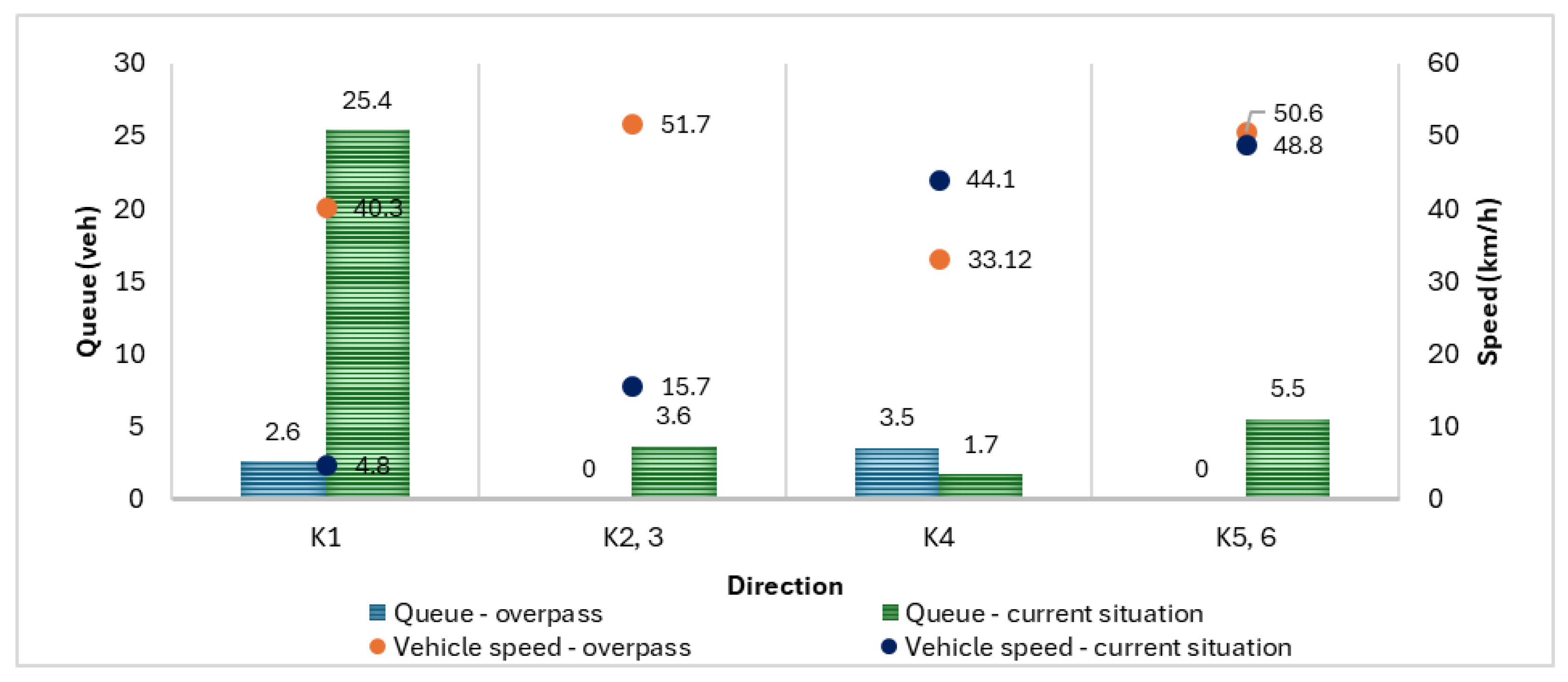
Table 13 show that bridging the main road and creating a roundabout would significantly reduce delay times in all directions. The traffic quality reaches A level in all of the shoulders. The intersection is situated in an urban area, so the maximal permitted speed is 50 km/h and it was not changed in the simulation. Only on the roundabout, the speed limit was set at 30 km/h.

4.6. A Comparison of the Current Situation with Proposed Variants

The simulation was timed from 2 p.m. to 3 p.m. during the peak hour. The graphic comparison between the simulation and the current situation is in Figure 11.

Based on this comparison, the vehicle intensity in individual directions was almost identical. Differences are noticeable only for shoulders A and B, especially for turning left. The green curve represents the green light duration for individual directions.

4.6.1. Evaluation of the Current Situation and Variants I, II, and III

Firstly, the comparison of proposed variants I–III, which are without any geometrical editing of the intersection, was realized. The suggestion for edits in variant III is negligible. In this case, the intersection performance for individual shoulders was evaluated depending on green light duration. On the contrary, variant IV was proposed with a total building layout and compared only with the current situation.

The comparison criteria contained detailed conditions for evaluation and were established as follows:

• Criterion 1: The number of vehicles able to pass through the intersection during the green light duration—green light durations in all directions were considered in this criterion. The number is derived based on the average number of vehicles passing through the intersection in individual directions during the simulation. The criterion applies to established green light duration, but also on the green light duration proportion of the entire simulated hour.
• Criterion 2: Delay time—the delay time was evaluated for individual directions K1–K6 (as they are intended for the measures). The average delay time represents the average value of the time that a vehicle takes to pass the section than it would if there were no other vehicles on the road.
• Criterion 3: Travel time—this represents the average value time needed for passing the observed section for K1–K6 directions. The real time of the travel time depends on the traffic overload.
• Criterion 4: Time loss—the proportion of the average delay time and the travel time. The criterion describes the traffic quality in the observed section.
• Criterion 5: The length of the queue—the average value of the maximal noticed length of queue during the simulation. It is a random variable, a variable over time, and depends on the current traffic flow composition.
• Criterion 6: Average speed analysis—the average speed was evaluated in individual shoulders of the intersection.

Criterion 1 is further evaluated and compared with the current situation of the intersection individually for each variant. Then, the remaining criteria (2–5) are evaluated together.

• Variant I.A

The following Figure 12 visualizes the differences between the number of vehicles able pass through the intersection during the green light duration for individual proposals and the current situation of controlling the intersection. These solutions were determined based on the evaluation of the capacity of TP102 and the intensity of vehicles in individual directions. The controlling cycle of the intersection was prolonged from 70 s to 120 s in this case.

Columns represent the average number of vehicles, and the curve represents green light durations. The highest number of vehicles passing the intersection during the green light duration was noticed in the first solution. The second solution brought the reduction of the number of vehicles passing through in the green light duration in contrary with the current situation. However, Figure 12 reflects the number of vehicles passing through the intersection only during one cycle. Lengths of cycles vary. For this reason, it is necessary to consider the differences noticed in the whole hour.

The cycle 70 s long was repeating 51 times in an hour, while the cycle 120 s long repeated 30 times in an hour. Cycle repetitions reflect the time shares of the green light duration. Vehicle values expressed per hour were determined as follows: for example, the green light duration in shoulder A is 39 s for the current situation. The cycle repeats 51 times and the average was 2.4 passing vehicles during this cycle. These values were multiplied, and the result was 123 vehicles per hour in this direction. However, the green light duration for the same direction during the cycle 120 s long was 60 seconds, and the average was 1.6 vehicles per hour, so the result was 48 vehicles per hour.

The mentioned approach was applied to all calculations of vehicles per hour and for all variants I–III because of the different cycle lengths. These are always vehicle average values.

• Variant I.B

The controlling cycle was generated by the simulation program according to predefined intensities and signal groups.

A prolongation of the green light duration caused the increase in the number of vehicles only in the case of shoulder A (Figure 13). On the other hand, the remaining shoulders stayed the same or decreased. This was similarly reflected in the stagnation of the number of vehicles.

• Variant I.C

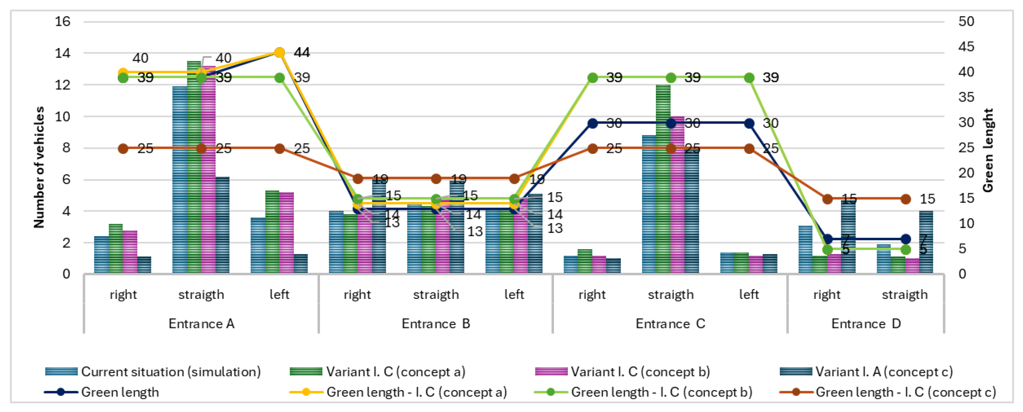
Following calculations resulting from the conditions given in section C—light signal duration optimization based on the mathematical model—three different green light durations for individual phases were specified. Their values are represented in Figure 14.

There are a large number of elements in the image that interfere with each other in Figure 14. For this reason, the green light duration is stated as the same value. For example, the green light duration for concept c is 25 s in shoulder A, but there is only one value for all of the directions. As can be seen in Figure 15, the number of vehicles increased using concepts a and b during one cycle on shoulders A and C, and the decline is minimal on shoulder B. In the concept c, the highest increase in the number of vehicles occurred due to the doubled green light duration, while the effect was completely opposite using concepts a and b. There was a significant decline on shoulder D, and a minimal decline was on shoulder B. Overall, the intersection performance increased more than 9% in the first case (concept a) and in the second case (concept b) by 5.1% compared with the current situation, which represents the values 221 and 123 vehicles per hour. It follows from all this that the intensity or intersection performance should increase slightly if green light duration settings would be based on the concepts a and b.

• Variant II.

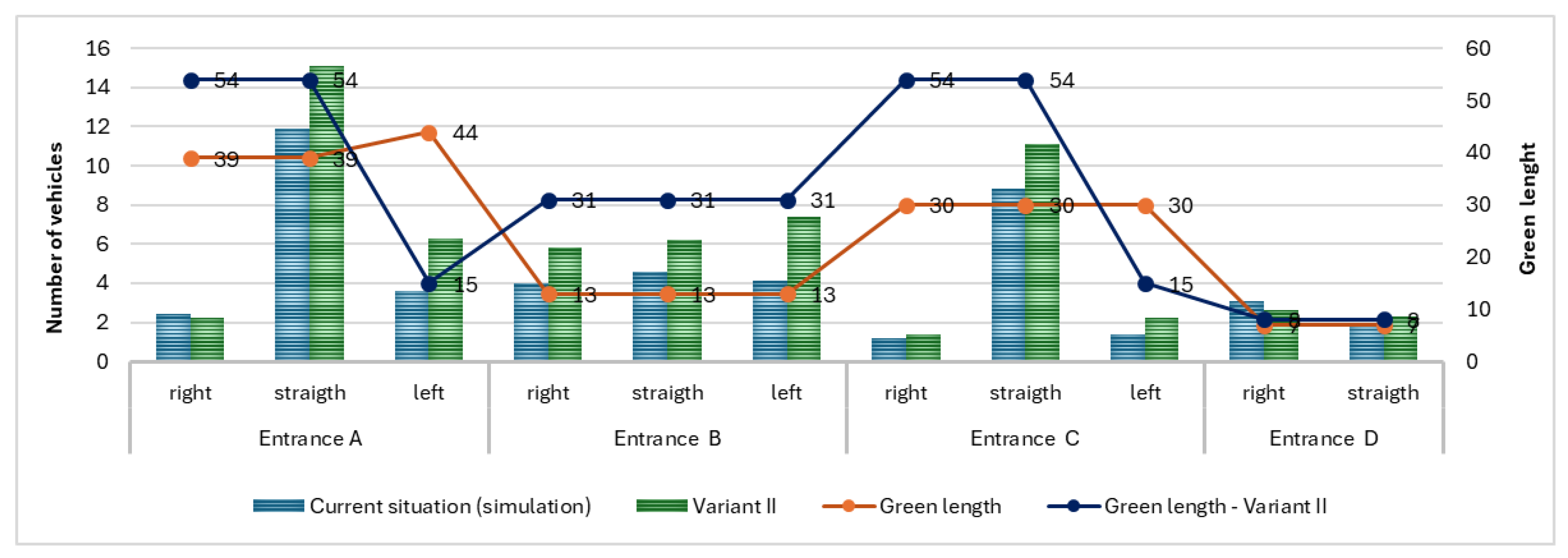
Cars turning left exceeded the intensity of 180 vehicles per hour, so the proposal in variant II was based on the adding of a fourth phase. Traffic overload like this must have an independent phase based on TP102.

The fourth phase consisted of turning left from shoulders A and C (Figure 15). The green light duration decreased to 15 s here, while green signals have longer designed lengths in remaining phases because the controlling cycle changed from 70 s to 120 s. The number of vehicles increased in nine directions of the intersection and in two cases a minimal decline was noticed because of this prolongation. Even then, there was a simulation result, where the intensity increased by a total of 35.7%. However, there is a decline of almost 25% in the comparison of the hourly intensity of the cycles with the current situation. According to the simulation, the intersection is capable of handling 420 fewer vehicles per hour with this proposal of a controlling system. A slight increase in cars turning left in shoulder B and A can be considered as an advantage. The interesting finding is that introducing the separated phase did not cause an increase of cars turning left from shoulder C. The low intensity of vehicles in this direction may be the reason.

• Variant III.

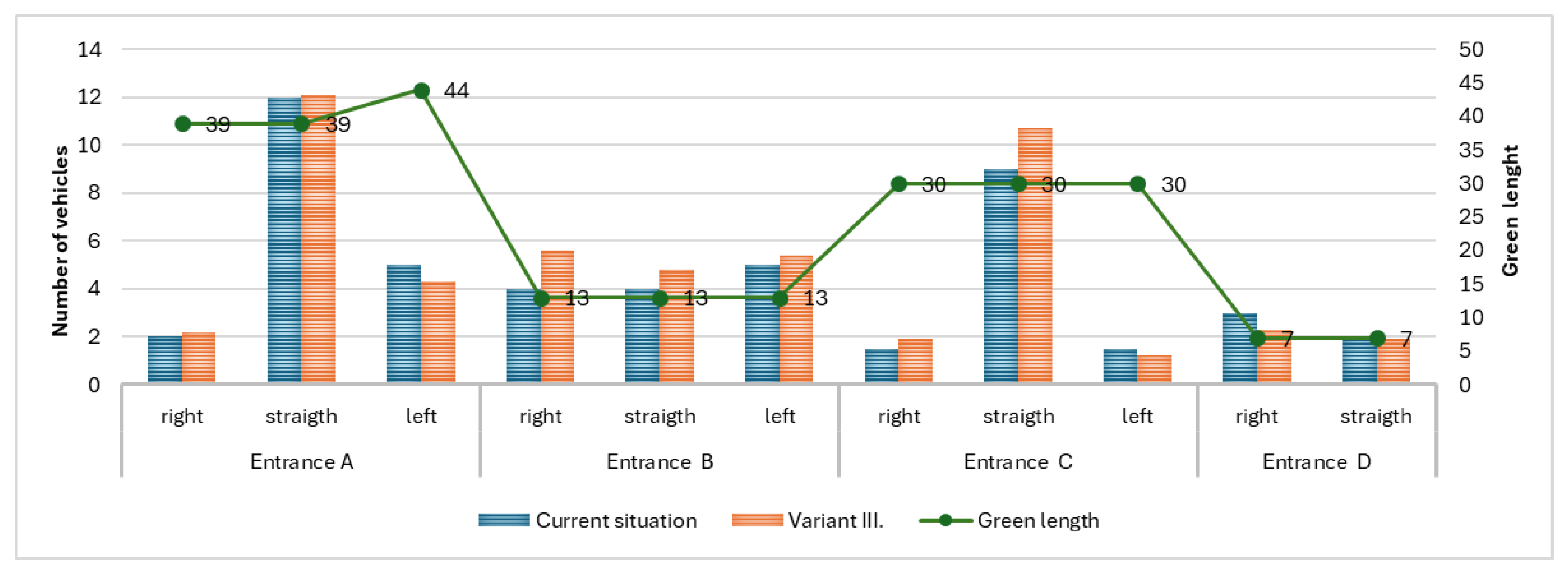
Variant III consisted of the extension of the merging lane to shoulder B. The controlling cycle stayed in the original setting of the current situation.

When the original cycle was left and the merging lane was extended, the intensity of vehicles increased in seven directions (Figure 16). The highest decline was noticed on the straight direction in shoulder D. Compared to the current traffic situation at the intersection, the intensity decreased by 25.8%. The most significant increase in the number of vehicles was found in this case compared with other proposals in the variants. The proposal in variant III brought a positive intersection performance, increasing it by 227 vehicles per hour.

Regarding the optimization of the signal plan, only the calculation according to the mathematical model appeared to be efficient in terms of green light duration and intensity. However, only concepts were considered where a minimum function was required in the form of a delay time. Other variants also did not bring a positive effect in increasing intersection intensity. Using the variant I.A—2nd solution, the intersection performance decreased by almost 45%, which was the lowest result. The highest percentual increasing was shown in variant I.C—concept a by 9.1%. The other two variants (II and III) achieved completely contradictory results: variant II caused a decrease in vehicle intensity by 25%, while variant III brought the most significant increase in intersection performance by 11.7%.

4.6.2. Evaluation of the Remaining Criteria

Criteria 2–5 are evaluated in the following part of this paper. The average values for individual directions (signal groups) were observed, recorded, and used as the basis for capacity evaluation. Directions are marked as K1–K6 (Figure 4). From each simulation, there were exported following average data: travel time, delay time, length of the queue, and speed.

• Delay time and time loss

Time loss was determined as a ratio between the average travel time and delay time in individual directions. For example, the average travel time for the K1 direction in the first solution was 32.7 s and the delay time was 24 s. This resulted in a time loss of 73%. Time loss values in

Table 16. The time loss of vehicles for individual variants.

Time Loss (%)
Direction	Current Situation	Variant I						Variant II	Variant III
		A		B	C
		1. Solution	2. Solution		Concept a	Concept b	Concept c
K1	93	73	84	96	89	85	61	83	29
K2	81	73	89	69	57	57	23	76	75
K3	114	83	96	81	79	80	127	85	83
K4	59	75	64	86	98	99	19	89	11
K5	75	82	86	57	73	77	58	82	73
K6	90	97	93	78	93	91	100	97	89
Average	85	81	85	78	82	82	65	85	60

were determined (in %) by comparing the average delay time and travel time.

The time loss of individual variants is compared to the current situation. The comparison of the proposed variants is evaluated according to time loss (the evaluation of the columns).

The highest time loss was observed for turning left in shoulder C (K3) for the current situation and concept c in variant I.C. Also, Table 16 describes values from the second solution of variant I.A and there are three cases with an increasing time loss. On the other hand, there are three cases with a decreasing time loss in variant III, while the most significant time loss decline was approximately 15%. The stagnation happened in the second solution of variant I.A and in variant II, but there was no increase in the time loss anywhere.

The extension of the turning right lane in shoulder B manifested as the most appropriate variant, just as was proven in the previous comparison for green signals. It can be concluded that each variant had a different effect in individual directions. On the one hand, it brought a decrease, but on the other hand, an increase in another direction. From the tabular processing, therefore, the effective variant among all the proposed variants is variant III.

• The length of the queue and the average speed

The evaluation and comparison of the queue length and average speed in individual directions of the intersection is described based on values in

Table 17. The change of the queue length on the individual directions of intersection.

Queue [veh]
Direction	Current Situation	Variant I						Variant II	Variant III
		A		B	C
		1. Solution	2. Solution		Concept a	Concept b	Concept c
K1	25.4	−11.2	−19	−0.7	−4.8	−8.1	−15.8	−7.8	−24.2
K2	10.9	−6.1	−4.6	−6.7	−7.5	−7.4	−4.6	−0.1	−1.9
K3	1.7	−0.3	0.7	−0.3	−0.3	−0.3	−0.3	−0.1	−0.2
K4	1.7	1.1	0	1.7	11.1	14.5	−1.1	9.4	−1.4
K5	11.5	0.8	1.6	−2.7	−0.2	0.6	8.4	0.6	0.5
K6	11.1	7.6	1.7	−4.2	2.9	5.7	8.4	7.7	0.3
Average	10.4	−1.4	−3.3	−2.2	0.2	0.8	−0.8	1.6	−4.5

.

The largest decreases in the convoy occurred in the K1 direction, with an average of 11.5 vehicles. The current situation was not included in it. The next decreases were noticed in the K2 and K3 directions. However, the application of new proposed solutions in the three directions K4, K5, and K6 also had a negative impact. A positive change in one case may lead to a deterioration of conditions in another one. The evaluation of the criterion showed variant I.B as efficient because it brought the minimal increase only in one direction. However, variant III had the largest decrease of −4.48% and variant II reported a decrease of only −2.15%.

Like the previous criterion, the average speed in individual directions is evaluated. The following

Table 18. The average speed limit of vehicles in individual directions of the intersection.

			Average Speed (km/h)
Direction		Current Situation	Variant I							Variant II	Variant III
		A				B	C
		1. Solution		2. Solution			Concept a	Concept b	Concept c
K1	4.8	28.9		21.4		7.1	13.1	19.8	36.7	21.6	37.9
K2	16.1	25.7		6.9		25.4	32.2	31.7	5.3	22.7	20.1
K3	10.5	16.1		4.3		15.8	16.9	16.2	12.1	15.9	13.2
K4	44.1	38.1		43.6		36.4	13.2	2.5	48.1	13.6	49.9
K5	19.4	20.8		10.5		31.7	20.6	17.5	2.4	19.4	20.9
K6	10.9	3.3		7		19.5	7.4	5.8	0.27	2.9	11.3
Average	17.6	22.2		15.6		22.7	17.2	15.6	17.5	16.0	25.6

contains values recorded after applying all of the changes. The calculation of the average in individual directions did not consider the current situation.

Table 18 above clearly shows that the increase in the vehicles’ speed in some directions could cause the decrease in other values depending on the individual variants. Also in this case, the best alternative was variant III. However, it is important to consider whether the decline occurred in directions that are not overloaded. It is necessary to realize the evaluation of the total intensity of the vehicles, i.e., how many vehicles the intersection is capable of handling with the current situation.

Based on the results of the evaluated criteria, it is possible to draw the following conclusions. Each proposed variant offered different results of the observed indicators. For example, while the speed increased in five directions using variant B, it decreased considerably in others. The positive result brought variant B, where the speed increased in application of each variant. For the final choice of the most appropriate variant as a solution for the intersection, it is necessary to consider several observed indicators, also to determine the significant changes. This condition can evoke a higher vehicle emissions production as well as a lower intersection performance.

As was mentioned above, the most efficient alternative was variant III. Changes related with variant III were positively reflected on traffic organization.

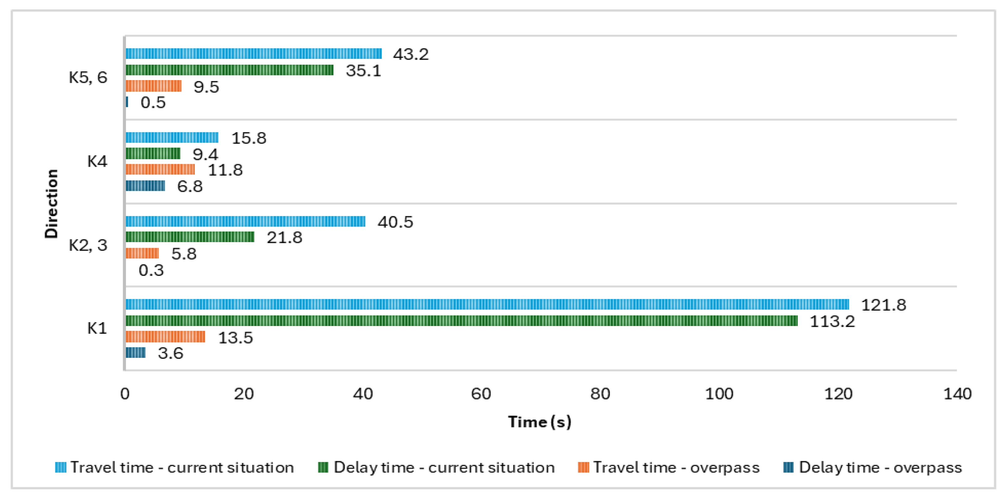
4.6.3. Evaluation of the Current Situation and Variant IV

As a final comparison, the current solution of the intersection and the new building layout are presented. This variant is compared only with the current situation of the intersection because of the complete change in the organization. The criteria were evaluated in different ways because of the changing lanes and character of the intersection. The traffic flow progress was observed only in four directions. The main road was bridged and the rest was transformed into a roundabout. Data are processed and evaluated as seen in Figure 17 below.

In the K1 direction, the observed indicators significantly decreased by almost 96% for delay time and 89% for travel time. The implementation of variant IV to the road network reduced the delay time almost to zero. The blue curve represents the travel time, which decreased an average 70% of all directions. The only downside was a slight increase in the delay time in the K4 direction.

Regarding time loss, the following data were estimated. In the order from K1 to K6 directions, firstly the current situation is 98% and 26%; 46% and 5%, and with the overpass is 59%, 57%, 81%, and 5%. In total, the time loss in individual directions decreased by 47%.

The speed of vehicles in the K4 direction decreased by 24% which could be caused by implementing the roundabout. Vehicles must slow down because of the right of way, while most drivers speed up if the green light is on in their direction at the light signal control intersection. Ultimately, the speed of the vehicles was, in the remaining directions, significantly higher (Figure 18). Where the speed increased, the average queue length decreased. However, it was the most in shoulder B.

4.7. The Choice of the Most Appropriate Variant

Each change in the controlling organization of the intersection is realized with a certain intention, like the increasing of safety, the eliminating of negative impacts, or increasing traffic performance. The intention has always its risks and benefits, but the goal is to achieve a certain quality level. In terms of transportation, the quality represents a fluent traffic flow. For this reason, speed, transit time, delay time, the length of the queue, or the number of stops are key terms. The intersection performance can be determined as the maximum number of vehicles that an intersection can pass in a certain time unit (e.g., peak hour).

In following

Table 19. The output results simulation of variants for the determination of the quality and performance of the intersection.

Direction	Current Situation	Variant I						Variant II	Variant III.	Variant IV.
		A		B	C
		1. Solution	2. Solution		Concept a	Concept b	Concept c
Delay time [s]	90.48	96.2	96.32	84.26	90.32	98.94	107.45	133.45	35.08	7.81
Wait time [s]	75.91	76.14	71.58	72.09	77	84.43	93.23	109.96	25.47	1.42
Travel time [s/km]	142.27	148.26	149.63	135.99	142.11	150.71	161.2	185.5	87.05	60.8
Number of stops [#/veh/km]	0.18	0.15	0.22	0.15	0.14	0.14	0.23	0.19	0.08	0.02
Density [veh/km]	15.67	19.02	20.06	14.45	14.94	15.99	25.95	21.11	11.46	8.41
Intensity [veh/h]	2013	1892	1945	1997	2027	2001	1161	1844	2057	2055
Speed [km/h]	39.7	36.02	30.24	46.36	42.42	40.99	36.01	32.61	47.1	61.02

, results of the intersection performance in simulations of all of the variants are compared.

The delay time reached the highest positive change in the case of the variant IV application and on the contrary, variant II become the lowest. The wait time increased by 45% after introducing the fourth phase (variant II) and decreased the most by 98% with variant IV.

The travel time and number of stops achieved the highest positive change again with variant IV. The travel time increased the most in the case of variant II by 43 s compared to the current situation. However, the number of stops, at a value of 0.23 for one vehicle per kilometer, was recorded in the simulation using variant I.C—concept c. This variant used the mathematical model. The condition was formulated as follows: the maximal value from the mean vehicles waiting for the green light turned on and the sum of the mean values of the total unused green light time was minimal.

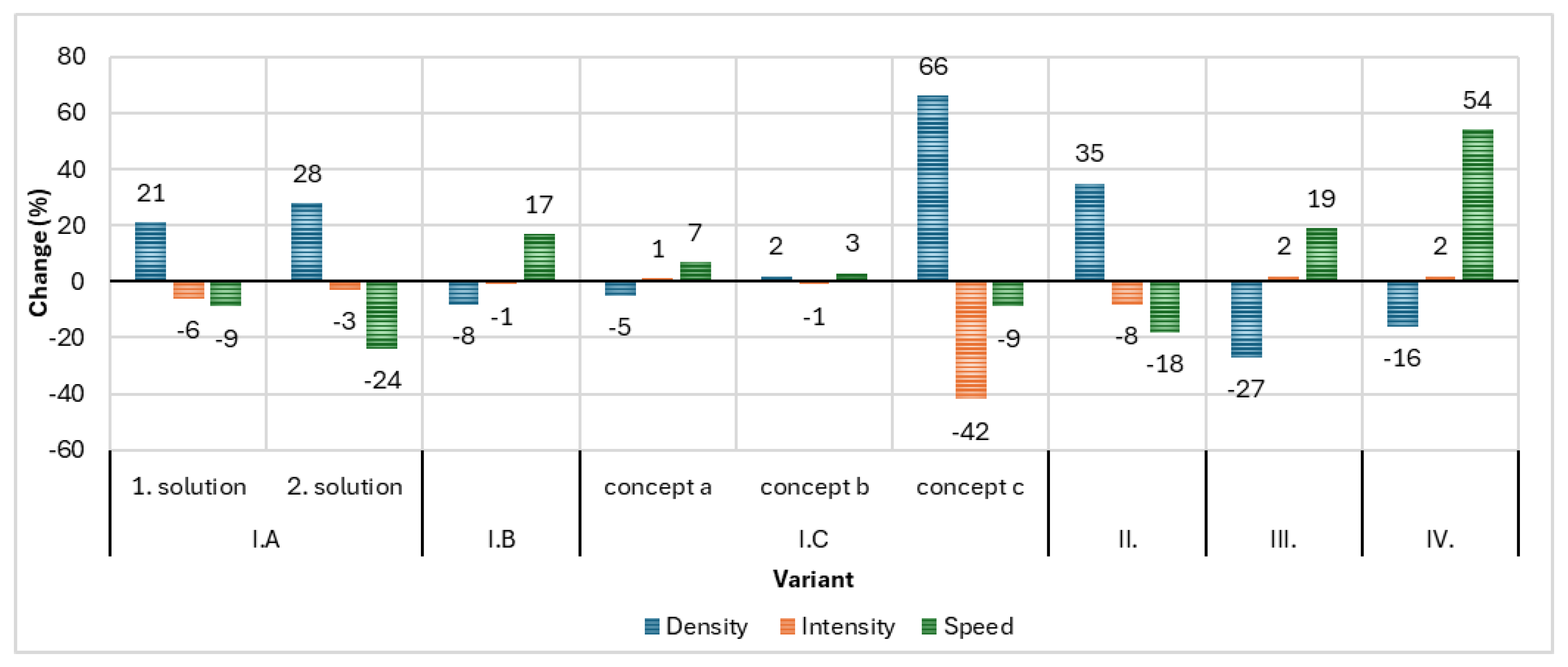
How intensity, speed, and density influence each other is based on known facts, and it is depicted in Figure 19. The changes compared to the current situation (horizontal axe) are expressed in percentage. Variants with an intensity reduction recorded also a reduction of traffic speed. This phenomenon in turn caused an increase in the number of vehicles on the length units, so density. Because of the linear relation between the speed and density, the reduction/increase in one value is reflected in the increase/reduction in another one. However, the relations between traffic density and intensity, and intensity and the speed of vehicles are described by parabola. The observed value increases until a certain point when it reaches an optimum (vertex). Afterwards, they start to decline even though the second value still increases.

Four variants brought positive changes compared to the current situation: I.B, I.C—concept a, III, and IV brought the most significant positive changes. The first two variants mentioned also achieved a negative change in one criterion, but only by 1%. The simulation output values for concept c in variant I.C and variant II were reflected in a negative result. In variant I.C, the deepest decline in the intensity at −42% caused a rapid increase in density by 66%. The lowest intersection performance was recorded in this case (1161 vehicles/h). An increase of intensity occurred only in three variants—concept a in the I.C variant, then variant III and variant IV. The speed increased in five cases, but the most significant was in the last variant by 54%. From an overall perspective, two variants brought positive results and two brought negative results (Table 19). The largest negative average deviation of changes relative to the current situation was brought by the concept c and variant IV was shown as the best one. However, considering the costs associated with its implementation, it would be variant III.

5. Discussion

The proposed variants were based or inspired by scientific articles and publications. The signal plan optimization was used for the first proposals. Most of these studies [36,37,38,54] realized the optimization based on the four basic parameters of signal plans (the length of the cycle, the green light duration, the sequences of phases, and yellow lights) like in this paper. The optimization brought only two from four variants which reported a delay time reduction, but only less than 1% while the delay time in the mentioned studies reduced in the range 15–18%. Even authors in [33] stated the delay time reduced by 35% using the optimization of the signal plan. Used methods were established as follows: the optimal length of the cycle as the function of time loss and the intersection intensity ratio, and optimal light signal settings depending on the reduction in delay time. Many studies with this aim have been tested with VISSIM software [55,56,57]. The optimization of the green light duration in our research was realized using the calculations from TP102, generated by Aimsun version 8 software for creating the simulations and defined by the mathematical model conditions in [52].

Variant I.B was the best option in terms of optimization. Variant II resided in the optimization by adding the new phase (fourth phase). The optimization consisted of 24 combinations of solutions with the minimal intersection yellow light time. However, the delay time increased more than by half in this case. The delay time represents on average a more than 46% travel time based on the meta-analysis in [58].

The travel time depends on several factors: drive or vehicle characteristics; the interactions between drivers in a traffic network (like the heterogeneity of other drivers and their vehicles); traffic rules and the system of traffic control; and weather conditions. In the current situation, the delay time reached 65% in the case of selected intersection. The application of the proposed variants gradually reduced, stagnated, or increased slightly the delay time. In addition to monitoring outputs, attention was focused on the average number of vehicles that manage passing through the intersection during the green light in each direction. Despite the decline of intersection performance, the number of vehicles passing during the green light duration at individual directions increased in some cases. This increase concerned directions with a short green light duration. According to this finding, the intensity of the intersection did not increase on the most loaded shoulders, and so it led to the decline of intersection performance.

Variants III and IV contained a geometric editing of the intersection. The merge lane extension/prolongation reduced the delay time by 60%.

However, as other research suggests [42,45], building the overpass represented the most appropriate proposal. A study with the aim to overcome problems with main intersection overloads in the city Palembang proposed the application of the underpass and overpass. Microsimulation software VISSIM was used for the evaluation of the intersection performance in the traffic network with compared parameters like the length of the traffic queue and the average delay. Realized modelling and results of the analysis showed that the optimization of intersection performance was construction editing and traffic diversion. Also based on the study [42], the permanent solution for efficient intersection performance requires the overpass which increases the speed of vehicles four times faster. The delay time after the application of variant IV declined by 92% and the speed of vehicles significantly increased. Time savings are often considered one of the biggest benefits in transportation projects. Researchers and experts assume that travel is derived from demand in the calculation of the time savings in traffic (based on a given formula of origin and destination) and that the travel time used to be marked as “disutility” in economics (something that people want to minimize) [59].

The influence of time changes on the whole traffic network is related to the travel time for work or private purposes. However, the greatest influence reflects especially in the transporting of cargo that may also have a time value. These are trucks where the shipper or recipient bears excessive costs for a late pickup or delivery [60,61]. The travel time variability loss caused by unpredictable occurrences increase also operational costs of trucks (for example fuel consumption) and from this comes another form of cost, an environmental externality.

6. Conclusions

The proposed solutions were developed on the basis of extensive expert studies dealing with the solutions of problematic traffic situations. Aimsun version 8 software was used to verify the proposed solutions, which allowed the creation of individual simulations. The proposed solution variants included the optimization of the signal plan, as well as geometric adjustments to the current traffic management layout.

The aim of all of the proposed variants was to reduce delay times and increase the performance of the intersection.

However, not every solution turned out to be positive. The results showed that geometric adjustments can most significantly improve the performance of the intersection. The construction of a main road overpass turned out to be the most suitable variant. This solution would significantly affect the current state of the intersection. Regarding the selection of the proposed recommendation, the overpass achieved the best results within the observed and evaluated values. The vehicle speed increased significantly and the vehicle density at the intersection decreased.

The results of this study provide a useful resource for urban transport planners and policymakers to predict and address the effects of road modifications. Limitations and future research directions are as follows:

Simulation Time Limitation: The simulations were conducted for only one peak hour, which may not represent the full day’s variability of the traffic situation. Peak times may vary at different times of the day and on different days of the week.

Neglect of External Factors: The research primarily focuses on the intersection itself and does not consider the possible impact of external factors such as nearby traffic accidents, road closures, weather, or seasonal changes in traffic flow.

Lack of Economic and Environmental Assessments: The research focuses on the technical aspects of traffic flow and does not assess the economic costs of individual solutions (e.g., the cost of constructing an overpass) or their impacts (e.g., emissions).

The symbiosis between the basic characteristics of the traffic flow is possible by rationally controlling and so on, creating more ecological as well as more well-performing solutions not only at the selected intersection, but in the whole traffic system.