1. Introduction
A rapidly growing number of urban systems and services require the provision of Positioning, Navigation, and Timing (PNT) services [
1,
2]. Urban systems and services are increasingly utilising the Internet of Things (IoT) to form smart buildings, smart cities, Intelligent Transport Systems (ITS), and similar complex systems [
3,
4]. Those require precise, robust, and resilient position determination processes of mobile and stationary objects, as well as accurate timing synchronisation service [
1,
2]. The majority of urban systems and services utilise mass-market, single-frequency, commercial-grade GNSS receivers [
3,
4]. As utilisation usually focuses on planar applications, horizontal positioning accuracy is of the prime concern.
The Global Navigation Satellite System (GNSS) is a constellation of four interoperable global systems, comprised of the GPS of the United States of America (USA), GLONASS of the Russian Federation, Beidou of China, and Galileo of the European Union [
5,
6]. The GNSS positioning performance varies in relation to positioning environment conditions [
5,
7], which are determined by natural (space weather, geomagnetic field, ionosphere, and local multipath environment) and artificial sources of disruptions and degradations (GNSS spoofing, jamming, and meaconing) [
8,
9]. The mitigation of the GNSS PNT degrading effects is performed through a range of methods, including the utilisation of advanced hardware and the implementation of statistical correction models.
Among the various disruptions to PNT services [
5,
6,
7], ionospheric conditions are a leading natural cause of degraded GNSS performance. The ionosphere represents the most significant natural challenge to robust GNSS operation [
8,
10,
11]. Ionospheric delay is a key contributor to GNSS pseudorange measurement errors and [
12,
13,
14], by extension, to the overall GNSS position estimation error budget [
15,
16,
17]. This affects GNSS positioning accuracy indirectly through the introduction of a GNSS signal propagation delay [
5,
18], which is incorporated into the positioning algorithm [
6,
7,
10]. The GNSS ionospheric delay is the result of the physical processes in the upper atmospheric charged layers, resulting in slowing down the satellite signal [
7,
10,
11] and rendering it to appear as travelling a larger distance [
12,
19]. The GNSS ionospheric delay is defined by a simplification of the Appleton-Hartree equation [
7], given in Equation (
1), which associates the GNSS pseudorange measurement error
of a satellite signal transmitted at the radio carrier frequency
f with the vertical ionospheric profile
, a surface density of charge particles at height
h above the mean sea level of the Earth [
7,
11,
12].
The integral on the right side of Equation (
1) is known as the Total Electron Content (
), a result of the ionospheric conditions [
5,
7,
11].
is directly proportional to the GNSS pseudorange measurement error
[
6,
7,
11].
The problem of the GNSS ionospheric delay [
5,
6,
7] lies in its complexity [
8,
10,
11], as the result of numerous processes [
12,
20] determining the ionospheric conditions [
19,
21]: space weather conditions and disturbances, geomagnetic conditions and disturbances, natural phenomena resulting from their effects to the atmosphere (Travelling Ionospheric Disturbances (TID) [
22], Sudden Ionospheric Disturbances (SID) [
7,
11,
13], Acoustic Gravity Waves (AGW) [
23]), as well as natural (earthquakes [
24,
25,
26], volcanic eruptions [
7]) and artificial terrestrial (ultrasonic flights [
6,
7]) phenomena.
The complexity of GNSS ionospheric delay [
5,
6,
7] and positioning error [
10,
12] is expressed in terms of systematic (bias and seasonality) and stochastic (variance) components [
19,
20]. Research in the field has yielded standard global GNSS ionospheric correction models, such as the Klobuchar model for GPS [
19], and its derivatives for GLONASS and Beidou systems [
5,
6]. The global GNSS ionospheric correction models exploit the identified daily pattern of the systematic component of
and GNSS ionospheric delay [
5,
6,
7], while averaging the situation by using the experimental
measurements taken across the globe [
10,
12,
19], as depicted in
Figure 1.
The shortcomings of standard global GNSS ionospheric delay models lie in [
5,
6,
10,
12,
13,
19] (i) their inability to respond to fast-developing ionospheric disturbances, as model parameters update on the daily basis, (ii) inability to respond to local, or spatially constrained events, as they extend the global ionospheric situation, (iii) still retain the random and partial systematic error uncompensated for.
A dual-frequency GNSS receiver may compensate the ionospheric delay almost in full by estimating the
, and GNSS ionospheric delay, using the model depicted in Equation (
2), where
and
denote two different GNSS carrier frequencies used for simultaneous pseudorange measurements (for GPS,
MHz,
MHz), and
denotes the difference between pseudoranges measured at
and
, respectively [
5,
6,
10,
12,
13].
However, a vast majority of GNSS receivers, especially those of the mass-market nature applied in urban systems and services, utilise a single-frequency GNSS positioning process, thus requiring the mitigation of the ionospheric effects [
10,
12,
13].
Inaccurate measurements [
5,
6] of the distance that the GNSS signal travelled cause the GNSS position estimation error [
10,
19,
20]. The error sources affect the accuracy of the GNSS pseudorange measurements through the introduction of GNSS pseudorange measurement error
[
5,
10], which maps onto the GNSS position estimation error
as given in Equation (
3) [
12,
13].
The matrix
G is defined with Equation (
4), with position components of satellites whose signals are used in the positioning algorithm (index
) [
5,
6], and the user/GNSS receiver position (index
) estimated in the positioning algorithm’s
i-th iteration [
10,
12].
The variable
depicts the distance between the estimated user position in the observed iterated step of the positioning algorithms, and the position of the related
n-th satellite [
5,
6,
10].
It is essential to recognise that the GNSS ionosphere delay is not directly proportional to, but rather mapped into, the GNSS positioning error, as expressed in Equation (
3) [
10,
12].
Further developments in GNSS resilience against ionospheric effects, the major single cause of GNSS PNT degradation, rely on the further identification of GNSS positioning errors [
5,
6,
10] caused by these effects [
19,
20]. The resilient GNSS may contribute to significant improvement of the Quality of Service (QoS) of both the critical and mass-market [
1,
2] urban systems and services [
3,
4,
10].
The unaccounted (un-modelled) bias and seasonality, as well as the inability to account for the random component and short-term local ionospheric disturbances, render the existing GNSS ionospheric correction model [
8,
10,
12] inadequate for modern high-accuracy GNSS applications [
19,
20], as depicted in
Figure 1. The introduction of novel approaches in GNSS ionospheric delay model development and operation, through the utilisation of the ambient awareness and an active role of the particular GNSS application in setting up and operating the GNSS positioning algorithm, offers a much-needed breakthrough in mitigation of the most prominent source of GNSS positioning performance degradation [
10,
12]. The implementation of the Ambient-Aware and Application Aligned
GNSS positioning service requires the assessment of the GNSS ionospheric delay dynamics and GNSS positioning performance from the new perspective of the individual GNSS PNT unit (rover) stationed in real positioning environment (ambient) conditions at a certain place in the world [
10].
Here, we propose a novel approach [
20,
21,
27] to the personalised assessment [
28,
29] of long-term GNSS positioning performance using Recurrence Plot Analysis (RPA) [
30,
31,
32] of experimentally collected raw GPS positioning observations from a horizontal GNSS positioning experiment. These observations were obtained using a commercial-grade single-frequency GNSS receiver and sampled at a rate of 30 s. The proposed approach is demonstrated in the case of an International GNSS Service (IGS) reference station in the sub-equatorial area, which collected GPS pseudorange observations throughout 2014, thus forming a database of raw GPS observations containing the ionospheric effects in their actual depths and rates of occurrence. Pseudorange observations of the other GNSS systems are not used to focus the study on performance issues and avoid additional inter-system issues.
The presented research considers the GNSS positioning error caused by ionospheric effects from the perspective of applications [
1,
2] and users [
3,
4,
10]. The selection of the horizontal GPS positioning error in the presented study results from the importance of the performance indicator for the vast majority of GNSS applications [
1,
2] in urban systems and services [
3,
4]. Additionally, the results presented here, reverse-engineered to
analyses, may inform the formulation of multidisciplinary monitoring frameworks that integrate GNSS with geophysical hazard assessment, including seismic precursor studies. Such research remains outside the focus of the presented research.
The contribution of the presented research is in setting up and applying the RPA framework that maps the Disturbance storm-time (Dst) index, a descriptor of intensity of geomagnetic activity [
7,
33,
34], and horizontal GPS positioning error values to well-known classes of recurrence plots, thus revealing potential associations between variables concerned.
The identified associations, predicting variables, and the RPA parameters indicating the identified non-linear processes in horizontal GPS positioning errors may be integrated into resilient GNSS PNT algorithms, where applications adapt dynamically to environmental conditions. This results in a resilient GNSS capable of servicing urban systems and services with enhanced positioning performance, as well as a more robust and improved QoS.
2. Materials and Methods
This section provides a data description and outlines the methodology used in the research. The presented research is performed using code developed by the authors in the open-source R(v. 4.5.1) environment for statistical computing [
35].
The research aims to develop an innovative application of RPA to characterise the nonlinear dynamics of GNSS errors. Traditional studies often focus on statistical measures such as variance. The presented research reveals commonly neglected nonlinear patterns and behaviours of GNSS errors that can be used to improve existing error correction methods and models, rendering GNSS PNT more resilient and sustainable for a growing number of GNSS applications. The research aim is to contribute to setting a development framework for new GNSS PNT positioning methods by understanding the nonlinear dynamics of horizontal errors. The conclusions the authors present are not the end of the process, but rather a starting point for the development of more robust algorithms in the future.
The presented research provides justification for its contribution to the development of sustainable GNSS, thereby rendering GNSS-based urban mobility systems and services more sustainable.
The GNSS pseudorange observations used in this study were obtained from the International GNSS Service [
36], an open-access repository of voluntarily provided high-quality GNSS data, which serves as the primary data source for research. Access was performed through the National Aeronautics and Space Administration (NASA) Crustal Dynamics Data Information System (CDDIS) repository [
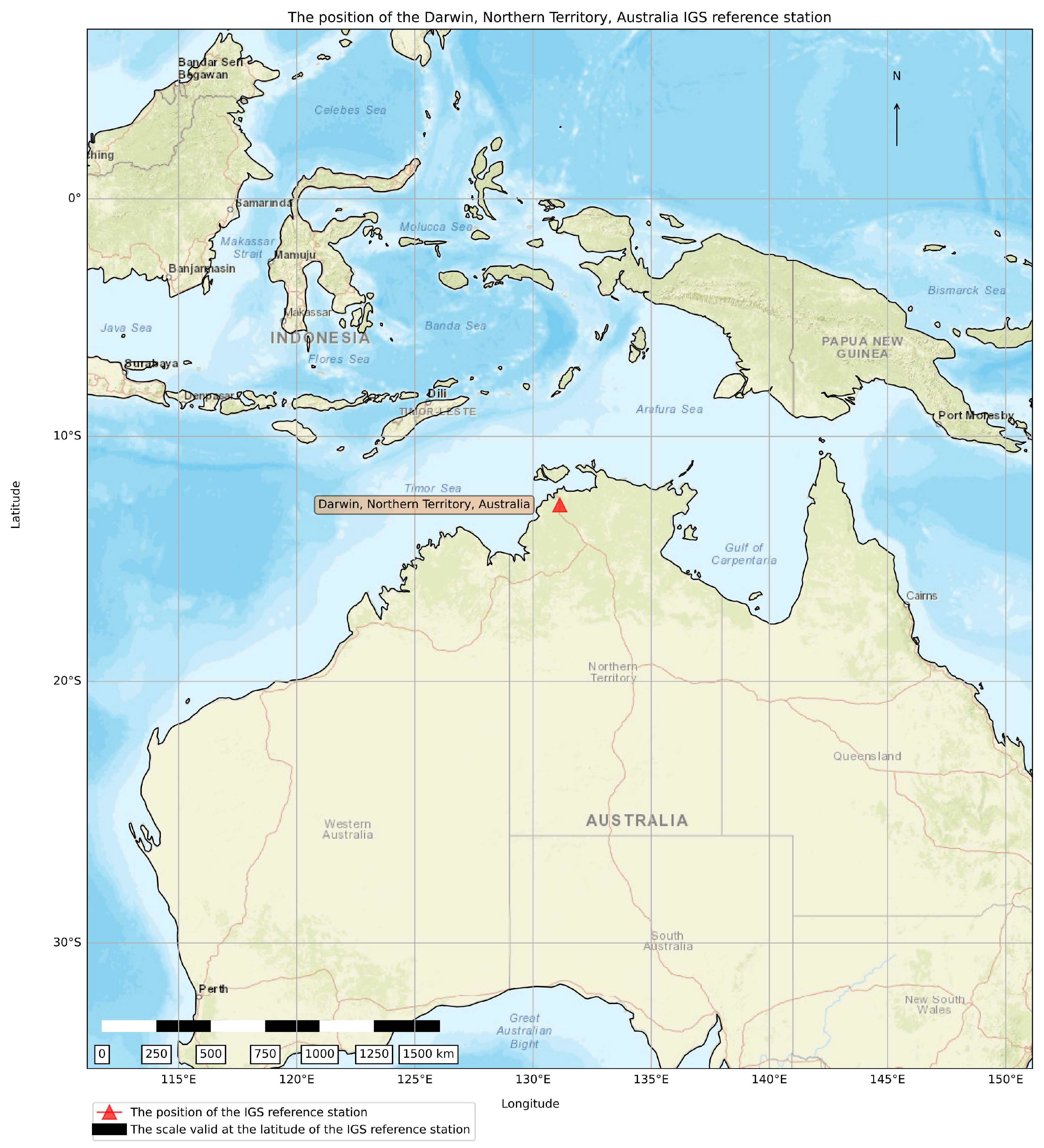
36]. The Darwin, Northern Territory, Australia International GNSS Service (IGS) reference station in
Figure 2 was selected as a source of GPS observations from a sub-equatorial region. The presented research aims at the methodology definition and identification of non-linear dynamics of the GPS horizontal positioning error, considering data collected at a single point (IGS Darwin reference station) in the sub-equatorial region known for its exposure to extreme ionospheric conditions. This research argues that in such a scenario, non-linear dynamics of the GPS positioning errors may be identifiable, and as such usable for further research on the enhancement of the GPS/GNSS resilience against the ionospheric effects.
Research material consists of GPS dual-frequency raw and uncorrected pseudorange observations (structured as RINEX
files) and the received GPS navigation messages (structured as RINEX
files) collected with a 30 s sampling rate for each day in the year 2014 at the IGS reference station at Darwin, Northern Territory, Australia [
36], with precisely known position. The antenna used at the Darwin IGS reference station is a LEICA choke-ring antenna, specifically a LEIAT504, which is designed to mitigate multipath effects and provide high-quality observations.
The 30 s sampling rate has been selected by the ionospheric researchers and organisers of the IGS network, and set as the IGS standard, thus allowing for the detection of fast-developing ionospheric disturbances and the provision of sufficient granularity of observations for further analysis of ionospheric conditions and their effects.
We processed the raw data in post-processing mode using RTKLIB (open-source GNSS software-defined receiver) [
37]. The receiver was configured as a single-frequency, commercial-grade GPS unit, which represents the dominant class of devices in smartphones, IoT systems, and consumer navigation. While dual-frequency receivers can mitigate ionospheric delay directly, our choice reflects real-world constraints of urban GNSS applications, where low-cost, single-frequency devices are prevalent.
To ensure transparency, we summarise the RTKLIB processing parameters in
Table 1.
The presented study is concerned with the GPS performance of a single-frequency commercial-grade GPS receiver as the prevailing class of the GNSS receiver adopted particularly in the mass-market devices (smartphones, IoT devices) that support urban systems and services. The RTKLIB post-processing utilises the procedure for the GPS position estimation based on the experimental raw (uncorrected) GPS pseudorange measurements taken at the IGS reference station Darwin. A standard GNSS receiver would correct the raw GPS pseudorange measurements for ionospheric effects using the proprietary correction model (Klobuchar [
19] for GPS). As this research aims at addressing the non-linear properties of the horizontal GPS positioning error, the GPS position estimation is performed with the raw (uncorrected) GPS pseudoranges. The targeted scenario is set through a suitable configuration of the RTKLIB post-processing. The GPS position estimation is accomplished through the utilisation of the common algorithm, described elsewhere [
5,
6,
8]. It yields GPS positioning estimates (samples) used for deriving the northing and easting positioning errors, and consequently, the horizontal GPS positioning error, with reference to the precisely known position of the IGS GNSS receiver.
The northing and easting were converted to horizontal positioning errors using the known correct longitude and latitude of the station, which are
° E and
° S, respectively. The conversion of longitude measurements to errors [m] is performed according to Equation (
5), while the same procedure is demonstrated in Equation (
6) for the latitude values. The horizontal error [m] is calculated using Equation (
7) implemented in a tailored software developed by the authors in the R environment for statistical computing [
35]. The data preparation methodology is elaborated upon with more specification in previous publications [
10,
19].
The presented study assesses the association between space weather and geomagnetic conditions, as well as horizontal GPS positioning error, through an additional analysis of Dst-index time series dynamics [
7,
10,
12]. Disturbance storm-time (Dst) represents an averaged measure of geomagnetic storm intensity in the Earth’s sub-equatorial region [
7]. The presented study utilises Dst data taken from the internet-based archive INTERMAGNET [
34].
To advance understanding of GNSS performance under disturbed ionospheric conditions, we apply RPA, a methodology originally proposed by Poincaré [
28] and later developed into a robust framework for studying complex systems [
31]. The RPA [
27,
28,
29] nonlinear time-series analysis technique is applied to both horizontal GPS positioning error and Dst-index time series in the presented study [
30,
31,
38].
RPA plots are a technique of visually representing when a system’s state returns to a previously visited region in its phase space in two dimensions. This method allows for the detection of hidden periodicities, stochastic behaviours, and transitions in error dynamics that are not evident in traditional statistical measures. This allowed us to characterise the nonlinear associations between geomagnetic/ionospheric activity and GNSS performance, a key objective of our work.
The specific objectives of this study are to characterise the nonlinear dynamics of GNSS horizontal positioning errors in sub-equatorial conditions, compare these error dynamics with the behaviour of the Dst-index, evaluate the potential of RPA variables such as recurrence rate, entropy, and trapping time as indicators of GNSS performance degradation, and demonstrate the urban relevance of these findings for resilient GNSS operation in mobility, IoT, and smart city services.
Quantitative descriptors of recurrence plots, known as Recurrence Quantification Analysis (RQA) measures, include the Recurrence Rate (), the proportion of recurrent states, Determinism (), the proportion of points forming diagonal structures, Entropy (), the Shannon entropy of diagonal line distributions, Laminarity (), the proportion of points forming vertical structures, and the Trapping Time (), the average length of vertical structures. These variables provide nonlinear indicators of system stability and transitions.
After collecting all the data, both the horizontal positioning error and Dst are analysed using the RPA variables, as follows in
Table 2. The RPA variables used for the quantitative analysis are summarised in
Table 2, and their formal definitions are given afterwards.
The percentage of recurring points in the radius named
(
) is shown in Equation (
8).
The fraction of recurring points in diagonal lines (
) is presented with Equation (
9).
The total count of lines in the generated plot is recorded as the variable. We also calculated the average line length (L) to describe the typical duration of similar behaviours within the system’s dynamics.
The Shannon entropy (
) of the total of
diagonal lines with lengths larger than the minimum threshold is computed using Equation (
10).
The percentage of recurrent points in vertical lines (
) is defined by Equation (
11).
The average length of visible vertical lines (
) is expressed in Equation (
12).
After the first screening, the RPA settings were determined, with the most impactful to RPA given these values: .
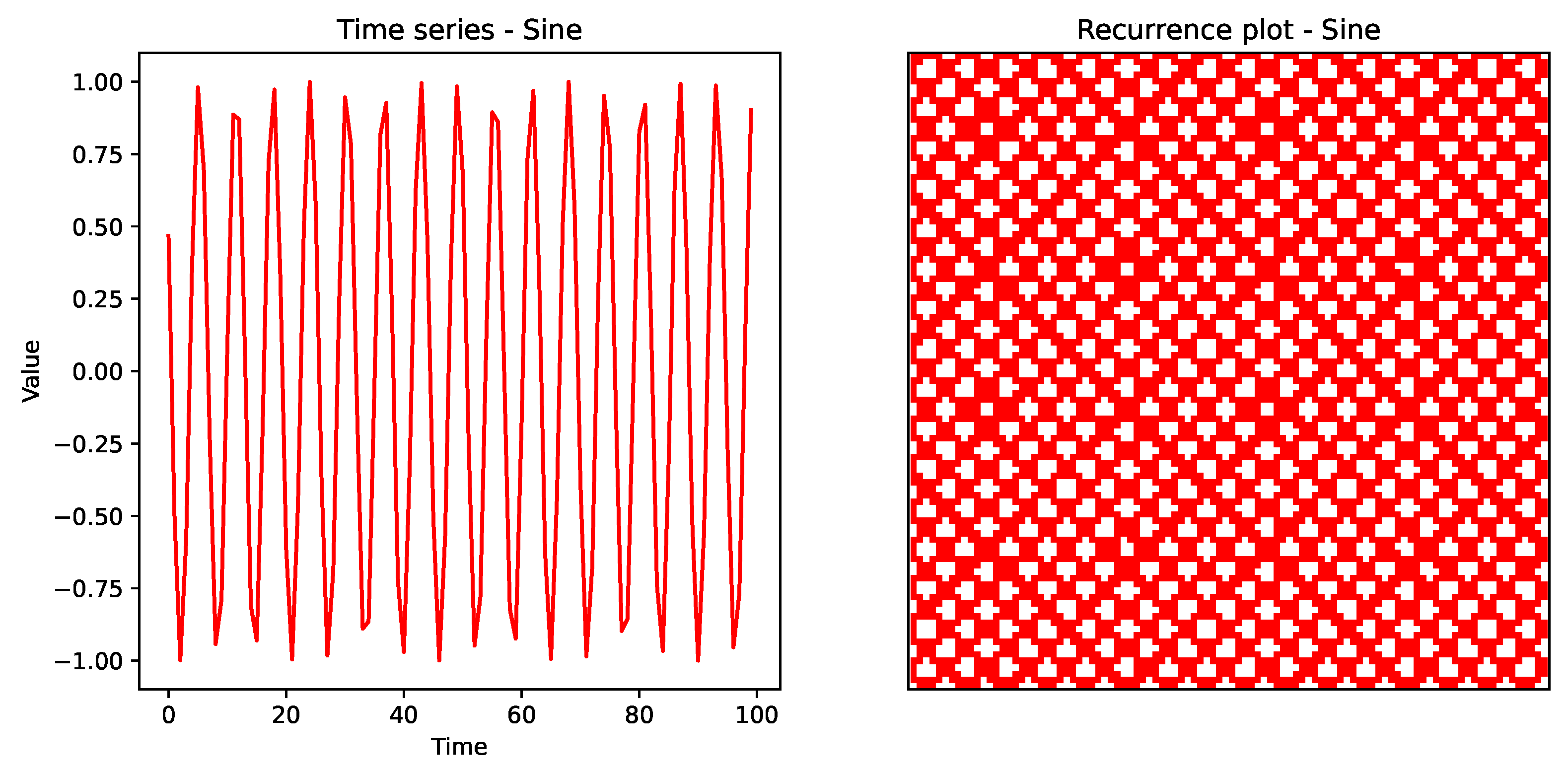
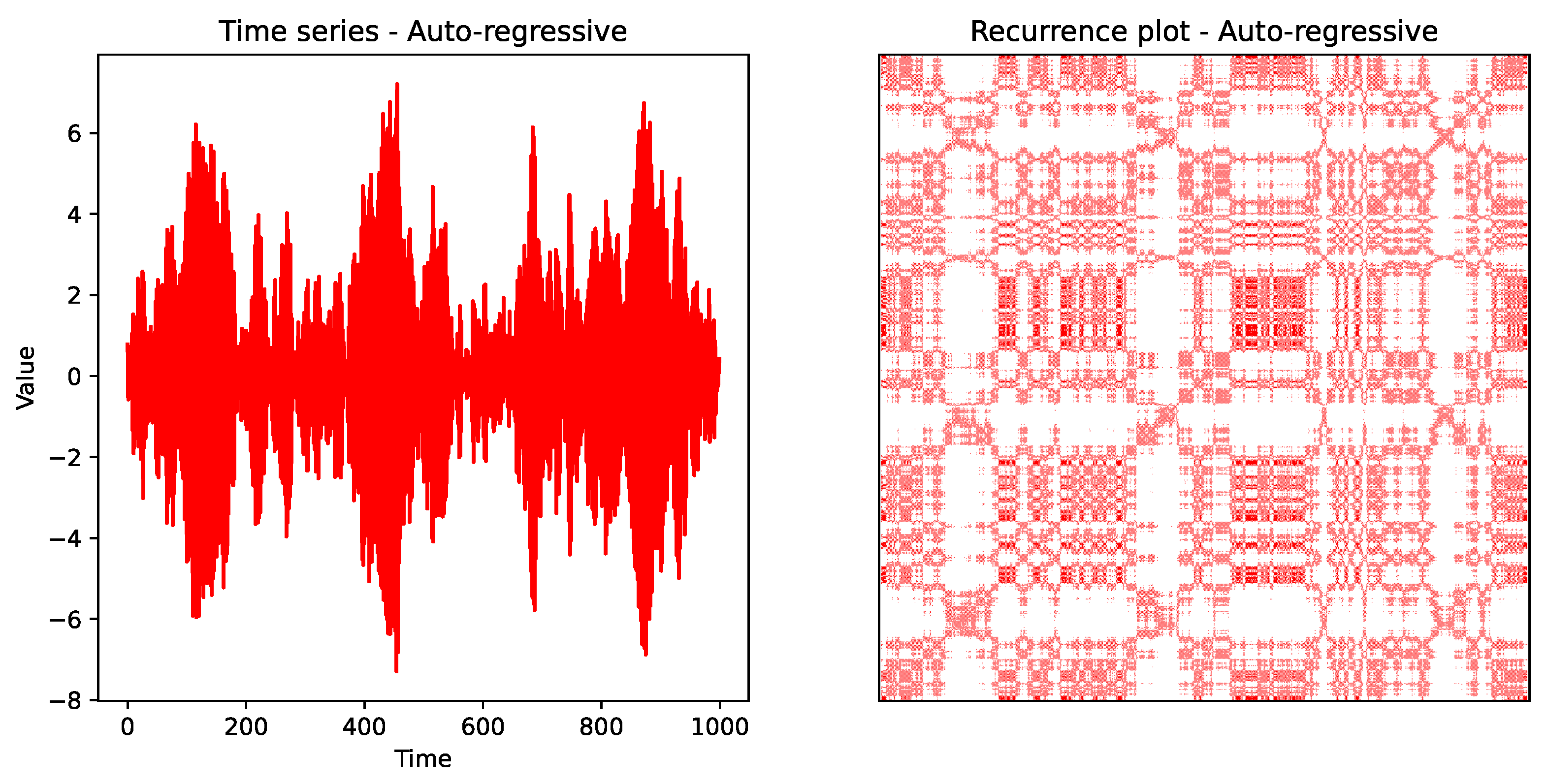
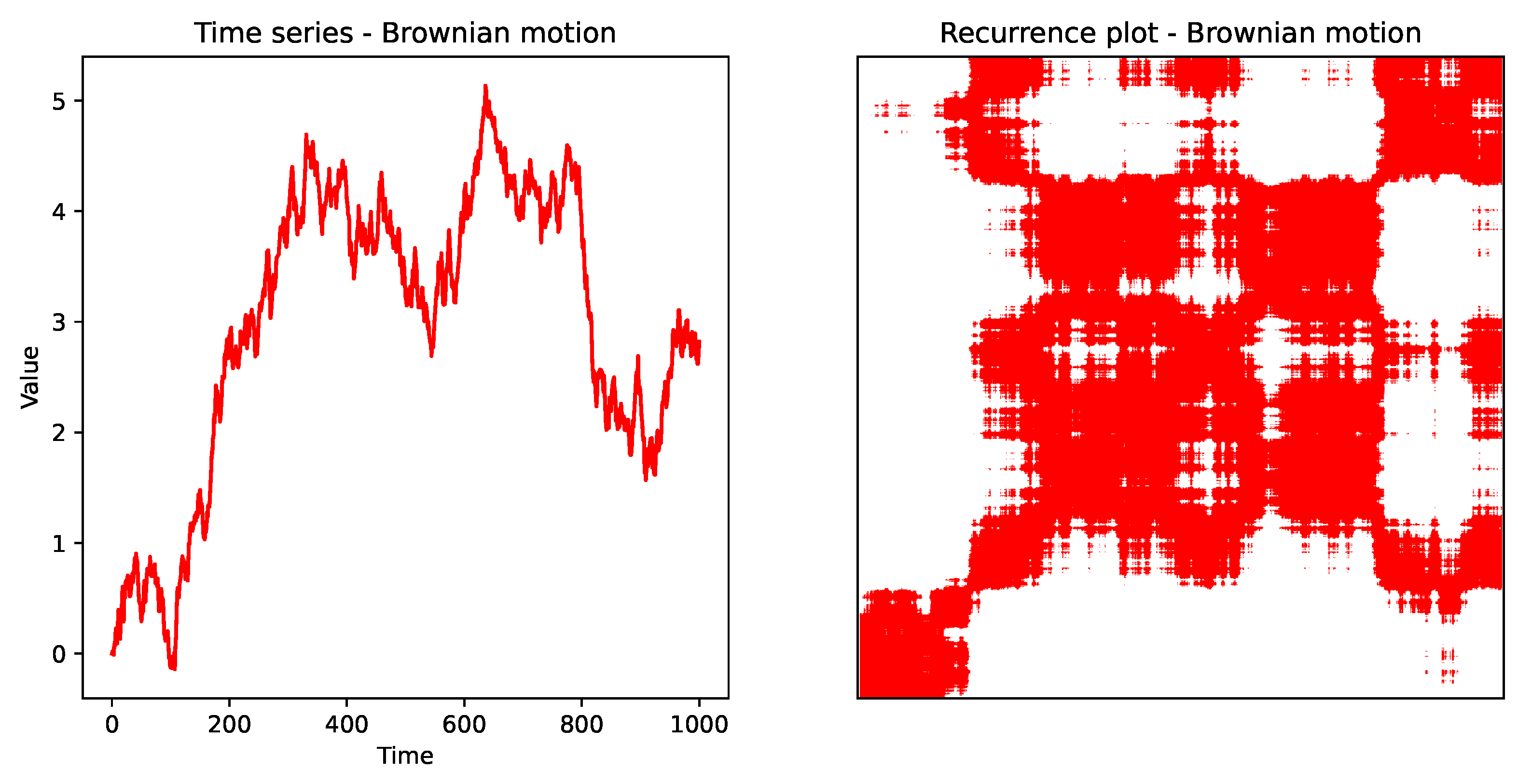
To validate the recurrence plot methodology, we first applied RPA to a set of canonical time series, including the sine function, Gaussian white noise, Brownian motion, auto-regressive (AR) processes, and logistic maps. These examples represent typical nonlinear dynamics and provide a baseline for interpreting GNSS error time series. The sine function recurrence plots show periodic diagonal structures, reflecting oscillatory behaviour. The white noise recurrence plots display scattered points without structure, typical of stochastic signals. The Brownian motion recurrence plots fade diagonally, indicative of drift. The AR process plots show fading structures consistent with auto-regressive dependencies. The logistic map plots exhibit chaotic transitions with strong diagonal clustering.
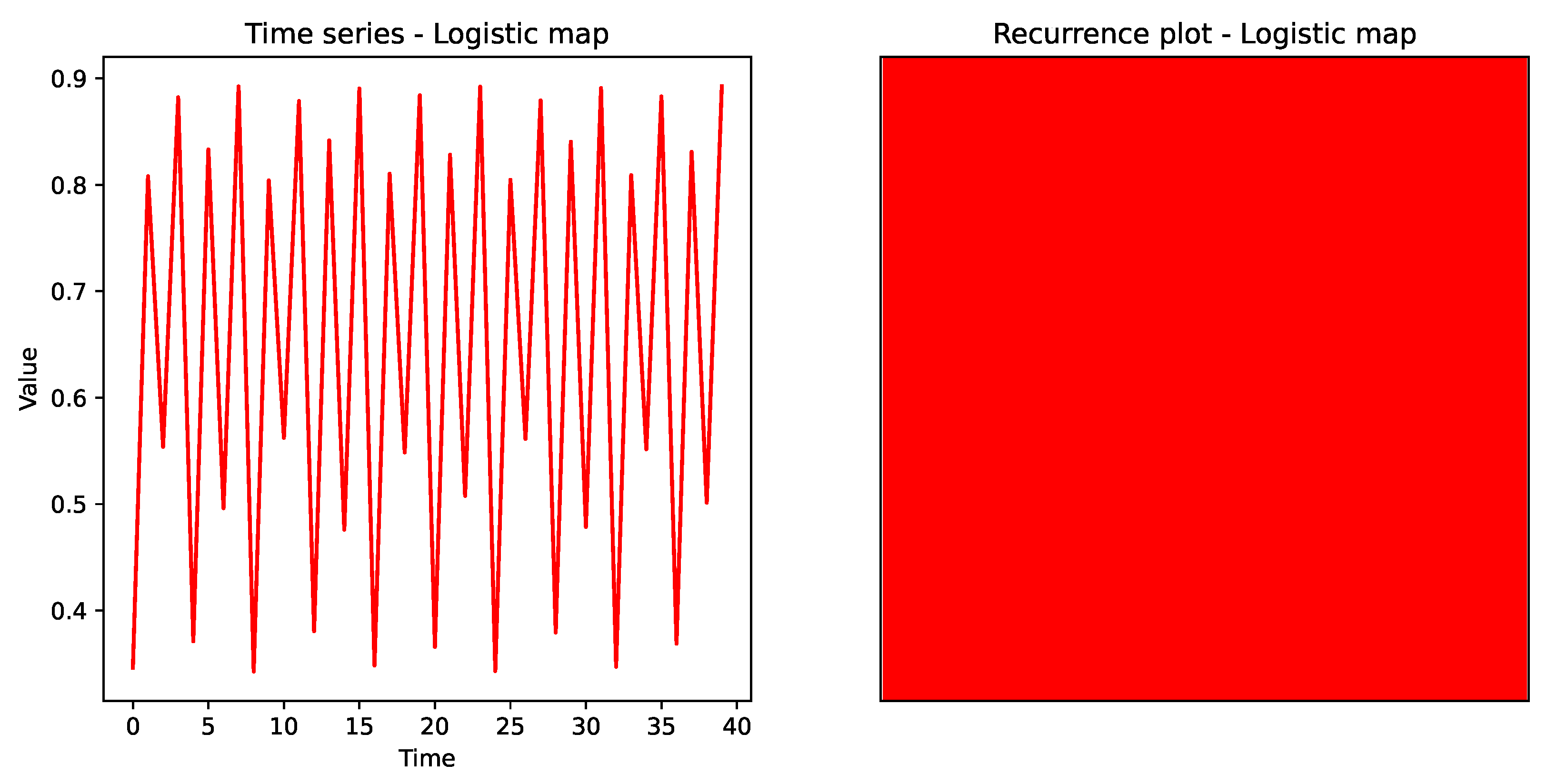
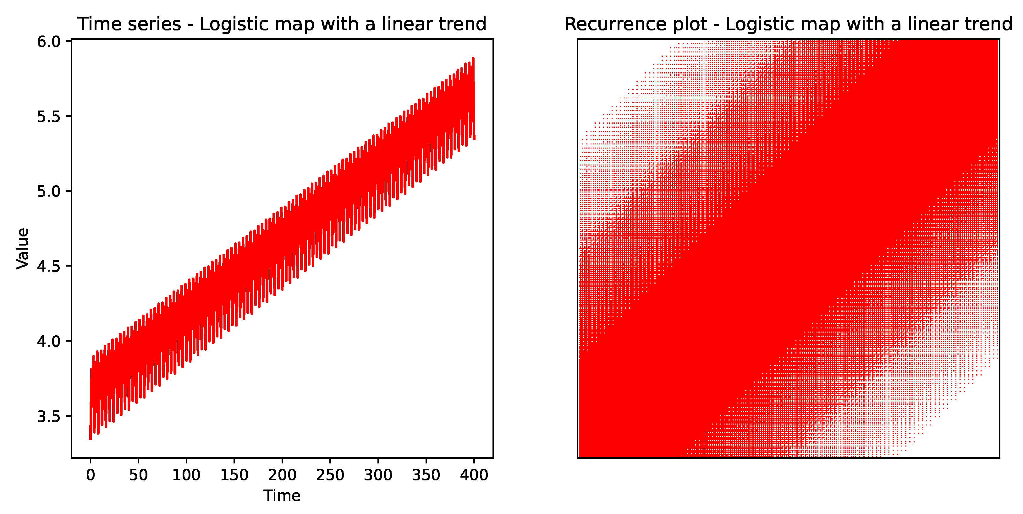
These benchmarking plots (
Figure 3,
Figure 4,
Figure 5,
Figure 6,
Figure 7 and
Figure 8) serve as reference classes for comparison with GNSS positioning errors and Dst-index results. Recurrence plots were created in this study using the Python programming language and the PyRQA library [
39]. The time series were generated using simulations of related processes in the R environment for statistical computing and the package fNonlinear [
31,
40]. Example classes of time series include the recurrence plots for a sine function, white noise (a normal Gaussian distribution), an AR system, Brownian motion, and a logistic map [
41]. The recurrence plots were qualitatively analysed based on their visual patterns. Homogeneous plots suggest stability, diagonal lines indicate deterministic behaviour, and vertical lines signal periods of stasis or slow change [
38], as visible from the quantitative analysis of the RPA results listed in
Table 3.
Recurrence plots with periodic diagonal lines are typical for oscillating systems. The distance between the diagonal lines reveals the oscillation period.
Figure 3 represents an oscillator (periodic oscillatory behaviour) on the example of a sine function, where the recurrence variables
,
,
,
L,
,
and
were
,
, 227622,
,
,
,
, and
, respectively.
Fading patterns indicate non-stationary behaviour in the underlying time series, such as the auto-regressive time series in
Figure 4, which has a negative correlation of
and a standard deviation of
. For the auto-regressive time series, the recurrence variables
,
,
,
L,
,
,
, and
were
,
, 41643,
,
,
,
, and
, respectively.
Systems with a drift tend to fade towards the upper-left and lower-right corners. An example of such a system is the Brownian motion depicted in
Figure 5, which was generated artificially using a dedicated R script. For the Brownian motion, the recurrence variables
,
,
,
L,
,
,
, and
were
,
, 24052,
,
,
,
, and
, respectively.
White disrupted areas are indicative of abrupt transitions in the system dynamics. For the white noise in
Figure 6, the recurrence variables
,
,
,
L,
,
,
, and
were
,
, 253132,
,
,
,
, and
, respectively. Clear borderlines within a recurrence plot represent chaotic transitions. Plots containing single recurrence points represent systems with fluctuation, containing states that are rare.
The states that evolve similarly at different times generate diagonal lines. These are indicative of deterministic processes. Vertical lines in a recurrence plot are present when there are states that remain the same for a certain time or that change very slowly. The logistic map in
Figure 7, defined as
at the onset of chaos with the parameter R set to
and
, exhibited high predictability in the last 400 points after 1000 data points were generated. The recurrence variables
,
,
,
L,
,
,
, and
for the logistic map were 1, 1, 1200,
,
,
, 1, and 401, respectively.
The addition of a linear trend (
) significantly alters the appearance of the logistic map in
Figure 8 when compared to the purely chaotic logistic map in
Figure 7, even though the parameter R and starting value
were set to the same values, and the same number of points was generated. The recurrence variables
,
,
,
L,
,
,
, and
for the logistic map with a linear trend were
,
, 6679,
,
,
,
, and
, respectively. As this does not represent the typical case for a logistic map, this example is purely illustrative and was not compared to the horizontal positioning errors or Dst-index data.
The visual appearance of a recurrence plot [
30] gives hints about the dynamics of the system. Caused by the characteristic behaviour of the phase space trajectory, a recurrence plot contains typical small-scale structures, such as single dots, diagonal lines, and vertical/horizontal lines (or a combination of the latter, which form extended clusters). The large-scale structure, also called texture, can be visually characterised as homogeneous, periodic, drift or disrupted. For example, the plot can show that if the trajectory is strictly periodic with a period
T, then all such pairs of times will be separated by a multiple of
T and will be visible as diagonal lines.
Typical examples of recurrence plots [
30,
31] have been examined in this paper, with a time series plotted over time and corresponding recurrence plots. These classes of recurrence plots include harmonic oscillation with a single frequency in
Figure 3, data from an auto-regressive process in
Figure 4, Brownian motion in
Figure 5, uncorrelated stochastic data (Gaussian white noise) in
Figure 6, chaotic data (a logistic map) in
Figure 7, and chaotic data (a logistic map) with a linear trend in
Figure 8.
The small-scale structures in recurrence plots contain information about specific characteristics of the underlying system’s dynamics. For example, the length of the diagonal lines visible in the recurrence plot is related to the divergence of phase space trajectories. Thus, it can represent information about the chaoticity [
27]. Therefore, the recurrence quantification analysis quantifies the distribution of these small-scale structures [
42,
43,
44]. This quantification can be used to describe the recurrence plots in a quantitative way. Applications include classification, predictions, nonlinear parameter estimation, and transition analysis. In contrast to the heuristic approach of the recurrence quantification analysis, which depends on the choice of the embedding parameters, some dynamical invariants, such as correlation dimension,
entropy or mutual information, which are independent of the embedding, can also be derived from recurrence plots. The base for these dynamical invariants is the recurrence rate and the distribution of the lengths of the diagonal lines [
27]. More recent applications use recurrence plots as a tool for time series imaging in machine learning approaches and studying spatio-temporal recurrences [
45]. Close returns plots are similar to recurrence plots. The difference is that the relative time between recurrences is used for the
y-axis (instead of absolute time) [
44]. The main advantage of recurrence plots [
30] is that they provide useful information even for short and non-stationary data, where other methods fail.
3. Results
The RPA results for the horizontal positioning errors [m] in 2014, separated by month, are presented in
Table 4. The lowest value for each variable is underlined and bold, and the highest value is bold. The lowest values for the
,
,
L,
,
, and
variables occurred in March, specifically
,
,
,
,
, and
, respectively. The highest values for the
,
,
L,
,
, and
variables occurred in June, equal to
,
,
,
,
, and
, respectively. The lowest value of
for the
variable occurred in April. The highest value for the
variable occurred in July, equal to
. The highest value of
for the
variable occurred in October, and the lowest value of
occurred in January, May, June, July, and August.
Key observations for quiet months such as June and July suggest that the recurrence plots resemble the sine class, with higher recurrence rate () and entropy values, indicating more stable ionospheric conditions. In disturbed months, such as March, April, and September, recurrence plots shift towards autoregressive or Brownian classes, with reduced line density and lower RPA parameter values, consistent with abrupt ionospheric transitions. Monthly variations in trapping time () and laminarity () peak during quiet months, showing that states persist longer under stable ionospheric conditions.
The RPA results for the Dst-indices [nT] in 2014, separated by month, are presented in
Table 5. The lowest value for each variable is underlined and bold, and the highest value in each row is bold. The lowest values for the
and
variables occurred in February, specifically
and 1109382, respectively. The highest values for the
and
variables occurred in July, with values of
and 3160916, respectively. However, all month had a
of
and a
of 1. The lowest values for the
L and
variables occurred in December, specifically
and
, respectively. The highest values for the
L and
variables occurred in October, with values of
and
, respectively. The lowest value for the
variable was
, which occurred in October. The highest value of
for the
variable and
for the
variable occurred in February. The lowest value of
for the
variable occurred in July.
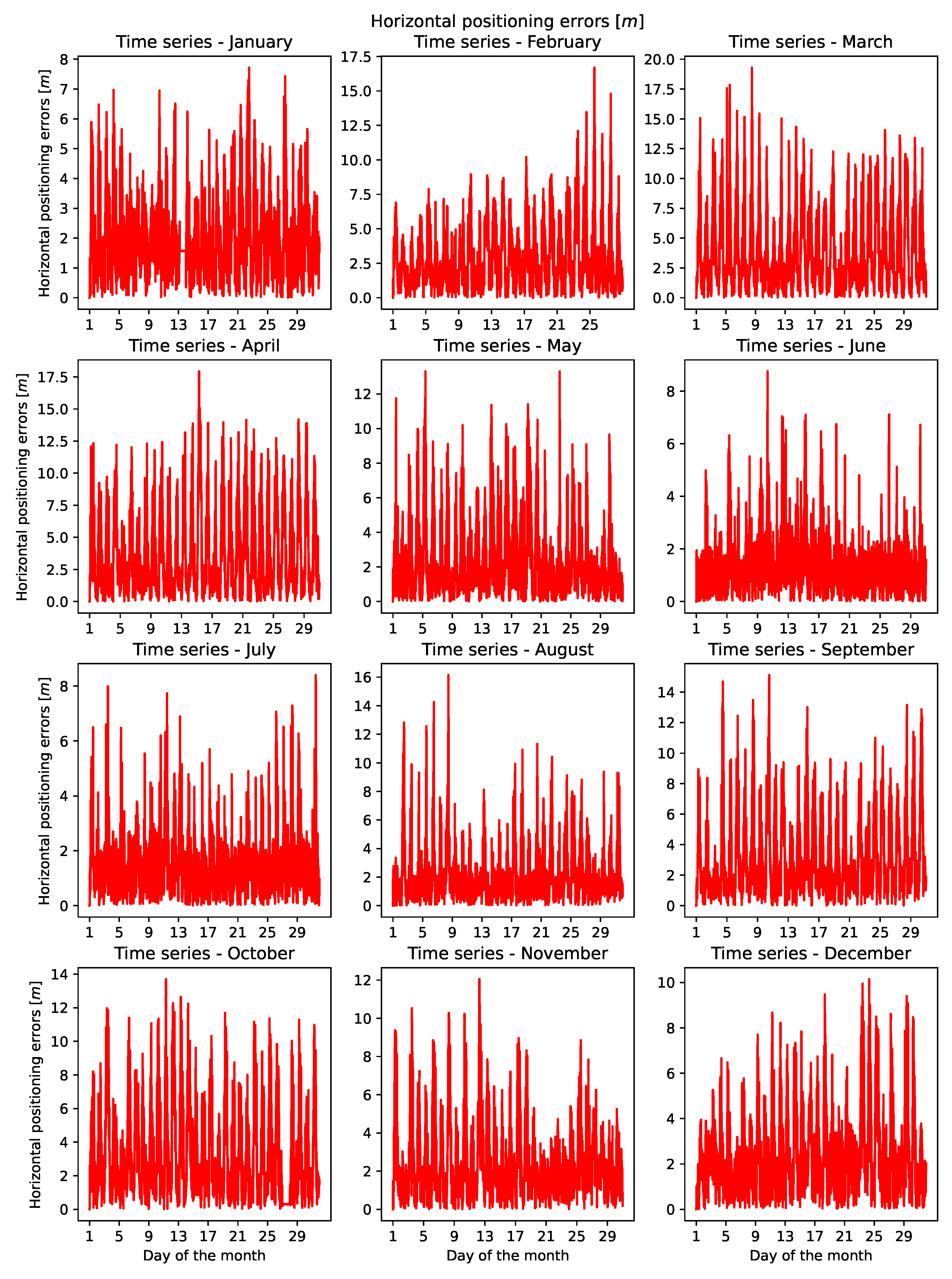
Figure 9 presents the time series of horizontal errors, while
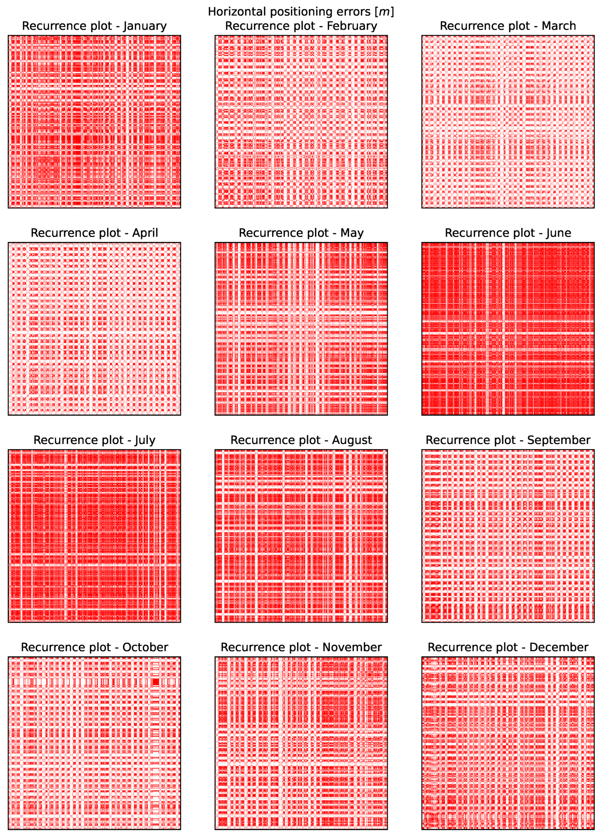
Figure 10 shows their recurrence plots by month.
To provide context for GNSS errors, we analysed monthly Dst-index time series with RPA. Results are provided in
Table 5. Across all months, recurrence plots for Dst resemble AR processes, consistent with geomagnetic storm dynamics. Stronger storms (low Dst) overlap with outlier horizontal positioning errors, confirming coupling between geomagnetic disturbances and ionospheric delay effects. The lowest entropy and highest trapping times occurred in October, consistent with extended geomagnetic storm activity.
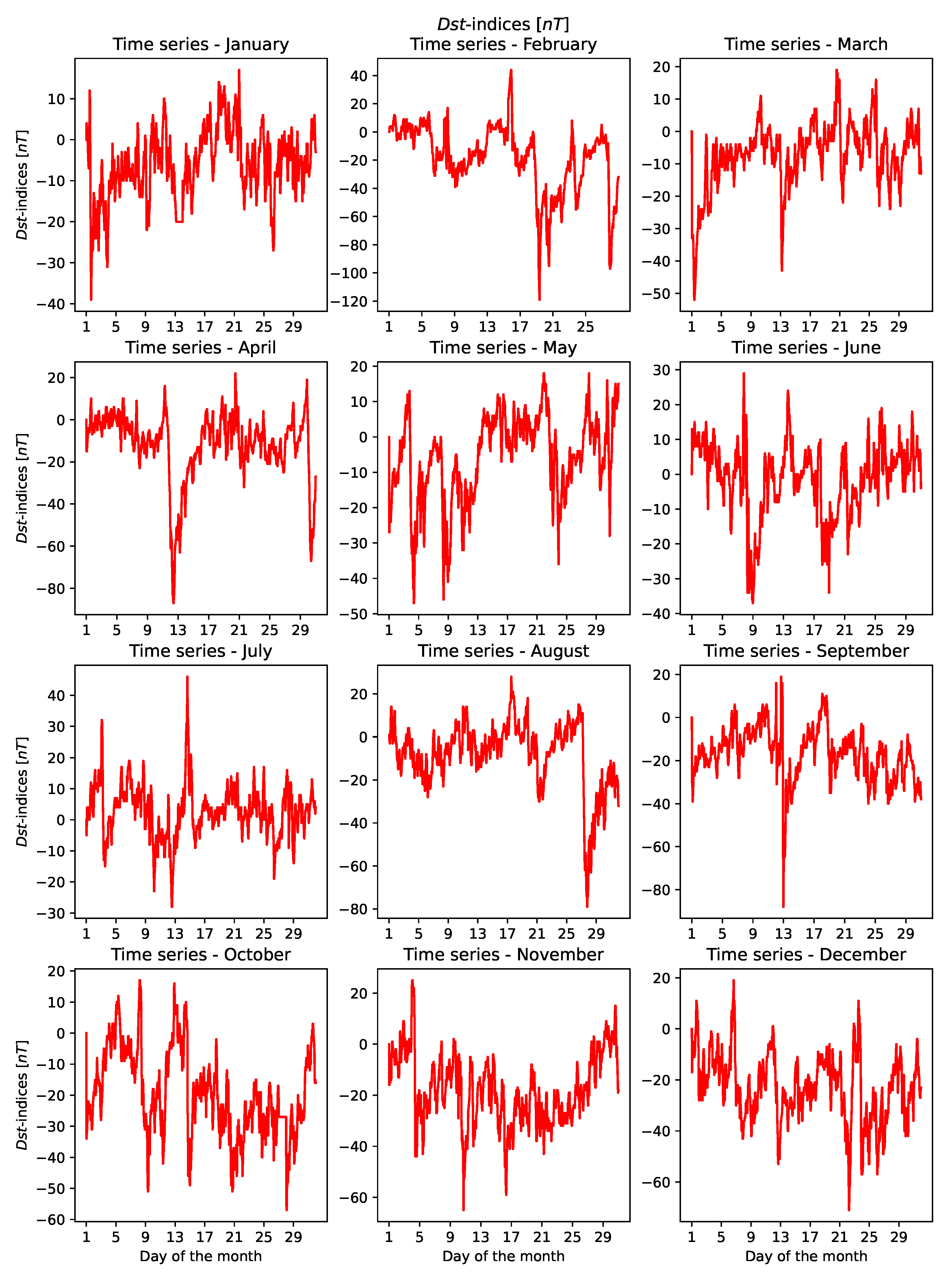
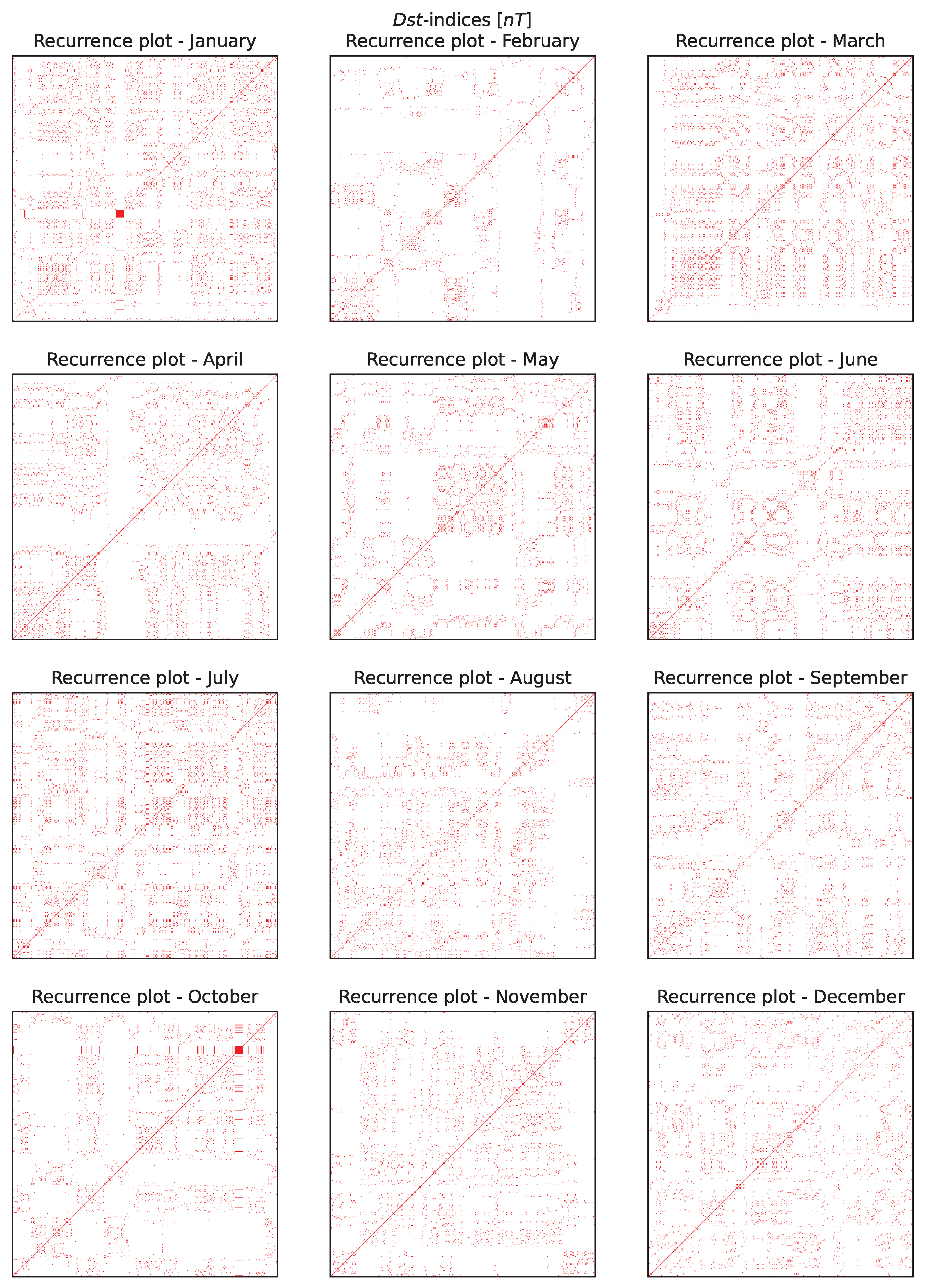
Figure 11 and
Figure 12 illustrate the monthly time series and recurrence plots for the Dst-index, respectively.
To interpret GNSS error results, we compared recurrence plots with well-known classes of time series, including sine functions, Gaussian noise, Brownian motion, auto-regressive processes, and logistic maps. This benchmarking allows us to associate GNSS behaviours with standard nonlinear dynamics. The RPA results for the horizontal positioning errors [m] in 2014, separated by month, and compared to the baseline functions by the absolute value of the difference in
(
) are presented in
Table 6. The name and value are listed for the baseline function with the lowest absolute value of the difference in
for each month (
). June and July have the lowest absolute value of the difference in
when compared with the sine class of recurrence plots because they also have the two largest
values among all the months when viewed separately. January and August have the lowest absolute value of the difference in
when compared with the normal (white-noise) class of recurrence plots because they also have the fourth-largest and third-largest
values, respectively. March and April have the lowest absolute value of the difference in
when compared with the auto-regressive class of recurrence plots, as they also have the two lowest
values among all months when viewed separately. All other months, February, May, and September through December, have the lowest absolute value of the difference in
when compared with the Brownian motion class of recurrence plots.
To directly compare GNSS positioning errors with benchmark functions, we computed the absolute difference in recurrence rate (
) between observed GNSS error plots and each baseline function. The results in
Table 6 show that June and July most closely resemble the sine function (low
), consistent with regular error patterns under quiet ionospheric conditions. March and April resemble AR processes, indicating disturbed, autoregressive-like dynamics. Other months tend to resemble Brownian motion or white noise, showing stochasticity under intermediate conditions.
The RPA results for the Dst-indices [nT] in 2014, separated by month, and compared to the baseline functions by the absolute value of the difference in
(
) are presented in
Table 7. The name and value are listed for the baseline function with the lowest absolute value of the difference in
for each month (
). All the months have the lowest absolute value of the difference in
when compared with the auto-regressive class of recurrence plots.
The time series plots for the horizontal positioning errors [m] in 2014, separated by month, are presented in
Figure 9. The time series and recurrence plots for the horizontal positioning errors [m] and Dst-indices [nT] in January, June, July, and August, shown in
Figure 9,
Figure 10,
Figure 11 and
Figure 12, consistently display lower values for the horizontal positioning errors [m] in the time series data in
Figure 9 and a large number of vertical lines in the recurrence plot in
Figure 10, paired with higher values for the Dst-indices [nT] in the time-series data in
Figure 11. This aligns with the high values for the RPA variables for the horizontal error in
Table 4 and for the Dst-index in
Table 5, indicating that states remain constant for a certain period or change very slowly.
The recurrence plots for the horizontal positioning errors [m] in 2014, separated by month, are presented in
Figure 10. The recurrence plots in
Figure 10 for the horizontal positioning errors [m] in June and July resemble the sine class of recurrence plots. The recurrence plots in
Figure 10 for the horizontal positioning errors [m] in January and August resemble the normal (white-noise) class of recurrence plots.
The time series plots for the Dst-indices [nT] in 2014, separated by month, are presented in
Figure 11. The time series and recurrence plots for the horizontal positioning errors [m] and Dst-indices [nT] in February through May and September through December, shown in
Figure 9,
Figure 10,
Figure 11 and
Figure 12, reveal high outlier values in the time series data for the horizontal positioning errors [m] in
Figure 9 and a small number of vertical lines in the recurrence plot in
Figure 10. The outliers with high values in the horizontal error time series in
Figure 9 coincide with extremely low values in the Dst-index time series in
Figure 11. This aligns with the low values for the RPA variables for the horizontal error in
Table 4 and for the Dst-index in
Table 5, indicating abrupt transitions in the system dynamics.
The recurrence plots for the Dst-indices [nT] in 2014, separated by month, are presented in
Figure 12. The recurrence plots in
Figure 10 for the horizontal positioning errors [m] in February through May, and September through December, and the recurrence plots in
Figure 12 for the Dst-indices [nT] in all months, resemble the auto-regressive class of recurrence plots.
All the plots, separated by month, reveal a combined tendency of recurrence plots in
Figure 10 that generally resemble those of a normal Gaussian distribution or a sine function for the horizontal error time series in
Figure 9. The recurrence plots in
Figure 12 resemble an auto-regressive function for the Dst-index time series in
Figure 11.
During geomagnetically quiet months, recurrence plots of GNSS horizontal errors closely resembled periodic oscillatory systems (sine class), with high recurrence rate (), entropy (), and trapping time (). These features indicate stability in error dynamics under relatively undisturbed ionospheric conditions. In contrast, disturbed months showed patterns resembling autoregressive or Brownian processes, consistent with abrupt transitions and stochastic fluctuations induced by ionospheric storms.
The Dst-index, by comparison, consistently exhibited autoregressive-like recurrence structures, reflecting the gradual buildup and decay of geomagnetic storms. Importantly, months with strongly negative Dst values coincided with reduced RPA variables in GNSS error plots, confirming the coupling between geomagnetic activity and positioning degradation. Strong geomagnetic storms (low Dst) systematically coincided with higher GNSS positioning errors, strengthening the case for using recurrence variables as early indicators of performance degradation.
4. Discussion
In this work, we used RPA to examine the nonlinear dynamics of GPS horizontal positioning errors in a sub-equatorial region, cross-referencing our findings with the geomagnetic Dst-index. The analysis showed a clear systematic variation in the recurrence structures of GNSS errors, depending on whether the geomagnetic environment was quiet or disturbed.
Our benchmark tests using canonical time series such as sine functions and Brownian motion established a robust guideline for interpreting the complex dynamics observed in GNSS errors. A key finding was the distinction between quiet and disturbed periods. During quiet months, horizontal errors showed structured, periodic recurrence patterns, while in disturbed months, their dynamics shifted toward stochastic, autoregressive-like behaviour.
The consistent autoregressive-like structure of the Dst-index confirmed its strong negative correlation with GNSS performance, where low Dst values consistently corresponded to higher positioning errors. This analysis highlighted that RPA variables like recurrence rate, entropy, and trapping time are valuable nonlinear indicators of performance degradation, providing potential new frontiers beyond traditional statistical measures.
The urban relevance of the study is increased since we employed a single-frequency, commercial-grade receiver, representative of smartphones, IoT devices, and consumer-grade navigation, and the findings are directly applicable to urban mobility, smart city services, and resilient GNSS applications.
Limitations of this work include its focus on a single GNSS station and exclusion of the vertical positioning component. Nevertheless, these choices were deliberate to highlight horizontal accuracy, which is critical for urban services.
Future work will extend the analysis to multiple stations across diverse latitudes, multi-constellation GNSS observations (Galileo, BeiDou, GLONASS), and vertical positioning errors, which are particularly sensitive to ionospheric conditions.
By demonstrating the utility of RPA in detecting and characterising GNSS error dynamics, this study contributes to both the field of space weather monitoring and the design of resilient GNSS systems for urban applications.
Our results demonstrate that the recurrence plots of horizontal positioning errors during specific months of the year align well with established nonlinear models, particularly those for white noise in
Figure 6, and sine functions. This alignment provides a foundation for developing more accurate models for GNSS pseudorange and position estimation errors.
The Dst-index consistently produced recurrence plots characteristic of an autoregressive process, confirming its predictable, decaying nature following a disturbance. In contrast, the horizontal error time series exhibited more varied dynamics, resembling either a periodic system (like a sine function) during quiet months or a stochastic one (like white noise) during disturbed periods.
In several months, the horizontal positioning error exhibited recurrence structures resembling white noise. The resemblance of some error structures to white noise does not suggest a lack of connection to geomagnetic processes, but rather points to the highly stochastic nature of ionospheric variability. In this context, recurrence measures remain valuable, as they allow quantification of changes in stochastic behaviour using variables like entropy and recurrence rate to differentiate between quiet and disturbed conditions.
In periods such as February through May and September through December, outlier values increase the positioning errors, likely due to disturbed ionospheric conditions, observed in the Dst-index time series, which lower all RPA variables and move the distribution closer to an auto-regressive process. Most of the RPA variables, such as the recurrence rate, the Shannon information entropy of diagonal line lengths longer than the minimum ones, the total number of lines, and their average length in the recurrence plot, achieve their maximal values in months with lower horizontal positioning errors, without massive ionospheric disturbance events.
The fact warrants further research in terms of utilising GNSS positioning performance degradation forecasting and now-casting due to space weather, geomagnetic, and ionospheric disturbances. The horizontal positioning error time series tends to form more uniformly filled recurrence plots during quiet and modestly disturbed ionospheric conditions. Disturbed ionospheric conditions cause outlier values of large horizontal positioning errors, which in turn decrease the number of lines in the plot. A significant decrease in the total number of lines in the horizontal error recurrence plots is observed from February through May, as well as in September and December.
The presented study assesses the horizontal GPS/GNSS positioning error from the perspective of a single-frequency commercial-grade GPS receiver, thus focusing on the market prevailing class of GNSS receivers found in and utilised for a growing number of urban GNSS applications: location-based services, IoT devices, modern connected and autonomous road and aerial vehicles, as well as in Smart City devices, systems, and services [
10].
Identification of relevant long-term indicators of GNSS positioning performance for utilisation in the prevailing Software-Defined Radio GNSS receiver architectures, such as those implemented on smartphones and other devices, opens the room for development and operation of the
GNSS PNT in which the GNSS application may take an active role in mitigation of the GNSS ionospheric effects with the personalised correction models [
10]. The generic nature of the proposed
GNSS PNT should be noted, as it allows for its implementation in virtually every GNSS application empowered with ambient awareness and defined by its specific needs for GNSS positioning performance.
While this study employed the Dst-index, alternative indices such as (available at 1-min resolution) and the time derivative may provide even more sensitive measures of geomagnetic activity. is a proxy for induced electric fields (), which directly influence ionospheric plasma transport and could therefore impact GNSS positioning more strongly. Future work should extend the present recurrence analysis to these indices.
In addition, cross-recurrence plots (CRP) and joint recurrence plots (JRP) offer powerful methods to explicitly study the coupling between GNSS errors and space weather indices. Although our study focused on univariate recurrence as a first step, CRP and JRP represent a logical extension and will be considered in future research.
5. Conclusions
This study applied RPA to characterise time series patterns in GPS-derived pseudorange errors. Our results confirm that RPA is a powerful tool for characterising the nonlinear dynamics of GNSS errors. By identifying common classes of dynamical properties, this approach aims to improve the understanding and modelling of GNSS pseudorange errors and overall positioning performance, ultimately fostering the development of GNSS systems more resilient to ionospheric and space weather effects. We successfully demonstrated the utility of universal RPA methods for both GNSS pseudorange error and Dst-index time series. The analysis showed that during periods of strong geomagnetic activity, as indicated by low Dst values, the horizontal positioning errors exhibited stochastic, white-noise-like behaviour, whereas they displayed more predictable, periodic patterns during quiet periods.
This apparent randomness reflects ionospheric variability rather than the absence of a physical connection, and recurrence measures provide a way to characterise these stochastic transitions. The findings suggest that RPA variables like recurrence rate and trapping time can serve as novel indicators for predicting GNSS performance degradation and inform the development of more resilient navigation systems.
These prospects will be examined further and utilised in the design of GNSS user equipment and resilient GNSS developments in the forthcoming research activities. Research presented in this manuscript contributes to the subject as follows: (i) methodology development for studying the non-linear behaviour of GNSS horizontal positioning errors, as the major contributor to GNSS pseudorange measurement error and, hence, to GNSS positioning error, (ii) methodology development for studying the non-linear behaviour of horizontal positioning errors, as a widely accepted geomagnetic activity indicator, and Dst-indices, used to evaluate the intensity of ionospheric storms, and (iii) inference from the RPA that may advance understanding, description, and modelling the ionospheric effects on GNSS positioning performance.
The research results demonstrate the applicability of the developed GPS RPA methodology for assessing the nonlinear dynamics properties of the horizontal GPS positioning error, serving as a proof of principle. The presented research contributes to the development of the
GNSS PNT [
10], which is capable of active mitigation of the GNSS ionospheric effects in accordance with the real GNSS positioning, ambient conditions, and in compliance with the requirements for GNSS positioning performance of targeted GNSS applications.
Future research will address the long-term spatio-temporal properties of the non-linear dynamics of the horizontal GPS positioning errors through the assessment of data collected at selected IGS reference stations across the globe.
The research utilises single-station data to demonstrate a methodological framework for analysing nonlinear GNSS positioning errors, serving as a proof-of-principle in the characteristic scenario of the sub-equatorial region, known for its extreme ionospheric conditions. Further locations and date ranges will be included as the subject of further research. Future research will address the long-term spatiotemporal properties of horizontal GPS positioning errors by accessing and processing data collected from multiple IGS reference stations worldwide.
The authors are aware of more advanced positioning methods, such as Precise Point Positioning (PPP) and Real-time Kinematic Positioning (RTK). However, the authors address the Single Point Positioning (SPP) mode because it represents the predominant class of bulk, single-frequency receivers used in urban applications, such as smartphones, IoT devices, and consumer navigation. The purpose of the research is to understand and mitigate ionospheric effects on GNSS PNT, which supports many urban systems and services, rather than achieving the highest possible accuracy with more sophisticated and less common methods. Therefore, the SPP mode of operation is not trivial in the context of the research goals, as it represents the most relevant and targeted approach to solving real-world problems. Additionally, the presented research results can be applied to other advanced algorithms for GNSS PNT.
Such an approach would allow for classification of the GPS/GNSS utilisation scenarios and, consequently, more optimised modelling of the GPS positioning errors due to ionospheric effects for further enhancement of the GPS/GNSS resilience.
Features of the
GNSS PNT [
10] render it fit for implementation in various urban systems and services, thus allowing for significant performance improvement and raising the GNSS resilience against the natural and adversarial effects. In future studies, the use of higher-resolution indices, such as
, in conjunction with
, along with cross-recurrence and joint recurrence analysis, will provide deeper insights into the coupling between geomagnetic activity and GNSS errors.

