Article

Integrated Remote Sensing and Machine Learning for Urban Air Temperature Assessment and Mapping in Highly Heterogeneous Environments


by
Vahagn Muradyan
1,
Rima Avetisyan
1,
Shushanik Asmaryan
1,*,
Anahit Khlghatyan
1,
Azatuhi Hovsepyan
1,*,
Garegin Tepanosyan
1,
Andrea Bergamaschi
2 and
Fabio Dell’Acqua
2
1
Department of GIS and Remote Sensing, Center for Ecological-Noosphere Studies NAS RA, Yerevan 0025, Armenia
2
Department of Electrical, Computer, Biomedical Engineering, University of Pavia, 27100 Pavia, Italy
*
Authors to whom correspondence should be addressed.
Urban Sci. 2026, 10(5), 257; https://doi.org/10.3390/urbansci10050257
Submission received: 12 March 2026 / Revised: 26 April 2026 / Accepted: 30 April 2026 / Published: 8 May 2026
(This article belongs to the Section Urban Environment and Sustainability)

Abstract

This paper investigates the prediction of urban air temperature (Tair) from satellite-derived land surface temperature (LST) in the complex urban and topographic environment of Yerevan, Armenia. Building on previous work that demonstrated the effectiveness of machine learning (ML) approaches for point-based Tair estimation using Partial Least-Squares Regression (PLSR) with multiple environmental variables, this study shifts the focus to the spatial distribution of Tair. Several prediction methods and input variable combinations are evaluated to generate gridded Tair maps, which are assessed for spatial consistency against expected patterns driven by land cover, elevation, local knowledge, and spot observations. In total, five predicting methods were used—one regression approach (PLSR) and four ML methods: random forest (RF), quantile regression forest (QRF), support vector machine (SVM), multilayer perception (MLP). RF and QRF deliver the best overall results, with RF achieving the highest testing R2 (0.74) and lowest RMSE (0.56). Spatial patterns are similar for PLSR, RF and QRF, highlighting cooler northern high-altitude areas and warmer southern urban areas. Overall, the results confirm the reliability of the proposed Tair spatial mapping methods in complex urban environments.

1. Introduction

Air temperature (Tair), is an important atmospheric variable that directly reflects the energy budget of surface and the thermodynamic state of the boundary layer of the planet [1,2]. It is widely recognized as a primary metric for detecting and monitoring anthropogenically induced climate change, particularly within urban environments, where land use changes and anthropogenic heat emissions intensify local climate alterations [3,4].
The urban heat island (UHI) effect is directly determined by the Tair, which characterizes the elevated temperature in urban centers compared to surrounding rural areas. This phenomenon is the result of complex interactions between surface materials, geometry and human activity [5,6]. High-resolution spatial data on Tair are therefore crucial for accurately quantifying UHI intensity and understanding urban microclimate dynamics.
Despite its importance, in situ meteorological observations of Tair, typically recorded at 1.5 to 2 m above ground level—are limited by the sparse distribution of weather stations, especially within complex and heterogeneous urban landscapes [7,8]. The urban environment is defined by high spatial variability of surface characteristics, which leads to uneven sample coverage and significant gaps in observations in long-term climate records [9].
To address these limitations, satellite remote sensing provides a practical way of characterizing spatial patterns of urban thermal environment [10]. Although Tair cannot be directly obtained using space sensors, thermal infrared images (TIR) make it possible to assess the land surface temperature (LST), taking into account the emissivity of the surface and atmospheric effects. LST is strongly coupled with surface–atmosphere energy fluxes and serves as a proxy for near-surface Tair in many urban climatology studies [11]. This approach allows tracking both the seasonal behavior and the fine-scale spatial distribution of Tair.
This study investigates these dynamics in the context of Yerevan, Armenia, a medium-sized city located in a complex topographic environment. Yerevan covers an area of approximately 220 km2, but within its urban extent there is a difference in elevation of more than 500 m (Yerevan Green City Action Plan. Available online: https://www.yerevan.am/en/yerevan-green-city-action-plan, accessed on 29 April 2026). The city experiences a semi-arid continental climate and is served by only three operational public weather stations, severely constraining the spatial resolution of traditional observational datasets. The combination of rugged hypsometry, limited spatial extent, and sparse ground-based monitoring presents a unique case for evaluating remote sensing-based methods of Tair estimation and for advancing our understanding of urban thermal regimes in complex mountainous regions. Hence, the aim of this study is to answer the following scientific questions:
  • Is it feasible to estimate Tair in a city with a complex elevation pattern, such as Yerevan, based on a given set of environmental variables?
  • Independently of the accuracy of the individual temperature estimates mentioned above, is it possible in such a context to provide a meaningful spatial distribution of temperatures across the urban area based on the same variables?

1.1. State of the Art (SoA)

This section reviews the current state of the art in urban Tair assessment and mapping in complex and varied urban landscapes. The following sections will provide overview of mythologies, applications, and remaining challenges associated with using these data sources to comprehensively understand and hopefully mitigate the effects of urban overheating.

1.1.1. Remote Sensing for Temperature Mapping

Traditional weather stations have notable limitations when it comes to spatially predicting and mapping Tair. Remote sensing data provides an effective alternative: although Tair cannot be measured directly from space, thermal infrared sensors enable the derivation of land surface temperature (LST). It is important to note that variables Tair and LST are physically different: Tair represents shaded near-surface Tair measured at standard height, whereas LST is the radiometric skin temperature of heterogeneous urban surfaces [12]. Despite this non-equivalence, LST has been shown to be an effective statistical predictor of Tair when combined with additional environmental variables․ LST is fundamental to the energy balance and serves as a widely used proxy for estimating the spatial distribution of Tair [13,14]. This approach facilitates the study of both seasonal trends and small-scale thermal heterogeneity in urban areas. Land Surface Temperature (LST) is, in fact, widely considered the most relevant satellite predictor for Tair estimation [14,15,16,17,18,19,20,21]. Approaches utilizing LST include the Temperature-Vegetation Index (TVX), which assumes cooler temperatures in vegetated areas. While the surface temperature of a dense vegetation canopy can closely mirror Tair in theory, this method is unsuitable for urban Tair retrieval, which must focus on the temperature relationship over unvegetated and built-up surfaces [22,23]. Energy balance approaches also use LST along with other thermodynamic variables, but they often require inputs not directly measured by satellites [15,19].

1.1.2. Statistical Techniques and Their Applicability

Statistical techniques for Tair prediction generally involve spatial interpolation methods or regression methods. Spatial interpolation, including both deterministic (e.g., Inverse Distance Weighting, polynomial functions) and stochastic (e.g., kriging-based, Geographic Weighted Regression) methods [17,24,25,26] works effectively when weather stations are well-distributed and predictions are made at the same time as model generation. However, for long-term daily observations or areas with irregular weather station coverage, such as our study area of Yerevan, these methods lose accuracy [13,20,26,27]. Therefore, spatial interpolation is not a viable approach for accurate Tair prediction in Yerevan.
This leads us to regression methods that are suitable in cases where interpolation is ineffective. They range from parametric models such as Linear regression (LR) and Stepwise Regression [19,28,29,30,31,32] to more complex ML methods such as RF, SVM an NN [19,31,33]. These empirical regression models use training and testing processes to develop optimal estimate of Tair, even in areas with highly heterogeneous landscape characteristics.

1.1.3. Unique Challenges in Mountainous Urban Environments

Our study focuses on Yerevan, Armenia, a city presenting unique geographical parameters and a distinct challenge compared to typical urban heat island studies. While other case studies have used remote sensing for Tair prediction (such as Athens, Heraklion, Los Angeles, Seoul, Vancouver, and Erbil [33,34,35] (Yerevan combines a complex mountainous terrain with a relatively small area (approximately 220 sq km), exhibiting an absolute elevation variation exceeding 500 m (over 1600 feet). Adding to this complexity, Yerevan has a dry climate and only three operational weather stations, severely limiting the available information on Tair’s spatial variation.

1.1.4. Hybrid Methodologies and Machine Learning for Urban Tair Modeling

Remote sensing-based (RS-based) Tair estimation often employs a hybrid methodology that combines Geographic Information System (GIS) and remote sensing data. For instance, Cristobel et al. (2008) integrated spatial variables (e.g., altitude, latitude, continentality, solar radiation) with RS predictors like albedo, LST, and NDVI, finding this combined approach underpins the best Tair models, with NDVI and LST being the most powerful RS-based predictors [36]. It is crucial to acknowledge that while LST is a fundamental physical parameter strongly related to near-surface Tair, their relationship becomes more intricate in mountainous areas or where weather station availability is limited. Nonetheless, Mutiibwa et al. (2020) found a consistent relationship between LST and Tair even in complex mountainous regions of Nevada [37]. Interestingly, Nikoloudakis et al. (2020) developed RS-GIS-based methodology to predict Tair in cities without LST relying on the morphological features of the cities and on-site measurements [35].
Modeling urban Tair is inherently complicated due to urban heterogeneity, where sparse weather stations hinder accurate spatial representation [38], and this is further compounded in mountainous urban areas [33]. Fortunately, ML techniques significantly improve the accuracy of Tair estimations [39]. While multiple regression and Artificial Neural Networks (ANN) models remain popular [28,38,39,40,41], with varying results often due to input variable selection, the strength of ML models lies in their ability to handle numerous variables. In this study, we utilized regression PLSR, QRF, RF, SVM, and MLP ML models to assess and predict urban Tair, incorporating 31 different variables: these consist of 15 environmental variables (Section 2.3.1), for which both the mean and standard deviation were calculated within each 1 km × 1 km grid cell, an additional temporal variable, Day of Year (DOY), was included, yielding a total of 31 predictors. We specifically selected the RF model as our regressor for estimating spatial hourly Tair patterns because it not only offers superior advantages but also allows us to assess the importance of each driver to the estimation accuracy [42], which is vital for this research. Beyond overall and temporal performance, we also meticulously examined how these models performed across different spatial locations.

2. Materials and Methods

2.1. Study Area

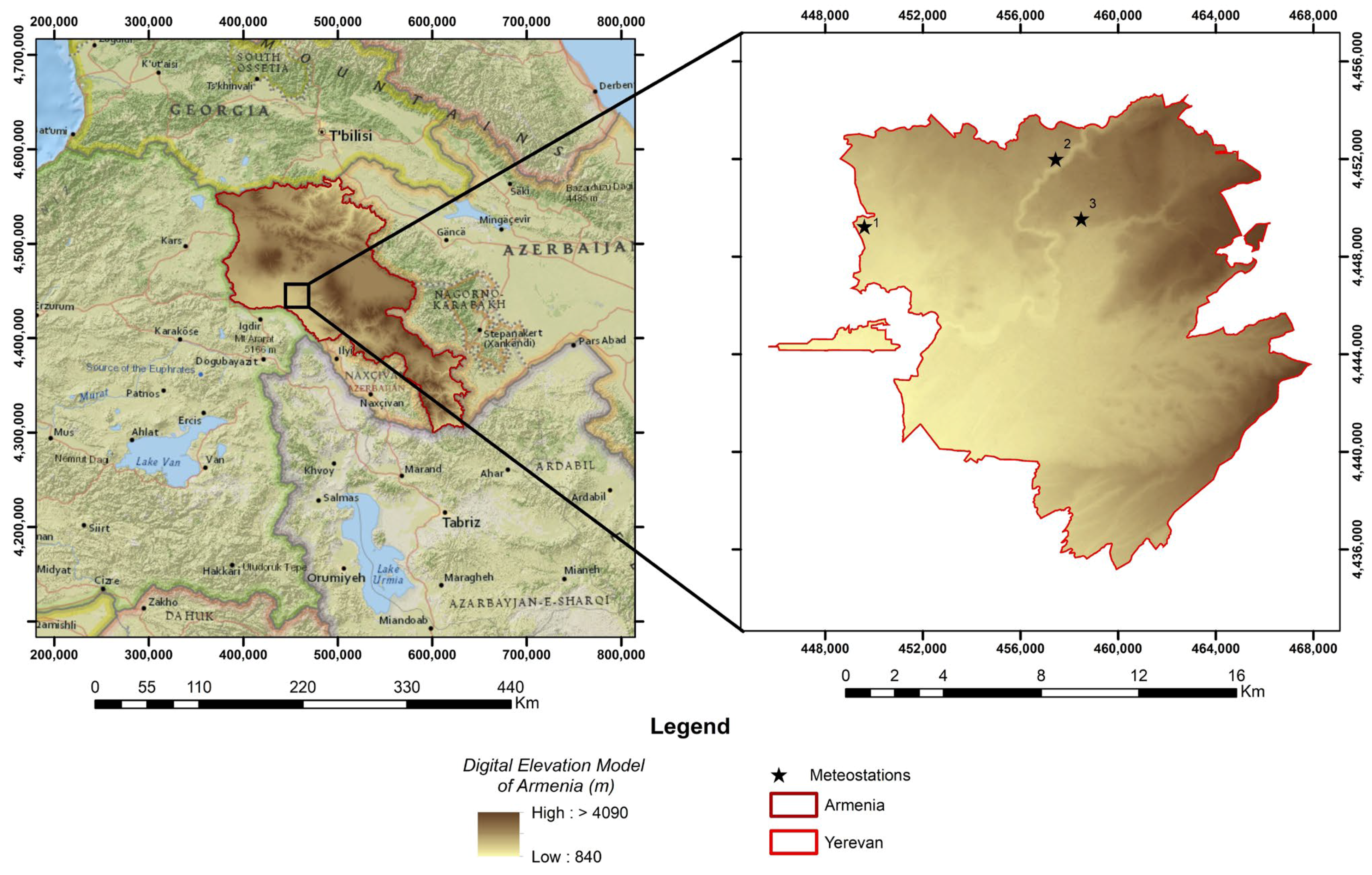
Yerevan is the capital of Armenia, with a sprawling urban center covering approximately 223 km2 and home to 1.1 million inhabitants. It is defined with the significant concentration of population of Armenia—36% of the total and the 56% of its urban residents. The population density of Yerevan is quite high, exceeding 4900 inhabitants/km2 (https://www.armstat.am/en/ (accessed on 29 April 2026)). Geographically, Yerevan is situated on a plain at the edge of the Ararat Valley, with elevations ranging significantly from 850 m to 1400 m (Figure 1), showcasing its mountainous character (https://www.yerevan.am/en/yerevan-green-city-action-plan (accessed on 29 April 2026)). The city has dry continental climate with an average annual Tair between 9.1 °C to 12.1 °C. This leads to significant seasonal fluctuations, with the 27 °C difference between summer and winter temperatures.
Winters here are particularly cold and snowy, with average January temperatures ranging from −2.5 °C to −5 °C, and absolute minimum reaching −21 °C to −32 °C. Springs are brief and volatile. Summers are long, hot and dry, with average Tair ranging from 22.1 °C to 25.4 °C. The absolute maximum Tair recorded in July can climb to between 40 °C and 43 °C [26,27].
Located in a dry subtropical climate zone, Yerevan is particularly susceptible to climate change, which is evident in the increasing amplitude of urban Tair swings.
Figure 1 visually depicts Yerevan’s geographical allocation, in the country revealing both its mountainous topography and, crucially, the sparce distribution of weather stations. These stations are predominantly located in the city’s north and west at varying altitudes (Figure 1), severely limiting our ability to observe the spatial variations in Tair across the entire urban area.
Since the late 1980s, rapid land cover changes in Yerevan have intensified the city’s exposure to recent climate shifts. A national communication on climate change reveals a striking increase of approximately 40 days, on average, in Yerevan’s summer heatwave period between 1981 and 2013 (https://nature-ic.am/en; https://unfccc.int/resource/docs/natc/armnc3.pdf (accessed on 29 April 2026)). While some research, such as Tepanosyan et al.’s study, has investigated the influence of spatio-temporal land cover changes on surface urban heat using remote sensing data (Landsat TM/ETM+/OLI-TIRS images) [43], no previous studies have specifically addressed the development of methods to improve the visualization and monitoring of spatio-temporal Tair variations using remote sensing data and techniques specifically for this area.

2.2. Input Data

2.2.1. Ground-Based Data

Meteorological data were sourced from three weather stations located within or near Yerevan. Data was provided by the “Hydrometeorology and Monitoring Center” State Non-Commercial Organization (SNCO) of Ministry of Environment of Republic of Armenia. Stations are equipped with a comprehensive set of “MicroStep-MIS” instruments, providing both daily and hourly measurements across a wide range of meteorological parameters. These parameters include horizontal visibility, cloudiness, atmospheric phenomena, surface and subsurface soil temperature, Tair, relative humidity, atmospheric pressure, wind direction and speed, precipitation, sunshine duration, dew point and solar radiation. For this study, our analysis specifically focused on Tair. For this study, Tair data were aggregated to daily averages corresponding to the local time of satellite overpass, ensuring alignment between in situ measurements and remotely sensed LST for model training.
Before analysis, raw data was meticulously processed. Initially, all measurements were considered, followed by a crucial step to identify and remove outliers. The boxplot method was used to identify potential outliers, with values outside the range Quartile 1 (−1.5× interquartile range) and Quartile 3 (+1.5× interquartile range) marked accordingly. However, to ensure data integrity, only data points identified as outliers across all measured parameters were ultimately excluded. Observations that were flagged as outliers in only some of the parameters were retained, minimizing the removal of potentially valid data and ensuring that only true anomalies were discarded.

2.2.2. Remote Sensing Data and Topographic Information

The analysis relied on a comprehensive input dataset of open-source remote sensing (RS) surface reflectance products from Landsat missions, specifically Landsat 4 and Thematic Mapper (TM), Landsat 7 Enhanced Thematic Mapper Plus (ETM+), and Landsat 8 Operational Land Imager/Thermal Infrared Sensor (OLI/TIRS). These images monitor the summer season (June to August) spanning from 1984 to 2020 and were acquired and processed using Google Earth Engine (GEE) platform.
To enrich this dataset, several key spectral indices were computed, including Normalized Difference Vegetation Index (NDVI), Normalized Difference Water Index (NDWI), the Index-Based Build-Up Index (IBI) and the Soil-Adjusted Vegetation Index (SAVI).
Furthermore, Land Surface Temperature (LST) for each year was derived using the Landsat LST Web Application, which provides data with a spatial resolution resampled to 30 m. In addition to these remote sensing products, topographic variables such as elevation, aspect, slope, and solar radiation were incorporated along with the Terrain Ruggedness Index [44]. These topographic variables were all derived from a 30 m digital elevation model (DEM), based on Shuttle Radar Topography Mission—SRTM (https://dwtkns.com).
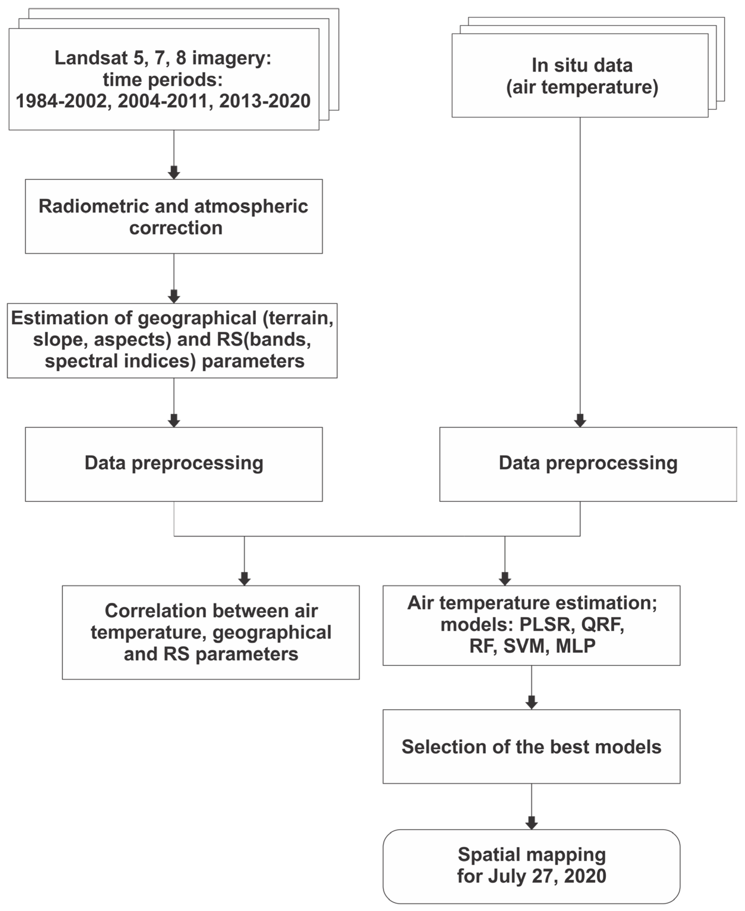
In addition to natural and topographic factors, two variables, LST and the IBI, were included to represent anthropogenic influences. LST reflects the combined effects of surface materials and human heat emissions, while IBI quantifies urbanization intensity and impervious surface coverage, both of which are key determinants of elevated urban Tairs. Figure 2 illustrates the detailed steps undertaken in this study.

2.3. Methods and Algorithms

2.3.1. Statistical Analyses and ML Modeling

To model and predict Tair distribution across Yerevan, various machine learning techniques were employed. The methods were selected due to their ability to effectively catch dependencies between input features and the response variable—Tair. A combination of traditional regression methods and more advanced ML algorithm were applied to enhance prediction accuracy.
All statistical analyses were performed using the Python (v3.13.9) coding in the Jupiter Notebook environment. The task of Tair prediction and mapping was framed as a supervised regression problem. This research selected one statistical approach, Partial Least-Squares Regression (PLSR), and four more advanced non-parametric machine learning algorithms for evaluation: Support Vector Machines (SVM), Multilayer Perceptron (MLP), Random Forests (RF), and Quantile Regression Forest (QRF) [19,33,45].
To estimate and map Tair in Yerevan, using these ML models, various meteorological, satellite and environmental data were used as input variables. In Section 2.3.1, the complete list of 31 input variables are presented, including spectral, thermal, topographic and thermal factors with their importance to urban air (Tair) assessment. The variables include satellite-derived spectral bands such as blue, green, red, near infrared (NIR), shortwave infrared 1 (SWIR1) and shortwave infrared 2 (SWIR2). In addition, several derived indices were included: NDVI, NDWI, IBI and SAVI. To capture surface heat characteristics, LST was included as a key variable. Among geographical factors, the list of some input variables were also included, recognized as significant microclimatic drivers, such as slope, elevation, terrain roughness and solar radiation.
Tree complementary importance indicators were applied to interpret the contribution of variables in different models. For PLSR indicators of importance of variables in the projection (VIP) were calculated, with values ≥ 1 indicating significant predictors. For RF the importance of features was assessed using both the average decrease in impurity (Gini importance) across all trees and the importance of permutations on the test set, which provided a more reliable estimate that was less susceptible to bias towards features with high cardinality. For QRF the importance of variables was not explicitly calculated, since the model focuses on estimating the distribution rather than ranking features. SVM and MLP do not provide their own indicators of the importance of features and therefore were not included in the importance analysis.
For each of the 15 environmental variables listed in Table 1, both the mean and standard deviation (SD) were calculated within each 1 km × 1 km grid cell, yielding 30 spatially aggregated input features. The mean captures the average environmental condition of each tile, while the SD captures intra-tile spatial heterogeneity—both of which are important for representing the microclimate variability characteristic of Yerevan’s complex terrain. Combined with DOY as a single temporal value, this gives 31 input features in total.
An auxiliary variable, Day of Year (DOY), was also included, based on its reported performance in the literature for reflecting temporal and seasonal variations in Tair [29,46].
These variables served as inputs for PLSR, QRF, RF, SVM and MLP models to evaluate their performance.
Prior to model fitting, L2 normalization was applied to input variables for PLSR, SVM and MLP using sklearn’s preprocessing.normalize function. RF and QRF do not require feature scaling as tree-based methods are inherently scale-invariant. Then the data were randomly split into training and testing sets, with rates of 20–80% to 25–75%, to make it easier to evaluate the performance of model on unseen data. At this stage no manual parameter selection was preformed: instead an automated process was used to fit the model.
Various combinations of the input parameters were used to run the models, progressively increasing the number of variables from a single input. The PLSR method was chosen due its proven effectiveness in previous studies to Tair assessment.
It operates as a supervised regression method adept at managing multicollinearity and selecting important predictors. The Variable importance in Projection (VIP) scores were used to find out the most influential variables, with a VIP score of 1 or greater indicating significance for the prediction model [47]. Previous research highlights that Land Surface Temperature (r = 0.79; p < 0.001, VIP score = 2.77) plays a crucial role in modeling Tair, with other variables having a comparatively smaller impact [48].
The RF model is a tree-based ensemble learning method that builds a large number of decision trees on bootstrapped subsets of the training data and averages their predictions to produce a final estimate [49]. Each tree is grown using a random subset of input features at each split, which reduces correlation between trees and improves generalization. RF estimates the conditional mean of the target variable—in this case, Tair—given the input predictors, making it well-suited for producing accurate point predictions across spatially heterogeneous environments such as Yerevan. Its ability to handle high-dimensional, nonlinear relationships between features and the target variable, combined with its built-in feature importance scores, makes it particularly valuable for this study where understanding the relative contribution of 31 environmental predictors is an important objective.
The QRF model is a direct extension of RF that, rather than averaging predictions across trees to estimate the conditional mean, retains the full distribution of training observations within each leaf node [50]. This allows QRF to estimate the full conditional distribution of the target variable, from which any quantile—including prediction intervals—can be derived [51]. In this study, QRF was used to predict the 5th and 95th percentiles alongside the median, providing uncertainty bounds around each Tair estimate. While RF and QRF share the same underlying tree-building algorithm and are therefore directly comparable in terms of structure, they differ fundamentally in their output: RF produces a single point estimate while QRF produces a distributional estimate. This distinction is particularly relevant in the context of Yerevan’s complex terrain, where local microclimatic variability is high and quantifying prediction uncertainty is scientifically valuable. Both models were included to assess whether the additional uncertainty information provided by QRF translates into more spatially coherent Tair maps compared to the point predictions of RF [51].
The SVM model was implemented due to its ability to handle both linear and nonlinear dependences between objects and the target variables using kernel functions [52].
The MLP model, which is a type of artificial neural network, was also chosen because of its ability to capture very complex nonlinear relationships between features and the target variable [53].
Table 2 provides the hyperparametric settings used for each model. All parameters were selected through systematic optimization procedures: grid search cross-validation for MLP and QRF, and manual tuning based on performance metrics for other models.
Hyperparameters were optimized as follows. For PLSR, the optimal number of components was determined by 10-fold cross-validation on the training set, minimizing MSE using a custom iterative procedure. For QRF GridSearchCV with 5-fold cross-validation was applied, searching over n estimators [100, 500, 1000], max features [‘auto’, ‘sqrt’, ‘log2’] and min samples split [2, 5, 10], with R2 as the scoring metric. For MLP GridSearchCV with 5-fold cross-validation was applied, searching over hidden level sizes [(50,), (100,), (200,), (50, 50), (100, 50), (200, 100)], activation functions [logistic, tanh, relu], alpha [0.0001, 0.001, 0.01], learning rate [constant, invscaling, adaptive], max iter [500, 1000, 1500] and solver [lbfgs, adam], with R2 as the scoring metric. For RF and SVM, hyperparameters were set manually based on iterative performance evaluation on the training set.
Various combinations of input variables were tested, and the performance of models evaluated using metrics such as the coefficient of determination (R2) and Root Mean Square Error (RMSE). The higher R2 value is, the stronger the indication of linear relationship between the measured and predicted values. RMSE is one of the most widely used statistical Parameters, which express mean differences between estimated and observed values.

2.3.2. Spatial Mapping Method

To assess the spatial mapping capabilities of the chosen methods, temperature estimates across Yerevan were generated for 27 July 2020. Building on previous research indicating that a 1000 m resolution yields optimal model results, the city was divided into 1000 m × 1000 m grid cells (tiles) [48]. Aggregating predictors at 1000 m reduces local noise and sub-pixel heterogeneity, leading to more robust and generalizable temperature predictions at the city scale. It should be noted that each 1000 m × 1000 m tile contains approximately 1089 pixels at the native 30 m Landsat resolution. The mean and standard deviation values were calculated by aggregating these 30 m pixels within each tile for the 30 spatially varying input variables, thereby capturing intra-tile spatial heterogeneity. For the normalized DOY variable, which is temporally constant on a single day (0.604 for 27 July 2020), the mean value remained 0.604 and the standard deviation was zero across all tiles.
For each of these tiles, Tair values were calculated using the RF, QRF and PLSR ML models. For every pixel within each tile on the specified day, the mean and standard deviation (SD) values of all input variables were calculated and then fed into the models. DOY was normalized to a 0–1 range representing the relative position within the summer observation period using the formula: DOY_normalized = (DOY − 153)/(244 − 153), where 153 and 244 correspond to 1 June and 1 September, respectively [31,33,46]. For static or single-day variables, such as “Day of Year” (DOY), only the single-day value was used. The results obtained for each tile were subsequently used to create a GIS database, from which Tair maps were then displayed.

3. Results and Discussions

This section presents the findings derived from our investigation into Tair modeling and its spatial mapping in Yerevan. First, a critical assessment of the performance of the various prediction methods used in this study will be critically assessed. This assessment will distinguish between the previously established methodology and the newly introduces machine learning approaches. The section will then present an in-depth analysis of the spatial distribution of estimated Tairs across the city, providing insight into the microclimatic patterns by our models.
Regarding variable importance, LST emerged as the dominant predictor in both the PLSR and RF models, consistent with previous results. In PLSR LST received the highest VIP score (2.77), followed by SWIR_2 mean (1.42), IBI-SAVI_mean (1.29), and NDWI_mean (1.23), all of which excessed the 1.0 significance threshold. In the RF model, LST_mean similarly ranks as the most important variable based on both admixture reduction and the importance of each mutation, confirming its central role in estimating Tair. Topographic variables, particularly altitude and solar radiation, also made significant contributions, reflecting the strong influence of the complex topography of Yerevan on local temperature regimes. Vegetation related spectral indices (NDVI, NDWI) showed negative values, consistent with their known cooling effect on Tair. The consistency in the importance rankings of variables between PLSR and RF strengthens confidence in the identified predictors and confirms that the selected set of 31 variables reflects the key environmental factors influencing urban air temperature in Yerevan.

3.1. Performance of Algorithms

To evaluate the predictive performance of the selected models PLSR, RF, QRF, SVM, and MLP a consistent training and testing methodology was adopted.
The MLP model was trained using MLP regressor from the scikit-learn library and the hyperparameters were selected using grid search and 5-fold cross validation. The dataset containing 31 input variables was divided into 75% training and 25% test sets. The grid search tested various combinations of hidden layer sizes (e.g., (100,), 200, 100)), activation functions (logistic, tanh, relu), solvers (adam, lbfgs), learning rates, regularization level (alpha), and maximum iterations (up to 1500). The model with the highest R2 scores in the validation folds was selected and evaluated using both R2 and RMSE on the training and testing sets. Missing values were handled using K-Nearest Neighbors (KNN) imputation, which estimates missing values based on the K most similar observations in the feature space (k = 5), a method widely adopted in remote sensing and urban climate studies due to its ability to preserve the multivariate structure of environmental datasets.
The SVM model was implemented using the SVR function from scikit-learn with linear kernel and regularization parameter C set to 2. The linear kernel was selected due to the high dimensionality of the input space (31 variables) and the relatively small dataset size (496 observations), which increases the risk of overfitting with more complex nonlinear kernels such as RBF. The dataset was divided into 80% training and 20% testing subsets. This slightly different split ratio compared to other models (75/25) was introduced to ensure computational stability during SVM training. Specific tests confirmed that it did not materially affect the comparability of performance metrics across models. Specifically, we compared, for instance, the SVM model results obtained using the 80/20 split with those from alternative splits (e.g., 75/25), evaluating performance using R2 and RMSE metrics. These comparisons showed only marginal differences, confirming that the chosen split did not materially affect the comparability of results across models. The model was trained to estimate Tair using 31 input variables, and its performance was evaluated using R2 and RMSE metrics on both training and testing sets.
The QRF model was implemented using the Random Forest Quantile Regressor from the quantile forest package (v1.4.1) with 1000 decision trees and a minimum of 10 samples per split. The dataset was evaluated using 5-fold cross-validation, where in each fold model was trained on 31 input variables and tested on unseen data. For each split, the model predicted the 5th and 95th percentiles to construct uncertainty intervals around the Tair estimates. After cross-validation, the final model was refitted and evaluated using R2 and RMSE metrics on both training and testing sets. This method allowed not only accurate point predictions but also provided information about the confidence range of each estimate.
The RF model was implemented using the RF Regressor from scikit-learn, with 100 decision trees and fixed random seed for reproducibility. The dataset was divided into 75% training and 25% testing subsets. After model training, feature importance scores were calculated based on both impurity reduction and permutation methods. A threshold-based feature selection was applied using Select From Model option to identify the most influential predictors. Model performance was evaluated using R2 and RMSE metrics on both training and testing sets. In addition to prediction, the RF model was used to interpret variable contributions to Tair estimation, highlighting the added value of tree-based methods for both accuracy and explainability.
The PLSR model was implemented using PLSR class from scikit-learn. The model was trained to predict Tair using 31 input variables, after splitting the dataset into 75% training and 25% testing subsets. The number of components was defined to minimize the RMSE on the validation set. The model also was used to compute VIP scores, which helped identify the most relevant predictors. Model performance vas evaluated using R2 and RMSE metrics on both training and testing data, confirming the stability of PLSR for handling multicollinearity in high-dimensional environmental datasets.
In addition to the training R2 values, the models were evaluated using testing metrics, including R2 and RMSE. The results for each model are summarized as follows (Table 3):
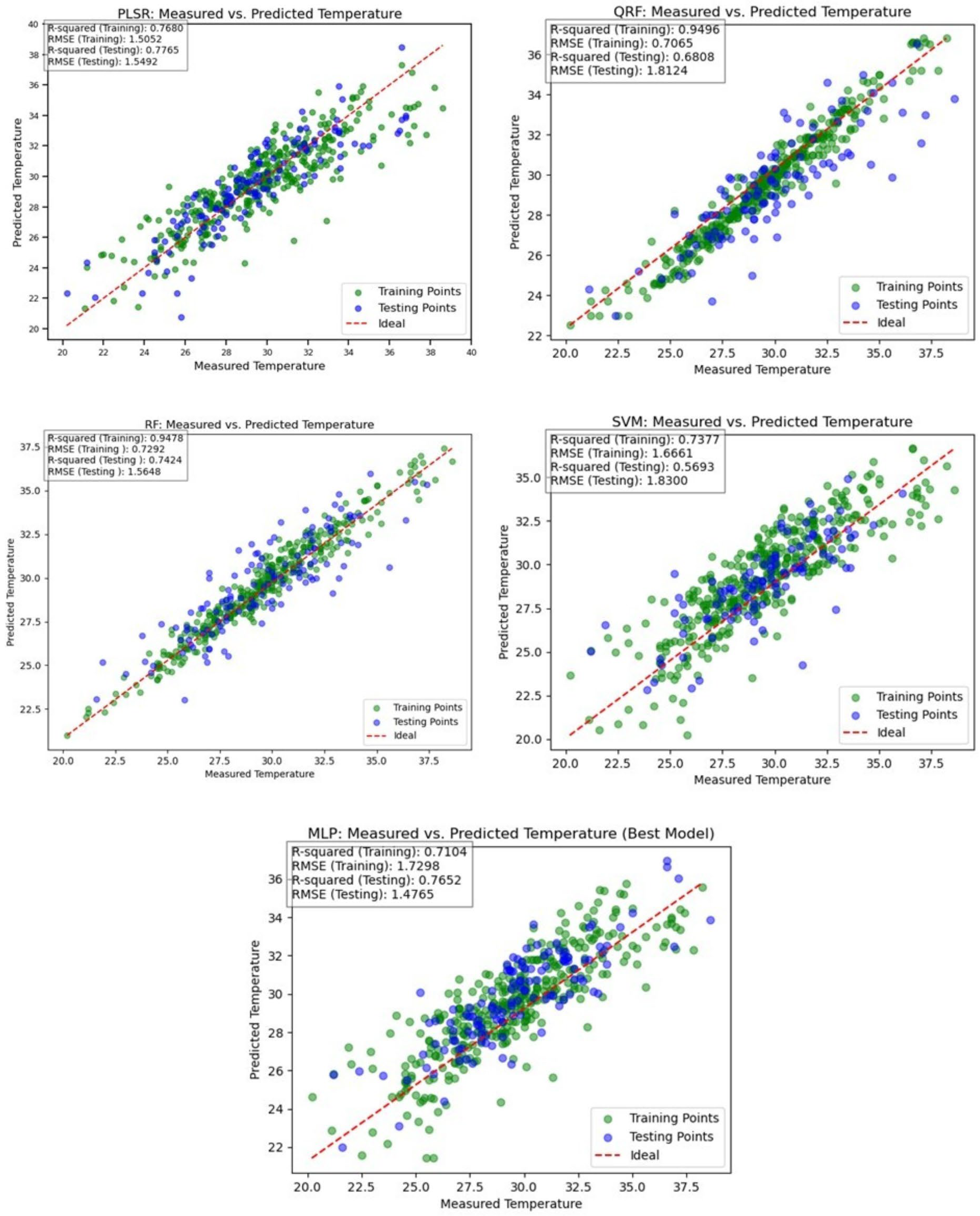
Figure 3 illustrates the results of the prediction of Tair using the mentioned models. Hence, both RF and QRF models demonstrated robust performance across both training and testing datasets. They exhibited high training R2 values, indicating an effective capture of relationships within the training data. Their low RMSEtrain values further confirm their strong fit. Of all models, RF achieved the highest testing R2 of 0.74 and the lowest RMSEtest of 0.56, highlighting its superior ability to generalize to unseen data. While QRF’s testing R2 was slightly lower than RF’s, its RMSEtest of 1.81 suggests some generalization challenges, though its performance remained reasonable. This difference is consistent with the methodological distinction between RF, which estimates the conditional mean, and QRF, which estimates the full conditional distribution through quantiles. Although the models achieved high training accuracy, its lower testing performance likely reflects data variability and the limited number of ground stations. Table 3 shows that RF achieved the lowest test RMSE, while PLSR had the highest test R2. This apparent discrepancy reflects the different aspects captured by these metrics: RMSE quantifies the absolute magnitude of prediction errors, which is critical for spatial mapping applications where minimizing local deviations is important, whereas R2 reflects the proportion of variance explained across all samples [33,54].
Conversely, SVN and MLP models showed weaker performance. Their training R2 values were notably lower, coupled with higher RMSEtrain values. The SVM model displayed a lower testing R2 and a higher RMSEtest, indicating poor generalization and larger prediction errors on the test data, suggesting it may not be suitable for this prediction task. Although the MLP exhibited a competitive testing R2 of 0.76, its RMSEtest of 1.47 indicates moderate prediction errors, and it did not consistently outperform the RF and QRF models.
Overall, the RF model emerged as the best performer, demonstrating an effective balance between bias and variance across both training and testing phases. This superior performance can be attributed to its ability to capture complex nonlinear relationships between environmental predictors and Tair, which are particularly pronounced in heterogeneous urban environments such as Yerevan. QRF also performed well, albeit with some limitations in generalization; however, its ability to estimate the full conditional distribution of Tair provides additional value through uncertainty quantification, which is important in spatial modeling. In contrast, SVM proved significantly limited, likely due to its sensitivity to parameter selection and reduced flexibility in handling highly complex spatial interactions. While MLP showed decent testing performance, it lacked the overall robustness and stability of the tree-based models, possibly due to the relatively small dataset and risk of overfitting. These results highlight the advantage of ensemble tree-based methods for modeling urban temperature in complex terrain conditions characterized by strong spatial variability and limited observational data.
Considering the results of a previous study by Tepanosyan et al. (2023), where the Partial Least Squares Regression (PLSR) model was applied for urban Tair estimation and temporal prediction with satisfactory results, its suitability for spatial mapping was re-evaluated [48]. Based on the comparative performance observed un this study, PLSR, QRF and FR were selected for the mapping of Tair distribution in Yerevan. The other methods—SVM and MLP were deemed not worth further consideration for subsequent research stages and were therefore dropped.

3.2. Mapping of Urban Tair

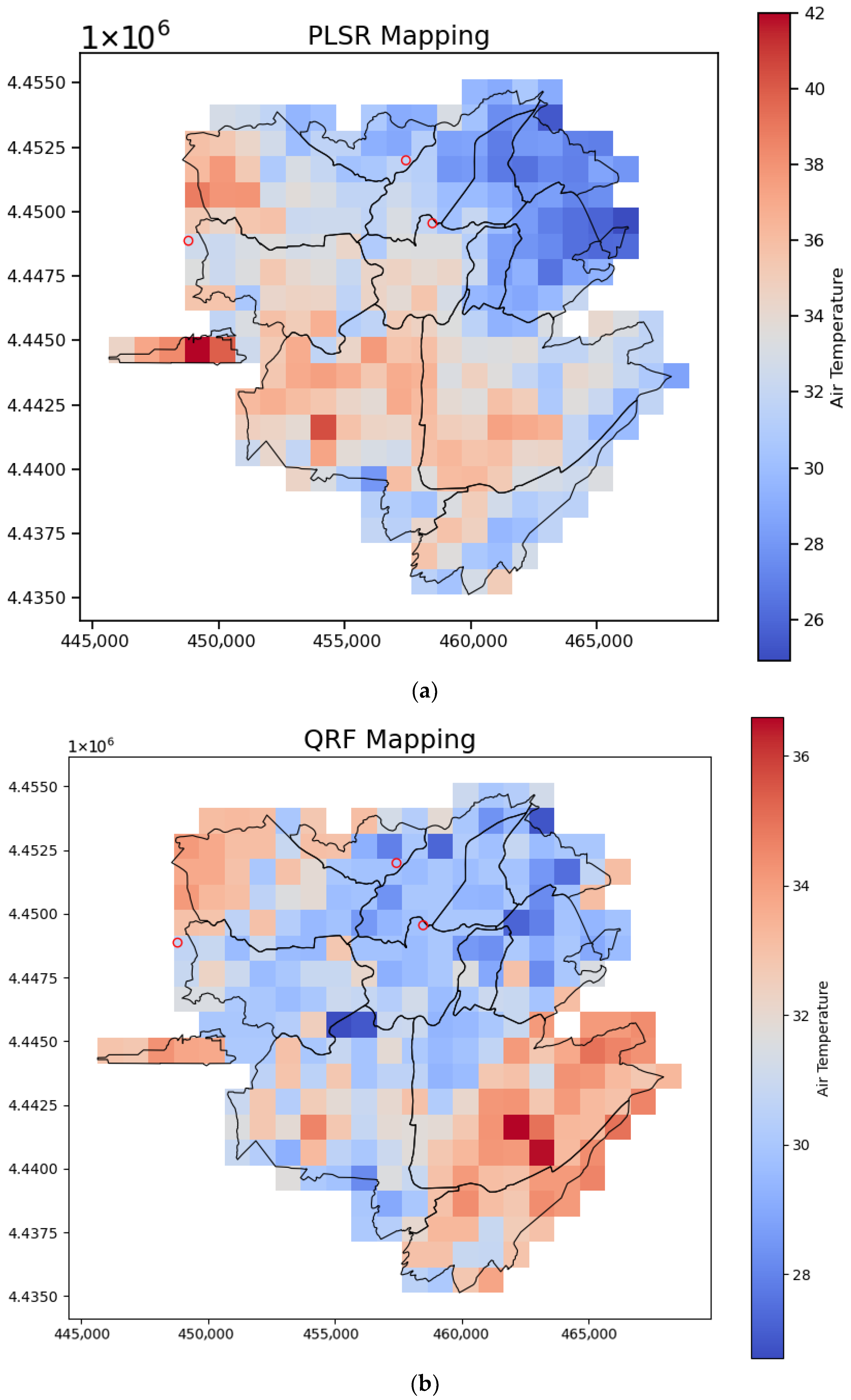
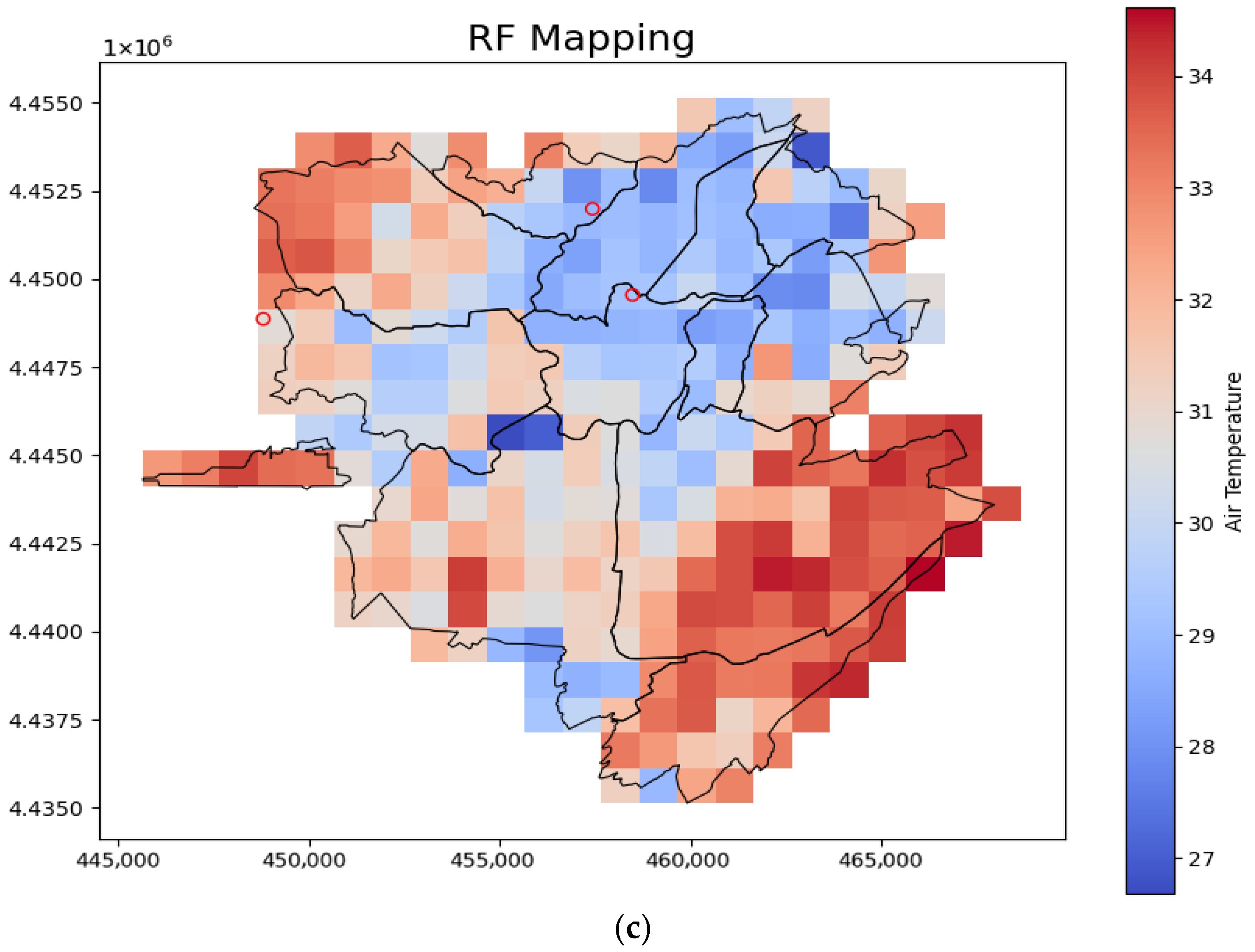
Models trained on historical data were applied throughout the city to build maps of estimated temperatures, providing comprehensive spatial insights rather than just single local estimates. The maps presented in this subsection illustrate the spatial distribution of absolute temperature values across the study area on 27 July 2020 (Figure 4).
The RF model presents a temperature range between 27 °C and 34 °C. The highest temperatures (32 °C to 34 °C) are predominantly found in the southeastern, western and northwestern parts pf the map, particularly the southwest corners, indicating the warmest conditions. Cooler zones reflecting temperatures between 27 °C and 30 °C are mostly distributed in central, northern and eastern areas. Moderate temperatures (30 °C to 32 °C) serve as transition zones between cooler and warmer areas, occupying most of central and southern parts of the map.
The PLSR map reveals significant Tair variations, with values broadly ranging from approximately from 26 °C to 42 °C. Relatively lower temperatures, mostly between 26 °C and 32 °C are observed in the northern and eastern parts of city. In contrast, the central, western, and southern regions are notably warmer, with temperatures typically between 34 °C and 40 °C, and a few isolated spots in the extreme west even exceeding 40 °C. Average temperature zones (30 °C to 34 °C) are represented around the central areas.
In the case of QRF model, Tair spans a narrower range, from 28 °C to 36 °C. Cooler areas, specifically those between 28 °C and 30 °C are primarily towards the northern and north-central parts, experiencing significantly lower temperatures. Temperatures between 30 °C and 32 °C are widely distributed across the central part, indicating a moderate temperature range. Transition zones (32 °C to 34 °C) between cooler and warmer regions are spread across several parts, signifying moderately warm areas. The warmest areas with temperature between 34 °C and 36 °C are mainly found in the southern and southeastern parts. These higher temperatures are likely influenced by local climatic and geographic factors such as higher solar radiation and lower elevation, with the southeastern part showing the highest temperatures, around 36 °C. Notably, QRF’s mapping accuracy is further supported by the absence of an anomalously warm region in the northernmost part of the map, a feature observed in other models, as this vegetated area should inherently be cooler than its surroundings.
As seen on Figure 4 across all three models, a consistent pattern emerges: a cooler north and northeast, corresponding to densely urbanized parts [46] on higher altitudes and a warmer south/southwest, likely indicating lower altitudes, less urbanized and with less vegetation, potentially reflecting urban heat islands with dry, exposed land surfaces.
The cooler northern temperatures, despite urbanization, are primarily due to the dominant effect of elevation. While the temperature transition between cooler and warmer regions is consistent across all maps, the intensity and overall temperature range vary slightly. PLSR exhibits a broader range of temperatures (26 °C to 42 °C), particularly with higher temperatures exceeding 40 °C notably in the western parts.
In contrast, QRF and RF show narrower temperature ranges (28 °C to 36 °C for QRF; 27 °C to 34 °C for RF) and a more uniform temperature distribution without extreme hot spots above 36 °C. PLSR, however, displays a more pronounced contrast between hot and cool regions, particularly emphasizing hotter conditions in the west more strongly than the more moderate temperatures predicted by QRF and RF in the same areas.
Complete variation in the estimated temperature maps is constrained by the limited availability of reference data. As an alternative, validation was addressed through two distinct and sensible checks. The focus was placed on 27 July 2020, as it was one of the hottest days on record, implying the strongest temperature contrast across the urban area. First, the accuracy of pointwise predictions was assessed. Actual temperatures recorded at the tree weather stations were compared with the Tair values obtained from the corresponding grid cells (tiles) at the station locations. The results (presented in a table within the study) indicate that Tair values obtained from all three models do not differ significantly from the in situ measurements. Notably, the PLSR model demonstrated the highest reliability, showing a difference in only 0.3–1.9 °C. However, the result of the RF model seems to be more robust in terms of a range of temperatures around 7 °C and a reasonable spatial distribution. In addition, a cold spot is observed to the south-west of the city center, where an extensive water reservoir (Yerevanian lake) is located, justifying a lower temperature with respect to surrounding area. Second, the spatial patterns of the predicted temperatures were examined for corrections based on known geographical and urban features. The highest Tairs are observed in the southwestern and western parts of the city, likely influenced by the presence of the Erebuni and Zvartnots airfields, respectively, and potentially industrial areas. Conversely, the lowest temperatures, seen near the city center and northeast, can be attributed to the cooling effects of the Hrazdan river valley, Yerevanian lake, and Dalma Gardens, where two of these latter being characterized by dense vegetation. Furthermore, the maps clearly show relatively lower Tairs in the northwest, which is consistent with the area’s higher elevation, including a noticeable cold spot within the Hrazdan river gorge at the northeast end.
A comparative analysis of several ML models revealed that RF and QRF consistently demonstrated good predictive capabilities, both in training and testing phases. Notably, QRF appears suitable as a spatial predictor of urban Tair, not only exhibiting robust statistical performance but also accurately reflecting known microclimatic features, such as cooler vegetated areas, which were sometimes anomalous in the outputs of other models. While PLSR also showed reliability in pointwise predictions, QRF and RF provided more uniform and consistent spatial distributions, avoiding the extreme seen in some PLSR-based maps. The validation against in situ station data and the consistency of predicted spatial patterns with known geographical and urban features further support the reliability of the models, particularly QRF, for mapping Tair. The accuracy achieved for Tair mapping in this study is comparable to, and in some cases, superior to other published works in the field.

4. Limitations

The main limitation of this study is the limited number of ground stations and their uneven distribution, which is particularly significant for a city with such complex terrain as Yerevan. A primary constraint was the limited availability of ground reference data for spatial validation—while the three existing weather stations provided pointwise validation, a denser network, potentially enlarged by additional sources such as mobile weather stations, would enable more comprehensive and robust quantitative validation across the highly heterogeneous urban landscape. Consequently, the validation performed was qualitative to some extent, relying also on local knowledge and expert interpretation of temperature patterns in addition to independent measurements. This limits the definitive quantitative assessment of the accuracy of spatial maps beyond the immediate vicinity of the few fixed stations.

5. Conclusions

This study investigated the application of different ML models for predicting the spatial distribution of urban Tair in Yerevan, which is characterized by its complex terrain and limited ground-based meteorological data. The research demonstrated the effectiveness of remote sensing data and advanced ML algorithms in overcoming the limitations of traditional sparse weather station network for detailed Tair mapping.
Among the evaluated models, RF and QRF demonstrated the most reliable spatial predictions of Tair, with RF achieving the best quantitative performance and QRF most accurately reflecting known microclimatic features of Yerevan’s urban landscape.
Despite the promising results, certain limitations of this study warrant acknowledgment. A primary constraint was the limited availability of ground reference data. While existing weather stations provided some validation points, a denser network, potentially enlarged by other sources of temperature data potentially including mobile weather stations, would enable more comprehensive and robust quantitative validation across the highly heterogeneous urban landscape. Consequently, the validation performed was qualitative to some extent, relying also on local knowledge and expert interpretation of temperature patterns in addition to independent measurements. This limits the definitive quantitative assessment of the accuracy of spatial maps beyond the immediate vicinity of the few fixed stations.
Terrain complexity plays an important role in shaping the spatial performance of the model, as heterogeneous topography—such as steep slopes and strong elevation gradients—introduces increased variability in prediction accuracy. This variability is mainly driven by stronger spatial discontinuities and localized microclimatic effects, which are more difficult to represent using the available input data. As a result, model outputs are not fully uniform across the study domain, with noticeable performance differences between relatively flat and highly complex terrain areas. Nevertheless, the model maintains stable overall predictive skill, indicating good general robustness.
Further research could explore several avenues:
  • Integrating more diverse and higher-resolution remote sensing data, such as hyperspectral imagery or LiDAR data, could further refine Tair predictions, especially in highly heterogeneous urban landscapes.
  • Integrating additional environmental variables including wind rose and precipitation.
  • Investigating the diurnal and seasonal variations in the urban heat island effect using these advanced mapping techniques would provide a more dynamic understanding of urban climate of Yerevan.
  • Also, the developed methodologies could be applied to other complex urban environments with similar data scarcity challenges, contributing to boarder efforts in climate change adaptation and urban planning.
This research, therefore, provides some basis for developing more accurate and spatially comprehensive urban thermal monitoring system vital for effective climate action and sustainable urban development in Yerevan.

Author Contributions

Conceptualization, V.M., S.A. and F.D.; Methodology, V.M. and F.D.; Investigation, V.M., S.A., R.A., G.T. and F.D.; Validation, R.A., A.K. and A.B.; Formal Analysis, R.A., A.K., A.H., G.T. and A.B.; Resources, S.A. and F.D.; Data Curation, V.M., R.A., A.H., G.T. and A.B.; Writing—Original Draft Preparation, V.M., S.A. and F.D.; Writing—Review & Editing, V.M., S.A. and F.D.; Visualization, R.A., A.H. and A.K.; Supervision, S.A. and F.D.; Funding Acquisition, S.A. and F.D. All authors have read and agreed to the published version of the manuscript.

Funding

This study was supported by the Higher Education and Science Committee of the Ministry of Education, Science, Sport and Culture of RA in the framework of the research project No.23LCG_1E016. This work was partly funded by the European Union—“NextGenerationEU, Mission 4 Component 1.5—ECS00000036—CUP F17G22000190007” and Italian Ministry of University and Research, DD 307 project MI567 “QUANTAS”.

Institutional Review Board Statement

Not applicable.

Informed Consent Statement

Not applicable.

Data Availability Statement

The data that support the findings of this study are available on request from the corresponding author.

Acknowledgments

The authors would like to acknowledge the Department of GIS and Remote Sensing of the Center for Ecological-Noosphere Studies of the National Academy of Sciences (Armenia) as well as the Department of Electrical, Computer and Biomedical Engineering at the University of Pavia, Italy, for providing the facilities necessary to conduct this research. The Authors also acknowledge the use of the AI Google Gemini 2025 for language editing and text refinement. All scientific content, interpretations, and conclusions are the sole responsibility of the authors.

Conflicts of Interest

The authors declare no conflicts of interest.

Abbreviations

The following abbreviations are used in this manuscript:
LSTLand surface temperature
MLMachine learning
PLSRPartial Least-Squares Regression
RFRandom forest
QRFQuantile regression forest
SVMSupport vector machine
MLPMultiLayer Perception
RMSERoot Mean Square Error
UHIUrban Heat Island
TIRThermal InfraRed
TVXTemperature Vegetation Index
RSRemote Sensing
GISGeographic Information Systems
ANNArtificial Neural Network
GEEGoogle Earth Engine
NDVINormalized Difference Vegetation Index
NDWINormalized Difference Water Index
IBIIndex-based Build-up Index
SAVISoil-Adjusted Vegetation Index
DEMDigital Elevation Model
NIRNear Infrared
SWIRShortwave Infrared
DOYDay of Year
VIPVariable Importance in Projection

References

  1. Trenberth, K.E.; Zhang, Y.; Fasullo, J.T.; Taguchi, S. Climate Variability and Relationships between Top-of-Atmosphere Radiation and Temperatures on Earth. J. Geophys. Res. Atmos. 2015, 120, 3642–3659. [Google Scholar] [CrossRef]
  2. Ginzburg, A.S. Regional Air Temperature Maxima and the Possibility of Their Simple Energy-Balance Estimates. Izv. Atmos. Ocean. Phys. 2011, 47, 665–671. [Google Scholar] [CrossRef]
  3. Mahmoud, S.H.; Gan, T.Y. Impact of Anthropogenic Climate Change and Human Activities on Environment and Ecosystem Services in Arid Regions. Sci. Total Environ. 2018, 633, 1329–1344. [Google Scholar] [CrossRef]
  4. Kinney, P.L. Climate Change, Air Quality, and Human Health. Am. J. Prev. Med. 2008, 35, 459–467. [Google Scholar] [CrossRef]
  5. Mirzaei, P.A. Recent Challenges in Modeling of Urban Heat Island. Sustain. Cities Soc. 2015, 19, 200–206. [Google Scholar] [CrossRef]
  6. Heisler, G.M.; Brazel, A.J. The Urban Physical Environment: Temperature and Urban Heat Islands. In Urban Ecosystem Ecology; John Wiley & Sons, Ltd.: Hoboken, NJ, USA, 2010; pp. 29–56. [Google Scholar]
  7. Ding, L.; Zhou, J.; Zhang, X.; Liu, S.; Cao, R. Downscaling of Surface Air Temperature over the Tibetan Plateau Based on DEM. Int. J. Appl. Earth Obs. Geoinf. 2018, 73, 136–147. [Google Scholar] [CrossRef]
  8. dos Santos, R.S. Estimating Spatio-Temporal Air Temperature in London (UK) Using Machine Learning and Earth Observation Satellite Data. Int. J. Appl. Earth Obs. Geoinf. 2020, 88, 102066. [Google Scholar] [CrossRef]
  9. Nichol, J.E.; To, P.H. Temporal Characteristics of Thermal Satellite Images for Urban Heat Stress and Heat Island Mapping. ISPRS J. Photogramm. Remote Sens. 2012, 74, 153–162. [Google Scholar] [CrossRef]
  10. Rahmatollahi, N.; Wang, Z.-H.; Wang, Y.; Yang, X. Machine Learning and Causal Attribution of Urban Heat in the Phoenix Metropolitan. Sustain. Cities Soc. 2026, 137, 107145. [Google Scholar] [CrossRef]
  11. Abbas, A.; He, Q.; Jin, L.; Li, J.; Salam, A.; Lu, B.; Yasheng, Y. Spatio-Temporal Changes of Land Surface Temperature and the Influencing Factors in the Tarim Basin, Northwest China. Remote Sens. 2021, 13, 3792. [Google Scholar] [CrossRef]
  12. Voogt, J.A.; Oke, T.R. Thermal Remote Sensing of Urban Climates. Remote Sens. Environ. 2003, 86, 370–384. [Google Scholar] [CrossRef]
  13. Vogt, J.V.; Viau, A.A.; Paquet, F. Mapping Regional Air Temperature Fields Using Satellite-Derived Surface Skin Temperatures. Int. J. Climatol. 1997, 17, 1559–1579. [Google Scholar] [CrossRef]
  14. Zakšek, K.; Schroedter-Homscheidt, M. Parameterization of Air Temperature in High Temporal and Spatial Resolution from a Combination of the SEVIRI and MODIS Instruments. ISPRS J. Photogramm. Remote Sens. 2009, 64, 414–421. [Google Scholar] [CrossRef]
  15. Benali, A.; Carvalho, A.C.; Nunes, J.P.; Carvalhais, N.; Santos, A. Estimating Air Surface Temperature in Portugal Using MODIS LST Data. Remote Sens. Environ. 2012, 124, 108–121. [Google Scholar] [CrossRef]
  16. Chen, X.; Zhang, Y. Impacts of Urban Surface Characteristics on Spatiotemporal Pattern of Land Surface Temperature in Kunming of China. Sustain. Cities Soc. 2017, 32, 87–99. [Google Scholar] [CrossRef]
  17. Yang, G.; Sun, W.; Shen, H.; Meng, X.; Li, J. An Integrated Method for Reconstructing Daily MODIS Land Surface Temperature Data. IEEE J. Sel. Top. Appl. Earth Obs. Remote Sens. 2019, 12, 1026–1040. [Google Scholar] [CrossRef]
  18. Chen, Y.; Amani-Beni, M.; Chen, C.; Liang, Y.; Li, J.; Yang, L. Projection of Urban Land Surface Temperature: An Inter- and Intra-Annual Modeling Approach. Urban Clim. 2023, 51, 101637. [Google Scholar] [CrossRef]
  19. Ho, H.C.; Knudby, A.; Sirovyak, P.; Xu, Y.; Hodul, M.; Henderson, S.B. Mapping Maximum Urban Air Temperature on Hot Summer Days. Remote Sens. Environ. 2014, 154, 38–45. [Google Scholar] [CrossRef]
  20. Vancutsem, C.; Ceccato, P.; Dinku, T.; Connor, S.J. Evaluation of MODIS Land Surface Temperature Data to Estimate Air Temperature in Different Ecosystems over Africa. Remote Sens. Environ. 2010, 114, 449–465. [Google Scholar] [CrossRef]
  21. Weng, Q. Thermal Infrared Remote Sensing for Urban Climate and Environmental Studies: Methods, Applications, and Trends. ISPRS J. Photogramm. Remote Sens. 2009, 64, 335–344. [Google Scholar] [CrossRef]
  22. Agam, N.; Kustas, W.P.; Anderson, M.C.; Li, F.; Neale, C.M.U. A Vegetation Index Based Technique for Spatial Sharpening of Thermal Imagery. Remote Sens. Environ. 2007, 107, 545–558. [Google Scholar] [CrossRef]
  23. Nieto, H.; Sandholt, I.; Aguado, I.; Chuvieco, E.; Stisen, S. Air Temperature Estimation with MSG-SEVIRI Data: Calibration and Validation of the TVX Algorithm for the Iberian Peninsula. Remote Sens. Environ. 2011, 115, 107–116. [Google Scholar] [CrossRef]
  24. Ozelkan, E.; Bagis, S.; Ozelkan, E.C.; Ustundag, B.B.; Yucel, M.; Ormeci, C. Spatial Interpolation of Climatic Variables Using Land Surface Temperature and Modified Inverse Distance Weighting. Int. J. Remote Sens. 2015, 36, 1000–1025. [Google Scholar] [CrossRef]
  25. Parmentier, B.; McGill, B.J.; Wilson, A.M.; Regetz, J.; Jetz, W.; Guralnick, R.; Tuanmu, M.-N.; Schildhauer, M. Using Multi-Timescale Methods and Satellite-Derived Land Surface Temperature for the Interpolation of Daily Maximum Air Temperature in Oregon. Int. J. Climatol. 2015, 35, 3862–3878. [Google Scholar] [CrossRef]
  26. Li, X.Y.; Li, Z.; Zhang, Q.Q.; Zhou, P.X.; Huang, W. Prediction of Long-Term Near-Surface Temperature Based on NA-CORDEX Output. J. Environ. Inform. Lett. 2019, 2, 10–18. [Google Scholar] [CrossRef]
  27. Florio, E.N.; Lele, S.R.; Chi Chang, Y.; Sterner, R.; Glass, G.E. Integrating AVHRR Satellite Data and NOAA Ground Observations to Predict Surface Air Temperature: A Statistical Approach. Int. J. Remote Sens. 2004, 25, 2979–2994. [Google Scholar] [CrossRef]
  28. Bechtel, B.; Zakšek, K.; Oßenbrügge, J.; Kaveckis, G.; Böhner, J. Towards a Satellite Based Monitoring of Urban Air Temperatures. Sustain. Cities Soc. 2017, 34, 22–31. [Google Scholar] [CrossRef]
  29. Yang, Y.Z.; Cai, W.H.; Yang, J. Evaluation of MODIS Land Surface Temperature Data to Estimate Near-Surface Air Temperature in Northeast China. Remote Sens. 2017, 9, 410. [Google Scholar] [CrossRef]
  30. Good, E.J.; Ghent, D.J.; Bulgin, C.E.; Remedios, J.J. A Spatiotemporal Analysis of the Relationship between Near-Surface Air Temperature and Satellite Land Surface Temperatures Using 17 Years of Data from the ATSR Series. J. Geophys. Res. Atmos. 2017, 122, 9185–9210. [Google Scholar] [CrossRef]
  31. Xu, Y.; Knudby, A.; Ho, H.C. Estimating Daily Maximum Air Temperature from MODIS in British Columbia, Canada. Int. J. Remote Sens. 2014, 35, 8108–8121. [Google Scholar] [CrossRef]
  32. Liu, L.; Zhang, Y. Urban Heat Island Analysis Using the Landsat TM Data and ASTER Data: A Case Study in Hong Kong. Remote Sens. 2011, 3, 1535–1552. [Google Scholar] [CrossRef]
  33. Yoo, C.; Im, J.; Park, S.; Quackenbush, L.J. Estimation of Daily Maximum and Minimum Air Temperatures in Urban Landscapes Using MODIS Time Series Satellite Data. ISPRS J. Photogramm. Remote Sens. 2018, 137, 149–162. [Google Scholar] [CrossRef]
  34. Rasul, A.; Balzter, H.; Smith, C. Applying a Normalized Ratio Scale Technique to Assess Influences of Urban Expansion on Land Surface Temperature of the Semi-Arid City of Erbil. Int. J. Remote Sens. 2017, 38, 3960–3980. [Google Scholar] [CrossRef]
  35. Nikoloudakis, N.; Stagakis, S.; Mitraka, Z.; Kamarianakis, Y.; Chrysoulakis, N. Spatial Interpolation of Urban Air Temperatures Using Satellite-Derived Predictors. Theor. Appl. Clim. 2020, 141, 657–672. [Google Scholar] [CrossRef]
  36. Cristóbal, J.; Jiménez-Muñoz, J.C.; Prakash, A.; Mattar, C.; Skoković, D.; Sobrino, J.A. An Improved Single-Channel Method to Retrieve Land Surface Temperature from the Landsat-8 Thermal Band. Remote Sens. 2018, 10, 431. [Google Scholar] [CrossRef]
  37. Mutiibwa, D.; Strachan, S.; Albright, T. Land Surface Temperature and Surface Air Temperature in Complex Terrain. IEEE J. Sel. Top. Appl. Earth Obs. Remote Sens. 2015, 8, 4762–4774. [Google Scholar] [CrossRef]
  38. Orellana-Samaniego, M.L.; Ballari, D.; Guzman, P.; Ospina, J.E. Estimating Monthly Air Temperature Using Remote Sensing on a Region with Highly Variable Topography and Scarce Monitoring in the Southern Ecuadorian Andes. Theor. Appl. Clim. 2021, 144, 949–966. [Google Scholar] [CrossRef]
  39. Cifuentes, J.; Marulanda, G.; Bello, A.; Reneses, J. Air Temperature Forecasting Using Machine Learning Techniques: A Review. Energies 2020, 13, 4215. [Google Scholar] [CrossRef]
  40. Agathangelidis, I.; Cartalis, C.; Santamouris, M. Estimation of Air Temperatures for the Urban Agglomeration of Athens with the Use of Satellite Data. Geoinform. Geostat. Overv. 2016, 4, 2. [Google Scholar] [CrossRef]
  41. Meliho, M.; Khattabi, A.; Zejli, D.; Orlando, C.A.; Dansou, C.E. Artificial Intelligence and Remote Sensing for Spatial Prediction of Daily Air Temperature: Case Study of Souss Watershed of Morocco. Geo-Spat. Inf. Sci. 2022, 25, 244–258. [Google Scholar] [CrossRef]
  42. Zhang, G.; Bateni, S.M.; Jun, C.; Khoshkam, H.; Band, S.S.; Mosavi, A. Feasibility of Random Forest and Multivariate Adaptive Regression Splines for Predicting Long-Term Mean Monthly Dew Point Temperature. Front. Environ. Sci. 2022, 10, 826165. [Google Scholar] [CrossRef]
  43. Tepanosyan, G.; Muradyan, V.; Hovsepyan, A.; Pinigin, G.; Medvedev, A.; Asmaryan, S. Studying Spatial-Temporal Changes and Relationship of Land Cover and Surface Urban Heat Island Derived through Remote Sensing in Yerevan, Armenia. Build. Environ. 2021, 187, 107390. [Google Scholar] [CrossRef]
  44. Riley, S.J.; De Gloria, S.D.; Elliot, R. A Terrain Ruggedness Index That Quantifies Topographic Heterogeneity. Intermt. J. Sci. 1999, 5, 23–27. [Google Scholar]
  45. Zhang, H.; Zhang, F.; Ye, M.; Che, T.; Zhang, G. Estimating Daily Air Temperatures over the Tibetan Plateau by Dynamically Integrating MODIS LST Data. J. Geophys. Res. Atmos. 2016, 121, 11,425–11,441. [Google Scholar] [CrossRef]
  46. Noi, P.T.; Kappas, M.; Degener, J. Estimating Daily Maximum and Minimum Land Air Surface Temperature Using MODIS Land Surface Temperature Data and Ground Truth Data in Northern Vietnam. Remote Sens. 2016, 8, 1002. [Google Scholar] [CrossRef]
  47. Otgonbayar, M.; Atzberger, C.; Mattiuzzi, M.; Erdenedalai, A. Estimation of Climatologies of Average Monthly Air Temperature over Mongolia Using MODIS Land Surface Temperature (LST) Time Series and Machine Learning Techniques. Remote Sens. 2019, 11, 2588. [Google Scholar] [CrossRef]
  48. Tepanosyan, G.; Asmaryan, S.; Muradyan, V.; Avetisyan, R.; Hovsepyan, A.; Khlghatyan, A.; Ayvazyan, G.; Dell’Acqua, F. Machine Learning-Based Modeling of Air Temperature in the Complex Environment of Yerevan City, Armenia. Remote Sens. 2023, 15, 2795. [Google Scholar] [CrossRef]
  49. Belgiu, M.; Drăguţ, L. Random Forest in Remote Sensing: A Review of Applications and Future Directions. ISPRS J. Photogramm. Remote Sens. 2016, 114, 24–31. [Google Scholar] [CrossRef]
  50. Breiman, L. Random Forests. Mach. Learn. 2001, 45, 5–32. [Google Scholar] [CrossRef]
  51. Meinshausen, N. Quantile Regression Forests. J. Mach. Learn. Res. 2006, 7, 983–999. [Google Scholar]
  52. Awad, M.; Khanna, R. Support Vector Machines for Classification. In Efficient Learning Machines: Theories, Concepts, and Applications for Engineers and System Designers; Awad, M., Khanna, R., Eds.; Apress: Berkeley, CA, USA, 2015; pp. 39–66. [Google Scholar]
  53. Atkinson, P.M.; Tatnall, A.R.L. Introduction Neural Networks in Remote Sensing. Int. J. Remote Sens. 1997, 18, 699–709. [Google Scholar] [CrossRef]
  54. Hastie, T.; Tibshirani, R.; Friedman, J. The Elements of Statistical Learning; Springer Series in Statistics; Springer: New York, NY, USA, 2009. [Google Scholar]
Figure 1. Geographical location of Yerevan city and the distribution of the weather stations: (1) Yerevan_agro; (2) Yerevan_aerologia; (3) Arabkir.
Urbansci 10 00257 g001
Figure 2. Methodological flowchart of the study.
Urbansci 10 00257 g002
Figure 3. Comparison of the performance (measured vs. predicted) Models (PLSR, QRF, RF, SVM, MLP) for Tair prediction.
Urbansci 10 00257 g003
Figure 4. Spatial mapping of predicted Tair using regression models for 27 July 2020: (a) PLSR; (b) QRF; (c) RF. The red circles are indicating locations of weather stations.
Urbansci 10 00257 g004aUrbansci 10 00257 g004b
Table 1. Description and relevance of variables used for urban Tair modeling.
CategoryVariableDescription/SourceRelevance to Tair Assessment
Spectral Bands
(Landsat 4–8)
Blue, Green, Red, NIR, SWIR1, SWIR2Surface reflectance bands from Landsat missions (TM, ETM+, OLI/TIRS)Represent surface material and albedo differences; influence surface energy absorption and heat emission patterns.
Spectral IndicesNDVI (Normalized Difference
Vegetation Index)
(NIR − Red)/(NIR + Red)Indicates vegetation density; higher NDVI corresponds to cooler areas due to evapotranspiration.
NDWI (Normalized Difference Water Index)(NIR − SWIR)/(NIR + SWIR)Detects water and moisture content; areas with higher NDWI are cooler.
IBI-SAVI (Index-Based Built-Up Index and Soil-Adjusted Vegetation Index)IBI-SAVI = (((NDBI + 1) − ((SAVI + 1) + (MNDWI + 1))/2))/(((NDBI + 1) + ((SAVI + 1) + (MNDWI + 1))/2))Captures urban surface composition; higher IBI-SAVI values are associated with greater impervious surface coverage and elevated Tair.
Thermal VariableLST (Land Surface Temperature)Derived from Landsat TIR bands (OLI/TIRS)Strongest satellite-based predictor of near-surface Tair; directly related to surface–atmosphere heat exchange.
Topographic
Factors (DEM-derived)
ElevationFrom digital elevation model (DEM)Affects Tair through lapse rate; higher elevations are typically cooler.
SlopeDEM-derived gradientInfluences insolation and air flow; steeper slopes may experience reduced solar heating.
AspectDEM-derived orientationControls solar radiation exposure; south-facing slopes in Yerevan receive more sunlight and are warmer.
Terrain Ruggedness IndexFrom DEM [44]Quantifies surface heterogeneity; affects local wind and heat distribution.
Solar RadiationComputed from DEM using solar geometryMajor driver of surface and Tair; varies with slope, aspect, and season.
Statistical MetricsMean of each
variable listed above
Mean value of variable within 1 km grid cellCaptures average environmental condition influencing Tair.
Standard deviation of each variable listed aboveSD within 1 km grid cellRepresents local variability and surface heterogeneity, which influence microclimate and heat retention.
Temporal FactorDOY (Day of Year)Acquisition day of Landsat imageReflects seasonal variability in solar radiation and atmospheric conditions.
Table 2. Final hyperparameter settings used for each machine learning model.
ML ModelsFinal Hyperparameter Settings Parameters
PLSR
  • n_components: 10
  • scale: True (default)
  • max_iter: 500 (default)
  • tol: 1 × 10⁻⁶ (default)
RF
  • n_estimators: 100
  • random_state: 50
  • max_depth: None (default, trees grow until all leaves are pure)
  • min_samples_split: 2 (default)
  • min_samples_leaf: 1 (default)
  • max_features: 1.0 (default, all features considered)
QRF
  • n_estimators: 500 (optimized via GridSearchCV)
  • random_state: 42
  • min_samples_split: 10 (optimized via GridSearchCV)
  • max_features: ‘auto’ (optimized via GridSearchCV, equivalent to 1.0)
  • Quantiles predicted: 5th and 95th percentiles for uncertainty intervals
SVM
  • kernel: ‘linear’
  • C (regularization): 2.0
  • epsilon: 0.1 (default)
  • gamma: ‘scale’ (default)
MLP
  • hidden_layer_sizes: (100, 50)—two hidden layers with 100 and 50 neurons
  • activation: ‘relu’
  • solver: ‘lbfgs’ (Limited-memory BFGS optimizer)
  • alpha (L2 regularization): 0.0001
  • learning_rate: ‘constant’
  • max_iter: 1000
  • random_state: 1
Table 3. Performance metrics of models.
ML ModelR2trainR2testRMSEtrain(°C)RMSEtest(°C)
QRF0.950.680.711.81
RF0.940.740.730.56
SVM0.740.561.661.83
MLP0.710.761.731.47
PLSR0.770.781.501.54
Disclaimer/Publisher’s Note: The statements, opinions and data contained in all publications are solely those of the individual author(s) and contributor(s) and not of MDPI and/or the editor(s). MDPI and/or the editor(s) disclaim responsibility for any injury to people or property resulting from any ideas, methods, instructions or products referred to in the content.