Towards Water and Energy Security in Rural Agriculture: Technical Analysis of an Autonomous Photovoltaic Pumping System

Abstract

This study evaluates the technical feasibility of an autonomous photovoltaic pumping system for agricultural use in isolated communities, using a representative region of the Mixteca Poblana, Mexico, as a case study. A reference sizing methodology reported in the literature was adopted for the sizing of isolated systems, and subsequently enhanced through a structured methodological extension, applied in the final stage of the design, focused on the technical validation and commercial selection of system components. The base framework incorporates site characterization and crop selection criteria. Subsequent stages define the hydraulic and electrical design requirements for the extension of the methodology, such as the calculation of water demand, the determination of pump power, and the estimation of energy requirements. These parameters enable the integrated correlation between hydraulic demand and electrical system constraints in the selection of the main system components, including the pump, photovoltaic array, battery storage system, water storage tank, and inverter. The technical robustness of the combined approach was validated through a simulation performed using specialized solar pumping software, confirming the operational feasibility and replication potential in rural communities with similar conditions.

1. Introduction

At present, most rural regions around the world depend on agriculture as their main economic activity, and a lack of electricity, which hinders the optimal performance of tasks. For example, in 2019, of the world’s 7.67 billion inhabitants, approximately 760.89 million did not have access to this basic resource [1]. This profound energy inequality, which, according to recent studies, affects 17% of the world’s population, is concentrated in rural areas (85%). In countries such as Nigeria, for example, 22.6% of rural communities have access to electricity [2]. This segment of the community is limited in its economic and social development. In this context, access to water for irrigation or consumption becomes a structural problem, especially when the community’s water sources, whether springs or wells, require electric pumping, which also limits access to water.

The conventional solution is to extend the electricity grid; however, in isolated, sparsely populated communities, this approach entails high investment and operating costs, making it technically and economically infeasible. Studies have shown that in extremely isolated regions, operating costs exceed USD 30/kWh when the grid is extended, reinforcing the need for solutions that rely on alternative or renewable energy [3].

Solar photovoltaic (PV) powered water pumping systems offer a viable autonomous alternative, reducing dependence on fossil fuels and harnessing abundant solar energy in rural areas. These characteristics align them directly with Sustainable Development Goals (SDGs), including Goal 7 (Affordable and clean energy) by promoting access to clean energy, and Sustainable Development Goal 11 (Sustainable cities and communities) by strengthening the water and productive resilience of rural communities.

Within photovoltaic pumping systems, there are two main configurations: direct solar pumping and solar pumping assisted by lithium-ion (Li-ion) batteries. A study [4] evaluated these configurations, analyzing a pumping system comprising eight panels that supplied direct current (DC) to an inverter, which converted this energy to alternating current (AC) to power a 1.5 kW pump. The results showed that the system without batteries performed better overall, pumping 55.34 m³/day at a lower initial cost and with greater efficiency than the system with batteries, which pumped only 33.39 m³/day. However, the battery-based system could pump water on cloudy days or outside the operational irradiance window.

The coverage achieved by these systems highlights the need to continue improving their performance and reliability. In recent years (2021–2024), the literature has shifted toward optimizing both sizing processes and individual components to ensure the scalability of these solutions. Several studies have addressed this issue from different perspectives. For instance, in [5], an off-grid operation strategy was proposed that allows the system to continue operating during grid outages, achieving 100% efficiency in maximum power point tracking (MPPT) and switching times of less than 0.15 s. On the other hand, from a management perspective, the study in [6] integrated IoT technologies into photovoltaic pumping systems using sensors and microcontrollers, demonstrating that real-time optimization improves water distribution and promotes scalability in rural contexts.

Additionally, recent research has expanded the focus beyond electrical components. In [7], it was demonstrated that the incorporation of storage tanks enables total reliability in water supply (pIW = 0), in addition to reducing life-cycle costs through advanced optimization techniques. Likewise, in [8], the coupling between water demand and energy availability was optimized using dynamic programming, achieving reductions in operating costs of up to 30.5%.

Despite the advances described, a significant research gap remains. Most existing studies rely on the conventional methodology shown in Figure 1, which, while effective for general sizing, lacks a structured framework for the integrated selection of commercial components based on specific hydraulic variables. This absence of clear technical instructions complicates the implementation and dimensioning process for researchers and practitioners in rural contexts who may lack advanced specialized training. Furthermore, this lack of consistency leads to technical and economic problems that compromise the overall performance of the system and ultimately hinder its successful replication in different study cases.

Several studies show the consequences of choosing unsuitable components, thereby compromising the system’s objectives, such as in [11], where a system designed to cover 50 m³/day managed only 28.4% (14.21 m³/day) because the solar panel array was sized for 2.5 kW to power a 4 kW pump, but 8.82 kW was required for full operation. In turn, an expensive selection of certain components can delay or undermine the system’s economic recovery. In the case of [9], the selection of a battery costing CAD $72,800 increases costs by 30%, while a storage tank costing CAD $56,000 enables early recovery and greater benefits for agriculture. These results show that the problem does not lie in the individual size of each component but in a lack of coordinated technical selection among them.

The novelty of this research lies in the development of a structured methodological framework specifically designed for the integrated and technically appropriate selection of components for autonomous photovoltaic pumping systems. Unlike traditional approaches, this framework establishes a systematic relationship between hydraulic demand (crop water requirements and well characteristics) and electrical availability. By defining clear, replicable, and accessible criteria for the simultaneous sizing of the pump, the photovoltaic generator, battery storage, and the inverter, this study ensures technical synergy and economic viability. This methodology is designed to bridge the gap between complex engineering and practical application, facilitating high-performance designs in rural communities with limited water and energy resources. The resulting configuration was validated using high-fidelity numerical simulations in PVsyst v8.0.

The document is structured as follows: Section 2 presents the methodology and the proposed extension of the methodology. Subsequently, in Section 3, the technical validation of both approaches is carried out using the simulation results. Section 4 discusses the main contributions of the study and presents the general conclusions of the work.

2. Methodology

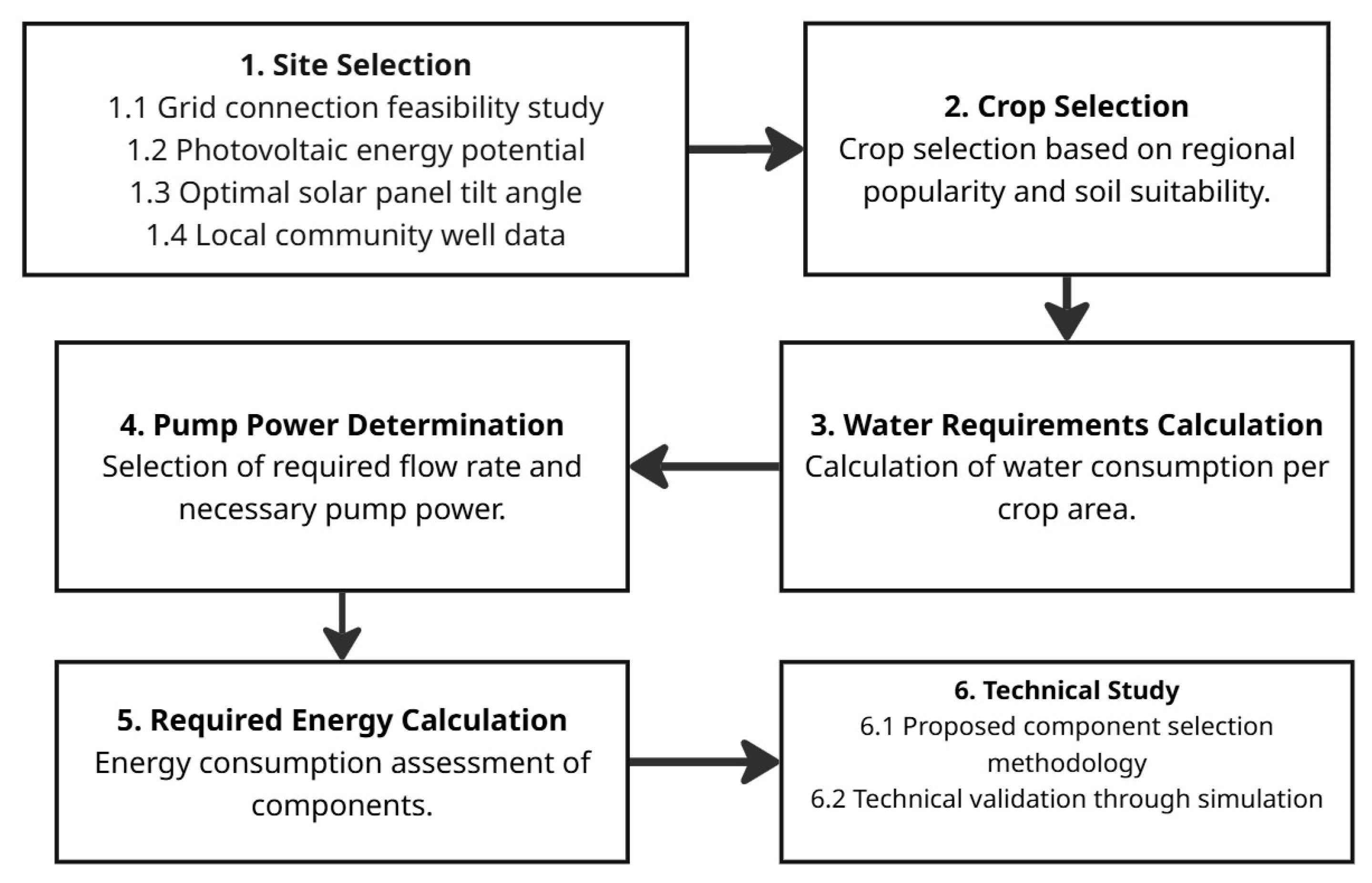
The fundamental methodology employed in this study is delineated in Figure 1, which details the general procedure utilized for comprehensive sizing, thereby furnishing essential criteria. Subsequently, Figure 2 proposes an extension of this basic methodology, specifically geared toward the technical selection of components for pumping systems. This approach enables precise sizing of commercial equipment, ensuring optimal use of each element and avoiding unnecessary oversizing.

Adhering to the structure delineated in Figure 1, the methodology is meticulously structured in a sequential manner. The first section presents the general methodology, where the system requirements are defined, including water demand, energy needs, and hydraulic constraints. Based on these results, Section 2.2 introduces the methodological extension, which uses the previously obtained parameters to guide the technical selection and integration of system components.

2.1. General Methodology

This section delineates the fundamental methodology, thereby establishing the criteria that function as a point of departure for methodological extension. The goal is for both approaches to work well together so that the basis and the extension can be validated by the results of the simulation.

2.1.1. Site Selection (Step 1)

The site selection was conducted based on methodological criteria established in the specialized literature on photovoltaic pumping systems for isolated regions [12,13]. Both studies emphasize the identification of locations with two fundamental characteristics: (1) the presence of a water source and (2) the lack of access to the electrical grid. In this study, priority was given to groundwater sources, specifically aquifers, since, as noted in [14], agriculture depends heavily on groundwater extracted from wells, which can sustain crop production and generate income through commercialization. Furthermore, the absence of grid connectivity reinforces the relevance and applicability of the proposed technological solution [15].

The area that meets these criteria and was selected for the case study is in the Mixteca Poblana region, at the geographical coordinates 18°18′17.8″ N, 98°02′04.2″ W, with an altitude of 1929 m above sea level. This region is characterized by significant aquifer reserves, which are essential for local agricultural activity. Environmental conditions support a variety of crops adapted to a climate ranging from warm subhumid to semi-arid throughout the year.

From a physical perspective, the terrain is predominantly composed of arid and dry soils, which strongly influence both the ecosystem and local agricultural practices. Although electricity infrastructure exists near the community, individual agricultural plots lack direct access to this service, complicating irrigation and pumping activities. The use of diesel generators and pumps is not considered a viable alternative, consistent with findings reported in similar contexts such as Ethiopia [15].

These conditions provide a suitable framework for evaluating the technical feasibility of an autonomous photovoltaic pumping system, aligning with global research approaches aimed at ensuring water supply in isolated agricultural areas.

Feasibility Study for Connection to the Grid

Before proceeding with the design of the autonomous system, a feasibility study was conducted to evaluate the option of extending the electrical grid to the community. This methodological approach, which compares grid extension with autonomous solutions, is supported by previous studies conducted in similar rural contexts [16]. The selected plot is 2 km from the nearest connection. According to the Federal Electricity Commission (CFE) requirements for rural areas, the user must have a distribution pole within 50 m for the connection to be standard and at no additional cost. Because this criterion is not met, extending the network would require the community to bear the entire cost of the infrastructure [17]. The CFE provides reports with basic configuration estimates for network extension. These consist of single-phase connections (one phase plus a neutral). In

Table 1. Estimated costs of extending the electricity grid per kilometer in rural areas in Mexico.

Parameter	Configuration A	Configuration B
System Type	Single-phase (1 phase + neutral)	Single-phase (1 phase + neutral)
Conductors per phase	1 conductor	1 conductor
Cable Gauge	1/0 AAC (=53.5 mm2)	3/0 AAC (=85.0 mm2)
Nominal Voltage	13 kV	13 kV
Costs (MXN/km)
Materials	$193,620.26	$208,349.34
Installation	$86,680.85	$86,680.85
Design	$15,738.52	$15,738.52
Supervision	$4784.19	$4784.19
Total Cost (MXN/km)	$300,823.82	$315,612.90

, two technical variants are detailed: Configuration A uses a smaller gauge 1/0 AAC (All Aluminum Conductor) conductor, while Configuration B uses a larger gauge 3/0 AAC conductor. This variable not only affects the physical properties of the installation, but also generates variations in costs that must be absorbed, without considering labor or building permits [18].

Specialized literature confirms that, at distances greater than 1 km, autonomous photovoltaic systems tend to offer a better cost–benefit ratio than extending the grid. Technical studies in the ECOWAS region [19] show that for moderate pumping demands (<100 m³/day), they can offer a competitive levelized cost of energy (LCOE) compared to grid extension. Similarly, research in Tanzania [11] and Argentina [20] emphasizes that in remote communities (>1 km from the grid), autonomous solar-based solutions are not only viable but also more sustainable.

In conclusion, the feasibility analysis based on local regulations and precedents from previous projects determines that network extension is not a viable option for the case study, either technically or economically. Given that the investment required for the case study is approximately $600,000 MXN for the 2 km of infrastructure needed, the photovoltaic system was designed.

Photovoltaic Energy Potential

A comprehensive evaluation of the site’s photovoltaic potential is imperative for the precise sizing of the system. The system design is informed by the methodology employed in Egyptian studies [21]. It is based on the lowest average monthly solar irradiation and on the consideration of peak sunshine hours. These correspond to the periods during which solar pumping operations are scheduled. To obtain historical data on average monthly solar irradiation, the NASA satellite database was utilized, as outlined in

Table 2. Average annual solar radiation of the case study for the year 2022.

Month	Solar Irradiation (kW-hr/m2/day)
January	4.92
February	5.71
March	6.4
April	6.59
May	6.31
June	5.73
July	5.66
August	5.66
September	4.95
October	5.11
November	4.93
December	4.81
Annual	5.57

.

It is imperative to acknowledge the retrieval of climatic data on 14 April 2025. At the time of data collection, the most recent complete and validated records available in the database corresponded to the year 2022. Consequently, the analysis was grounded in the 2022 dataset, thereby ensuring data consistency and reliability.

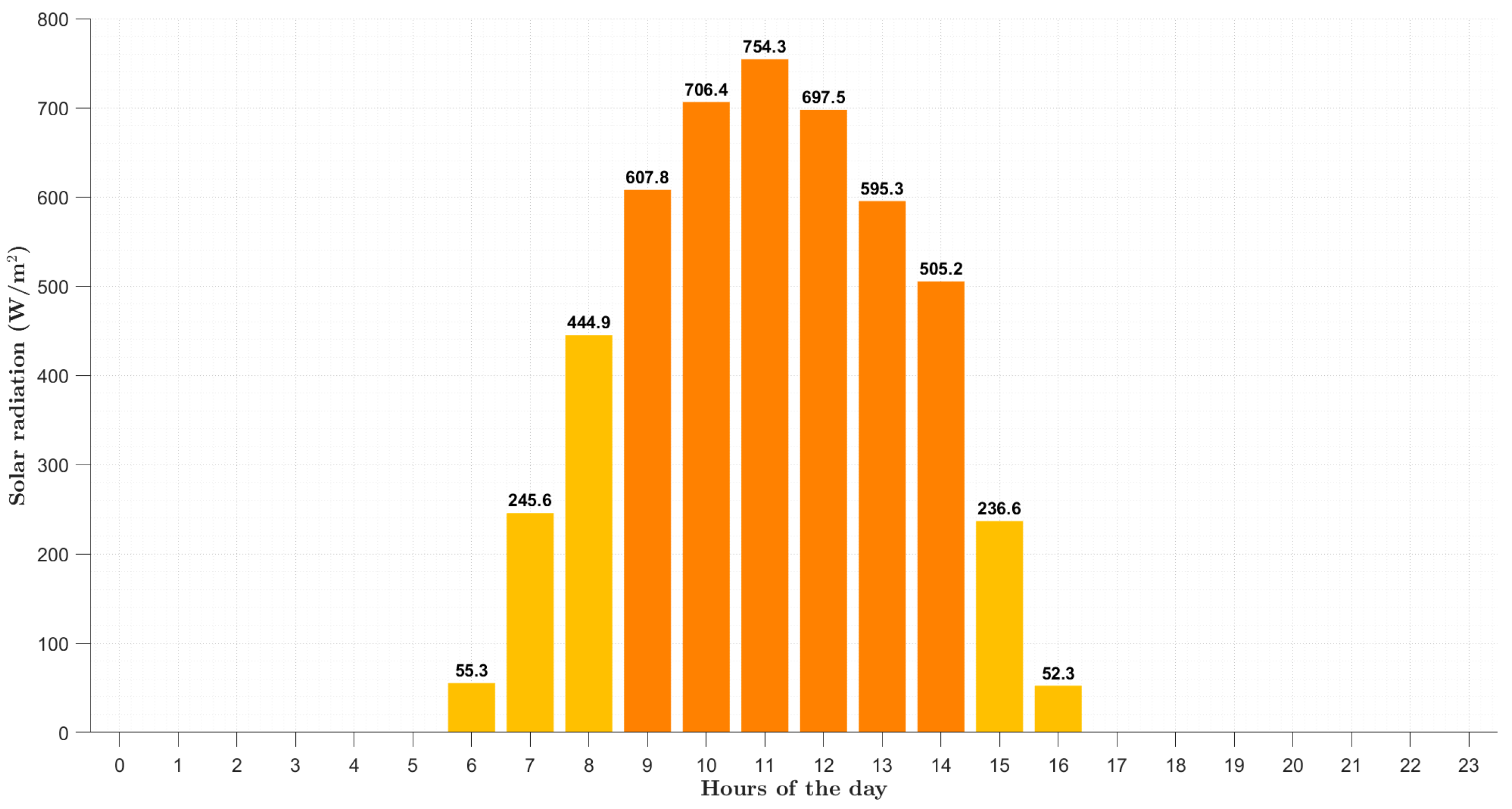
In parallel, the hourly solar radiation profile follows a typical bell-shaped distribution, as illustrated in Figure 3. The December average was selected as the representative case for low-irradiance periods. Analyzing this temporal behavior is essential for identifying peak energy generation intervals and establishing the system’s operational window [22].

The analysis of this curve allowed us to identify that, for the location of the case study, the interval of highest solar irradiation (>500 W/m²) is concentrated between 9:00 and 14:00, which is coincident with the monthly average solar radiation of 4.81 kW-hr/m²/day. This high productivity window is the period in which a direct pumping system (without electrical storage) reaches its maximum efficiency and flow rate [6], which allows us to define 4 h of operation. Similarly, research conducted under conditions analogous to this case study reported an equivalent 4 h period of operation [24].

Optimal Tilt Angle and Suitable Mounting Height of the Solar Panels

The determination of the optimal tilt angle and orientation is a typical problem in the design of photovoltaic systems, whose objective is to maximize solar irradiation throughout the day. The prevailing methodology, which remains a technical foundation, involves the integration of solar irradiation models with local data to optimize energy capture [25]. The impact of this methodology is such that it is employed in projects where more recent technologies are tested, as is the case with bifacial panels [26]. Despite the introduction of new variables by bifacial panels, the fundamental principles for calculating the optimal frontal angle, orientation, and analysis of global irradiation on inclined surfaces remain based on the same theoretical and procedural framework.

Table 3. Angle and inclination by base conditions (information from [25]).

Condition	Optimal Inclination	Explanation
Annual Average	19°	Equal to the latitude of Puebla.
Winter	29°	Latitude + 10° (19° + 10° = 29°). Maximizes energy capture in months with less sun.
Summer	9°	Latitude − 10° (19° − 10° = 9°). Maximizes energy capture in months with more sun.

presents the recommended seasonal inclinations for the case study location. However, to streamline operational management and ensure design robustness, the use of a fixed angle is recommended, thereby optimizing annual capture without the need for recurrent human manipulation.

It should be noted that, in the Northern Hemisphere, panels must be oriented toward the south to receive maximum irradiation throughout the day.

Well Data Provided by the Community

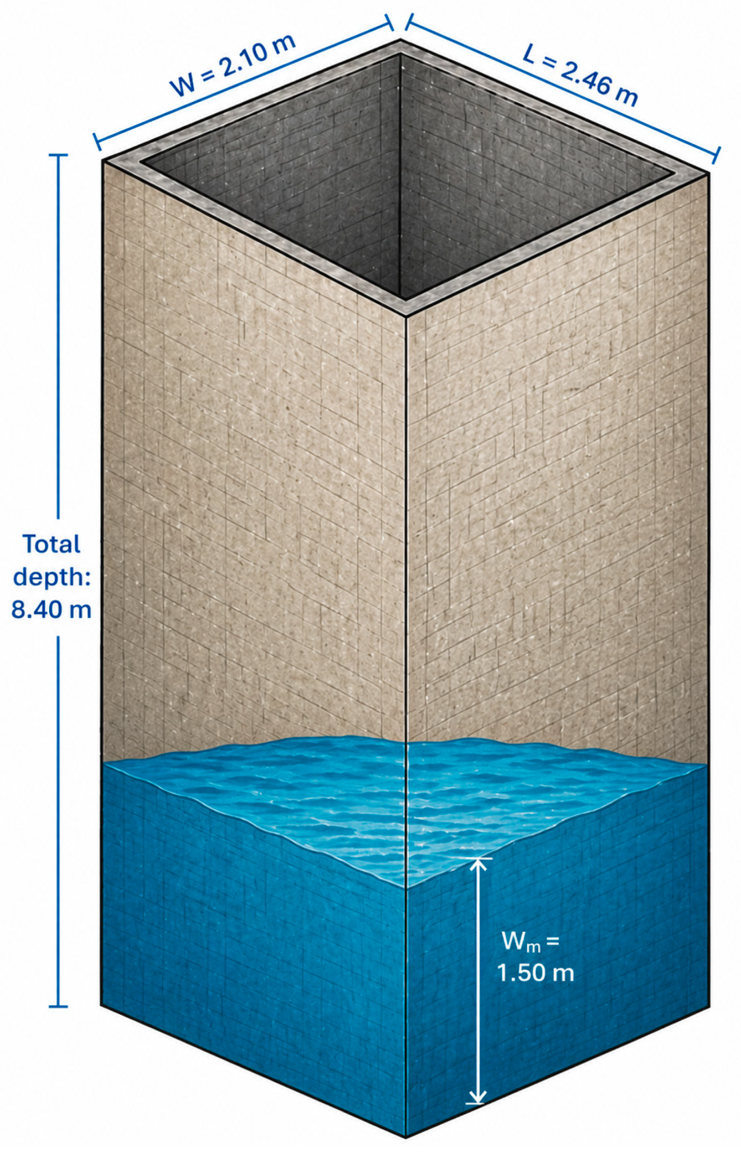
To size the solar pumping system, the characterization of the water source is required. For the case study, a well available in the community is used, which is presented with the following characteristics, illustrated in Figure 4.

In turn, the technical specifications are detailed in the following list:

• Internal dimensions: Width (W) × Length (L) = 2.10 m × 2.46 m.
• Total depth: 8.4 m.
• Thickness of the Water mirror (W_m) (available water column): 1.5 m.
• Natural recharge (T_r): Recharge amount (R_a) 0.2 m every 30 min.

With this data, the Volume of water (Vw) stored in the well was calculated, due to the existing relationship of width, length, and the water mirror given by the following Equation (1).

$${\mathit{V}}_w=\left(\mathit{W}\right)\left(\mathit{L}\right)\left({\mathit{W}}_{\mathit{m}}\right)=(\mathbf{2.10} \mathit{m})(\mathbf{2.46} \mathit{m})(\mathbf{1.5} \mathit{m})=\mathbf{7.749} {\mathit{m}}^{\mathbf{3}}$$

(1)

Similarly, the well recharge flow rate (Qr), with the relationship of the natural recharge:

$${\mathit{Q}}_{\mathit{r}}={\displaystyle \frac{\left(\mathit{W}\left)\right(\mathit{L}\right)\left({\mathit{R}}_{\mathit{a}}\right)}{{\mathit{T}}_{\mathit{r}}}}={\displaystyle \frac{\left(\mathbf{2.10} \mathit{m}\left)\right(\mathbf{2.46} \mathit{m}\right)(\mathbf{0.2} \mathit{m})}{\mathbf{0.5} \mathit{h}}}=\mathbf{2.066} {\mathit{m}}^{\mathbf{3}}/\mathit{h}$$

(2)

which is equivalent to a daily recharge flow rate (Q_d), assuming constant recovery over 24 h (Ro):

$${\mathit{Q}}_{\mathit{d}}=\left(\mathit{R}\mathit{o}\right)\left({\mathit{Q}}_{\mathit{r}}\right)=(\mathbf{24} \mathit{h})\left(\mathbf{2.066}{\displaystyle \frac{{\mathit{m}}^{\mathbf{3}}}{\mathit{h}}}\right)=\mathbf{49.58}{\displaystyle \frac{{\mathit{m}}^{\mathbf{3}}}{\mathit{d}\mathit{a}\mathit{y}}}$$

(3)

This natural recharge flow ensures continuous water availability, allowing sustainable extraction without affecting the static water level of the well. Previous studies, such as the evaluation of undersized systems in aquifers in Tanzania [11] and the study of tubed wells [27], have shown that inadequate system sizing can lead to overexploitation and eventual aquifer depletion. Therefore, proper sizing becomes a critical factor to ensure long-term sustainability. In this context, the available daily flow rate (50 m³/day) is a key parameter for determining the maximum crop area that can be irrigated without risking aquifer collapse.

2.1.2. Crop Selection (Step 2)

The implementation of the case study was contingent upon the determination of the most suitable crop, which was based on the essential criteria for the project’s viability.

• Regional Popularity: Crops with high demand and ease of sale in the area were prioritized.
• Environmental Compatibility: Species that demonstrated ease of cultivation and adaptability to the terrain were selected, considering the arid nature of the region.

The way in which the most popular crops in the area were identified was through the National Institute of Statistics and Geography (INEGI). This organization provided key information on the crops with the highest production and cultivated area in the region [28]. See

Table 4. Main crops and their productive relevance in the study area (2023).

Crop	Production (Tons)	Sown Area (Hectares)
White corn grain	512,143	512,656
Forage maize	233,474	10,209
Broccoli	128,680	9780
Onion	101,498	5858

.

In the realm of the second criterion (compatibility with the terrain), the options were further reduced using government reports. These reports specifically recommend the cultivation of corn, beans, and peanuts for their suitability and adaptation to the type of land being managed in the study area [29]. However, among these options, forage maize emerges as the most pertinent choice for various reasons:

• Short vegetative cycle: This presents minimum periods of 90 up to 150 days maximum, which allows adaptation to seasonality and enables up to 2 crop cycles annually with complementary irrigation [30].
• Proven compatibility in agrivoltaics systems: Research under this trend, being [31,32], shows that corn presents tolerance to partial shade when the panels are installed at 2 m height.
• Dual purpose: Forage maize has the capacity to produce forage which can be destined for animal feed apart from grain production, thus contributing to food security and sustainable development of the community.

Consequently, the choice of forage maize is supported through the popularity, the adaptability of the terrain, and in turn the technical evidence derived from the literature, which indicates to us its viability.

2.1.3. Calculation of Water Requirements (Step 3)

The water requirements of forage maize were calculated using the concept of evapotranspiration (ET), which integrates water loss through soil evaporation and plant transpiration. Therefore, to adjust these values to the specific conditions of the crop and its growth stage, the crop coefficient (Kc) is defined in the FAO-56 Manual [30].

For determining the water requirements of the project, the FAO’s CropWat 8.0 software was used. This specialized tool allows for the calculation of crop water requirements based on the integration of climatic data, specific characteristics of the selected crop, and soil properties.

Regarding meteorological data, the advantage was taken of the information requested by the software. The annual climatological data used for the study area (Mixteca Poblana) come from the reference [22], using the year 2022, as it is the closest to the date of the study.

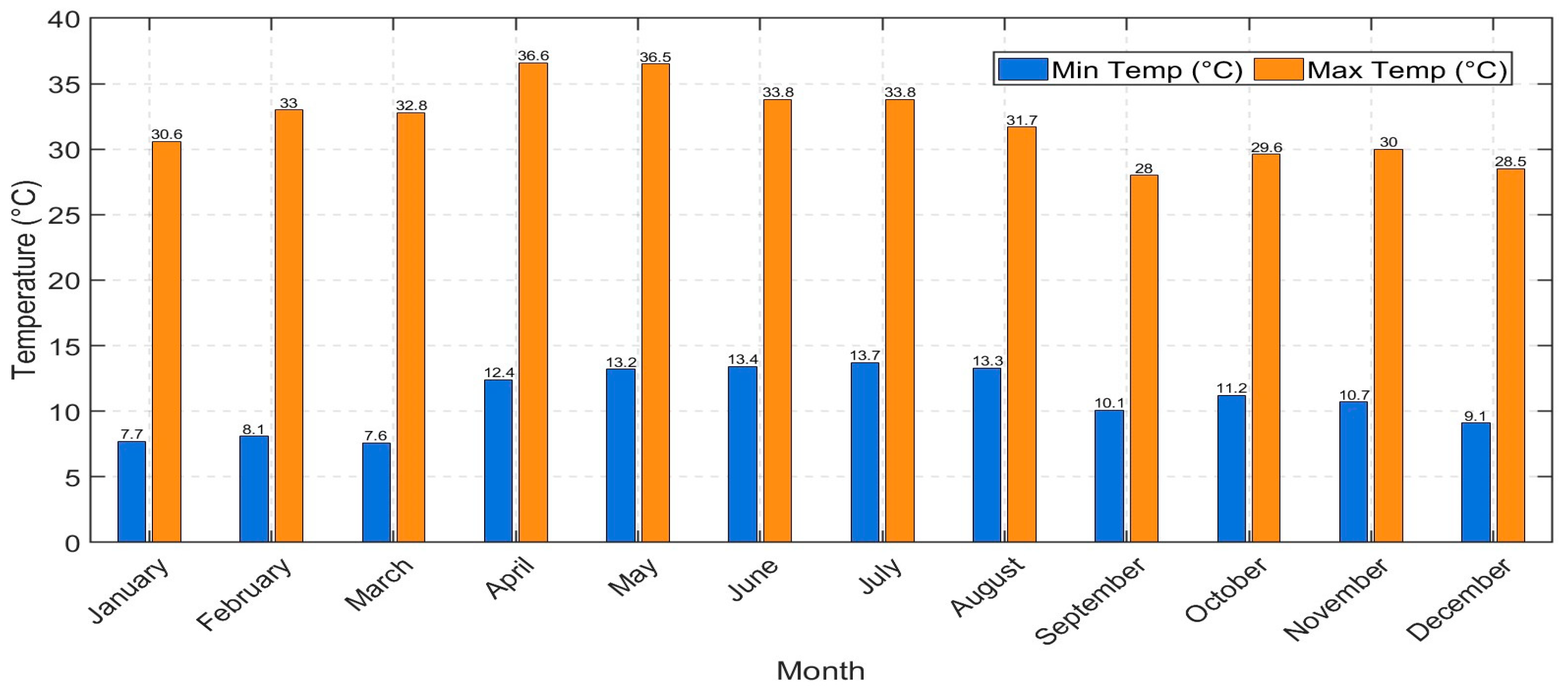
The first requirement of the software is the monthly maximum and minimum temperature data, which can be appreciated in Figure 5. Fundamental data, as it determines the reference evapotranspiration (ETO) through the Penman–Monteith equation, allows seeing the months with the highest irrigation requirement.

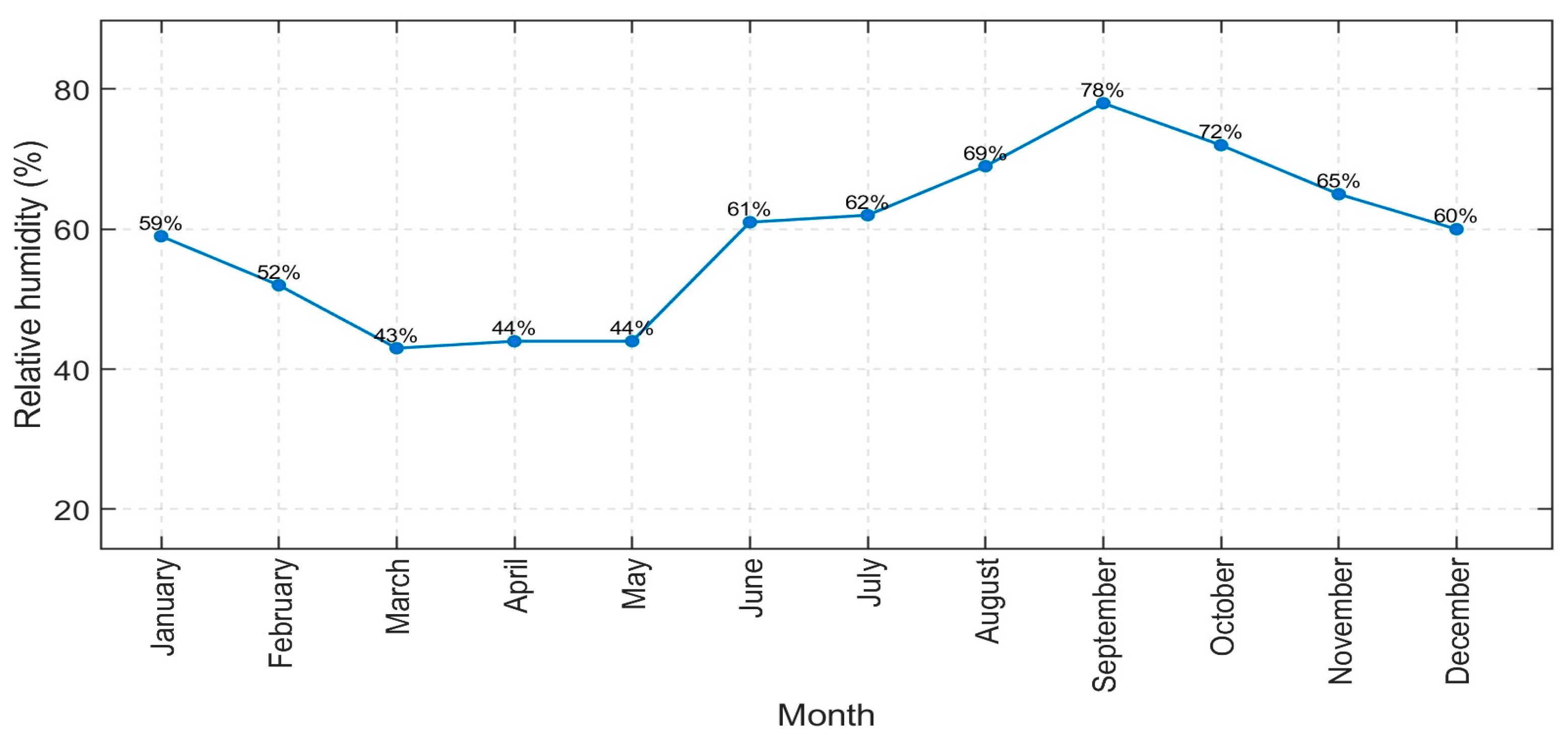
At the same time, the relative humidity data were compiled, which allows the software to see how it affects the transpiration rate: at a lower measure, greater water demand. These data can be seen in Figure 6.

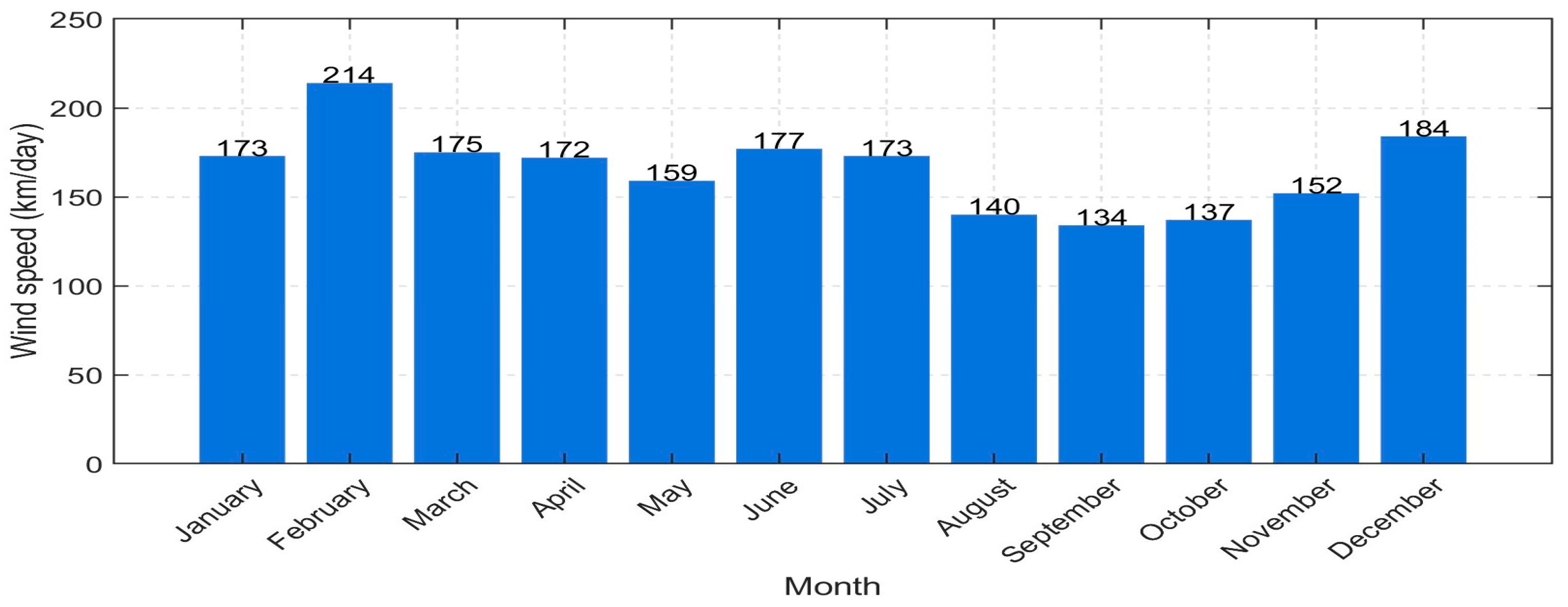
At the same time, the wind speed was investigated because this accelerates soil evaporation: to a greater extent, greater water loss. The data are seen in Figure 7.

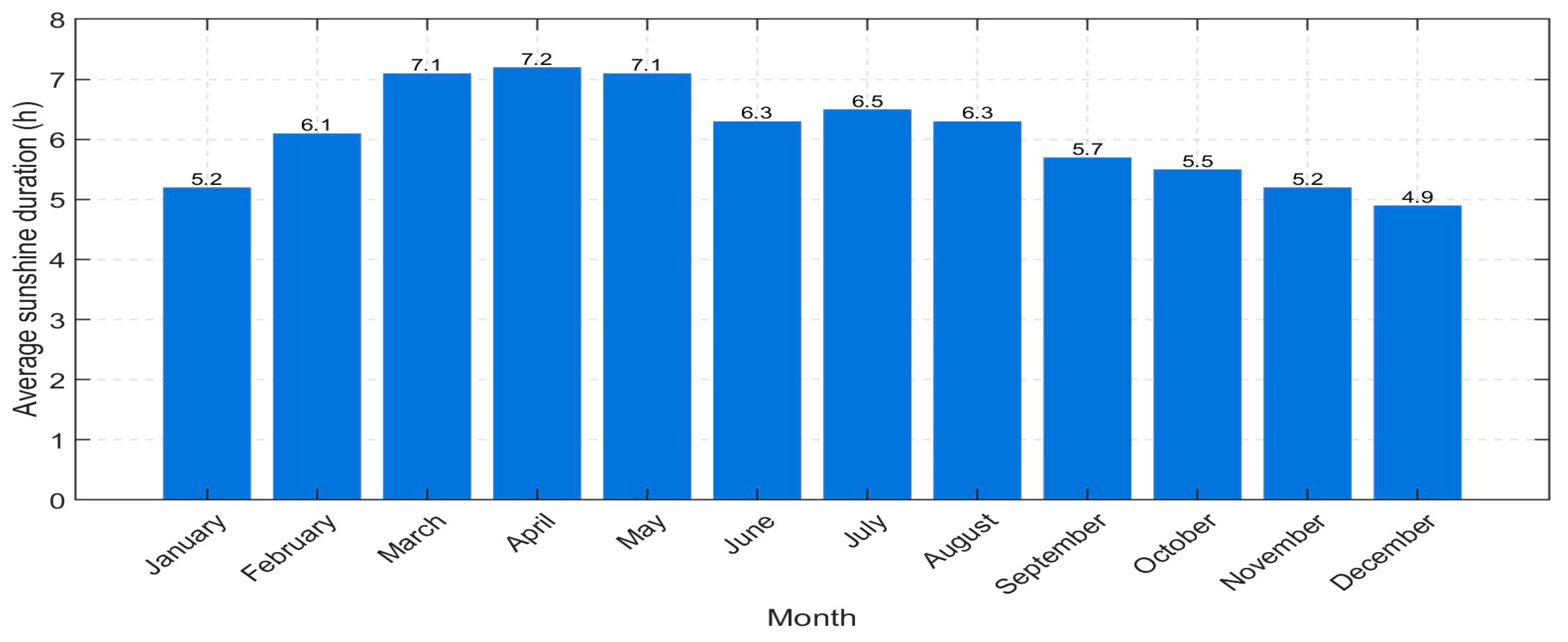
Being the next section to be investigated was apart from the hours of sunshine, since this data defines that at a greater measure, greater water demand. The compiled data are seen in Figure 8.

The compiled data were entered into the software to calculate the corresponding averages. Subsequently, radiation and evapotranspiration levels were determined; these resulting parameters are presented in

Table 5. Summary of characteristic climatic parameters of the case study.

Month	Temp Min (°C)	Temp Max (°C)	Humidity (%)	Wind (km/day)	Insulation (hours)	Rad (MJ/m2/day)	ETo (mm/day)
January	7.7	30.6	59	173	5.2	13.5	3.79
February	8.1	33	52	214	6.1	16.2	5.08
March	7.6	32.8	43	175	7.1	19.3	5.34
April	12.4	36.6	44	172	7.2	20.5	6
May	13.2	36.5	44	159	7.1	20.5	5.99
June	13.4	33.8	61	177	6.3	19.2	5.21
July	13.7	33.8	62	173	6.5	19.5	5.18
August	13.3	31.7	69	140	6.3	19.1	4.51
September	10.1	28	78	134	5.7	17.4	3.58
October	11.2	39.6	72	137	5.5	15.7	3.49
November	10.7	30	65	152	5.2	13.8	3.49
December	9.1	28.5	60	184	4.9	12.7	3.54
Average	10.9	32.1	59	166	6.1	17.3	4.6

.

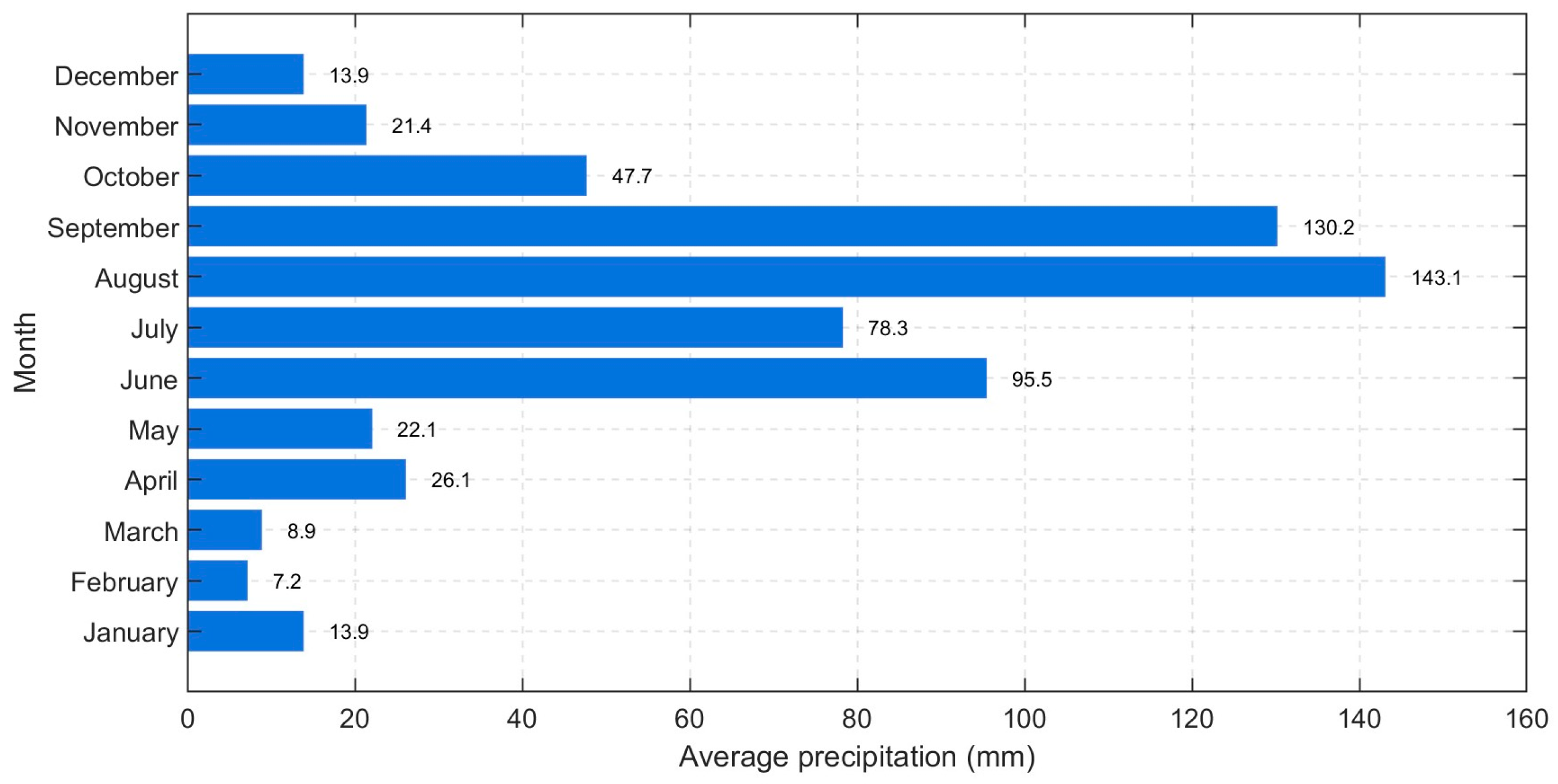
As the last fundamental climatological variable, rainfall (precipitation) is considered, representing the volume of water that falls on the ground, and which can be harnessed to reduce water demand. It is presented graphically in Figure 9.

The software also requires crop data, which consists of a series of key agroclimatic and phenological parameters. The corn cycle considered in this case study has a total duration of 140 days, which is divided into four phenological stages: initial (25 days), development (40 days), middle (45 days), and final (30 days), with durations established in accordance with the FAO-56 manual [30].

As mentioned above, the soil in the case study is arid, a condition that directly affects water demand. The planting date was established based on the ranges provided by INIFAP (Instituto Nacional de Investigaciones Forestales, Agrícolas y Pecuarias), which cover the period from March 15 to April 15 for better use of rainfall [33]. In this case study, the date was set for March 29 with harvesting on August 15.

In turn, the physical parameters considered for the water demand model used by the simulator and provided by the FAO-56 manual [30] are: The effective root depth, which physically represents how much water they can absorb, and monthly ETc (Actual Crop Evapotranspiration), which indicates the water consumed by the crop during that period. To calculate this demand, the crop coefficient (Kc) is used, a value that adjusts water demand according to the growth stage. Finally, the depletion factor (p) defines the crop’s tolerance to soil water deficit before experiencing stress. Response factors (f), with their associated averages, are used to assess how water stress impacts final crop yield. These parameters are grouped into

Table 6. Physical and agronomic parameters of forage maize according to FAO-56.

Parameter	Value
Effective Depth (m)	Initial: 1			Late season: 1.7
Monthly ETc	March: 8.92 mm			April: 9.27 mm
Crop Coefficient (Kc)	Initial: 0.7		Mid-season: 0.6		Late season: 0.9
Depletion Factor (p)	Initial: 0.55		Mid-season: 0.5		Late season: 0.6
Maximum Crop Height (m)	1.5 m
Response Factor (f)	Initial: 1	Development: 1.3	Mid-season: 1.6	Late-season:1.3	Average: 1.25

.

Finally, soil data are required since site characterization studies can take years. Instead, the values recommended by the FAO-56 manual were used [30]. These are presented in

Table 7. Estimated soil characterization under FAO-56 manual recommendations [30].

Parameter	Value in the Study	Irrigation Implication
Field Capacity (FC)	120 mm/m	Defines the upper limit of available water for the roots.
Maximum Infiltration	25 mm/day	Establishes the maximum water application rate without generating runoff.
Rooting Depth	120 cm	Determines the active water absorption zone, linked to the effective soil depth.
Critical Depletion	55% (0.55)	The irrigation threshold was set at 55%, the maximum value of the technical range (40–55%), as it represents the point of greatest water stress and criticality for the system.

for the type of soil available, which directly influences the crop’s water balance by conditioning both the soil’s water retention capacity and the fraction of water effectively available to the plant. The parameters determine the crop’s water demand and the maximum irrigation threshold without affecting its development.

The results obtained through CropWat 8.0 (

Table 8. Water requirements for the first crop cycle.

Month	Decade (10 Days)	Stage	Kc	ETc (mm/day)	ETc (mm/dec)	Eff. Precip. (mm/dec)	Irrig. Req. (mm/dec)
Mar	3	Initial	0.7	3.89	7.8	0.8	7.8
Apr	1	Initial	0.7	4.05	40.5	7.1	33.3
Apr	2	Initial	0.7	4.2	42	9.2	32.8
Apr	3	Development	0.7	4.18	41.8	8.5	33.2
May	1	Development	0.68	4.1	41	5.5	35.5
May	2	Development	0.67	4.03	40.3	4.2	36.1
May	3	Development	0.66	3.78	41.6	11.8	29.8
Jun	1	Medium	0.65	3.56	35.6	22.6	13
Jun	2	Medium	0.65	3.39	33.9	30.4	3.6
Jun	3	Medium	0.65	3.39	33.9	27.9	6
Jul	1	Medium	0.65	3.38	33.8	22.5	11.3
Jul	2	Final	0.74	3.82	38.2	20.3	17.9
Jul	3	Final	0.94	4.65	51.1	25.8	25.3
Aug	1	Final	0.94	4.44	44.4	33.7	10.7
Aug	2	Final	0.94	4.23	25.4	23.4	5.8
Total					551.1	253.7	302.1

) in this quantifies the water requirements of forage maize throughout the crop cycle. These specific requirements must be met by the pumping system; these values then serve as a baseline to estimate the requirements for the second crop cycle.

For the analyzed crops, which require a total water volume of 302.1 mm per decade (10 days) under local climatic and soil conditions, and for conversion to volumetric units per hectare (ha), the standard relationship is applied, as shown in Equation (4).

$$\mathbf{1} \mathit{m}\mathit{m}=\mathbf{10}{\displaystyle \frac{{\mathit{m}}^{\mathbf{3}}}{\mathit{h}\mathit{a}}}$$

(4)

For the calculation of the global water requirement (QWR), the following Equation (5) is used:

$$\mathit{Q}\mathit{W}\mathit{R}=\left(\mathbf{302.1}\right)\left(\mathbf{10} {\displaystyle \frac{{\mathit{m}}^{\mathbf{3}}}{\mathit{h}\mathit{a}}}\right)=\mathbf{3021}{\displaystyle \frac{{\mathit{m}}^{\mathbf{3}}}{\mathit{h}\mathit{a}}}$$

(5)

The net daily water requirement (V_req) is obtained by distributing this total volume over the growth cycle, resulting in 21.58 m³/day per hectare.

For this case, the study is being sized under the gravity irrigation technique, which is widely used for its low cost and ease of implementation and presents an efficiency (η_irrig) of 50% [30], This implies that only half of the applied water is effectively utilized by the crop, requiring an additional volume (V_add) to compensate for losses, as defined in Equation (6):

$${\mathit{V}}_{\mathit{a}\mathit{d}\mathit{d}}={\displaystyle \frac{\left({\mathit{V}}_{\mathit{r}\mathit{e}\mathit{q}}\right)}{{\mathit{\eta }}_{\mathit{i}\mathit{r}\mathit{r}\mathit{i}\mathit{g}}}}={\displaystyle \frac{\left(\mathbf{21.58}\frac{{\mathit{m}}^{\mathbf{3}}}{\mathit{d}\mathit{a}\mathit{y}}\right)}{\mathbf{0.5}}}=\mathbf{43.16}{\displaystyle \frac{{\mathit{m}}^{\mathbf{3}}}{\mathit{d}\mathit{a}\mathit{y}}}$$

(6)

With these parameters, the area of land that the well can cover without suffering water stress, the maximum area (M_a), using Equation (7).

$${\mathit{M}}_{\mathit{a}}={\displaystyle \frac{{\mathit{Q}}_{\mathit{d}}}{{\mathit{V}}_{\mathit{a}\mathit{d}\mathit{d}}}}={\displaystyle \frac{\mathbf{49.58}\frac{{\mathit{m}}^{\mathbf{3}}}{\mathit{d}\mathit{a}\mathit{y}}}{\mathbf{43.16}\frac{{\mathit{m}}^{\mathbf{3}}}{\mathit{d}\mathit{a}\mathit{y}·\mathit{h}\mathit{a}}}}=\mathbf{1.15} \mathit{h}\mathit{a}$$

(7)

For safety reasons, it was reduced to one hectare to leave a margin of error. Since the literature only indicates the possibility of two maize crop cycles, but does not specify a calendar of dates, it was necessary to perform an iterative analysis within the modeling software. This interaction process sought to establish the optimal dates for the second crop cycle under two fundamental criteria:

• Not to interfere with the calendar of the first crop cycle.
• To make the most of the available natural precipitation to reduce artificial irrigation.

The final dates and the parameters resulting from this optimization are detailed in

Table 9. Simulations of scenarios for the start of the second crop cycle using CROPWAT to minimize water requirements.

Sowing Date	Total ETc (mm)	Effective Precipitation (mm)	Required Irrigation (mm)
September	377	133.7	258.7
October	425.1	71.3	357.9
November	473.5	54.9	421.1

.

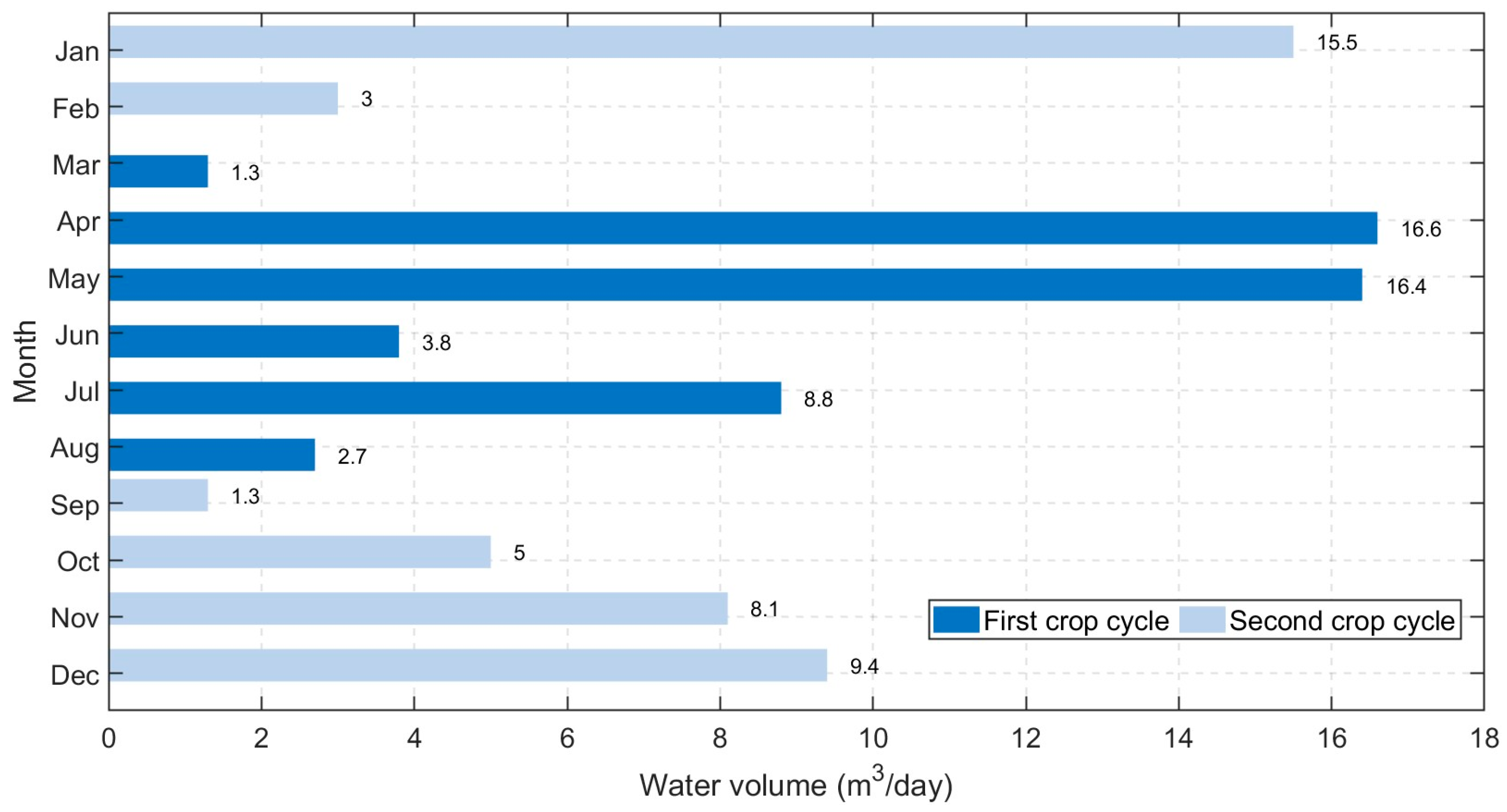
The selected cycle spans from September 19 to February 6, taking advantage of greater rainfall to reduce water needs. The annual combination of both cycles is illustrated in Figure 10.

These monthly values represent the average daily water demand that must be met in each month of the year.

2.1.4. Determination of Pump Power (Step 4)

The selection of the pumping unit is fundamental to guaranteeing water security and system reliability in agricultural contexts. In this study, the sizing is based on the maximum daily demand (D_max) of 16.6 m³/day. Following the methodology for daily operating hours with a safety margin (Top = 4 h), the required flow rate (Q_req) is calculated as follows, determined by Equation (8):

$${\mathit{Q}}_{\mathit{r}\mathit{e}\mathit{q}}={\displaystyle \frac{{\mathit{D}}_{\mathit{m}\mathit{a}\mathit{x}}}{{\mathit{T}}_{\mathit{o}\mathit{p}}}}={\displaystyle \frac{\mathbf{16.6} \frac{{\mathit{m}}^{\mathbf{3}}}{\mathit{d}\mathit{a}\mathit{y}}}{\mathbf{4} \mathit{h}}}=\mathbf{4.15}{\displaystyle \frac{{\mathit{m}}^{\mathbf{3}}}{\mathit{h}}}=\mathbf{69.2}{\displaystyle \frac{\mathit{L}}{\mathit{m}\mathit{i}\mathit{n}}}=\mathbf{0.00115}{\displaystyle \frac{{\mathit{m}}^{\mathbf{3}}}{\mathit{s}}}$$

(8)

To calculate the hydraulic power (P_h), a Total Dynamic Head (TDH) of 13 m was established, accounting for the well depth (8 m), water table height (1.5 m), and the additional 6 m required for gravity irrigation. Using the density of water (p = 1000 kg/m³) and gravity (g = 9.81 m/s²), and applying an efficiency factor (η_p) of 0.5 based on standard performance benchmarks for motor pumps, the power is derived as follows:

$${\mathit{P}}_{\mathit{h}}={\displaystyle \frac{{(\mathit{Q}}_{\mathit{r}\mathit{e}\mathit{q}}\left)\right(\mathit{T}\mathit{D}\mathit{H}\left)\right(\mathit{p}\left)\right(\mathit{g})}{{\mathit{n}}_{\mathit{p}}}}={\displaystyle \frac{\left(\mathbf{0.00115}\frac{{\mathit{m}}^{\mathbf{3}}}{\mathit{s}}\right)(\mathbf{13} \mathit{m})(\mathbf{1000} \mathit{k}\mathit{g}/{\mathit{m}}^{\mathbf{3}})(\mathbf{9.81} \mathit{m}/{\mathit{s}}^{\mathbf{2}})}{\mathbf{0.5}}}=\mathbf{294} \mathit{W}$$

(9)

To ensure operational stability and provide a robust safety factor against mechanical wear and solar variability, a 1 hp (746 W) pump was selected. This selection avoids excessive oversizing while maintaining the motor within its optimal performance curve, following the safety factor criteria recommended by [34].

2.1.5. Calculation of Required Energy (Step 5)

The sizing of the photovoltaic system is based on the total energy required to meet the pumping demand, accounting for inherent system losses and local solar availability. The hydraulic energy (H_energy) needed to lift the target water volume is determined through the fundamental potential energy Equation (10). For this calculation, the operational time (T_op) is converted to seconds (17 280 s)

$$\begin{gathered} {\mathit{H}}_{\mathit{e}\mathit{n}\mathit{e}\mathit{r}\mathit{g}\mathit{y}}=\left(\mathit{P}\right)\left(\mathit{g}\right){(\mathit{Q}}_{\mathit{r}\mathit{e}\mathit{q}}\left)\right(\mathit{T}\mathit{D}\mathit{H}\left)\right({\mathit{T}}_{\mathit{o}\mathit{p}})= \\ \left(\mathbf{1000}{\displaystyle \frac{\mathit{k}\mathit{g}}{{\mathit{m}}^{\mathbf{3}}}}\right)\left(\mathbf{9.81}{\displaystyle \frac{\mathit{m}}{{\mathit{s}}^{\mathbf{2}}}}\right)\left(\mathbf{0.00115}{\displaystyle \frac{{\mathit{m}}^{\mathbf{3}}}{\mathit{s}}}\right)\left(\mathbf{13} \mathit{m}\right)\left(\mathbf{17\; 280} \mathit{s}\right)=\mathbf{2,533\; 975} \mathit{J}=\mathbf{704} \mathit{W}\mathit{h} \end{gathered}$$

(10)

Considering the overall losses associated with the pump, energy conversion (inverter), and energy transport (controller), these are estimated to range from 40% to 60% for low-power photovoltaic pumping systems, choosing the midpoint between the two at 50% (η_global) [35]. The daily electrical energy required (E_req) is shown in Equation (11).

$${\mathit{E}}_{\mathit{r}\mathit{e}\mathit{q}}={\displaystyle \frac{{\mathit{H}}_{\mathit{e}\mathit{n}\mathit{e}\mathit{r}\mathit{g}\mathit{y}}}{{\mathit{\eta }}_{\mathit{g}\mathit{l}\mathit{o}\mathit{b}\mathit{a}\mathit{l}}}}={\displaystyle \frac{\mathbf{704} \mathit{W}\mathit{h}}{\mathbf{0.5}}}=\mathbf{1408} \mathit{W}\mathit{h}/\mathit{d}\mathit{a}\mathit{y}$$

(11)

To satisfy this daily demand, a photovoltaic array of 3 panels of 150 W (450 Wp total) is proposed. This configuration is specifically selected following the technical recommendations in [36] for systems utilizing lithium-ion battery storage, which are effective for managing current peaks during pump startup. The solar energy generated (E_gen) relates to the peak power of the array (P_A), the peak sun hours (PSH) obtained in Table 2, which used the lowest data (December), and a generation efficiency factor (η), since these include losses due to temperature, dirt, inverter efficiency, and other factors. Typically, generation efficiency is between 0.70 and 0.85, and the lowest value, 0.7, was chosen (η_generation).

$${\mathit{E}}_{\mathit{g}\mathit{e}\mathit{n}}=\left({\mathit{P}}_A\right)\left(\mathit{P}\mathit{S}\mathit{H}\right)\left({\mathit{\eta }}_{\mathit{g}\mathit{e}\mathit{n}\mathit{e}\mathit{r}\mathit{a}\mathit{t}\mathit{i}\mathit{o}\mathit{n}}\right)=(\mathbf{450} \mathit{W})(\mathbf{4.81} \mathit{h})\left(\mathbf{0.7}\right)=\mathbf{1515} \mathit{W}\mathit{h}/\mathit{d}\mathit{a}\mathit{y}$$

(12)

The solar generation (1515 Wh/day) exceeds the demand (1408 Wh/day), guaranteeing a safety margin of 7.6%. This surplus ensures system autonomy even on days of reduced radiation. Furthermore, empirical evidence from similar research in the region [37] demonstrates that 450 W arrays with Li-ion storage can effectively cover the energy demand of 1 hp pumps in intermittent operation, validating the technical feasibility of this sizing.

Up to this stage, the pumping system design adheres to the procedures defined in the base methodology. Based on the obtained design parameters, methodological extension is subsequently developed, with the objective of establishing a technical correlation among these parameters to support component dimensioning and selection.

In this context, it is important to distinguish the role of each stage. The general methodology (Section 2.1) defines the system requirements, including water demand, energy needs, and hydraulic constraints, providing a theoretical sizing framework. In contrast, the extension presented in Section 2.2 focuses on the practical implementation of these requirements through the selection and integration of commercially available components. Therefore, while the base methodology determines what the system requires, extension defines how these requirements are physically realized.

2.2. Extension of the Methodology: Technical Study (Step 6)

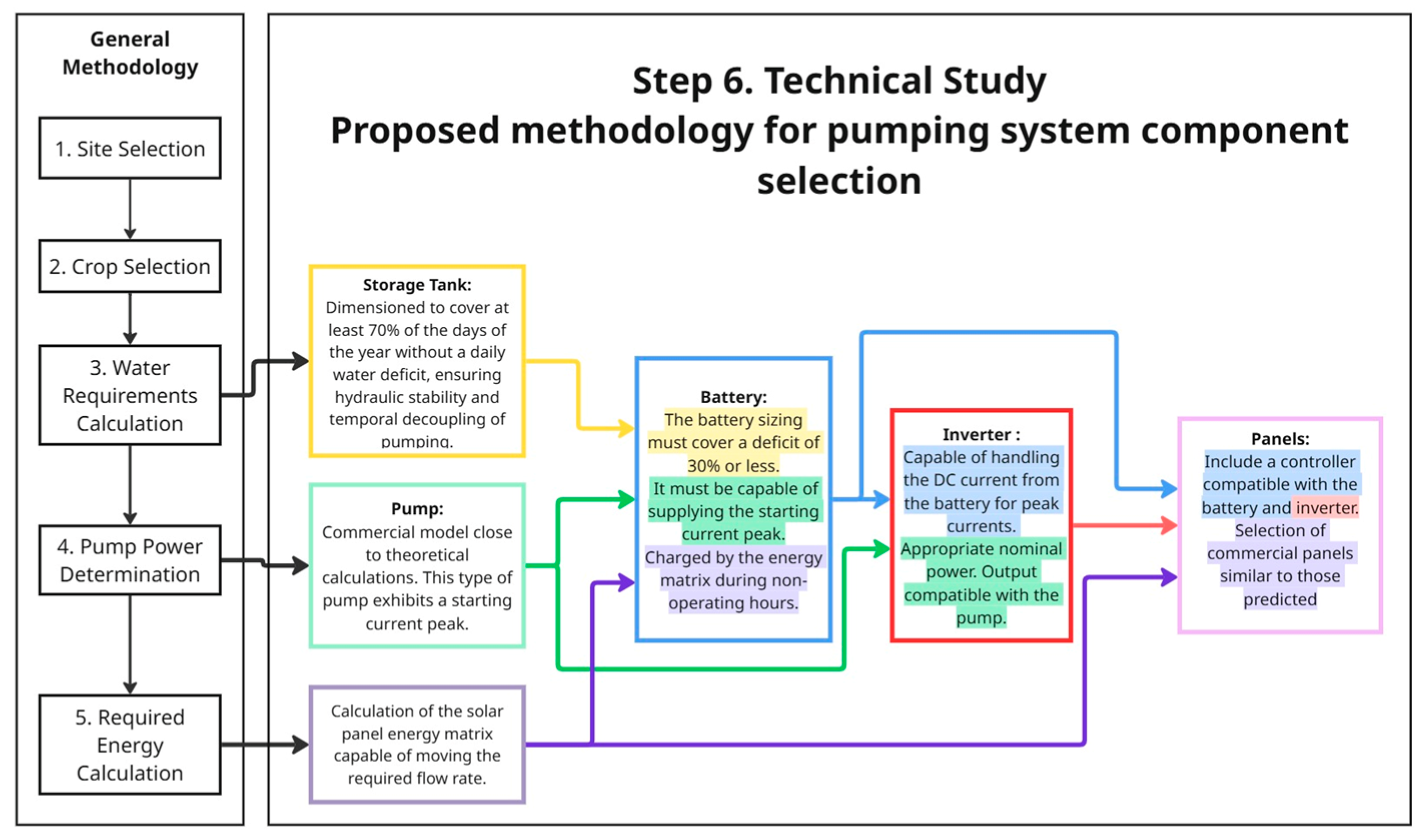
This section presents the primary contribution of the study: a structured extension of the base methodology, focused on the integrated and technically consistent selection of system components for the construction of the pumping system. The proposed extension builds directly upon the preceding design stages, where Steps 1–2 define the initial design conditions and Steps 3–5 establish the primary hydraulic and electrical constraints. The overall structure of the proposed extension is illustrated in Figure 2.

2.2.1. Hydraulic Integration and System Autonomy

First, the technical requirements of the system are established based on the basic methodology, with steps 3 to 5 defining the requirements for the commercial components.

Now that the requirements have been established, a parallel choice is made due to the importance of both components: the storage tank and the pump, as they are the most expensive components and the central element of the system, respectively.

Storage Tank

The selection of commercial storage tanks is based on a daily water balance analysis. Proper sizing is critical; inadequate capacity compromises operational stability beyond mere construction costs. Consequently, the elevated tank acts as a strategic buffer, decoupling water availability from solar intermittency and ensuring a resilient supply for irrigation.

The proposed selection criterion focuses on annual coverage: the percentage of days per year where the tank capacity fully meets daily water demand without a deficit. A minimum coverage of 70% is recommended to ensure stable operation throughout most of the year.

Based on the project’s overall water requirements, a 12 m³ tank is proposed, providing 75% annual autonomy, as shown in

Table 10. Hydraulic autonomy provided by a 12 m³ storage tank.

Month	Average Daily Water Requirement (m3/day)	Daily Balance with Respect to Tank (m3)
Jan	15.5	−3.5
Feb	3	+9
Mar	1.3	+10.7
Apr	16.6	−4.6
May	16.4	−4.4
Jun	3.8	+8.2
Jul	8.8	+3.2
Aug	2.7	+9.3
Sep	1.3	+10.7
Oct	5	+7
Nov	8.1	+3.9
Dec	9.4	+2.6

. This capacity was determined by identifying the days without a water deficit. The system covers approximately 273 days, with deficits occurring only in January, April, and May. This sizing ensures hydraulic stability for most of the annual period.

The daily water deficits identified through this analysis form the basis for the subsequent sizing of the battery, which must be capable of covering the daily deficits.

Pump

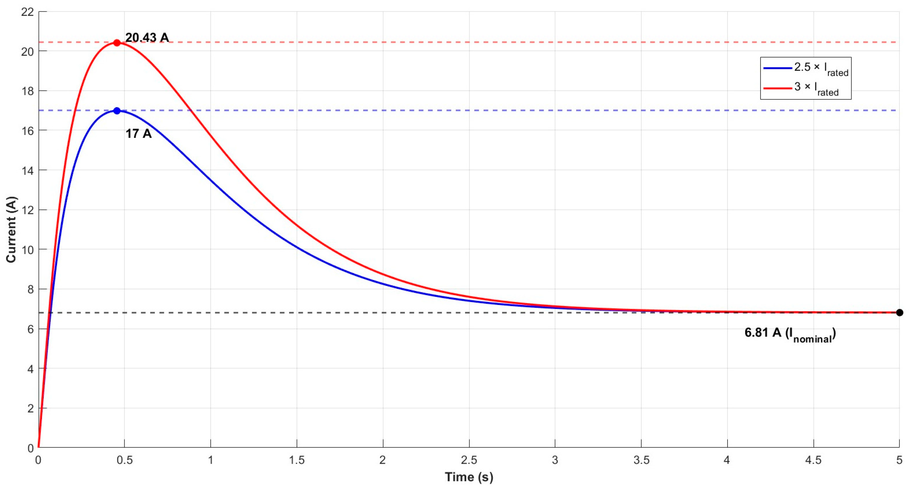
The selection of the pump also corresponds to the initial requirements of the system. The choice is made based on the power and flow rate calculated in step 4. The closest to these calculations is a 1 hp submersible centrifugal pump with a flow rate of 70 L/min, which has a peak current at start-up that, thanks to a safety factor of 2.5 to 3 times the nominal current of the pump (6.81 A), according to studies characterizing this type of pump, is determined to be a maximum peak of 20.43 A [38], with a duration of less than 0.5–1 s. However, for sizing purposes, this interval was adopted as a design limit condition to evaluate the maximum instantaneous power demand during system startup. A representation of this peak at startup in the Hyundai pump can be seen in Figure 11.

To handle this current peak, the use of batteries is a suitable alternative, as they offer instant power during start-up [39], autonomy, and better response to current peaks. Given that the battery must be capable of providing this current peak, this must be considered when sizing the battery.

In addition, the selected pump has technical operating characteristics of 110 V at a frequency of 60 Hz, which is essential information for selecting the inverter.

2.2.2. Sizing of the Energy Storage System

Given the incorporation of a storage tank within the proposal to address the daily water balance, the battery system is meticulously sized to address the identified energy deficits and peak operating demands. Additionally, the system’s configuration enables the battery to supply the requisite energy during pump startup, thereby delivering the maximum current. Furthermore, the battery’s discharge capacity is engineered to be recharged in a shorter duration than the operating hours.

Battery

This stage defines the battery capacity required to bridge the storage tank’s water deficit (25%) while managing pump startup peaks. The sizing ensures that the battery can recharge within the established operating window to maintain system autonomy.

While literature [40] suggests that a 12 V, 75 Ah battery suffices for low-horsepower centrifugal pumps, the increased energy demands of this system require greater capacity. A larger storage bank extends autonomy during low solar irradiance, ensuring continuous operation. Consequently, a 12 V, 200 Ah configuration was selected, providing 2400 Wh of total energy. To preserve service life, the Depth of Discharge (DoD) is limited to 80%, resulting in 1920 Wh of usable energy.

Based on these precedents, a 12 V and 200 Ah configuration is considered as the first option, which provides 2400 Wh of usable energy. To verify autonomy and ensure service life, the depth of discharge (DoD) will be limited to a maximum of 80%, giving 1920 Wh of usable energy.

Cover the Deficit

For this stage of the sizing process, the month with the highest water deficit is analyzed, which corresponds to April with a maximum deficit volume (V_def) of 4 600 L. Considering the nominal pump flow rate (Q_p) of 70 L/min, the required operating time (t_op) to cover this deficit in the worst-case scenario is calculated using Equation (13):

$${\mathit{t}}_{\mathit{o}\mathit{p}}={\displaystyle \frac{{\mathit{V}}_{\mathit{d}\mathit{e}\mathit{f}}}{{\mathit{Q}}_{\mathit{p}}}}={\displaystyle \frac{\mathbf{4\; 600} \mathit{L}}{\mathbf{70}\frac{\mathit{L}}{\mathit{m}\mathit{i}\mathit{n}}}}=\mathbf{66} \mathit{m}\mathit{i}\mathit{n}$$

(13)

Returning to Equation (11) with the set time of 66 min, 326 W of hydraulic energy is required, which means that the energy used to cover the deficit is approximately 17% of the usable battery, which maintains the initial rating of 12 V with 200 Ah.

Current Peak

Given the peak current of 20.43 A at the output of 110 V pump, an AC starting power of 2247 W is obtained. Assuming a 70% efficiency rating for the generation components, the battery must deliver a DC power output of 3210 watts.

It is imperative to note that, at a voltage of 12 V, this power requires a DC of 267.5 A. The 12 V LifePO4 orgophy battery with 200 Ah has the capacity to supply 400 A, making it a suitable choice for providing the starting peak. Concurrently, the 267.5 A and 3210 W will satisfy the initial criterion of the third system requirement.

At a voltage of 12 V, this power requires a DC of 267.5 A. The 12 V LifePO4 orgogpy battery with 200 Ah can supply 400 A, making it a suitable choice for providing the starting peak. Meanwhile, the 267.5 A and 3210 W will fulfill the first point in the third system requirement.

Battery Charges

This calculation considers the daily energy provided by the system in December (E_gen = 1515 Wh) from Equation (12), which, using Equation (14), is converted to the average power (P_avg) of the system with the minimum radiation in the case study (PSH)

$${\mathit{P}}_{\mathit{a}\mathit{v}\mathit{g}}={\displaystyle \frac{{\mathit{E}}_{\mathit{g}\mathit{e}\mathit{n}}}{\mathrm{P}\mathrm{S}\mathrm{H}}}={\displaystyle \frac{\mathbf{1\; 515} \mathit{W}\mathit{h}}{\mathbf{4.81} \mathit{h}}}=\mathbf{315} \mathit{W}$$

(14)

The energy required to cover the water deficit (E_def) corresponds to 326 Wh, which is equivalent to 17% of the battery’s usable energy. The charging time (Tc) is calculated using Equation (15):

$${\mathit{C}}_{\mathit{t}}={\displaystyle \frac{{\mathit{E}}_{\mathit{d}\mathit{e}\mathit{f}}}{{\mathit{P}}_{\mathit{a}\mathit{v}\mathit{g}}}}={\displaystyle \frac{\mathbf{326} \mathit{W}\mathit{h}}{\mathbf{315} \mathit{W}}}=\mathbf{1.04} \mathit{h}$$

(15)

This finding suggests that the system can recuperate the energy expended within approximately one hour of operation under minimal radiation conditions. This finding suggests that the selection and sizing of the battery were appropriate, in accordance with the criteria established for the battery type.

2.2.3. Validation of Electrical Compatibility and System Start-Up Capability

Due to the need to convert energy when choosing an AC pump to adapt the energy provided by the DC panels and the battery, an inverter is required that can support the requirements of both the pump at its output and the battery at its input.

Inverter

Since the system requires a starting current of 267.5 A from the battery, it is imperative to use equipment that exceeds this threshold to avoid overload shutdowns. After analysis, the Energizer ENK4000 inverter was selected, which guarantees operational continuity by offering DC support at startup of up to 350 A. In addition, this model ensures the integrity of the pump motor by providing a rated power of 4000 W (exceeding the 3210 W required) and an inverter output of 110 V/60 Hz, strictly complying with the established electrical parameters.

2.2.4. Photovoltaic System Selection and Compatibility

The part that will power the project includes voltage adjustment by a solar controller capable of supporting the battery current and compatible with the inverter input, along with specialized commercial panels for irrigation that are easily accessible in the country.

Inclusion of a Battery-Compatible Controller and Inverter

The solar controller that must be selected must be compatible with the 12 V and 200 Ah LiFePO4 battery bank, have an operating voltage range in direct current in accordance with 12 V systems (maximum input voltage from the photovoltaic array not less than 60 V DC), and be capable of managing a minimum power of 450 W. It must also allow integration into a common DC bus with a 4000 W inverter, considering high transient currents of around 267.5 A in the system. The controller must incorporate internal and external electrical protections, including a protection fuse on the DC side with a minimum capacity of 300 A, as well as overload and overvoltage protection functions, ensuring safe and stable operation of the system.

Selection of Similar Commercial Panels

Given that the system is intended to operate in a rural and isolated environment, the selection of solar panels must prioritize commercial availability, ease of replacement, and resistance to adverse environmental conditions. Although the annual degradation of the modules is low, they are exposed to external risks that may require unscheduled replacements. For this reason, commercial solar panels with characteristics equivalent to those specified in the design are selected, giving preference to models with high availability in the domestic market, robust design, and certifications for applications in rural and agricultural areas. In this context, the EPCOM PRO-15012 panel in its polycrystalline version is considered, designed for irrigation applications and directly compatible with load control and regulation systems.

System Design Summary and Economic Assessment

The following section summarizes the final component selection obtained from the proposed methodological development presents the technical and economic characteristics of the selected components, integrating the results of the previous design and sizing stages.

Table 11. Selected components for the case study.

Component	Technical Specifications	Cost $ (MXN)
Storage tank	12,000 L capacity in high-density polyethylene (HDPE). Dimensions: 3.25 m (height) × 2.45 m (diameter). Brand: Disomex.	$33,000.00
1 hp pump	Power of 1 hp (750 W) with a flow rate of 70 L/min. Designed for well extraction. Brand: Hyundai.	$2690.00
12 V 200 Ah LiFePO4 battery	LiFePO4 technology (12 V, 200 Ah) with integrated BMS system. Maximum discharge current: 200 A. Brand: Orgogpy.	$10,700.00
Inverter	Nominal power 4000 W. Output: 110 V/60 Hz. Supports 350 A. Brand: Energizer 4000.	$16,536.00
3 × 150 W solar panels	Brand EPCOM pro15012 Maximum power 150 W, Maximum voltage 18.3 V, Maximum amperage 8.2 A	$5928.00
Panel structure	Stainless steel. Area: 2.01 m × 1.47 m. Inclination: 19°.	$2684.00
Plumbing	1 1/4″ PVC pipe with a length of 13 m; designed to cover a Total Dynamic Head (TDH) compatible with the pump output.	$5750.00
Total		$89,734.00

presents the technical and economic characteristics of the selected components, integrating the results of the previous design and sizing stages.

Based on this sizing, a financial feasibility analysis was conducted, considering the system’s performance in agricultural irrigation. Annual revenue was estimated based on a yield of 7.5 t/ha [41], and a price of $6278 MXN/t, resulting in a gross profit of $94,168 MXN per year (accounting for two growing cycles). On the other hand, the annual production cost was estimated at $21,548 MXN ($10,774 MXN/ha per cycle), based on recent industry data that includes land preparation, fertilization, seed, pest control, harvesting, and transportation [42].

The total initial investment was estimated at $111,274.82 MXN, a figure that includes the cost of the pumping equipment and the first year’s operating costs. Starting in the second year, two preventive maintenance sessions were planned, at an annual cost of $6000 MXN. The resulting cash flow is shown in

Table 12. Cash Flow Statement.

Year	Investment	Annual Profit	Cash Flow
1	$111,274.82	$94,168.00	−$17,106.82
2	$44,647.64	$94,168.00	$49,520.36
3	$21,979.54	$94,168.00	$116,147.54
4	$88,606.72	$94,168.00	$182,774.72
5	$155,233.90	$94,168.00	$249,401.90

.

It is observed that the system reaches its break-even point in the second year of operation, beginning to generate net economic benefits starting in the second year. This result confirms the financial viability of the system under the conditions analyzed.

To complement the analysis, the Levelized Cost of Energy (LCOE) was estimated, considering a national discount rate of 10%, replacement of the battery and inverter after 5 years of operation due to wear and tear, and replacement of the panels starting in the 10th year. The resulting value was $14.03 MXN/kWh.

This value was compared with local supply alternatives. Although the agricultural pumping tariff in Mexico is approximately $0.74 MXN/kWh, this cost does not account for the investment required to extend the electrical grid to isolated rural areas. For this case study, a 2 km grid extension would represent an investment of approximately $600,000 MXN. Under these conditions, the estimated LCOE reaches values of up to $39.56 MXN/kWh, making this alternative economically unviable compared to the photovoltaic solution.

In addition, a comparison was made with diesel-powered pumping systems. According to [24], an equivalent system using a 1 hp pump with a flow rate of 60 L/min and 4 h of daily operation has a low initial cost ($2713 MXN); however, its annual operating cost amounts to $36,050 MXN. This expense, when added to agricultural production costs, significantly reduces the system’s profitability. Furthermore, diesel-related costs are subject to market fluctuations, which introduce economic uncertainty and contribute to higher CO₂ emissions.

In contrast, the proposed photovoltaic system offers significantly lower operating costs and greater long-term economic stability compared to grid extension and diesel systems. These comparisons highlight its potential as a viable and sustainable solution for agricultural applications in rural settings.

Once the economic viability of the system was validated, the design underwent a technical verification phase to assess the energy performance of the proposed methodology. For this purpose, PVsyst 8.0.1.4 software was used, a tool widely recognized for its accuracy in simulating photovoltaic systems under real-world conditions. This software allows for the evaluation of energy generation, system losses, and operational behavior, establishing itself as a standard for the validation of methodological proposals. An example of its application is presented in [15], where a web-based pre-design tool was developed and subsequently compared with the results of PVsyst to ensure adaptation to realistic environments and achieve greater accuracy.

3. Results

The simulation incorporated the system components listed in The following section summarizes the final component selection obtained from the proposed methodological development presents the technical and economic characteristics of the selected components, integrating the results of the previous design and sizing stages.

Table 11 presents the technical and economic characteristics of the selected components, integrating the results of the previous design and sizing stages.

Table 11, the main ones being the pump, the panels, and the storage tank, which were entered into the simulator to observe their behavior under real climatic conditions throughout a year. The simulation was supported by the Meteonorm climatic database integrated within the software to ensure the consistency of the climatic input data and enhance the reliability. Additionally, the annual irrigation demand for forage corn in Figure 10 was incorporated into the simulation model. The main results of the system’s behavior are presented below.

3.1. Angle and Inclination

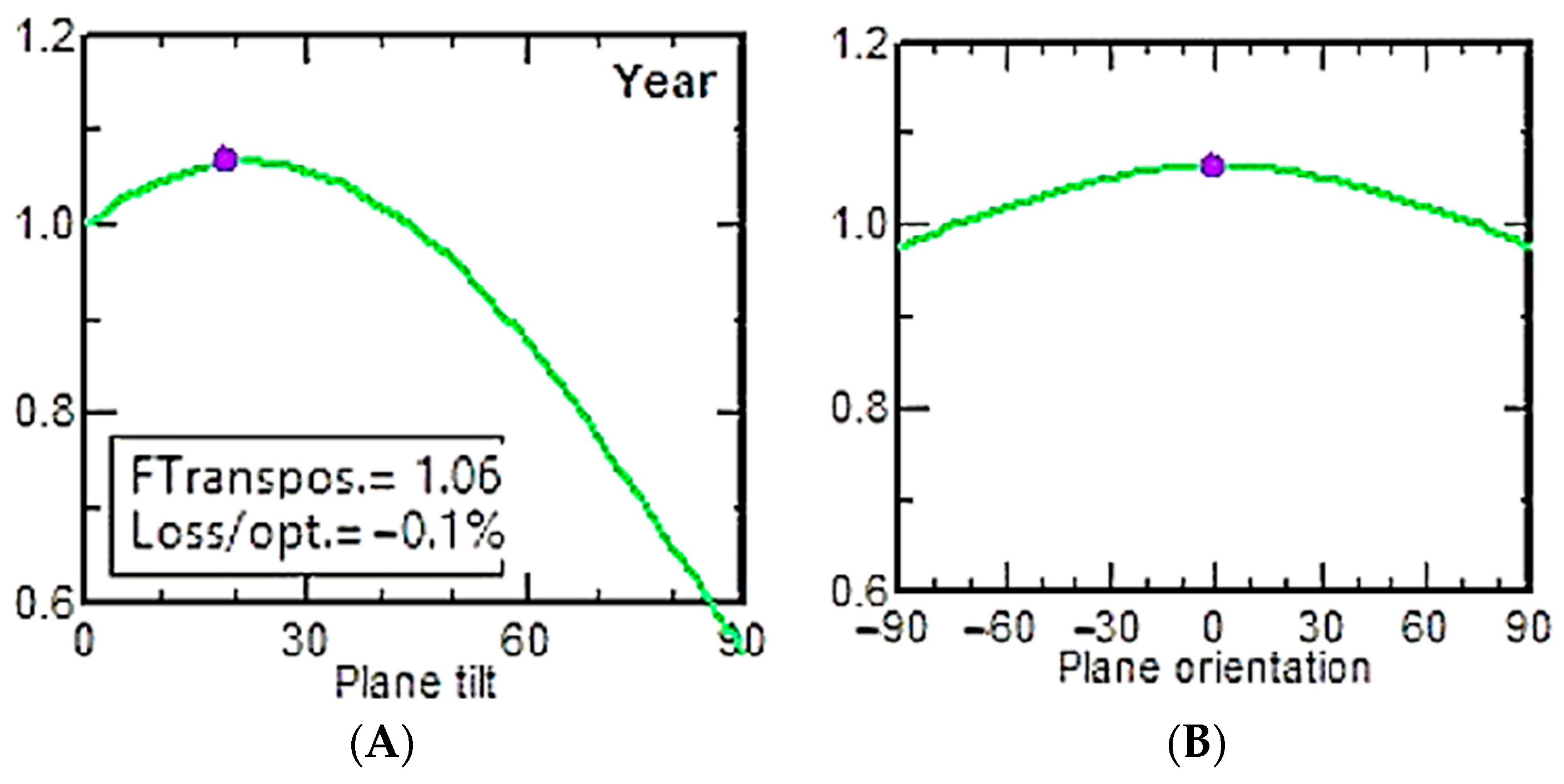
Similarly, the simulator registers the direction, angle, and inclination of the solar panels and predicts losses depending on the seasonal selection, as seen above. By selecting an annual average of 19°, it was verified that there are no losses. The simulator results are shown in Figure 12.

System performance was evaluated using two relative efficiency indicators. As illustrated in Figure 12A, a 19° tilt angle optimizes the configuration, achieving a solar radiation utilization rate of 106% (equivalent to a 1.06 ratio) relative to a horizontal surface. Furthermore, Figure 12B demonstrates that an azimuth orientation of 0° (true south) eliminates losses associated with angular deviation. Consequently, this specific configuration yields zero deviation losses (0.0%) relative to the theoretical optimum, thereby maximizing energy capture for the irrigation system.

3.2. Energy Balance and Losses

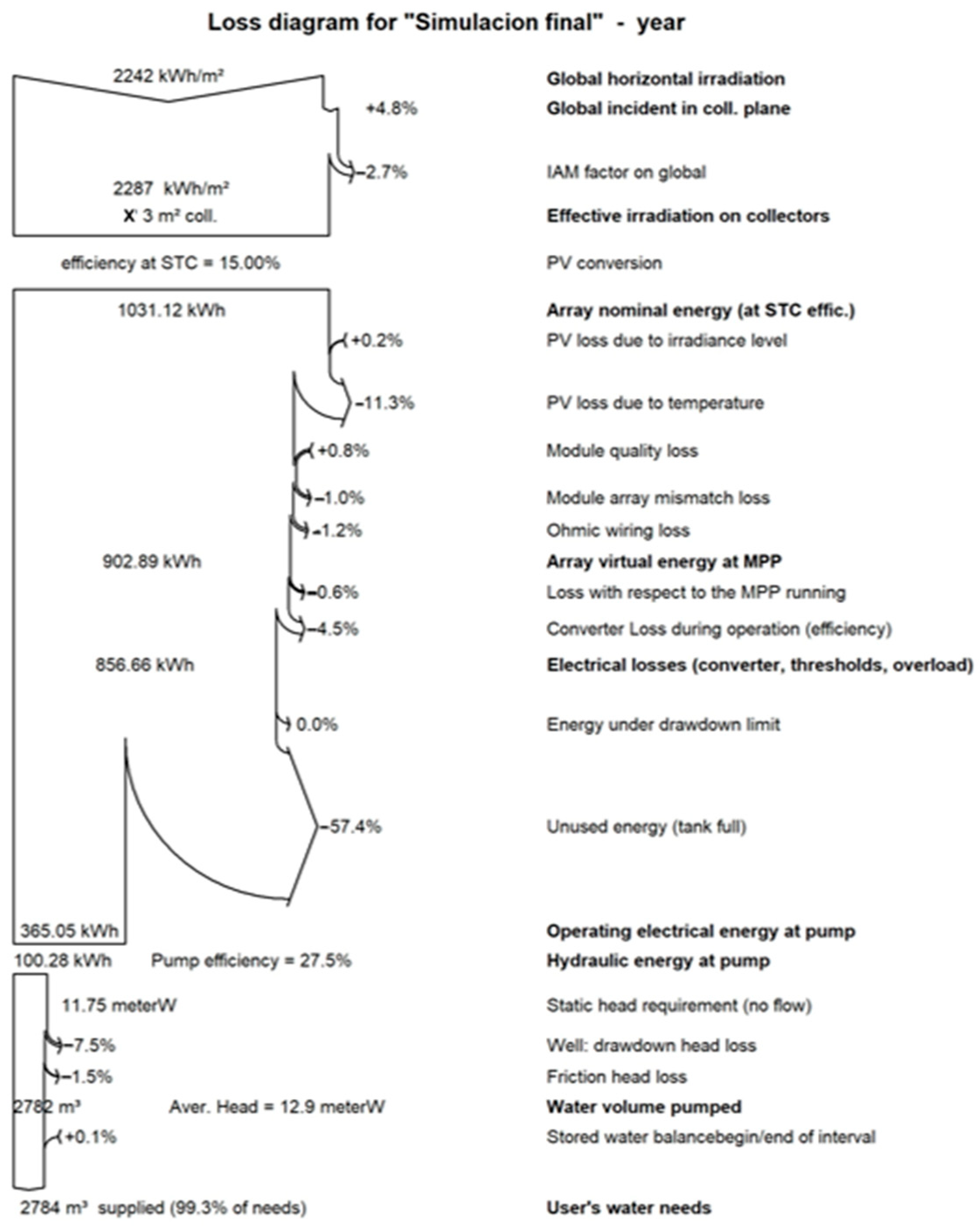
For the overall evolution of the proposed pumping system with the extension of the methodology, the loss diagram provided by the software was analyzed, allowing us to observe the main losses in the system, from solar generation, energy conversion and control, and energy conversion, excess energy (unused energy), and hydraulic and pumping losses, to see if it is capable of supplying the water demand of forage maize Figure 13 shows the loss diagram provided by the simulator.

This figure shows that the annual global horizontal irradiation reaches a value of 2242 kWh/m², which translates into an effective irradiation on the photovoltaic generator plane of 2287 kWh/m², considering corrections for orientation and angular incidence (IAM) of 2.7%. The modules achieve an efficiency of 15% under standard conditions (STC), which results in a nominal photovoltaic energy level of 1031.12 kWh/year.

Subsequently, the available energy is reduced due to temperature losses of 11.3%, photovoltaic module mismatch of 1%, and wiring losses (connection between panels) of 1.2%. After considering these losses, the effective energy available at the maximum power point (MPP) is reduced to 902.89 kWh, which would be the total solar generation.

In turn, there are additional electrical losses during the energy conversion stage when searching for the maximum power point (MPP) of 0.6%, together with electrical losses within the conversion of 4.5%, resulting in a useful energy of 856.66 kWh, of which the unused or surplus generated is 57.4% (491.6 kWh/year) due to the limitation of the storage tank, which shows an operational restriction and not a problem with the sizing of the photovoltaic generator.

The electrical energy used by the pump is 365.05 kWh per year, with a pump efficiency of 27.5% and a total system efficiency of 40.4%. The hydraulic system operates with an average total dynamic head of 12.9 mca, a value close to the theoretical requirement of 11.75 mca, confirming the appropriate selection and sizing of the pumping unit based on the methodological extension.

3.3. Monthly Operational Coverage

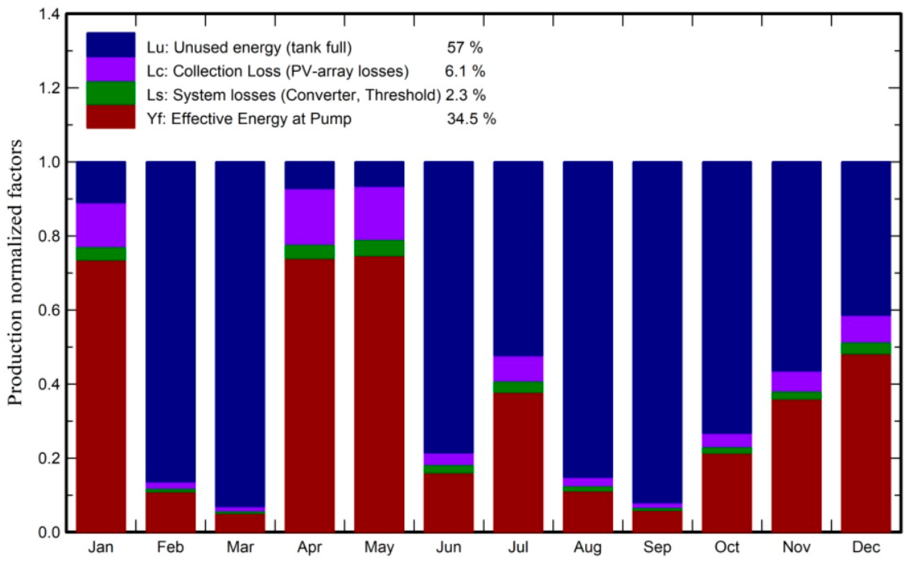
As a result, the volume pumped reaches 2782 m³ per year, which, considering our annual requirement of 2804 m₃, covers 99.3% of our water needs. These results show that the system performs consistently overall. This can be analyzed in greater detail in Figure 14.

This graph also shows that unused energy (Lu) accounts for 57% (491.6 kWh), total losses are 14.03% (3.1% from generation and 2.3% from system losses), giving usable energy for pumping of 34.5% (365.05 kWh/year). In the months with lower solar availability, a higher relative proportion of usable energy in the pump is observed, demonstrating that the system maintains operational stability and continuity in the water supply throughout the year. This performance is adequate with an annual pumped volume of 2782 m³ and 99.3% coverage of water demand, confirming that the design prioritizes hydraulic reliability over maximizing instantaneous energy use.

The monthly performance shows that, during the months with the highest irradiation, a considerable fraction of the available energy is not used due to the limitation imposed by hydraulic storage, which confirms that the system is not restricted by photovoltaic capacity but by the storage strategy adopted, which does not consider the chosen battery, since only the direct pumping part was simulated. For this reason, the potential for utilizing the energy surplus through electrical storage was evaluated. Based on the annual unused energy (Lu = 491.6 kWh/year) and a battery bank with 80% Depth of Discharge (DoD) providing a usable capacity (C_bat) of 1 920 Wh, the theoretical number of annual complete charges (C_C) is determined by Equation (16):

$${\mathit{C}}_{\mathit{C}}={\displaystyle \frac{L_u}{C_{bat}}}={\displaystyle \frac{\mathbf{491.6} \mathit{k}\mathit{W}\mathit{h}}{\mathbf{1.920} \mathit{k}\mathit{W}\mathit{h}}}=\mathbf{256} \mathit{c}\mathit{y}\mathit{c}\mathit{l}\mathit{e}\mathit{s}\mathbf{/}\mathit{y}\mathit{e}\mathit{a}\mathit{r}$$

(16)

The tank provides 75% operational coverage (273 days), indicating that the system operates predominantly under conditions of water self-sufficiency, with the deficit being limited to periods of low irradiation where the restriction is hydraulic rather than energy-related.

3.4. Tank Cover and Overflow

While Figure 14 showed the monthly behavior of excess energy and seasonal variability,

Table 13. Monthly system results.

Month	GlobEff kWh/m2	E_MPP kWh	E_Pump kWh	E_Exced kWh	Pressure mca	W_Pump m3/month	R_V m3/month	M_W m3/month
January	194.5	77.72	65.8	8.28	13.13	465.6	468.9	11.56
February	190.1	74.67	9.56	61.67	12.89	87.8	84.6	0
March	211.8	82.56	4.98	73.69	12.31	39.5	39.1	0
April	201.8	78.32	68.99	5.46	13.05	491.3	495.3	1.76
May	190	74.78	65.87	4.74	13.02	499.6	499.7	7.14
June	175	70	13.06	52.76	12.62	116.6	113.1	0
July	189.7	75.37	33.41	37.68	12.86	271.9	273.1	0
August	192.8	76.18	9.92	62.16	12.51	84.6	83.1	0
September	186.7	73.6	5.08	64.81	12.26	37.9	37.5	0
October	195.3	76.58	19.24	53.56	12.62	153	154.4	0
November	189.6	75.16	31.4	40.21	12.98	241.7	242.4	0
December	169.9	67.95	37.73	26.59	12.98	292.6	292.6	0
Year	2287.2	902.89	365.05	491.6	12.9	2782	2783.8	20.46

presents the monthly energy and hydraulic results of the photovoltaic pumping system. It summarizes the corrected global effective irradiation (GlobEff), the generator energy at the maximum power point (E_MPP), the electrical energy supplied to the pump (E_Pump), the unused energy associated with the full tank condition (E_Exced), as well as the volume of water pumped (W_Pump), the required volume (R_V), and the missing water (M_W).

When reevaluating the most critical months (January, April, and May), a significant change in the water deficit can be observed with respect to the initial analysis in Table 10. The initial sizing was based exclusively on water requirements, with April identified as the most critical month.

However, the simulation that integrates both the requirement and the effective pumping hours reveals that January has the highest monthly need, with a deficit of 11.56 m³/month (equivalent to 0.38 m³/day or 380 L per day), with a surplus energy of 8. 28 kWh considering the energy required from the battery to provide the additional pumping of 1 h and 10 min (17% of the battery’s useful capacity) and applying Equation (16), it is concluded that the battery can sustain this 17% discharge for 25 consecutive days. This value is significantly higher than the actual number of deficit events observed.

3.5. General Results

Finally, it is essential to emphasize the technical indicators that validate the design’s robustness.

Table 14. General results of the simulation.

Category	Concept	Value
Water	Annual pumped water	2782 m3
	Water requirements	2804 m3
	Water shortage (deficit)	0.80%
Energy	Pump energy	365 kWh
	Unused PV energy	492 kWh
Efficiencies	Unused fraction	54.40%
	System efficiency	40.40%

synthesizes the most relevant simulation data, confirming that the system not only satisfies the water demand but also operates within optimal safety margins and efficiency parameters. These results underscore the technical viability of the proposed solution for the study area.

The alignment between water demand and photovoltaic capacity, when integrated with the other system components, confirms that the proposed design offers greater operational robustness than the initial theoretical estimates. Although critical points of negative balance were identified in relation to physical storage levels, the inclusion of a backup electrical system and the management of excess energy ensure the continuity of supply.

These results demonstrate that the proposed methodological expansion facilitates a precise technical alignment between hydraulic requirements and solar generation.

Based on these results, the system was physically implemented in the case study to validate its performance under real operating conditions.

3.6. System Implementation and Validation

The photovoltaic pumping system was installed on 2 February 2026, in accordance with the sizing criteria established in the proposed methodology and its extension. During this phase, the pump was installed in the pre-prepared piping system at a depth of approximately 30 cm from the bottom of the well, in accordance with the manufacturer’s specifications.

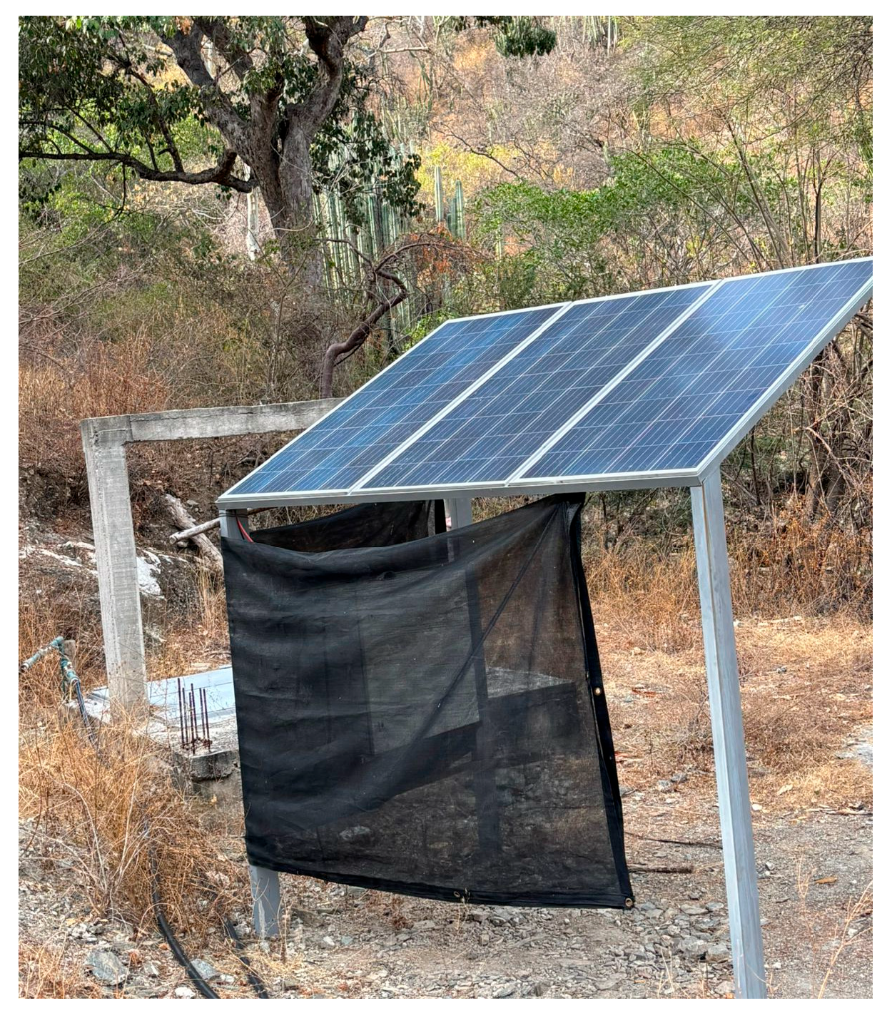
The photovoltaic system was mounted on a south-facing metal frame with a 19° tilt, where the solar modules were connected in parallel, as shown in Figure 15.

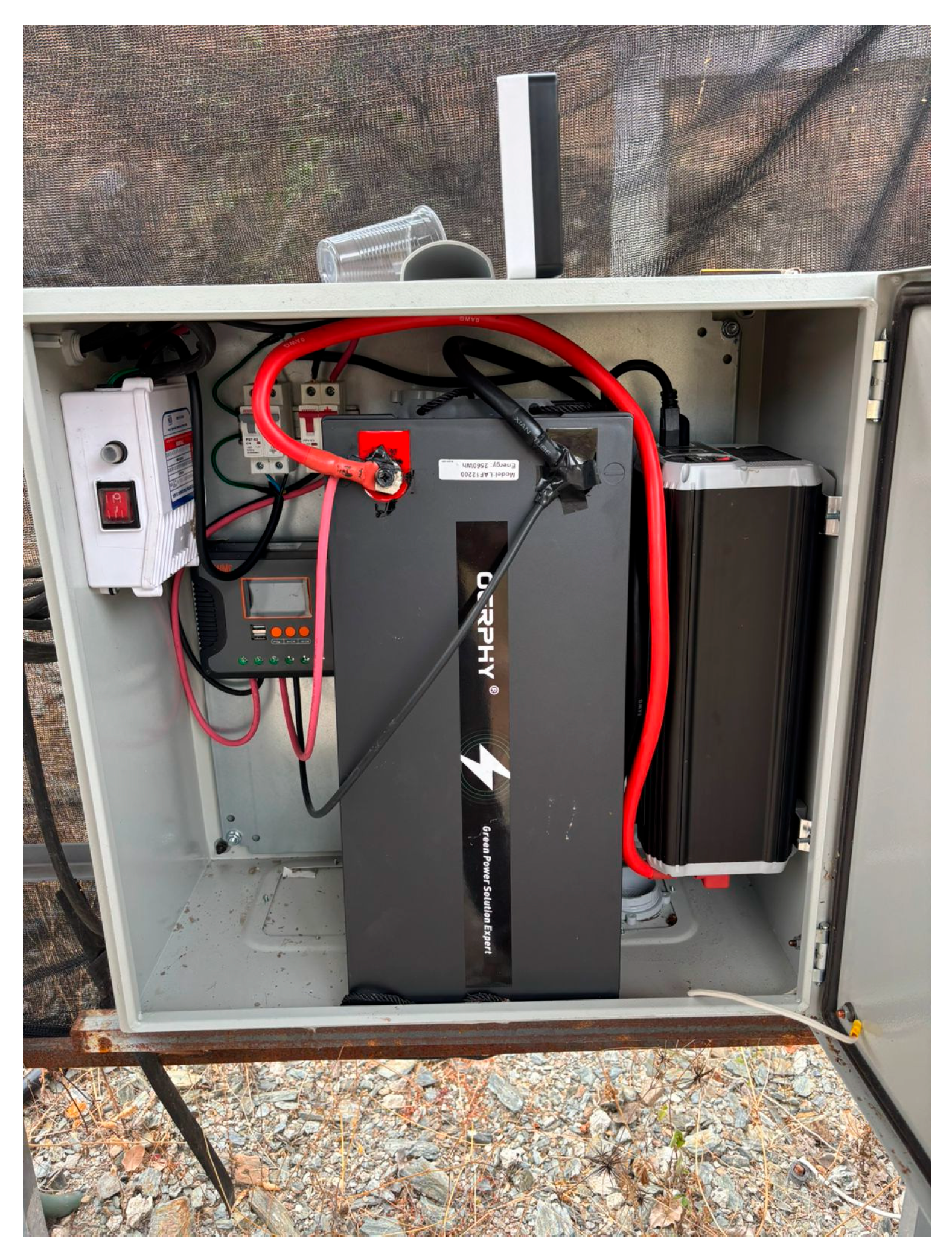
The wiring from the panels was routed to a metal enclosure, which housed the system’s main components: battery, inverter, controller, and pump start-up system. This configuration is designed to protect the equipment from adverse environmental conditions, such as humidity, dust, and direct sunlight, which can affect its service life. This phenomenon is illustrated in Figure 16.

The battery bank was interconnected using 4 AWG conductors, capable of managing continuous currents up to 100 A. This gauge ensures stability during pump startup peaks and consistent power delivery during non-peak solar hours. Similarly, the pump starter is linked to control relays via 10 AWG conductors, integrated with the solar controller to handle currents below 30 A, a standard configuration for small-scale photovoltaic systems.

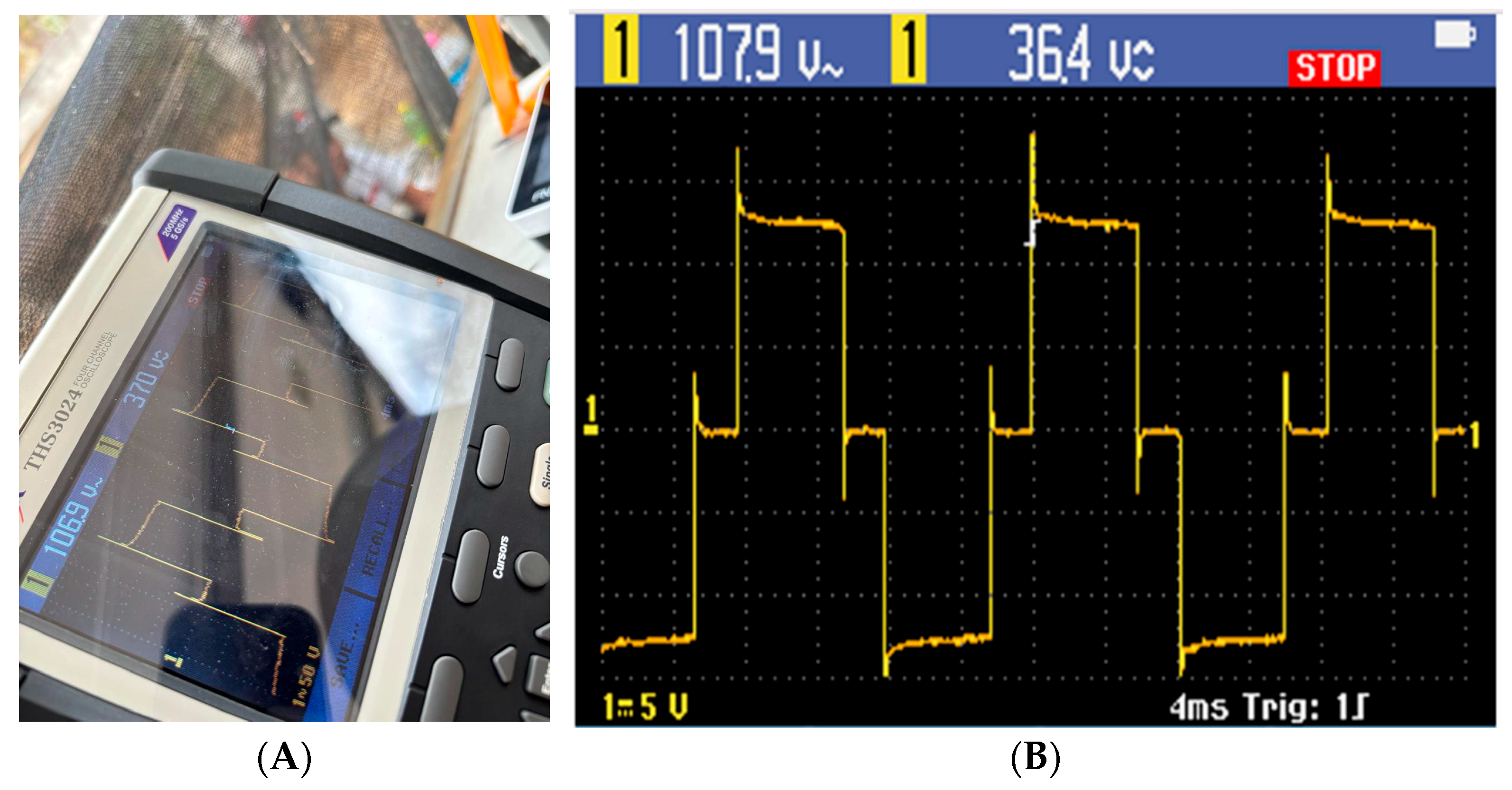
To validate system performance, field data were collected between 14:50 and 16:00. A Tektronix THS3024 oscilloscope was used to monitor critical variables and ensure high-accuracy signal sampling.

As shown in Figure 17, the pump voltage at 15:00 exhibits a stepped waveform, characteristic of the modified sine wave inverter used in this study. This output aligns with the technical specifications of the designated inverter model and confirms its correct integration into the autonomous pumping circuit.

The observed value of 107.9 V corresponds to the effective RMS voltage delivered to the pump, which is close to the pump’s nominal operating voltage (110 V), confirming the delivered supply. Meanwhile, the value of 36.4 V for this indicator is the result of integrating the non-sinusoidal waveform at a specific sampling point. Since this is a stepped waveform, the difference between the RMS value and the average is expected behavior due to the signal’s waveform shape. Similarly, the 1–5 V indicator corresponds to a vertical scale on the oscilloscope (5 V per division), used solely to visualize the signal, without directly representing the system’s actual voltage.

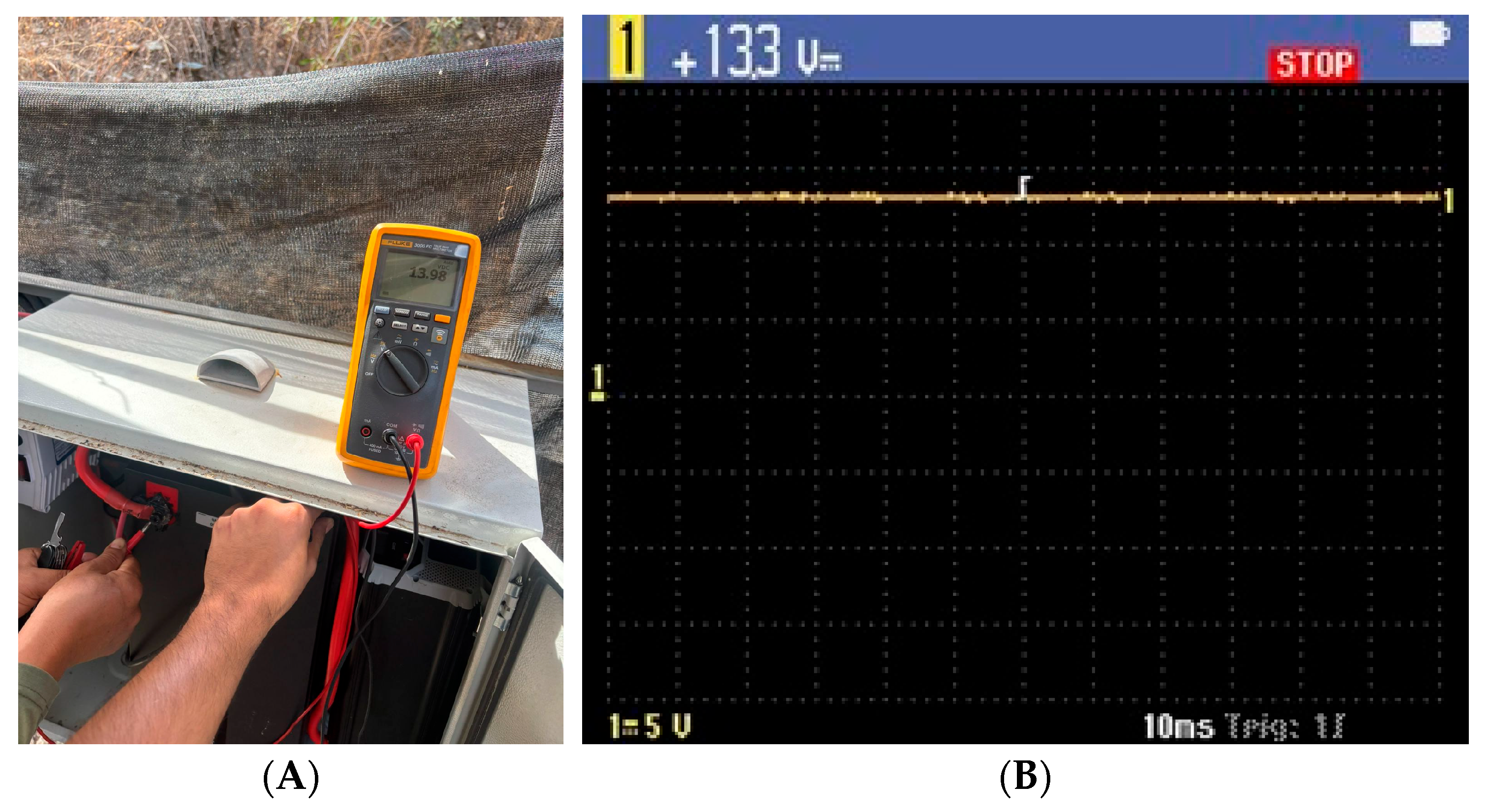
To complement the previous tests, the battery voltage was measured to verify its operation. The measurements taken from 3:15 to 3:00 PM in Image A show the monitoring with a multimeter, and these were also recorded with the oscilloscope; they can be seen in Figure 18.

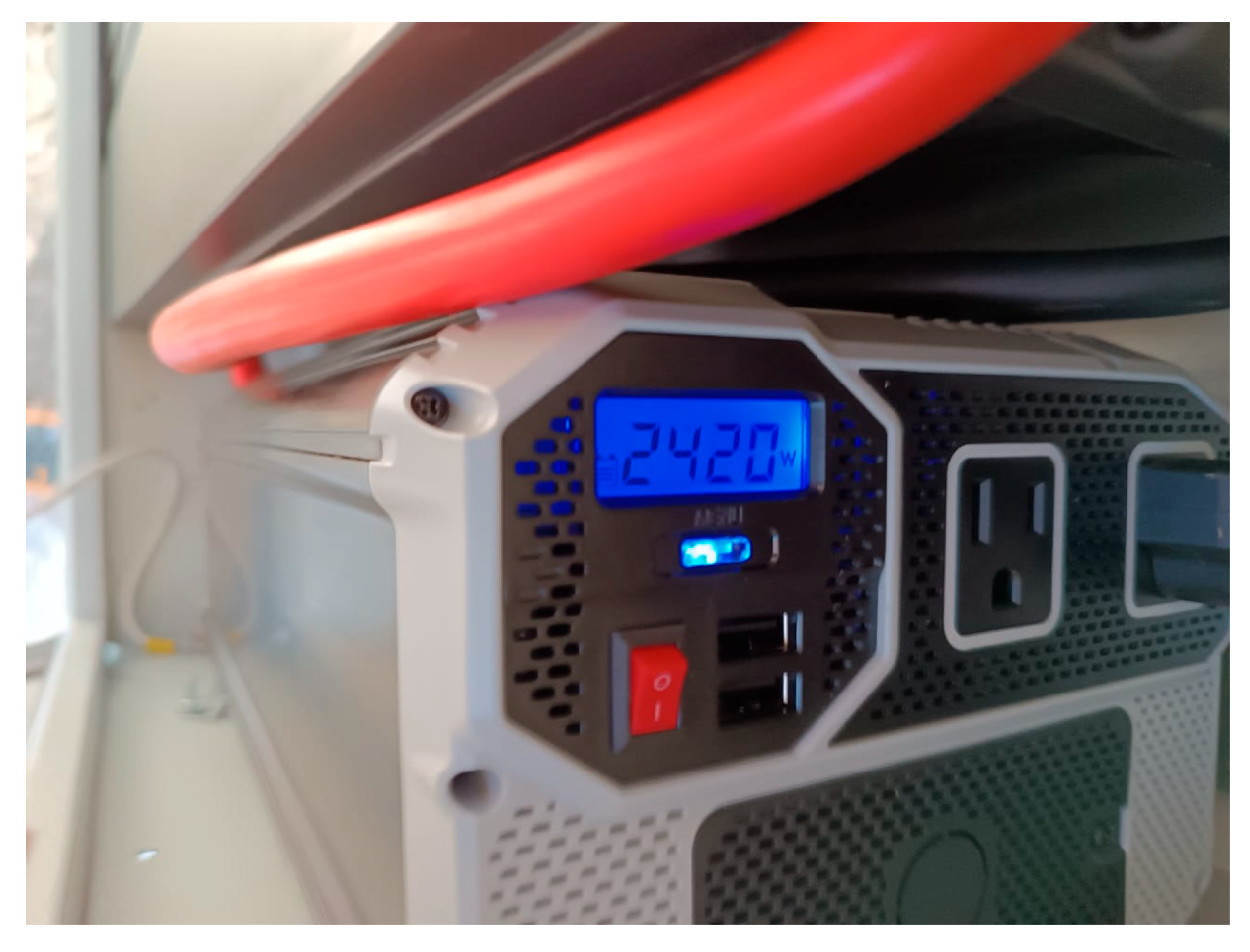
The voltage level recorded in both cases is close to 13 V, which confirms that the battery is at an optimal charge; furthermore, the oscilloscope monitoring shows stable behavior without any variation that could compromise the inverter’s interaction with the battery. Furthermore, the power delivered by the inverter during the tests, recorded at 3:50 p.m., is shown below in Figure 19.

An operating power of 2420 W was observed, confirming the pumping system’s performance under real field conditions. The close relationship between this experimental value and the theoretical demand of 2247 W confirms the validity of the calculation method used for system sizing.

The difference between the two is attributed to variations inherent in real operating conditions; however, this deviation remains within an acceptable range, guaranteeing a sufficient energy supply to ensure operational continuity.

4. Discussion and Conclusions

The combination of the general methodology and its proposed application demonstrates that it is possible to develop a pumping system that is both technically and economically sound, even in rural settings where conventional alternatives are not feasible.

The initial investment in the photovoltaic system guarantees economic benefits associated with the production of one hectare of forage maize, the commercialization of which allows for an investment recovery period of approximately two years. This result is supported by an LCOE of 14.03 MXN/kWh. While this value is higher than the grid-connected agricultural pumping tariff (≈0.74 MXN/kWh), such a comparison overlooks the context of isolated areas where extending the electrical grid is required. When accounting for this additional infrastructure, the equivalent LCOE in this case study increases to 39.09 MXN/kWh. This implies that the proposed photovoltaic system is the economically superior alternative to grid extension.

In comparison, diesel-based pumping systems, which present a lower initial investment but high operating costs, fuel price volatility, and high CO₂ emissions, limit their long-term sustainability. In contrast, the photovoltaic system is not only cleaner but also more stable and economically favorable for agricultural applications in regions such as the Mixteca Poblana. Consequently, the proposed photovoltaic system stands as the most economically viable and competitive alternative in rural scenarios lacking electrical coverage.

From a technical standpoint, simulations under realistic conditions—considering the system’s loss diagram and the analysis of useful energy for pumping—verified a 99.08% coverage of the water demand. The integration of a battery system ensures irrigation continuity and stable operation, even during startup conditions with current peaks. The overall efficiency obtained (40.4%) is higher than that reported in direct pumping systems with MPPT (30.92%) [4] and falls within the range of efficiencies measured in real-world conditions, which oscillate between 27.82% and 70.64% [36]. These figures confirm that the design operates within appropriate performance ranges.

It is important to highlight that the pump used showed an efficiency of 27.5%, a value attributed to its operation under real-world photovoltaic supply conditions, where irradiance variability directly influences performance. Nevertheless, the system as a whole compensates for this limitation through the proper integration of components. This suggests that, in solar systems, the individual efficiency of each element is less decisive than the global synergy of the design, as the latter defines the system’s capacity to reliably meet demand.

Since the system proved to be technically and economically viable, it was implemented in the case study. Field tests demonstrate that it operates within the predicted parameters, validating the methodology. More importantly, it provides the case study with water security and food security, contributing to the sustainable development of the Mixteca Poblana driven by renewable energy.

In summary, these findings show that the use of a structured methodological framework for the proper selection of components allows for the development of replicable solutions in rural contexts, minimizing investment risk and maximizing social and productive benefits.

As future work, it is relevant not only to monitor the system under prolonged real-world conditions but also to evaluate it in dynamic economic scenarios, considering variations in component costs and agricultural market conditions. This will consolidate the proposal as a robust and scalable tool for rural development based on renewable energies.

References

1. Our World in Data. Access to Energy. Available online: https://ourworldindata.org/energy-access (accessed on 16 April 2025).
2. Ahmed, F.; Al-Abri, R.; Yousef, H.; Massoud, A.M. An optimal energy dispatch management system for hybrid power plants: PV grid battery diesel generator pumped hydro storage. IEEE Access 2024, 12, 143307–143326. [Google Scholar] [CrossRef]
3. Badamshina, S.; Klokov, A.; Loktionov, E. Opportunities for economic efficiency increase in renewable energy powered off-grid systems. In Proceedings of the 2023 International Ural Conference on Electrical Power Engineering, Magnitogorsk, Russia, 29 September–1 October 2023; pp. 583–588. [Google Scholar] [CrossRef]
4. Orts-Grau, S.; Gonzalez-Altozano, P.; Gimeno-Sales, F.J.; Balbastre-Peralta, I.; Marquez, C.I.M.; Gasque, M.; Segui-Chilet, S. Photovoltaic water pumping: Comparison between direct and lithium battery solutions. IEEE Access 2021, 9, 101147–101163. [Google Scholar] [CrossRef]
5. Diop, L. Technical and economic feasibility of solar irrigation pumping systems: A review. Knowl.-Based Eng. Sci. 2020, 1, 1–22. [Google Scholar] [CrossRef]
6. Lilhare, A.S.; Kadwane, S.G. Maximizing solar water pump efficiency: Exploring MPPT strategies for optimization. AIP Adv. 2024, 14, 045131. [Google Scholar] [CrossRef]
7. Mazloumi, A.; Poolad, A.; Mokhtari, M.; Babaee Altman, M.; Abdelaziz, A.; Elsisi, M. Optimal sizing of a photovoltaic pumping system integrated with a water storage tank considering cost/reliability assessment. Mathematics 2023, 11, 463. [Google Scholar] [CrossRef]
8. Xu, Z.; Chen, X. Optimization of the coupling between water and energy consumption in a smart integrated photovoltaic pumping station system. Water 2024, 16, 1493. [Google Scholar] [CrossRef]
9. Gimeno-Sales, F.J.; Orts-Grau, S.; Escribá-Aparisi, A.; González-Altozano, P.; Balbastre-Peralta, I.; Martínez-Márquez, C.I.; Gasque, M.; Seguí-Chilet, S. PV monitoring system for a water pumping scheme with a lithium-ion battery using open-source software and IoT technologies. Sustainability 2020, 12, 10651. [Google Scholar] [CrossRef]
10. Parveen, H.; Sharma, U.; Singh, B. Solar water pumping system with captive energy storage functionality. In Proceedings of the IEEE Energy Conversion Congress and Exposition (ECCE), Vancouver, BC, Canada, 10–14 October 2021; pp. 186–191. [Google Scholar] [CrossRef]
11. Mruma, I.S.; Ayeng’o, S.P. Designing a model of solar photovoltaic water pumping system for off-grid localities in Tanzania. Tanzan. J. Eng. Technol. 2023, 42, 154–170. [Google Scholar] [CrossRef]
12. Almaidan, M.; Tenruh, M.; Gabrovska-Evstatieva, K.; Valov, N.; Keseev, V.; Kadirova, S.; Mihailov, N. Performance analysis of a 5 kW photovoltaic installation for water pumping in rural areas in Yemen. In Proceedings of the 9th International Conference on Energy Efficiency and Agricultural Engineering, Ruse, Bulgaria, 27–29 June 2024; pp. 1–4. [Google Scholar] [CrossRef]
13. Aliyi, M.; Nuru, N. Simulation of photovoltaic water pumping systems for small-scale irrigation and rural electrification using PVsyst. Int. J. Energy Power Eng. 2020, 9, 49–56. [Google Scholar] [CrossRef]
14. Khan, M.S.; Tahir, A.; Alam, I.; Razzaq, S.; Usman, M.; Tareen, W.U.K.; Baig, N.A.; Atif, S.; Riaz, M. Assessment of solar photovoltaic water pumping of WASA tube wells for irrigation in Quetta Valley aquifer. Energies 2021, 14, 6676. [Google Scholar] [CrossRef]
15. Moussa, A.R.S.; Ali, A.; Boukar, M.; Madougou, S. Study of a photovoltaic solar pumping system for irrigation: Case of the Adaraoua site. Adv. Image Video Process. 2022, 10, 121–131. [Google Scholar] [CrossRef]
16. Sarwar, A.; Iqbal, M.T. Design and optimization of solar PV system for a fish farm in Pakistan. In Proceedings of the 2022 IEEE 12th Annual Computing and Communication Workshop and Conference (CCWC), Las Vegas, NV, USA, 26–29 January 2022. [Google Scholar] [CrossRef]
17. Contigo, C. Contratación para Clientes de Tarifa Doméstica; Comisión Federal de Electricidad: Mexico City, Mexico, 2022. [Google Scholar]
18. Comisión Federal de Electricidad (CFE). Catálogo de Precios. Available online: https://app.cfe.mx/aplicaciones/otros/aportaciones/ (accessed on 14 April 2025).
19. Lorenzo, C.; Almeida, R.H.; Martínez-Núñez, M.; Narvarte, L.; Carrasco, L.M. Economic assessment of large power photovoltaic irrigation systems in the ECOWAS region. Energy 2018, 155, 992–1003. [Google Scholar] [CrossRef]
20. Catuogno, G.; Mickelson, A.; Chalbaud, J.; Frías, G.; Catuogno, C.; Aleman, M. Water and solar energy for humanitarian aid in rural communities. In Proceedings of the 2023 IEEE Global Humanitarian Technology Conference (GHTC), Radnor, PA, USA, 12–15 October 2023; pp. 66–69. [Google Scholar] [CrossRef]
21. Ibrahim, S.M.A.; El-Ghetany, H.H.; Shabak, A.G.M. Comprehensive design tool for sizing solar water pumping systems in Egypt. Appl. Sol. Energy 2020, 56, 18–29. [Google Scholar] [CrossRef]
22. Gasque, M.; Gonzalez-Altozano, P.; Gimeno-Sales, F.J.; Orts-Grau, S.; Balbastre-Peralta, I.; Martinez-Navarro, G.; Segui-Chilet, S. Energy efficiency optimization in battery-based photovoltaic pumping schemes. IEEE Access 2022, 10, 54064–54078. [Google Scholar] [CrossRef]
23. NASA POWER. POWER Data Access Viewer. Available online: https://power.larc.nasa.gov/data-access-viewer/ (accessed on 14 April 2025).
24. Guevara, M.; Manzini, F.; Sánchez-Juárez, A. Technical and economic analysis for photovoltaic systems in agricultural zones of Mexico City. Energy Sustain. Dev. 2025, 87, 101743. [Google Scholar] [CrossRef]
25. Mehleri, E.D.; Zervas, P.L.; Sarimveis, H.; Palyvos, J.A.; Markatos, N.C. Determination of optimal tilt angle and orientation for PV arrays. Renew. Energy 2010, 35, 2468–2475. [Google Scholar] [CrossRef]
26. Chen, H.; Wang, Y.; Yang, H.; Shi, Y.; Yu, B.; Yang, J. Experimental and simulation study on bifacial photovoltaic modules integration with buildings. Therm. Sci. 2022, 26, 4413–4422. [Google Scholar] [CrossRef]
27. Rengma, N.S.; Yadav, M.; Kishor, N. Solar photovoltaic water pumping system: Optimal configuration investigation. Renew. Energy Focus 2023, 46, 236–255. [Google Scholar] [CrossRef]
28. INEGI. Resultados Definitivos del Censo Agropecuario en el Estado de Puebla; INEGI: Mexico City, Mexico, 2023. [Google Scholar]
29. Secretaría de Agricultura y Desarrollo Rural. Se Incrementa Producción de Maíz con Alternativas de Labranza en la Mixteca Poblana. Available online: https://www.gob.mx/agricultura/prensa/se-incrementa-produccion-de-maiz-con-alternativas-de-labranza-en-la-mixteca-poblana (accessed on 14 April 2025).
30. Allen, R.; Pereira, L.; Raes, D.; Smith, M. FAO Irrigation and Drainage; Paper No. 56; FAO: Rome, Italy, 1998. [Google Scholar]
31. Wielgat, R.; Ko£Odziej, A.; Candela, L.; Lisowska-Lis, A.; Jasielski, J.; Chlastawa, Ł.; Touhami, M.; Jaramillo, M.F. A concept of smart agro-photovoltaic tunnels. IEEE Access 2024, 12, 40765–40794. [Google Scholar] [CrossRef]
32. Bojnec, Š.; Daraz, U.; Khan, Y. Harvesting sunlight: Agro-photovoltaic systems for sustainable agriculture. Energies 2024, 17, 3310. [Google Scholar] [CrossRef]
33. Guerra, P.J.; Lara, C.R.; Saucedo, R.A. Paquete Tecnológico para la Producción de Maíz Forrajero en Chihuahua; INIFAP: Mexico City, Mexico, 2014. [Google Scholar]
34. Iqbal, M.T. A comparative study of solar water pump storage systems. In Proceedings of the 2022 IEEE 12th Annual Computing and Communication Workshop and Conference CCWC, Las Vegas, NV, USA, 26–29 January 2022. [Google Scholar] [CrossRef]
35. Oladigbolu, J.O.; Ramli, M.A.M.; Al-Turki, Y.A. Feasibility study of hybrid renewable systems for rural electrification. IEEE Access 2020, 8, 171643–171663. [Google Scholar] [CrossRef]
36. Meyer, J.; von Solms, S. Solar powered water security for rural development. IEEE Access 2018, 6, 20694–20703. [Google Scholar] [CrossRef]
37. Rezk, H.; Rezk, H.; Al-Dhaifallah, M.; Hassan, Y.B.; Ziedan, H.A. Optimization of hybrid PV–diesel–battery systems. IEEE Access 2020, 8, 102512–102529. [Google Scholar] [CrossRef]
38. Habyarimana, M.; Dorrell, D.G.; Musumpuka, R. Reduction of starting current in induction motors. Energies 2022, 15, 3848. [Google Scholar] [CrossRef]
39. Rumbayan, M.; Pundoko, I.; Sompie, S.R.; Ruindungan, D.G. Integration of smart water management and PV pumping systems. Results Eng. 2025, 25, 103966. [Google Scholar] [CrossRef]
40. Klokov, A.V.; Tutunin, A.S.; Sharaborova, E.S.; Korshunov, A.A.; Loktionov, E.Y. Inverter heat pumps as variable load for off-grid systems. Energies 2023, 16, 5987. [Google Scholar] [CrossRef]
41. Montesillo-Cedillo, J.L. Rendimiento por hectárea del maíz grano en México: Distritos de riego vs. temporal. Econ. Inf. 2016, 398, 60–74. [Google Scholar] [CrossRef]
42. Unisem. Análisis de Costos de Producción de Maíz en 2025. Available online: https://semillastodoterreno.com/2025/04/analisis-de-costos-de-produccion-de-maiz-en-2025/ (accessed on 28 August 2025).
Figure 1. Diagram of the general methodology for sizing photovoltaic pumping systems, illustrated in the applications of [9,10].
Sci 08 00126 g001
Figure 2. Proposed methodology for component selection.
Sci 08 00126 g002
Figure 3. Hourly distribution of solar radiation in the case study [23].
Sci 08 00126 g003
Figure 4. Dimensions of the well in the case study.
Sci 08 00126 g004
Figure 5. Average historical ambient temperature of the case study for the year 2022.
Sci 08 00126 g005
Figure 6. Relative humidity for the case study site.
Sci 08 00126 g006
Figure 7. Wind speed for the case study site.
Sci 08 00126 g007
Figure 8. Monthly average solar insolation of the case study.
Sci 08 00126 g008
Figure 9. Historical precipitation data for the case study site.
Sci 08 00126 g009
Figure 10. Total water demand of the agricultural system.
Sci 08 00126 g010
Figure 11. Current peak during start-up of the 1 hp Hyundai pump.
Sci 08 00126 g011
Figure 12. Solar optimization analysis: (A) Variation in efficiency due to plane inclination and (B) Variation due to orientation (azimuth). The green line represents the system performance for different tilt and orientation angles, while the purple point indicates the selected configuration of 19° tilt and 0° azimuth, corresponding to the optimal annual solar energy capture.
Sci 08 00126 g012
Figure 13. Diagram of energy losses in the photovoltaic pumping system obtained through simulation in PVsyst 8.0. The symbol “×” was used to represent the multiplication between the incident irradiation and the collector area of the photovoltaic array.
Sci 08 00126 g013
Figure 14. Standard monthly production and loss factors for the photovoltaic pumping system.
Sci 08 00126 g014
Figure 15. Panels installed in the case study.
Sci 08 00126 g015
Figure 16. Components stored in the safe.
Sci 08 00126 g016
Figure 17. Pump voltage analysis: (A) Physical measurement in the field; (B) Signal capture with an oscilloscope.
Sci 08 00126 g017
Figure 18. Battery bank monitoring: (A) Terminal voltage measurement; (B) Signal stability on the oscilloscope.
Sci 08 00126 g018
Figure 19. Power Inverter.
Sci 08 00126 g019