The Garisenda Tower in Bologna: Damage Assessment Results from Principal Component Analysis, Acoustic Emission, and Nonlinear Finite Element Analyses Involving Creep and Smeared Cracking

Abstract

The Garisenda Tower, along with the neighboring Asinelli Tower, is arguably the symbol of the city of Bologna. They are the sole remnants of about one hundred towers that formed the city’s skyline in medieval times. As such, the monitoring of their state of health has been of great interest to the scientific community for more than a century—one example being the studies of Prof. Cavani in the early 1900s. The Garisenda Tower, famous for its impressive lean, is the object of Structural Health Monitoring (SHM) involving a multitude of devices. Some examples are a 30 m long pendulum installed on the inside of the tower to measure the planar displacement of the tower’s top; Fiber-Optical Strings (FOSs) installed in the walls of the basement to measure their vertical deformation; and piezoelectric acoustic emission (AE) sensors, also installed on the walls of the tower’s basement to detect elastic waves generated by micro-cracking. This rich experimental setup allows for the investigation of the tower’s stability and damage assessment. In this work, attention is focused on two analyses: The first is a Principal Component Analysis (PCA) study that investigates the correlation between AE data and other SHM data, such as in situ temperature, pendulum displacement, and AE rate. The second analysis corresponds with numerical finite element (FE) studies that assess damage in the base of the tower. Initially, the Smeared Cracking material model is used to understand which zones of the tower are more damaged. Moreover, a possible critical scenario due to increasing tower tilt is investigated. Finally, a viscoelastic formulation of the materials at the base of the tower is used to account for creep to understand the possible viscous effects at the base of the tower.

1. Introduction

The Garisenda Tower and the neighboring Asinelli Tower are the last surviving examples of approximately one hundred towers that once dominated Bologna’s medieval cityscape. Erected in the twelfth century alongside the Asinelli Tower, the structure was commissioned by the Garisendi family, hence its name. In 1351, however, the tower’s structural stability was compromised by foundation failure, which induced a marked inclination. To mitigate safety hazards, its original height was subsequently diminished by thirteen meters, from 61 to 48 m.

These towers represent two of Bologna’s most iconic landmarks and, as such, interest in their Structural Health Monitoring has attracted scientific attention for over a century—exemplified by Prof. Cavani’s pioneering investigations as early as 1910 [1], where he recorded a series of daily displacement measurements of the top, obtained from a mechanical pendulum, to study its evolution through the years.

The influence of material degradation, together with the integration of in situ monitoring data and numerical methods (such as FEA simulations), has been examined in [2,3], where material degradation and aging have been identified as among the potential contributors to the progressive increase in the inclination of the Garisenda. The FOS strain monitoring analysed in [4] revealed long-term settlement trends as well as strain responses induced by dynamic events such as seismic activity. Environmental, seismic, and anthropogenic effects were also investigated in [5,6]. Long-term structural change in the Garisenda, in particular from the last decade, has been studied in [7]. To this extent, the authors of the current work have also conducted studies focusing on numerical modelling for masonry structures monitored by AE [8], and recently focused on thermal effects [9,10,11,12]. Figure 1 depicts a xylography from the early 1900s of the two towers, and a picture of them and Piazza Maggiore before their closing to visitors.

The Garisenda is currently equipped with an extensive Structural Health Monitoring (SHM) system comprising multiple sensor types. Acoustic emission (AE) sensors are installed in the base walls, designed to register elastic waves produced by material micro-cracking. A 30 m electromechanical pendulum, installed on the inside, tracks in-plane displacements of the top of the tower. Fiber-Optic Strings (FOSs) are installed in the base walls to measure strains. Lastly, four external wire extensometers, thermometers, and inclinometers installed in the base complete the rich in situ setup. Together these systems work in synergy to give real-time insight into the structural health of the Garisenda.

This work concentrates on three main analyses: the first, Principal Component Analysis (PCA), examines the correlation between data from the SHM system, including ambient temperature near the tower, pendulum displacements, and AE measurements. The second analysis involved nonlinear finite element models to characterize the inelastic (irreversible) damage in the tower. The computational study employs a Smeared Cracking approach, identifying critical damage zones within the tower under augmented inclination, which could represent soil and/or foundation deterioration. Subsequently, the investigation incorporates a viscoelastic constitutive model instead, to represent time-dependent creep behavior. The model is calibrated using the in situ pendulum displacements, which as far as the authors know represents a novel approach. The model is viewed as a base for comparison for future studies which could aim to enrich the material behavior with damage and other phenomena, for example, (visco)plasticity.

1.1. Acoustic Emission

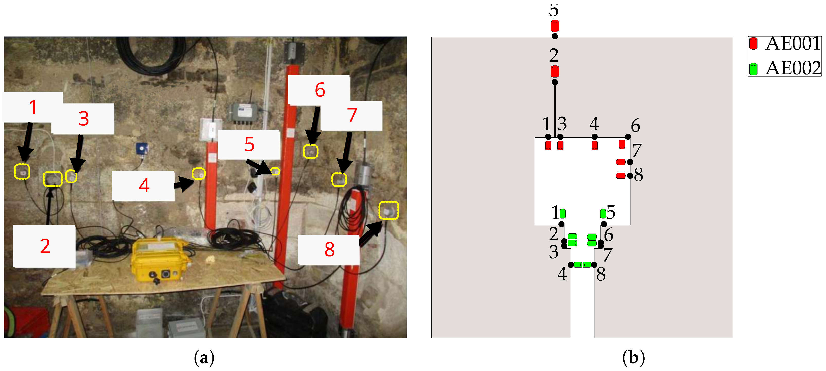
A custom-designed monitoring system capable of detecting acoustic emissions (AEs) was installed at the base of the Garisenda Tower. The system is comprised of two devices, AE001 and AE002, each featuring eight channels connected to piezoelectric sensors. The system was installed in order to investigate micro-cracking and thus to allow for structural assessment of the base of the tower. The first device, AE001, was put in place on 31 May 2019. Its sensors are installed in the eastern (leaning) side of the tower, with sensor CH2 being located inside the base casing, and CH5 being close to the outside wall (it was previously also located in the inner wall but was relocated). The second device, AE002, was added on 14 March 2023. Its sensors are located on the western side of the tower, close to the entrance. The sensors (Lunitek AEmission LT18-003-PRD00-R0) have a frequency range of 15–625 kHz. They are securely fastened to the tower’s inner wall using high-strength adhesive. Based on the ongoing AE field monitoring on the Garisenda Tower, only AE signals within a frequency range of 50–400 kHz, with an amplitude ≥ 0.7 mV, and a number of oscillations (ring-down count) ≥ 3 were considered, with signals that did not fall into these specifications discarded as noise. Figure 2 shows the installation of the piezoelectric sensors at the tower’s base, as well as a schematic diagram of their arrangement, providing a visual representation of the setup.

1.2. Pendulum

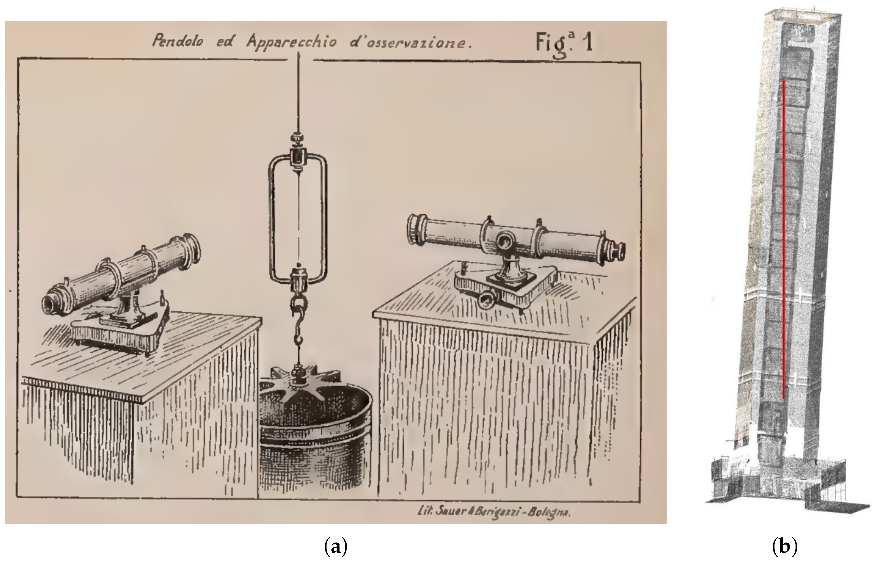
In February 2021, a 30 m pendulum was installed inside the tower by the company RTeknos s.r.l (https://www.rteknos.it/, accessed 27 October 2025) to measure the planar movement of its top in comparison with the base. This modern monitoring system finds inspiration in a mechanical pendulum installed inside the Garisenda as early as the beginning of the 20th century by Prof. Cavani with the same scope (Figure 3). The pendulum consists of a steel wire attached to a 15 kg mass submerged in a viscous fluid, which serves to provide damping. The position of the wire is monitored by a telecoordinometer, comprising a unit equipped with photocells arranged in transmitter–receiver pairs, actuated by an electric motor and supplied with power through a cable fitted with connectors. It can detect displacements of up to 100 mm in the south-east direction (X-axis) and up to 50 mm in the north-east direction (Y-axis). The pendulum’s margin of error is 0.075% of the maximum reading. This translates to an error range of 0.075 mm in the X direction and 0.0375 mm in the Y direction. The system also records the internal temperature at the base of the tower.

1.3. Fiber-Optical Strings

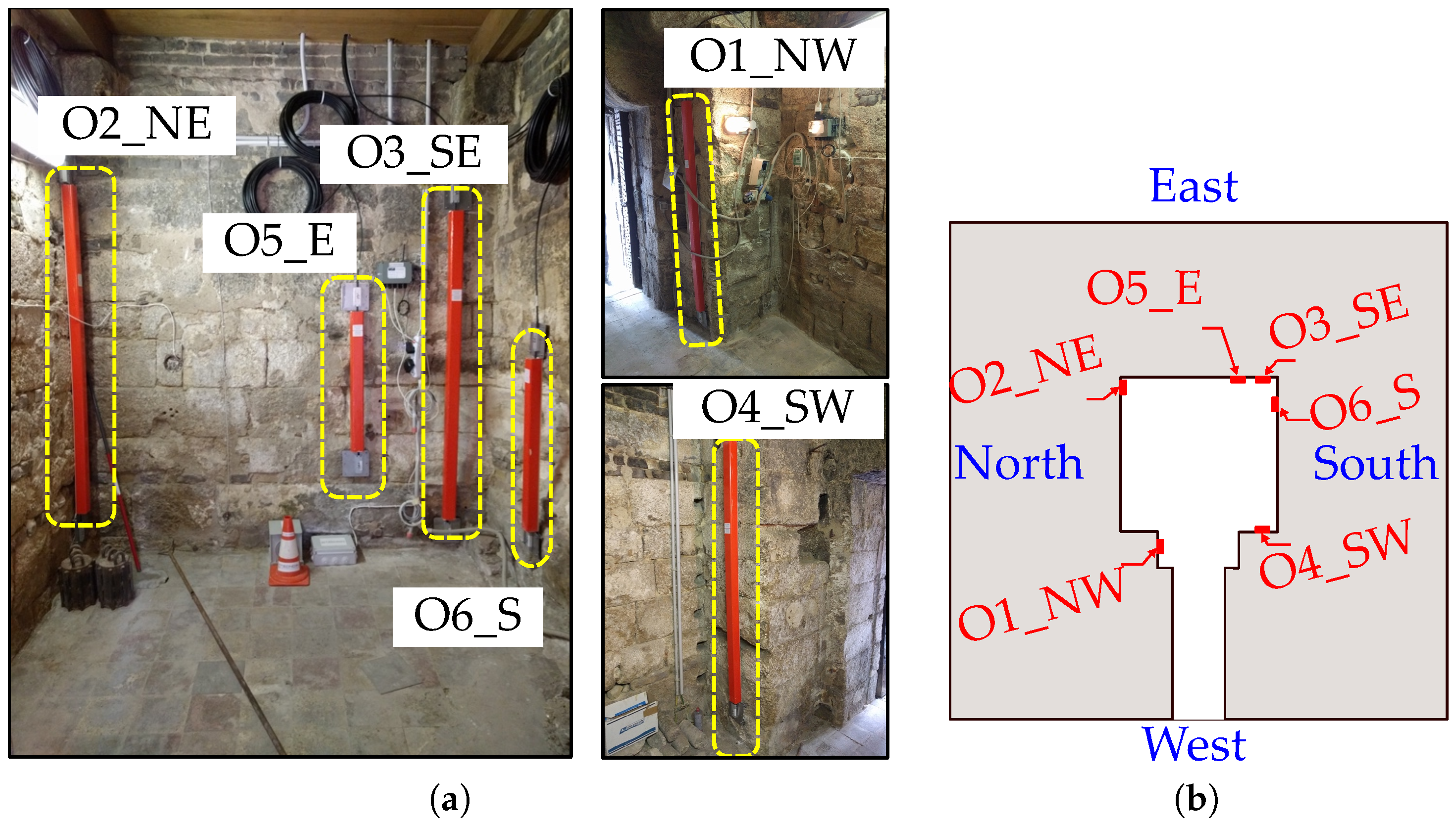
Eight FOS sensors were placed vertically on the inner walls of the base of the tower by OSMOS Group (https://www.osmos-group.com/en, accessed 27 October 2025). Six of them are shown in Figure 4; the other two were installed at the end of 2023 but were not considered for the present analysis. The FOSs were installed to measure strains in the base—the four 2 m long strings were installed to measure global strains in the base, while the two 1 m long strings were installed to measure local strains in the south-east corner, where the inner selenite presented signs of degradation. String O4_SW was removed shortly after installation, due to interference with other works, and its readings were also discarded. The system records strain and temperature in the vicinity of the FOSs. Sampling frequency is up to 100 Hz for dynamic events (such as earthquakes). Of the eight FOSs, six of them are 2 m long and two of them are 1 m long (strings O5_E and O6_S in Figure 4).

1.4. Principal Component Analysis (PCA)

Principal Component Analysis (PCA) is a statistical method used to simplify complex datasets with multiple variables by transforming them into a smaller number of variables called principal components. This technique is part of a broader family of dimensionality reduction methods. In the context of the SHM of the Garisenda Tower, where a large number of in situ data sources exist, this technique appears particularly useful to understand the complex behavior of the system [13].

Prior to performing the PCA, the datasets were inspected for missing values and outliers, particularly in the acoustic emission records, which are known to exhibit burst-type behavior. A basic filtering was applied to remove spurious peaks not related to structural phenomena. Both the acoustic emission rate and the accumulated number of events were included, as they provide complementary information: the former captures short-term activity variations, while the latter reflects long-term damage evolution.

In order to process data of different sizes and different sources together, data synchronization had to be performed. This was done in the following manner. For both variables of the pendulum (displacement, trend, temperature) and of AE (rate, accumulated rate) data were resampled to daily values. The correlation matrix then considered only the common time frame from the variables, so that the correlation is not affected by missing data values. In the case of the pendulum, the displacement in the X direction considered the maximum value, while in the Y direction the minimum value was considered. This was chosen because a positive displacement in the X direction corresponds to a displacement eastwards, and a negative displacement in the Y direction corresponds to a displacement westwards—which are the directions of the lean. The temperature was standardized as the mean daily one.

Aside from data cleanup, another preliminary step performed before the PCA is the calculation of the level of correlation between variables. It is assessed by calculating the correlation matrix, which measures the linear relationships among variables. To obtain this matrix, the data is first standardized (mean subtracted and divided by standard deviation), according to Equation (1):

$$\overline{x_i}={\displaystyle \frac{x_i-\mu }{\sigma }},$$

(1)

where for each considered variable $x_i$ is the value of a sample measurement, $\mu$ is the mean, and $\sigma$ is the standard deviation. This ensures all variables are on the same scale. This is important to avoid spurious effects that arise when the datasets’ orders of magnitude are much different from each other. For example, the order of magnitude of the accumulated AE data is ≈${10}^3$–${10}^4$ (signals), while the order of magnitude of the pendulum displacement is ≈${10}^0$–${10}^1$ (millimeters).

The correlation matrix is then derived from the standardized data, highlighting how variables relate to each other. PCA operates by computing the eigenvalues and eigenvectors of the correlation matrix:

• Eigenvalues are used to calculate the variance and quantify the importance of each component;
• Eigenvectors indicate directions of maximum variance.

The number of components to retain is chosen based on criteria like the proportion of explained variance or the scree test. This process reduces data dimensionality, identifies key patterns, and helps in detecting anomalies or correlations among variables.

1.5. Finite Element Model

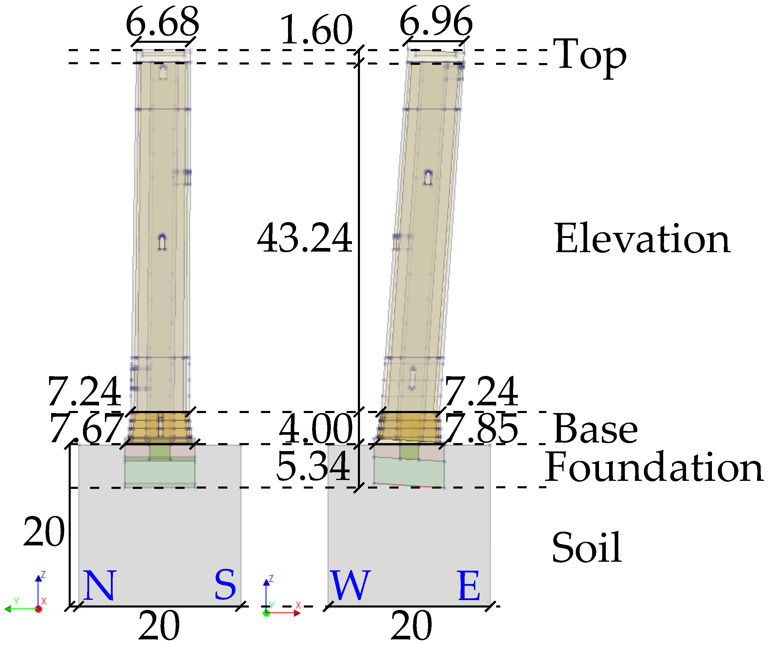
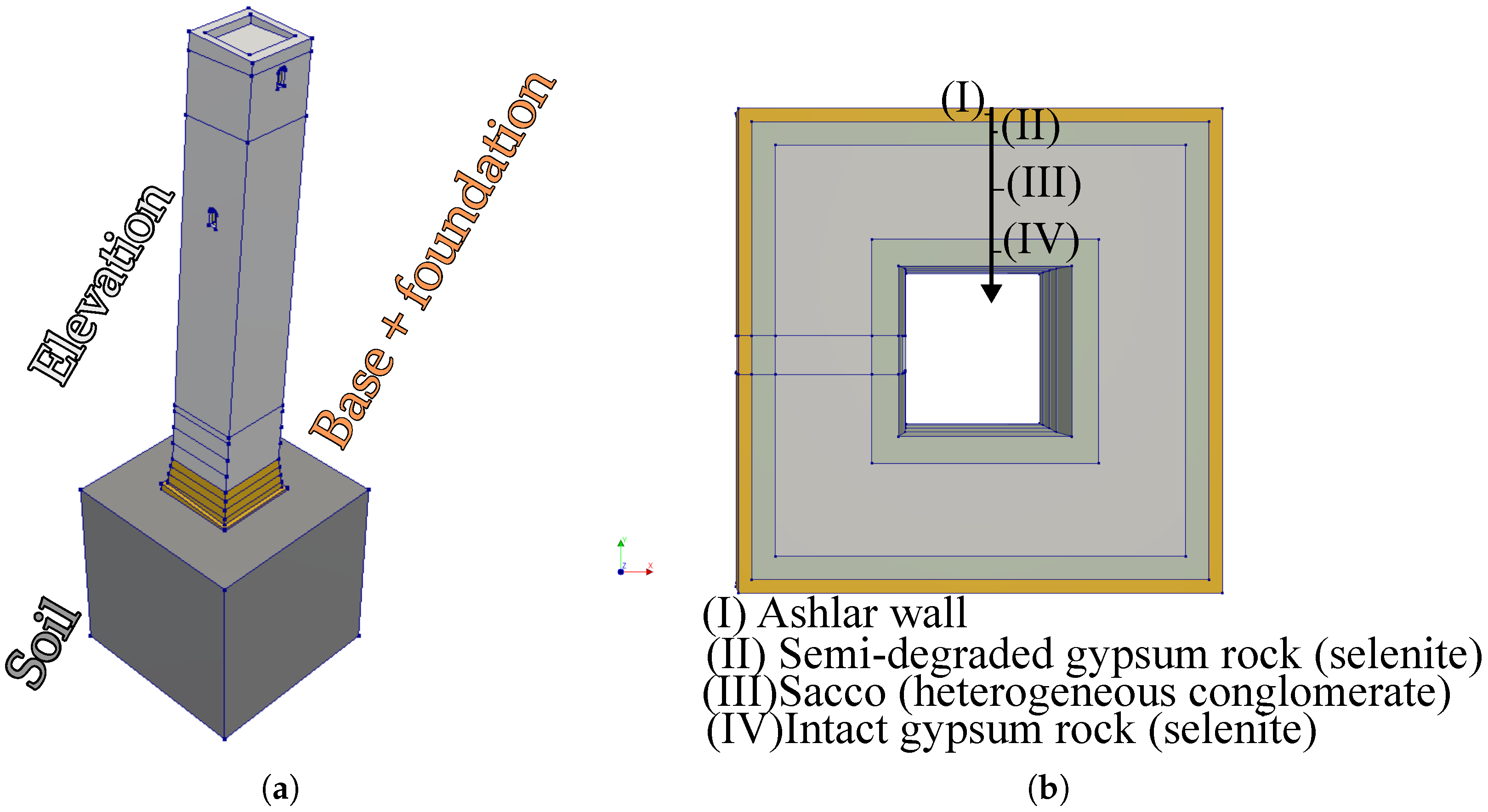
A 3D finite element model was developed utilizing the DIANA commercial package (https://dianafea.com/, accessed 27 October 2025). The computational mesh consists predominantly of quadratic brick and wedge elements, for a total of around 200,000 elements and 600,000 nodes. Mesh refinement strategies varied across different structural regions. In the elevation, an element size of 1 m was adopted (with the exception of the region close to the base, where the element size was set to 0.5 m). In both in the base and foundation, element size was set to 0.2 m, while in the soil a coarser discretization of 2 m was used. The base of the tower was modeled with four layers: two outer selenite layers, an intermediate infill (“sacco”), and an inner selenite layer. The outermost layer of selenite was discretized with one element, while the second exterior layer of selenite was modeled with two brick elements, for a total of three elements and seven nodes through the thickness. For the internal selenite layer, two elements were used through the thickness. West and south views of the geometry of the model in DIANA, with its dimensions, can be seen in Figure 5, while the geometry of the model, with the inner layers, is shown in Figure 6.

The Smeared Cracking and creep models represent the non-recoverable deformation mechanics of the tower and are associated with long-term damage.

Regarding boundary conditions, the soil domain was constrained at its lateral and bottom boundaries to prevent rigid body motion, while allowing deformation compatible with the applied loading conditions. Moreover, all contacts in the model (including soil–foundation) were set as bonded, i.e., no relative displacement was allowed. The additional inclination of the tower was introduced by imposing progressive rotational displacements at the base of the foundation, simulating differential settlement and/or degradation of the foundation system.

The finite element model assumes fully bonded interfaces and employs isotropic material properties for the masonry layers. This could affect the intensity of the cracking observed due to possible over-stiffness in the structure. The influence of other, more flexible contact formulations is to be investigated in future works. These would be interesting to consider—for example, the flexibility of the terrain and soil–foundation interaction. Moreover, a more realistic crack field could possibly be obtained with the consideration of material uncertainty—for example, using random fields of material properties (this capability is present in DIANA FEA) and other probabilistic formulations [14]—or using Monte Carlo simulations, for example, the one adopted in [15] for the seismic analysis of masonry buildings where material properties followed a probabilistic definition. The advantage of using these methods is that cracking could be developed in regions with weaker material properties, which could better reproduce the damage pattern observed in situ. What makes this approach interesting is its feasibility, because the state of health of the materials in the base is known in some cases from previous investigations [2,3].

1.5.1. Smeared Cracking Simulation

A nonlinear finite element analysis was conducted to study the cracking pattern caused by an increasing tilting scenario of the foundation and to understand what additional inclination could lead to catastrophic failure. The materials on the base of the tower were modelled with a Smeared Cracking approach [16], with a linear curve in tension (which models softening due to crack opening) and a parabolic curve in compression (which models plasticization). The stress–strain relations are based on the fracture energy for tension and on the crushing energy for compression.

The material properties adopted for the FE model were selected based on values available in the literature for historic masonry and gypsum-based materials [9,17,18], and are summarized in

Table 1. Material properties used in the FE model: elastic material properties on top, damage material properties on bottom.

Material	Young’s Modulus (MPa)		Poisson’s Ratio	Mass Density (kg/m3)
Silty clay	150		0.3	1900
Elevation masonry	3500		0.2	1800
Selenite masonry	4000		0.2	2400
Elevation filling	2500		0.2	1700
Base filling	4000		0.2	2200
Material	Tensile Strength (MPa)	Fracture Energy (N/m)	Compressive Strength (MPa)	Crushing Energy (N/m)
Silty clay	-	-	-	-
Elevation masonry	0.35	12.0	3.5	5600
Selenite masonry	0.50	15.4	5.0	8000
Elevation filling	0.2975	10.7	2.975	4760
Base filling	0.60	17.5	6.00	9600

(top for elastic properties and bottom for damage material properties). The fracture energy in tension and the crushing energy in compression govern the post-peak behavior and ensure mesh-objective results.

The model comprised two loading phases. In the first, only the tower’s deadweight was applied. In the second phase, progressive rotations in the direction of existing lean were applied to replicate foundation subsidence and/or base wall deterioration. The analysis targeted a maximum inclination of 5°, selected as representing critical structural conditions.

1.5.2. Creep

Creep is an important factor to take into account in the case of historic structures, which has reportedly been the cause of collapse in towers and churches [19,20]. To account for the effect of creep, a preliminary model was built in DIANA considering viscoelastic behavior. The model was built considering a generalized Maxwell material model (a parallel arrangement of spring and dashpot elements connected in series). The goal of the model was to offer an assessment of the evolution of the strains in the base, which could lead to collapse. In particular, as strains in the base continue to grow, so does the tower’s lean, causing material instability and subsequent failure.

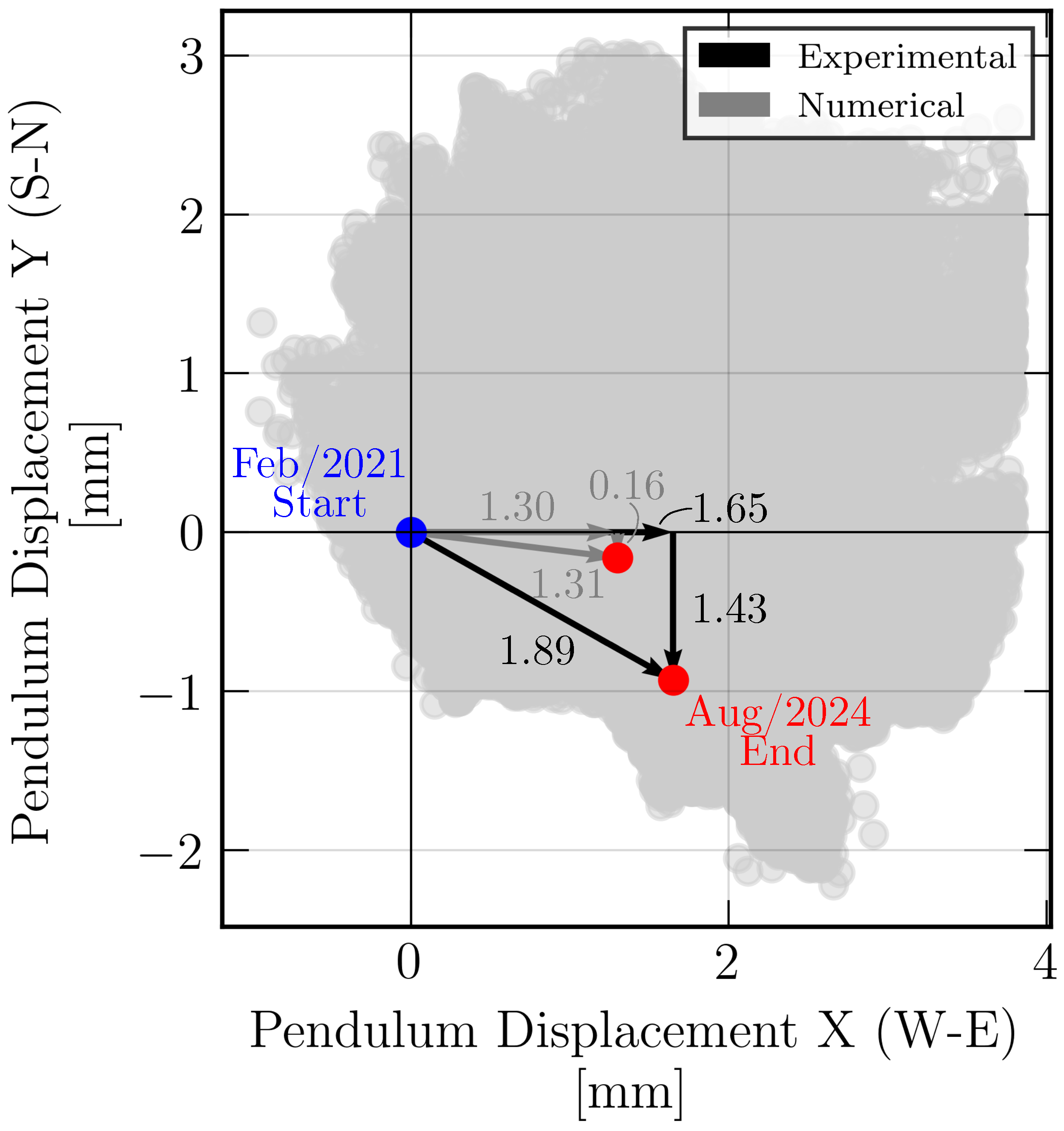
The availability of historical experimental data about the Garisenda poses a challenge for modeling the evolution of its lean with respect to time, as there are not many sources in the literature that point to precise values [21,22]. In this sense, experimental data from the pendulum in recent years (from 02/2021 to 08/2024) made it possible to account for a non-recovered (or permanent) displacement of the top in the present study.

To simulate secondary creep behavior, with an approximately constant viscous strain rate, a viscoelastic model was adopted. Model parameters were calibrated to ensure that primary creep developed during construction phases and that the current deformation rate matched, as closely as possible, experimentally measured values. Specifically, an approximate 1.7 mm displacement increase at the tower summit (in the east direction) was recorded over the preceding 3.5 years. This was accomplished through a five-element Maxwell chain model (comprising one elastic spring element and four spring–dashpot pairs). Obviously, a better approximation of the true secondary creep requires a viscoplastic approach, which is currently under investigation.

The parameters of the viscoelastic model were calibrated to reproduce the experimentally observed long-term displacement trend measured by the pendulum; the calibrated parameters are reported in

Table 2. Viscoelastic chain properties.

	Young’s Modulus (MPa)
Relaxation Time	Selenite Masonry	Base Filling	Elevation Filling
0	4.00 $\times {10}^3$	4.00 $\times {10}^3$	2.50 $\times {10}^3$
1.00 $\times {10}^3$	5.00 $\times {10}^3$	5.00 $\times {10}^3$	5.00 $\times {10}^3$
1.00 $\times {10}^4$	5.00 $\times {10}^4$	5.00 $\times {10}^4$	5.00 $\times {10}^4$
1.00 $\times {10}^5$	5.00 $\times {10}^5$	5.00 $\times {10}^5$	5.00 $\times {10}^5$
1.00 $\times {10}^6$	2.75 $\times {10}^6$	2.75 $\times {10}^6$	2.75 $\times {10}^6$

.

The relaxation times and Young’s modulus for the second to the fourth chains was the same; the only difference was in Young’s modulus of the first chain, that represents the long-term (or static) behavior. It was set equal to the one reported in Table 1 for each material. As mentioned previously, since the model was calibrated to display a coherent behavior with the displacement trend recorded by the pendulum in recent years, it is best suited to the study of mechanical behavior considering a short scale of time. In this sense, while the adopted viscoelastic formulation captures the main features of secondary creep, more advanced viscoplastic or anisotropic models could further improve the representation of the long-term behavior.

2. Results and Discussion

2.1. Principal Component Analysis (PCA)

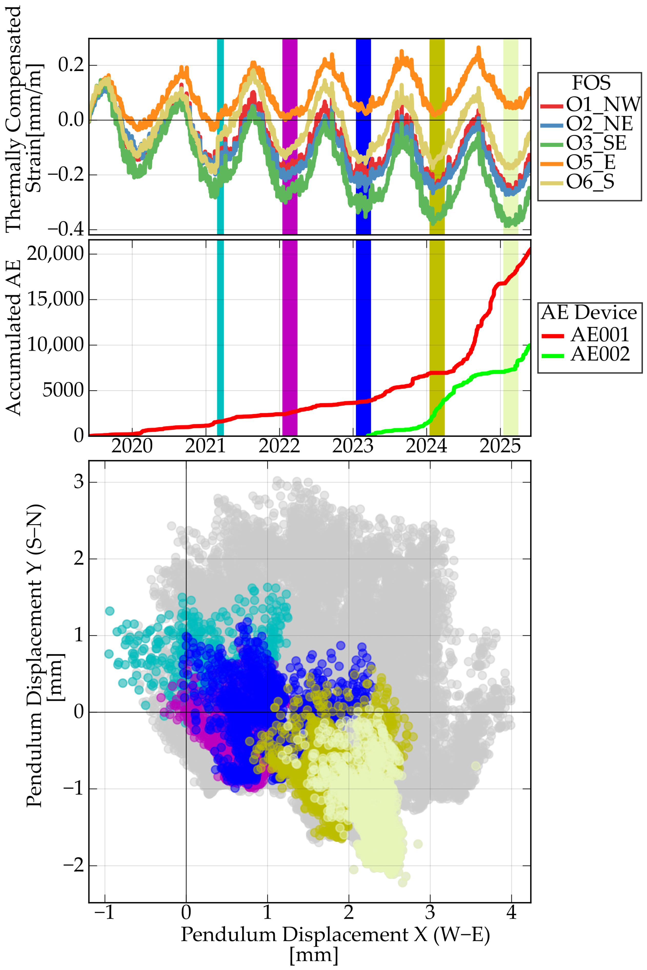
To better understand the need of using PCA in the context of the SHM of the Garisenda Tower, Figure 7 depicts the behavior of the FOS strains, the accumulated number of AE signals, and the pendulum displacements together.

The periods were chosen to be roughly from mid-winter to mid-autumn, to highlight the behavior of the system in winter periods. As can be seen, the global behavior of the pendulum seems to be movement towards the south-east (SE) which is the direction of the leaning. This coincides with surges in AE rate and with global and local minima of FOS strains.

Although a qualitative interpretation of the behavior of the system could be conjectured in this case, a quantitative interpretation of all the available data would be desirable. In such cases, PCA is effective to group together variables that are linked to the same phenomena.

The colored areas represent, in order, the results in the following periods:

• From 25 February 2021, date of the installation of the pendulum, to 31 March 2022 (cyan);
• From 15 January 2022 to 31 March 2022 (magenta);
• From 15 January 2023 to 31 March 2023 (blue);
• From 15 January 2024 to 31 March 2024 (dark yellow);
• From 15 January 2025 to 31 March 2025 (light yellow).

Since cumulative AE variables are monotonic and may dominate long-term variance, they were interpreted together with AE rate and pendulum trends, rather than in isolation. For the present work, the following variables were considered for the PCA:

1.

The hourly acoustic emission rates (number of AE signals per hour) of device AE001 (AE001 Rate);

2.

The hourly acoustic emission rates (number of AE signals per hour) of device AE002 (AE002 Rate);

3.

The accumulated number of signals of device AE001 (Accumulated N of AE Signals—AE001);

4.

The accumulated number of signals of device AE002 (Accumulated N of AE Signals—AE002);

5.

The pendulum displacement in the west–east direction (PDx);

6.

The pendulum displacement in the south–north direction (PDy);

7.

The trend of the pendulum displacement in the west–east direction (Trend PDx);

8.

The trend of the pendulum displacement in the south–north direction (Trend PDy);

9.

The inside temperature of the tower registered by the pendulum (Mean Temperature);

10.

The trend of the inside temperature of the tower registered by the pendulum (Trend Mean Temperature).

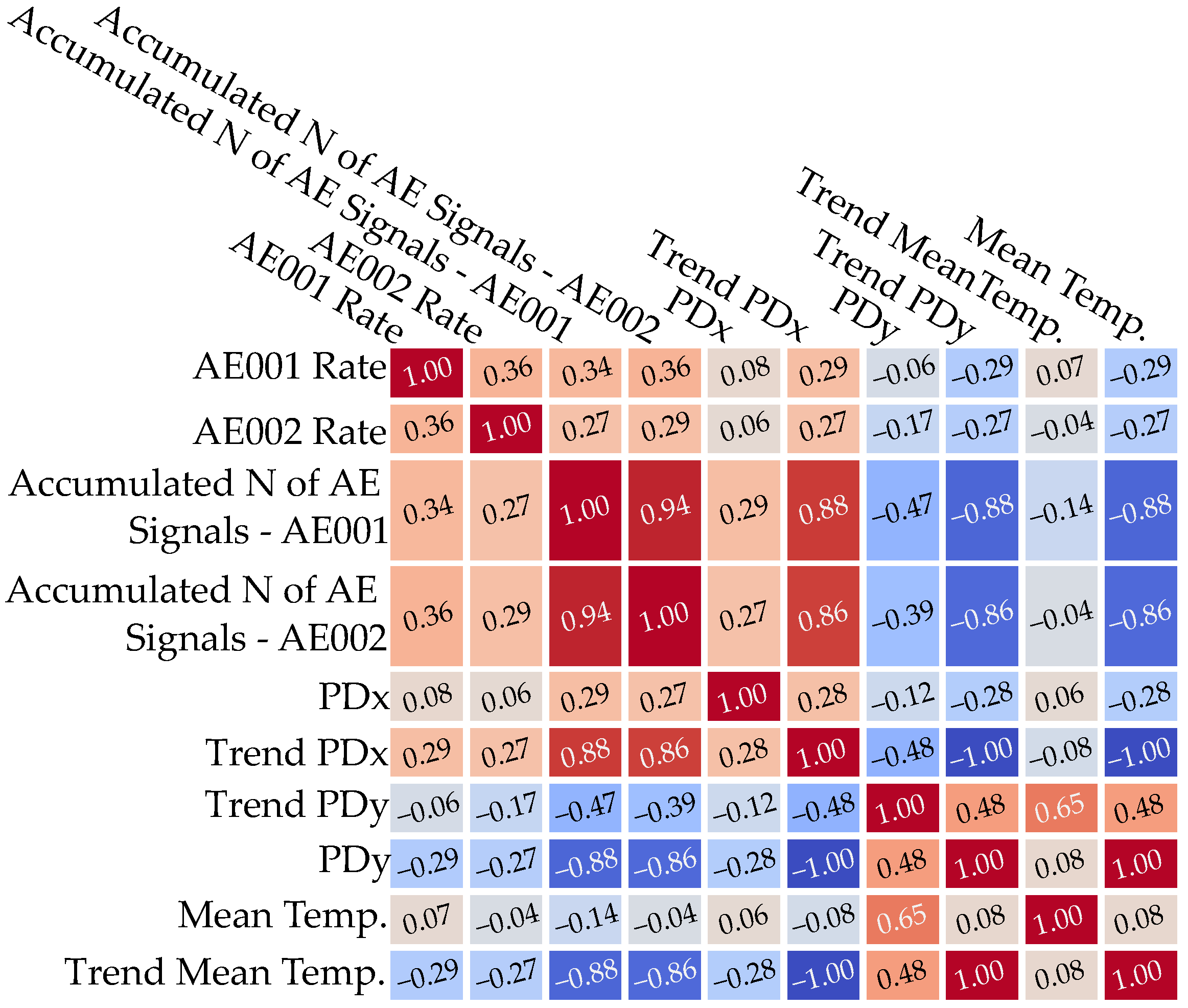
Values were taken from 31 March 2019 to 31 May 2025. As per Equation (1), the variables were standardized and the correlation matrix was built (Figure 8).

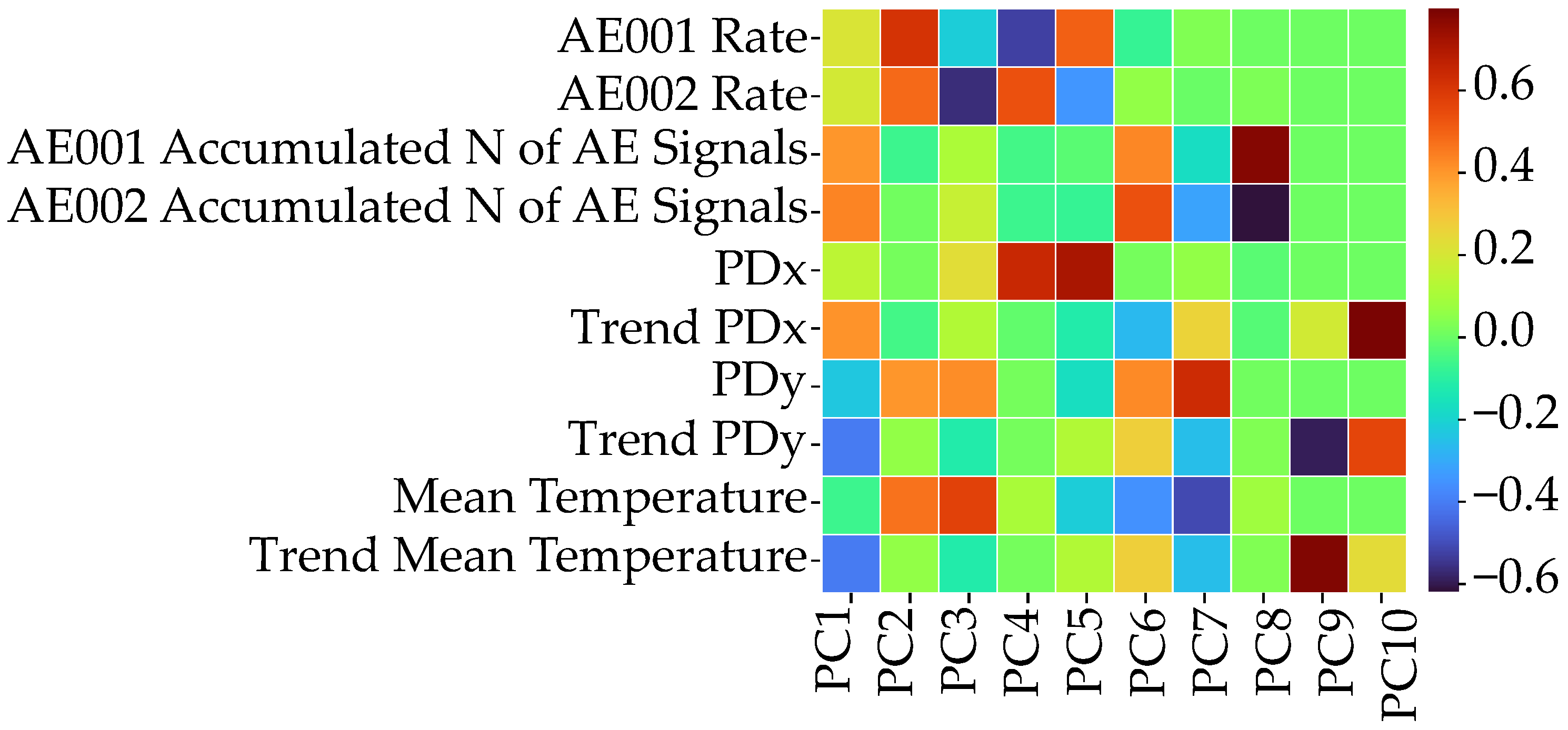
From the correlation matrix, the principal components were determined. Since there are ten variables in the problem, ten principal components were calculated. The principal components, i.e., the impact of each original variable on each PC, are presented in the heatmap shown in Figure 9.

Although physical interpretation of the PCs is always challenging, some patterns can be seen:

• The first PC aggregates accumulated AE, pendulum displacements, and the mean temperature. It is viewed as an indicator of damage caused by the increase in the inclination of the tower (which can also be seen by the pendulum movement).
• The second and third PCs aggregate AE rate (strong correlation for PC2, and strong anti-correlation for PC3), pendulum movement PDy (N-S motion), and mean temperature. They are viewed as changes in damage in the N-S direction due to thermal effects.
• The fourth PC, as with the second and the third, also aggregates AE rate and the pendulum movement (PDx), but this time without the temperature. It is viewed as pure damage caused in the W-E direction.

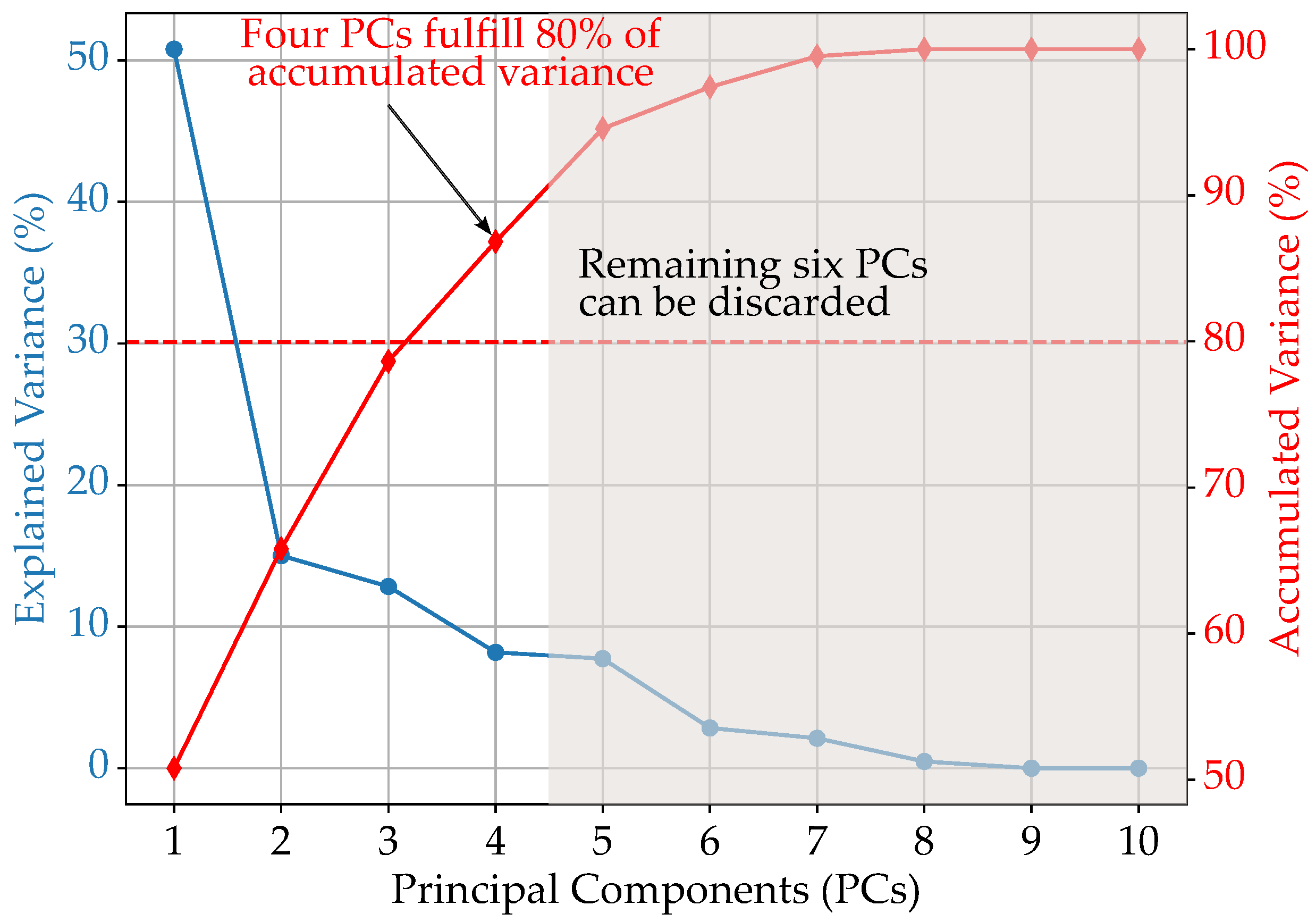
To understand how many principal components were sufficient for the analysis, the cumulative explained variance was calculated, shown in Figure 10. It was seen that the cumulative explained variance of the first four principal components was already higher than 80%, so the last six variables were discarded. In this study, however, attention is focused on the first two PCs. The higher-order components (PC3 and PC4), while not negligible, are associated with more localized effects and are therefore not discussed in detail in this work.

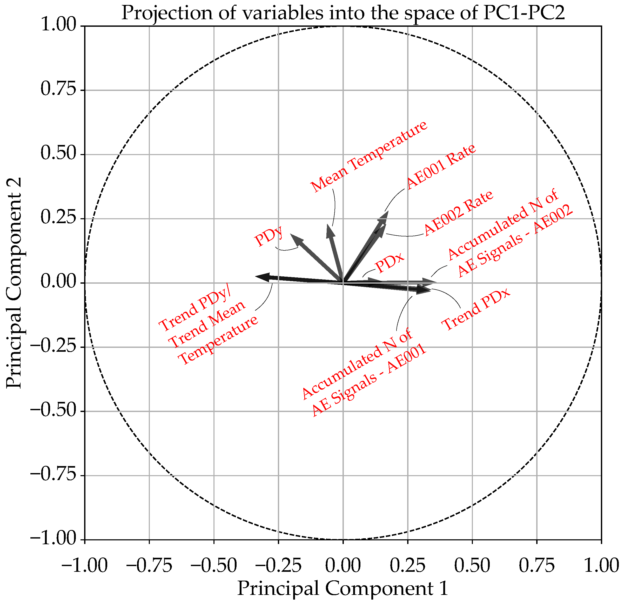
To aid with the interpretation of the results, all variables were projected in the space of PC1-PC2, as can be seen in Figure 11.

It can be seen that:

• The variables PDx, Trend PDx, and both of the accumulated numbers of AE signals point strongly in the direction of PC1, but they point weakly in the direction of PC2. This could mean that they are correlated to damage caused by the pendulum movement in the S-E direction. This is the opposite behavior of the variables Trend PDy and trend mean temperature, which point strongly (and negatively) in the direction of PC1. An interpretation of this fact would be that, when temperatures and PDy increase, the damage related to the movement of the pendulum decreases.
• The AE rates point in the direction both of PC1 and PC2, which suggests that they are correlated to damage due to pendulum motion, specifically in the N-S direction. Interestingly, the AE rates seem to be more sensitive to the damage due to the pendulum movement in the N-S direction, as they point more in the direction of PC2 than in the direction of PC1. The variables PDy and mean temperature point in the direction of PC2, but point in the negative direction of PC1. This reflects that they are correlated to damage in the N-S direction (PC2), but anti-correlated to the damage considering the overall pendulum movement. An interpretation of this fact would be that, when temperatures and PDy increase, the overall effect of damage decreases, while increasing in the N-S direction, as if the damage shifted from W-E to N-S movement.

These interpretations of the principal components are supported by the observation of specific time windows highlighted in Figure 7, where coherent variations in pendulum displacement, acoustic emission activity, and temperature are observed. During these periods, the projection of the variables in the PC1–PC2 space confirms the link between structural movements and damage-related acoustic activity. Possible time-lag effects between temperature variations, pendulum movements, and acoustic emission activity will be investigated in future work.

2.2. Smeared Cracking and Viscoelastic Creep

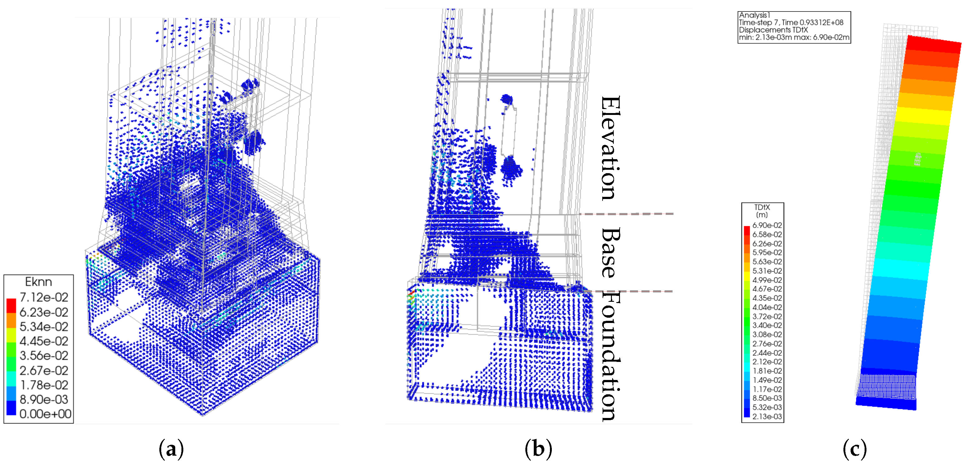
The numerical analysis converged up to an additional base rotation of approximately 2.6°. Beyond this value, convergence could not be achieved due to the development of diffuse cracking and strain localization, which can be interpreted as a physically meaningful indication of structural instability rather than a purely numerical issue. Figure 12a shows the diffused cracking pattern in the lower region of the tower, with the region under tension (closer to the entrance) being apparently the most affected.

If we consider a purely rigid body rotation, the displacement at the top would be around $48\mathrm{m}\times tan(2.6^{\circ })=2.18\mathrm{m}$. In the numerical model, the total displacement at the top is around 3.39 m, which corresponds to 2.18 m of rigid rotation and thus 1.21 m of rotation due to deformable effects. It is noticeable that 3.39 m is is very close to the current lean of the tower of about 3.2 m. If we consider only the lean due to elastic effects, 1.21 m, the value is still not negligible. As such, this configuration is indicative of a kind of upper bound for failure due to tilting.

It is interesting to draw a parallel between the numerical results (in terms of the Smeared Cracking) and the in situ results (in terms of the PCA). Diffused cracking occurs throughout the base, most notably on the side opposed to the leaning (in tension). The damage in the numerical model mirrors the damage caused by the increase in the lean of the tower as seen by PC1, and to damage in the W-E direction by PC4.

In relation to the viscoelastic creep model, the displacement in the east direction is shown in Figure 12b. Additional tilting clearly occurs in the presence of viscous deformation. A comparison between experimental and numerical results is presented in Figure 13.

The creep model built in DIANA reflects well the long-term behavior observed experimentally in the tower, at least considering the displacement in the east direction. The behavior still has room for improvement in the north–south direction.

Both the Smeared Cracking and the viscoelastic creep models were built to study the possible effect of an increase in lean—in the case of the Smeared Cracking model the focus was the soil settlement, whereas in the viscoelastic creep model the focus was the tower structure, and as such they should be seen as complementary. In fact, they aim to investigate the same damage mechanisms (an increase in lean) from different perspectives. Although in this work they were presented separately, future works could combine both viscoelastic creep and Smeared Cracking formulations together, to reflect cracking which could arise from long-term material effects, which is expected.

The consideration of phenomena such as (visco)plastic behavior, or anisotropic viscoelastic models [23,24], could help better model the mechanical configuration of the tower.

3. Conclusions

The present work consisted of combining experimental methods (AE devices, FOS strings, an electromechanical pendulum) and numerical methods (Principal Component Analysis and nonlinear FEM models considering Smeared Cracking and viscoelasticity) to study the damage in the base of the Garisenda Tower.

The Principal Component Analysis effectively reduces complex datasets from AE signals, temperature variation, and pendulum movements, revealing key damage patterns and directional shifts in structural stress, particularly highlighting damage in N-S versus W-E directions.

The increasing tilting scenario using the Smeared Cracking approach highlights that catastrophic collapse could occur around an additional 2.6° of tilt (to be added to the current 4°), with an additional top displacement of 3.5 m (to be added to the current 3.2 m). In general, cracking starts and propagates more in the region under tension (closer to the entrance).

Finally, the creep analysis presents an approach to calibrating viscoelastic parameters from in situ data. It also highlights how viscous effects could play a role in the increase in lean, leading to instability.

Further studies could focus on extending the PCA to include data from other monitoring devices (for example, FOSs) and enhancing the creep model to take into account phenomena such as anisotropy, plasticity and viscoplasticity.