Article

Bridge Network Seismic Risk Assessment Using ShakeMap/HAZUS with Dynamic Traffic Modeling

1
Department of Civil and Environmental Engineering, University of Utah, Salt Lake City, UT 84112, USA
2
School of Civil Engineering, University College Dublin, Dublin D04V1W8, Ireland
3
Department of Civil Engineering, Middle East Technical University, 06800 Ankara, Turkey
*
Author to whom correspondence should be addressed.
Infrastructures 2022, 7(10), 131; https://doi.org/10.3390/infrastructures7100131
Submission received: 7 August 2022 / Revised: 24 September 2022 / Accepted: 26 September 2022 / Published: 1 October 2022
(This article belongs to the Topic Resilience of Interdependent Urban Systems)

Abstract

:
Bridge infrastructures are critical nodes in a transportation network. In earthquake-prone areas, seismic performance assessment of infrastructure is essential to identify, retrofit, reconstruct, or, if necessary, demolish the infrastructure systems based on optimal decision-making processes. As one of the crucial components of the transportation network, any bridge failure would impede the post-earthquake rescue operation. Not only the failure of such high-risk critical components during an extreme event can lead to significant direct damages, but it also affects the transportation road network. The consequences of these secondary effects can easily lead to congestion and long queues if the performance of the transportation system before or after an event was not analyzed. These indirect losses can be more prominent compared to the actual damage to bridges. This paper brings about seismic performance assessment for the Cyprus transportation network from which the decision-making platform can be modeled and implemented. This study employs a seismic hazard analysis based on generated USGS ShakeMap scenarios for the risk assessment of the transportation network. Furthermore, identification of the resiliency and vulnerability of the transportation road network is carried out by utilizing the graph theory concept at the network level. Moreover, link performance measures, i.e., traffic modeling of the study region is simulated in a dynamic traffic assignment (DTA) simulation environment. Finally, for earthquake loss analysis of the bridges, the HAZUS loss estimation tool is used. The results of our investigations for three different earthquake scenarios have shown that seismic retrofitting of bridges is a cost-effective measure to reduce the structural and operational losses in the region.

1. Introduction

Earthquakes as a natural disaster can effectively bring parts of or all the transportation network systems, especially in metropolitan areas, to an immediate halt. Underestimating the seismic risks of bridges, one of the essential components in a transportation system, would bring chaos and disorder to the disaster areas. Bridges assist in transporting goods and disaster victims to and from cities and disaster sites. They are one of the elements in search and rescue in post-earthquake operations of critical infrastructures. Therefore, without proper analysis and assessment of the risk associated with bridges, this could undoubtedly cause disruptions to the transportation network and, ultimately, collapse the lifelines of the impacted regions. The efforts on the analysis of past events have considerably improved the proactive decision-making actions taken to reduce the damage of bridges by earthquakes, but there are still cases where they fail [1]. Moreover, bridges are considered spatially dispersed and interconnected structures. Due to their interdependency, therefore, analyzing one bridge would not necessarily provide enough information to propose suggestions and alternatives for the mitigation of future losses.
Seismic risk assessment provides the necessary tools to assess damage before the main event happens. Provided that seismic hazard assessment of the region is well studied, it is possible to minimize the potential losses following a disaster. Basoz and Kiremidjian [2] presented a seismic event timeline (see Figure 1) that shows the actions and plans that need to take place before and after a seismic event. The first action is assessing potential risks through the use of seismic risk assessment tools. Next is the mitigation strategies to reduce risks such as retrofitting bridges and alternative route planning. In this regard, the highway transportation network plays a vital and integral part of such impact assessments. Consequently, the network-based risk assessment methodologies need to be developed and enhanced further to take into consideration the ever-growing and complex transportation network.
With the proliferation of innovative technologies, it is essential to link different fields of studies into a general framework that can be used to provide better and more accurate results by working together synergistically. Disaster risks following a natural hazard can induce a lot of impacts on the vulnerable people and infrastructure of a region, such as the transportation network. Hence, a decision-support system is essential for assessing the risks.
This paper, therefore, aims to bring about a new methodology for assessing seismic risks of the Cyprus transportation network. By utilizing state-of-the-art tools and methods, we try to extend the well-studied seismic hazard analysis used by researchers and scholars and expand it under the umbrella of the Intelligent Transportation Decision Support System for assessing seismic risk. The outcomes of this study hope to open the path into a fully-fledged decision-making platform with real-time network-based risk assessment providing the best mitigation strategies before and after a seismic event.

1.1. HAZUS, GIS-Based Seismic Hazard Assessment Software

Geographical Information System (GIS) constitutes many components. A visually explanatory platform involving GIS manages multiple data from different sources on separate layers allowing simulation and modeling of all data and their influence on one another. GIS and its useful applications in many disciplines, especially in disaster management cases, comes with shortcomings, however. The time, effort, and possibly money that is essential for advanced GIS applications may deter usage of the tools altogether. Applicability constraints clearly can be seen when analyzing earthquake disasters and its implication on the network, which could produce tens of thousands of spatiallynon-uniformly distributed data that can make processing and analyzing a complicated and time-consuming process [3]. GIS maps with different layers are available online, but the currency of the information provided may be of concern. Therefore, in some cases where there is a lack of information on GIS maps (e.g., unknown bridge locations or highway network information), one needs to spend hours to acquire these data and import them into the correct location on the maps. In the area of bridge performance assessment, standalone applications of GIS are mostly associated with risk assessment and life-cycle risk analysis. Spatially distributed information along with multiple independent parameters of bridges and networks, call for a management system that could operate and analyze different scenarios. Integrating bridge inventory information with earthquake parameters required to produce fragility curves to determine the bridge damage state as one of the input parameters for initializing spatial analysis is widely used in many studies [4,5,6].
Hazard U.S. (HAZUS) is a general-purpose multi-hazard GIS-based loss estimation software. Earthquake loss estimation methods of HAZUS is heavily used by the locals, states, and regional officials in the U.S. as a state-of-the-art decision support software. Development of earthquake hazard mitigation strategies, development of contingency planning measures, and finally, the anticipation of the nature and scope of response and recovery efforts are some of the pre-earthquake applications of HAZUS. It can also be used for post-earthquake analysis for the projection of immediate economic impact assessment and long-term reconstruction plans. One of the new additions to HAZUS was the ability to import ShakeMap data for rapid post-earthquake loss estimation in the affected region. ShakeMap can provide deterministic seismic hazard maps that are used to predict the shaking intensities of earthquakes. The risk assessment results that HAZUS provides are vast in terms of both direct and indirect losses.

1.2. Travel Time Loss Estimation with Dynamic Traffic Modeling

One of the outcomes of this research is to show how damaged bridges in the transportation network can significantly influence the travel time and traffic planning. Travel forecasting models are widely used in transportation planning. They qualitatively and quantitatively evaluate the impacts of future changes in the transportation network [7]. The mesoscopic simulation of the network can share a great deal of information on how individual users choose their paths and what determines their decision on changing routes. dynamic traffic assignment (DTA) modeling can perform such analysis with varying degrees of accuracy, provided that enough information is used to support the simulation. By leveraging the potential of DTA, we have a better insight into what would happen when some bridges completely fail or have reduced capacity due to a decrease in serviceability.

1.3. Objectives

We are primarily interested in modeling the transportation network of Cyprus, and in particular, the performance of such a network under earthquake hazards. The goal of our study is to determine the most critical components in the network and provide alternative solutions or measures to reduce the impacts of risk associated with earthquake hazards. We will apply what we described in the brief introduction of our study in the western part of Cyprus, which includes 20 historical as well as newly built bridges. Therefore, the objectives of this paper are:
  • To develop the seismic hazard maps for scenario-based earthquake analysis.
  • To analyze the structural integrity of the transportation network by employing graph theory.
  • To simulate the dynamic traffic assignment for travel time loss purposes.
The first significant contribution of this paper is the fact that there have been no case studies on a national scale on the transportation network of Cyprus. Most prior works have dealt with ground motion probabilistic assessment of the region. We extend their work and find the risk associated with the results from their studies. The methods used to derive the assessment of the transportation network can also be used in other hazards analyses, such as flood hazards. Furthermore, we incorporate dynamic traffic analysis (DTA) as part of our study for travel time estimation. There have been few works that leveraged DTA in their analyses for risk assessment of the transportation network. We also demonstrate the tractability of adapting HAZUS for our case study.

2. Literature Review

2.1. Seismic Risk Assessment

Evaluation of any risk in civil infrastructural systems, especially those that are critical to the function of a city, is an important task. One area where this assessment is crucial is in the transportation network system, which includes bridges and roadways. Seismic risk assessment requires evaluating every individual component of the network system and then the system as a whole [8]. Understandably, under the umbrella of sustainability and the risk associated with seismic damages, one needs to understand the overall predisposition to social, environmental, political, and economic losses [9,10,11]. The objective of seismic risk assessment is to provide a decision-making platform that can be used as a guide in mitigation scenarios to alleviate the losses during a disaster. Overall system resiliency is a challenge that needs to be addressed in every assessment scenario. The issue with today’s transportation network system is the interdependency and interconnectivity of the transportation system [1,12]. One failed component in the network can significantly influence the functionality of the whole system.
To address some of the issues discussed above, the authors in [12] developed a risk assessment software that takes into account the resiliency of the transportation network. This tool was created to overcome the existing issues with other assessment strategies such as lack of including indirect cost, assumption of deterministic scenarios, and those where no quantification of the resiliency was made. In the work by [13], the authors proposed a seismic risk assessment model for bridges in Charleston, South Carolina. They assessed the risk only in terms of direct losses.
Fixed or variable traffic demand may reduce and impair the highway traffic carrying capacity and influence the network functionality. Variable traffic demand, compared to fixed demand better reflects the real-life scenario. The authors in [14] carried out a thorough analysis of the post-earthquake travel characteristics. Their method was proven to be more effective than the conventional approaches in transportation modeling. Similarly, the authors in [10] introduced a framework to include post-disaster traffic demand in emergency conditions. Moreover, it was shown that network topological features reflect a different aspect of the traffic flow of the bridge network. The works in [15] and [5] discussed the estimation of the direct and indirect losses to bridges in the St. Louis metropolitan area. For the worst-case scenario in the direct loss estimation case, the associated indirect cost was found to be more than half of the cost of the direst losses, clearly indicating the importance of evaluating this form of loss.
In most research papers, bridge performance assessment under seismic activities is only evaluated based on one hazard, generally ground shaking. However, multi-hazard assessment is also very popular. A complete risk assessment methodology was presented in [16] where the authors expanded their approach and included liquefication and landslide hazards in addition to ground shaking. It was found that the loss due to traffic delay was found to be higher than the cost of repairing damaged bridges. A similar paper [8] showed that for a single deterministic earthquake scenario of a magnitude M7.0, liquefaction accounted for the most substantial damage to the transportation network. The authors also found that for their variable traffic demand case, they observed lower travel time delay.
The study [11] evaluated the socio-economic cost of bridges for two sets of scenarios, before or after the seismic retrofit. They evaluated the social cost in terms of travel delay with the assumption of a reduction in traffic flow after an earthquake. It was found that retrofitting was more cost-effective for lower discount rates and bridges with higher average service life. A similar study in [17] was presented, albeit with the focus only on travel time delay for deciding whether or not to retrofit bridges. The authors indicated the significance of bridge retrofitting on reducing travel time after an earthquake event. The authors in [18] illustrated a seismic risk assessment of both industrial plants and tunnels and bridges of the Friuli–Venezia Giulia highway network in Italy. In their study, unlike other papers where they evaluate the losses in dollar figures, relied on a simple probability estimate percentage for a 50-year return period ground motion.

2.2. HAZUS International Adaptations, Seismic Risk Assessment Tools

HAZUS was initially intended only for risk assessment of different hazards in U.S. regions. However, with further developments, transitioning to a more versatile data management scheme, and the introduction of HAZUS specific open-source tools, it is now easier to implement HAZUS in different regions around the world [19]. At the current stage, the adaptation of international regions to HAZUS requires extensive data collection, in addition to conforming to the original data format. This can prove to be difficult for those regions that do not follow exact HAZUS definitions of administrative boundaries, hazard-specific fragility classifications, and much more.
An example of one use-case of HAZUS software in regions other than the U.S. was discussed in [20]. The authors investigated the sensitivity of the Canadian version of HAZUS for flood risk assessment. Another example was presented in [21]. The authors in this paper studied the risk assessment of hospitals in the city of Yazd in Iran.
Other than HAZUS, different risk assessment tools are continually being developed all around the world. AFAD-RED is Turkey’s first national operational tool for the prevention, preparedness, and response to seismic hazards. The open-source OpenQuake project as part of the Global Earthquake Model (GEM) initiated a worldwide collaborative effort to bring state-of-the-art science behind seismic risk assessment tools developed by different organizations and individual researchers to a common, uniform, and open standard way of communicating earthquake risks [22]. The OpenQuake engine is now the primary tool used by new risk analysis platforms and large-scale real case implementations such as the Euro-Mediterranean Seismic Hazard Model (ESHM13) European Union project [23]. CAPRA is a probabilistic risk assessment system. The modules available in the CARPA platform are capable of both hazard and climate change risk analysis. SELENA is a tool developed by the Norwegian seismic array (NORSAR) in Kjeller for Norway. Ergo is another open-source seismic risk assessment platform and application developed by the National Center for Supercomputing Applications at the University of Illinois at Urbana-Champaign. This tool is based on the core functionalities of the old MAEViz platform. A complete list of new and old tools used for seismic hazard and risk assessment is provided in [24].

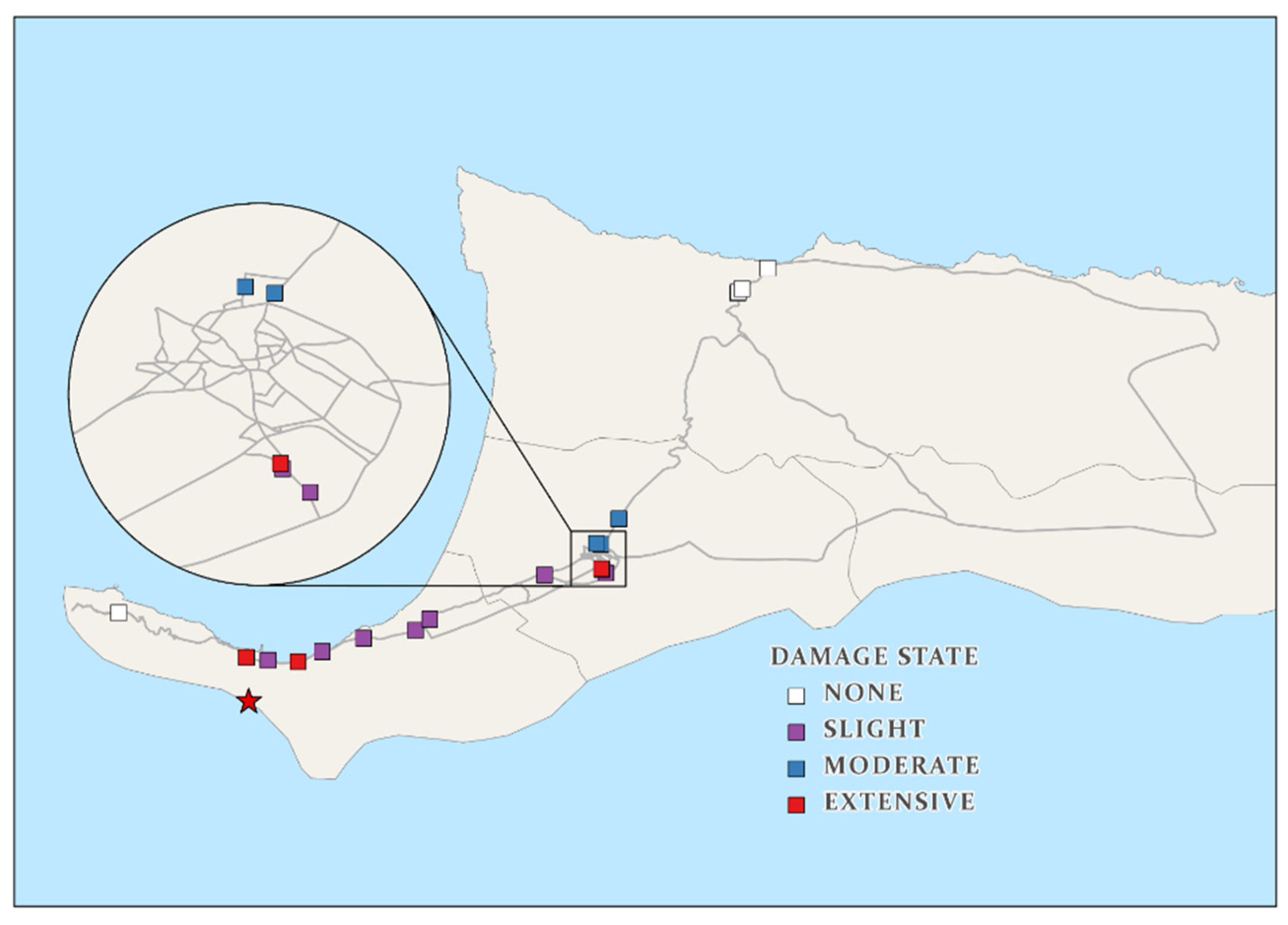
3. Seismic Hazard Analysis of Northern Cyprus

3.1. Seismicity of Cyprus

Just like any other part of the Mediterranean region, there have been historical records of devasting earthquakes in Cyprus dating back as far as 1500 B.C. [23]. Southern Cyprus started implementing modern instrumentation of seismometers (Cyprus Broadband Seismological Network) in 1997 [25], shortly followed by Northern Cyprus. In total, there are 13 seismometers (5 in the northern part) with different sampling rates ranging from 50 Hz to 100 Hz at different orientations operating 24 h. Figure 2 shows the distribution of these seismometers in Cyprus.
There have been several attempts in identifying the fault lines as well as the seismic sources of Cyprus with varying degrees of details. Two recent studies, namely the work by Cagnan and Tanircan [23] in 2010 and the 2013 Euro-Mediterranean Seismic Hazard Model (ESHM13) European Union project [26], attempted to model the seismic hazard of Cyprus. The two projects were based on the tectonic map of the region, which was developed by the United States Geological Survey (USGS) [27] in 2000 after the work by Barka and Reilinger [28]. Given that many earthquake epicenters are shallow, i.e., originating within 60 km of the Earth’s other surface, this warns for taking necessary measures to ensure the safety of the region in terms of the possible earthquake hazards. The ESHM13 study resulted in identifying the faults capable of generating earthquakes with magnitude M5.5 or larger. For the case of Cyprus, it has been shown that the regional faults can generate magnitudes larger than M6.0. Figure 3 illustrates the faults with the maximum possible magnitude and the distribution of earthquakes from 1956 to 2020 collected from the USGS earthquake catalog.

3.2. Generating ShakeMap Data for HAZUS

As part of our analysis in HAZUS, we created different scenarios based on different magnitudes, depths, and different Ground Motion Prediction Equations (GMPEs). To achieve this, we created ShakeMap scenario data for our region. ShakeMap is developed by USGS written in Python programming language. With the geological information, ShakeMap can automatically generate shaking and intensity maps in real-time when an earthquake occurs. It is one of the emergency tools used by many agencies in the U.S. for rapid loss estimation. ShakeMap can produce different Intensity Measures (IM) such as, peak ground acceleration (PGA), peak ground velocity (PGV), and spectral acceleration (SA) at 0.3, 1.0 and 3.0 s, respectively. These are precisely the default IM requirements of the HAZUS loss estimation methodology. We used three different GMPEs (MultiGMPE analysis) developed by Boore and Atkinson in 2008 [29], Campbell and Bozorgnia in 2014 [30], and finally, Akkar and Bommer in 2010 [31] when creating ShakeMap data. To account for the use of multiple GMPEs, we incorporated weights for each GMPE such that Boore and Atkinson [29], Campbell and Bozorgnia [30], and Akkar and Bommer [31] were each assigned with the weights of 0.4, 0.4 and 0.2, respectively. The two reasons for the selection of the above weights and GMPEs are that first, these models are developed for shallow earthquakes, as is the case of our region and second, weights are distributed based on more recent and up-to-date regional data, as suggested in [23].
The site condition of majority of Cyprus shows high shear wave velocity (see [32]), and the higher the velocity, the less the ground shaking amplification. Hence for observing any damage, earthquake magnitudes of M5.0 or above are required. For the current active fault lines of Cyprus, we can expect magnitudes of up to M7.4 for the western part of Cyprus at depths less than or equal to 70 km. It should be noted that the direction taken in generating shaking distributions under scenario modeling is not as complex and is more uniform compared with real event shaking maps. In real shaking intensity distributions, 2D and 3D wave propagation, basin-edge effects, and other complex site effects are usually accounted for. Nevertheless, using this tool we can analyze different hazard levels for better preparedness and emergency response.

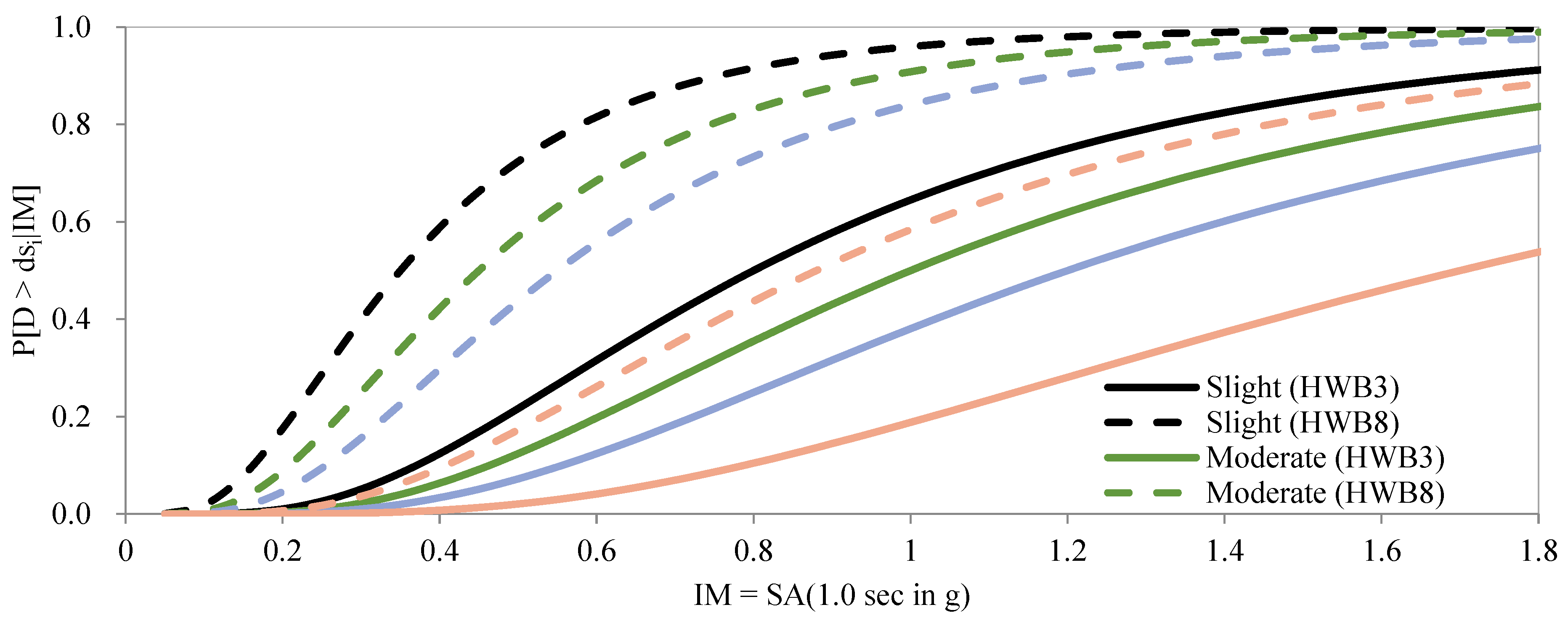
3.3. Seismic Risk Assessment through Fragility Analysis of Bridges

In contrast to the seismic hazard analysis discussed previously, seismic risk assessment describes the potential for damages or losses that a region is prone to experiencing after a seismic event. They can also be defined as the integrated product of the seismic hazard, that determines the value and fragility of assets [33]. This link between ground motion intensity and structural damage is related by the fragility functions. They are also known as damage functions that are usually represented by conditional cumulative log-normal distribution functions, that are depicted as curves for a given level of damage. These curves are the key input for seismic risk assessment for evaluating bridges and corresponding loss of serviceability for a defined damage level. Depending on the form of fragility analysis, the conditional probability that a given structure exceeds the prescribed damage limit state ( d s ) is usually defined as:
P [ d s i | x = I M ] = Φ [ 1 β d s l n ( I M S m e d i a n ) ]
where, I M represents the intensity measure, e.g., PGA; Φ is the standard log-normal cumulative distribution function; β d s indicates the log-normal standard deviation of I M ; and S m e d i a n denotes the median (or expected value) of the I M . According to HAZUS methodology [34], bridge damage states can be summarized in Table 1.
In HAZUS, 28 primary bridge classifications are defined for the entire U.S. As a result, for the four damage limits defined in Table 1, 112 fragility curves were developed according to the study in [35]. These ‘standard’ curves have to be modified to reflect the characteristics of the bridge such as 2-dimensional piers’ capacity to 3-dimensional arch action in the deck K 3 D , shape factor K s h a p e , and finally skewness of the bridge K s k e w through a scaling procedure defined in the HAZUS manual. These discrete damage state probabilities are subjective and can vary depending on the methodology used. The definition of the damage in terms of the structural losses (cost) for an event m can be defined such that:
D i r e c t   L o s s m = n = 1 # b r i d g e s k = 1 # D S D R k P [ d s n m ] p r o b a b i l t y   o f   b e i n g   i n   a   s p e c i f i c   d a m a g e s t a t e c o m p o u n d e d   d a m a g e   r a t i o   ( D R C ) × R e p a i r   C o s t   n  
where D R k denotes the damage ratio in terms of the replacement cost. HAZUS defines bounds for each damage state according to the severity of the damage, as shown in Table 2.

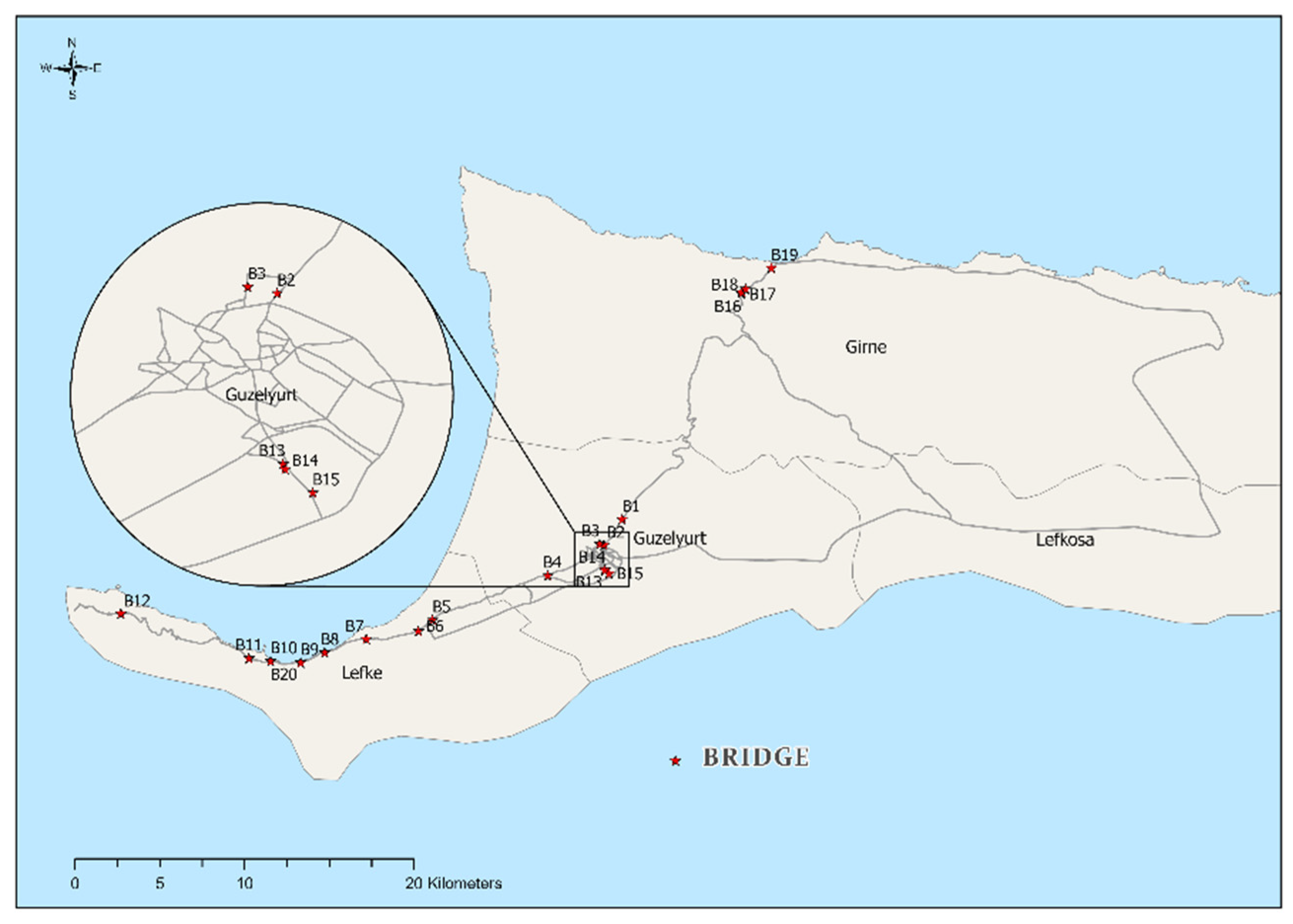
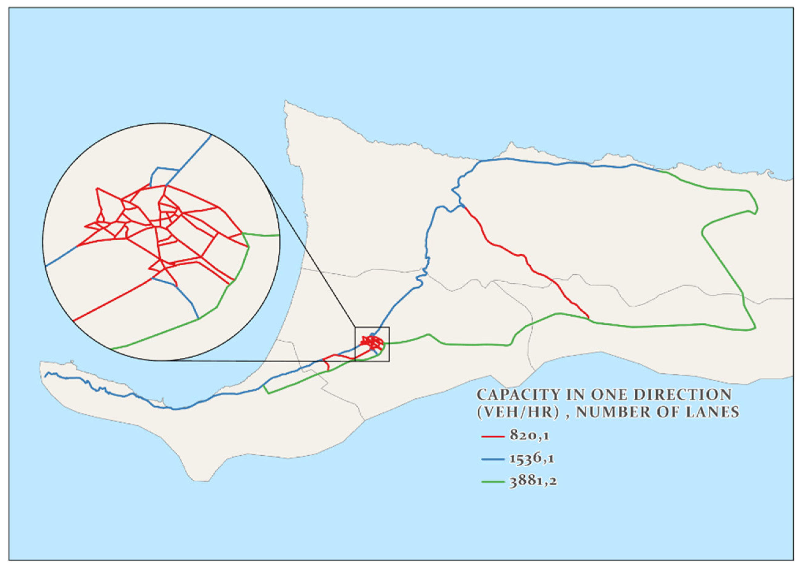
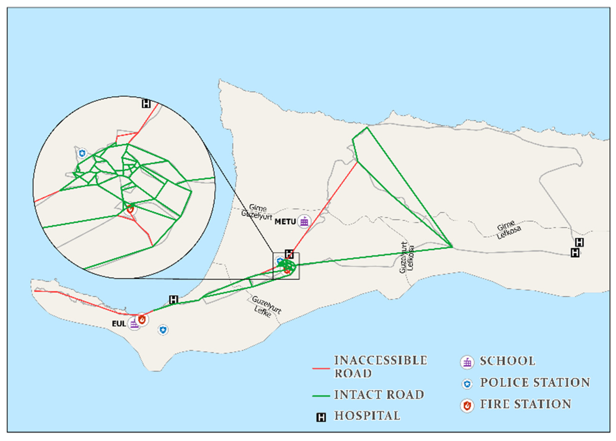
4. The Transportation Network of Northern Cyprus

Bridges are vital components and vulnerable elements in any transportation network [8]. Not only the failure of such high-risk critical components during an extreme event can lead to significant direct damage to the bridge, but it also affects the crucial lifelines connecting the epicenters to other locations. Such indirect damage to the road network can easily lead to congestion and long queues. Therefore, the serviceability of the road network becomes a metric that must be carefully examined in three different categories, (1) travel time delay, (2) network flow capacity and overflow, and (3) the connectivity of the network. In this section, we analyzed the Cyprus road network in terms of its topology, spatial distribution of its components, and the dynamic model of the traffic assignment.

4.1. Network Reliability and Vulnerability

Transportation networks are diverse and sparse. They are considered as interconnected systems where a failure on any link would result in cascaded degradation on the upstream and downstream parts of the network. The relationship between system and network must be understood before evaluating reliability measures. In practice, a system is represented as a network where each individual system’s components are connected in series or parallel. One of the simplest methods of evaluating reliability measures is using binomial distribution where the probability of success “p” is just the network’s reliability. In a series system, the system reliability, R s , becomes R s = i R i ; or the product of the reliabilities of its constituent components. Whereas, in a parallel system, the system’s reliability becomes R s = 1 i ( 1 R i ) ; or the product of the component’s reliability. Here, network connectivity and travel time reliability are the measures that network reliability studies usually consider evaluating the performance of urban road networks [36]. Reliability, in general, is defined as the quality of service that a system offers typically with regard to its degree of stability [37]. Considering rural areas, however, at the regional and national strategic level, reliability measure is often replaced by vulnerability analysis. As an example, consider enhancing the reliability of an urban road network by introducing effective measures to increase the capacity or by creating an alternative route to lessen the burden on a given link. However, considering these selective additions at a provincial level would not necessarily help to increase reliability. These two performance measures are related, but fundamentally, vulnerability analysis becomes an important subject in seismic performance assessment of transportation networks as reliability measures themselves can become vulnerable in severe events. Network resiliency, such as robustness and redundancy, are evaluated based on metrics from graph theory. The network connectivity, loops (redundancy), and robustness are evaluated based on network structural measures at the node and edge levels. For example, the clustering methods and gravity index can be used to provide a simple resiliency measure for the network. Ideally, the resiliency should encompass both structural reliability and traffic flow reliability considering the transportation network characteristics. However, for simplicity and demonstration purposes, only topological vulnerability analysis was carried out in this study.

4.2. Topological Vulnerability Analysis Using Graph Theory

Network analysis, sometimes referred to as graph theory, plays an essential role in determining the efficiency of transportation networks [38]. Graph theory deals with understanding the properties of a set of linked vertices (nodes), V , through edges (links), E . A graph G = ( V , E ) is a simple structural representation of a 2D planar of a real network as illustrated in Figure 4.
One of the first uses of network modeling is measuring network properties [39]. In our study region, the transportation network consists of V   = 98 nodes and E = 134 edges with a total length of about L = 124   km . The network properties are defined for the abstract, i.e., graph version of the network. The Cyprus transportation network, in comparison to other research studies, is less complicated. The intention was to select the most critical nodes such that the network could be kept as simple as possible for future analysis without sacrificing the quality of the results. More in-depth analysis can be performed at the community level, but this is out of the scope of this study.

4.3. Structural Measures and Indices at Network Level

Measuring performance at the network level can enable the analysis of the network and to compare and show the evolution of the transportation network. The following provides additional measures alongside the basic description of the network. Many of the formulations are derived by Kansky [40,41].
Diameter d of the network shows the length of the largest shortest path. A higher δ indicates less linked a network tends to be.
δ ( G ) = max d ( u , v )   f o r   u v
where d ( u , v ) shows the length of the shortest path from vertex u to vertex v .
Number of cycles μ shows the maximum number of independent cycles in a graph. A higher u is an indication of the complexity of the transport system. Index p indicates the number of sub-graphs, usually taken as one.
μ = e v + p
Different indices can be derived to show the complexity of a transportation network and the changes in the structural measures overtime. We only discuss the topological indices for this study. These indices are defined as ratios expressing a relation between two values.
Alpha ( α ), beta ( β ), and gamma ( γ ) indices express the relations between elements of a network. α index indicates a measure of connectivity in terms of cycles in a graph. With the increasing number of links, the ratio will approach to 1, i.e., a fully connected network.
α = μ 2 v 5
β index measures the connectivity in a graph by expressing the ratio of the number of links to nodes. A high β index in complex networks indicates a surplus of link in the network.
β = e v
γ index measures the connectivity in terms of the number of observed links and the number of possible links. Similar to α index, γ index approaching 1 shows a fully connected network.
γ = e 3 ( v 2 )
Eta ( η ) and Pi ( π ) indices express the relations between the network and one of its elements. η index or the measure of average edge shows that with the addition of nodes, e.g., intersections in the network, the shorter the average edge length becomes, thus decreasing the maximum flow q in the network.
η = L ( G ) e
π index shows the relation between the total length of a graph and its diameter. A higher length of the network tends to show a more complicated transportation network; therefore, a higher π index reflects higher degrees of development. It roughly indicates the shape of the network.
π = L ( G ) δ ( G )
The above structural measures and indices often do not reveal the internal structures of a highly complex interconnected transportation network. For this reason, performance measures should also be carried out at the node and link levels. It becomes of the utmost importance while carrying out a vulnerability analysis to have a better understanding of what might happen if a node or link becomes either completely unusable or with less carrying capacity, i.e., reduction in serviceability of the transportation network. The results of the pre-event assessment of the transportation network are provided in Table 3.

4.4. Structural Measures and Node and Edge Level

The abstract network G , with physical connections to the real network, can be evaluated based on system-based vulnerability analysis at the node and edge level [42], giving a better representation of the actual network performance considering the importance of a node at the local or global scale and the effect of weighted links. Local measures are only used in finding metrics with respect to neighboring nodes, whereas, when considering a node’s situation in the whole network, the global measure can better highlight the overall performance. The following discusses some of the structural (topological) vulnerability metrics. The analyses were performed utilizing three different applications: Urban Network Analysis Toolbox for ArcGIS developed by City Form Lab [43], SANET (Spatial Analysis along Network) Standalone Tool V1.0 Beta [44], and Python 3.7 with NetworkX library [45].
Degree of centrality C D or the order of a node in a network simply shows the summation of all its edges. A higher degree indicates the importance of that node. The magnitude of C d is partly a function of the size of the network [46].
C D ( v ) = j = 1 n G ( v , j )
Betweenness centrality C B computes the shortest path between nodes or edges. It finds the fraction of the total number of shortest paths passing through a node v or an edge e . Given a pair of source and target nodes V ( s , t ) , the betweenness centrality is calculated as:
C B ( v ) = s , t V σ ( s , t | v ) σ ( s , t )
C B ( e ) = s , t V σ ( s , t | e ) σ ( s , t )
where σ ( s , t | v ) , and σ ( s , t | v ) indicate the number of paths passing through some node v and some edge e , respectively. Similarly, σ ( s , t ) is the number of shortest paths between ( s , t ) - path .
Closeness centrality C C indicates how close is a node is to all other nodes in the network. It computes the reciprocal of the average shortest path distance to a node. It is defined for a node u as:
C C ( u ) = n 1 v = 1 n 1 d ( u , v )
where n is the number of nodes reachable by u . A higher C C indicates higher centrality. It should be noted that NetworkX algorithms for calculating C C are normalized according to:
n 1 | G | ¯ 1    
Gravity index takes into account the additional factors in the spatial impedance, such as length or other measures [47]. It is primarily used by urban planners to better understand the dynamics and the development of a region. Its primary function is to determine the attractiveness of an area in terms of its accessibility to the other nodes in the network. This index is not a main measure of the performance of a transportation network for the context of this study. Nevertheless, it can still be used as a way to show how a network can be affected if vulnerable nodes or links are removed from the network. The gravity index ( G I ) of a node i with respect to destination j within the graph G given a search radius r is defined as:
G I [ i ] r = j G { i } , d [ i , j ] r W [ j ] e β . d [ i , j ]
The exponential decay e β can be controlled based on the calibration carried out for a specific impedance metric. The exponent β is defined as 0.00217 for the impedance unit in meters [48].
Hotspot analysis of events distributed over a network is one of the fundamental concepts in spatial analysis [49]. One of the most frequently used methods for analyzing distributed points on a network is to estimate the density of the points [50]. Kernel density estimation (KDE) is one of the most common techniques used in discovering hotspots of point-events [51]. Ordinary KDE models such as 2D Planner KDE are not useful in analyzing linear road networks. Hence, an extension to the ordinary KDE, Network KDE (NKDE) was developed [52] such that:
λ s = i = 1 n 1 r k ( d i s r )
where λ s represents the density in location s, and r (bandwidth) indicates the search radius. The kernel function k , defines the distance decay effects or the weight of the distance of a point i to location s . Therefore, the longer the distance, the less weight is applied to calculate the overall density. k can be defined with different models, such as Gaussian, Quadratic, Conic, and many others [52]. Instead of analyzing point-events on a network (e.g., crash zones, crime zones), as is the case for most of the kernel-based analysis, we tried to estimate the density of bridges and intersections for our study region. This way, we can get kernel classes for the whole network that could give a better overall view of the vulnerability of the network when a node (i.e., bridge) is removed from the network. Generally, NKDE analysis is performed over a real network, but to keep the flow consistent, we used the abstract model, i.e., the graph. To perform the NKDE analysis, we used the SANET Standalone tool.

4.5. Link Performance Measures

In the previous sections, we discussed the reachability or the connectivity of the transportation network by analyzing the abstract representation of the study region through different metrics from graph theory. We determined the performance from a structural perspective. However, the real elements in the networks, i.e., the flow of traffic, could also play an important role in the overall network performance before and after an event. By looking at the travel demand and through network flow theory models as well as traffic assignments, we can quantitatively measure the impacts of travel time delays and queues.
Trip assignment simulates vehicular movement through the network given the travel demand and zonal constraints, as well as overall network characteristics (e.g., signalized intersection, link speed, capacity). We can estimate the traffic demand between zones and identify the congestions, travel patterns, effects of link/node removal, and many other measures. Typically, trip assignments work by simulating the minimum path between origin-destination (OD) pairs such that a traveler would always minimize the travel time. Travel time on a network (a measure of link performance) is typically defined by the power function developed by the Bureau of Public Roads (BPR) [53] as:
t = t 0 [ 1 + α ( V C ) β ]
where t indicates the travel time on the network; V and C are the volume and capacity of the link, respectively, and α and β are coefficients calibrated for different free-flow speeds. In general, α = 0.15 , and β = 4 . The free-flow travel time t 0 is defined as:
t 0 = L / v 0
where L is the length of the link, and v 0 is the free-flow speed. In order to realize the performance of the network for the current and future scenarios, the vehicular flow patterns are simulated either by static traffic assignment (STA) or dynamic traffic assignment (DTA) models.

Static vs. Dynamic Traffic Assignment

Traditionally link performance was analyzed by STA methods. In 4-step transportation planning, STA forms the last step of the process, and it is only capable of static roadway condition modeling. It does not consider dynamic routing (time-varying travel conditions), congestion, queue buildup, or spillovers [54,55]. STA does put a limit on the actual flow on the road as it distributes the traffic on the network at the same time. Therefore, the traffic demand would, in some cases, exceed the capacity of the links resulting in an inaccurate estimation of the network’s performance. DTA, on the other hand, considers the fundamental relation between flow, capacity, and density, which in turn provides a more realistic traffic flow pattern. Incorporating the interactions of the road users with the network characteristics, allows for a far better travel time reliability estimation for vulnerable links on the network. For analyzing our study region’s link performance, we incorporated NeXTA DTALite (Network Explorer for Traffic Analysis, Light-weight Dynamic Traffic Assignment Engine) [56]. NeXTA DTALite is a queue-based mesoscopic traffic simulator for travel modeling. Mesoscopic models are typically a middle level between macroscopic and microscopic models. They are used to bridge inconsistencies between the two aforementioned models. In most applications of traffic assignment, the user equilibrium (UE) method is used to optimize the traffic assignment.
According to Wardrop, users (drivers) are selfish (non-cooperative) and have complete knowledge about the network (the path cost). To satisfy the user equilibrium through iterations, the following conditions/assumptions are to be made:
(1)
No user can reduce his/her path cost by switching routes, and
(2)
the route used between the OD pairs have equal and minimum cost (shortest path); the rest of the unused route has greater or equal cost compared to the used path cost.
In NeXTA DTALite, dynamic UE (DUE) is used that generalizes as a nonlinear minimization problem via gap functions and solved through iterations until a UE is reached. Interested readers are recommended to check the detail DUE in [57]. To achieve a precise DTA model in NeXTA DTALite, we required extensive knowledge of the transportation network, including availability to sets of data that are not accessible or infeasible to collect. Therefore, to simplify the task while keeping the necessary level of detail for this study, some of the parameters in the program were kept as the default values according to the standards.

4.6. Inventory and Traffic Data Collection

For this study, we counted the traffic flowing on 20 bridges for 1 h at 15 min intervals during peak hours (see Table 4). This allowed us to estimate the peak hour volume (PHV), peak hourly factor (PHV), average annual daily traffic (AADT) and directional design hour volume (DDHV). Counting was performed during weekdays in fall and spring at random intervals; however, we also observed weekend traffic and concluded that, during the weekend, the traffic was almost half of weekday traffic. Some of the bridges were located on parts of the roadways that did not accommodate traffic often. The links associated with these bridges were not studied unless the links were part of the network that could allow traffic to pass in case of the failures of adjacent links. Table 5 provides the full description of the identified bridges in the study region and Figure 5 depicts the distribution of the bridges over the extent of network under study.
Most of the road network in our study region comprised two-lane roads. While counting the traffic, we included both directions, as suggested in the Highway Capacity Manual (HCM) [58]. In order to perform capacity analysis, we used the two-lane highway definition of the HCM (volume 2, chapter 15) for links where counting was performed. We assigned the majority of roadways as Class III two-lane highways defined in the HCM. If the parameters necessary for capacity calculation were unknown, we used the default values defined in the HCM. NCHRP 387 method [59] was selected for other rural two-way roads where traffic counting was not performed. The network capacity is illustrated in Figure 6.

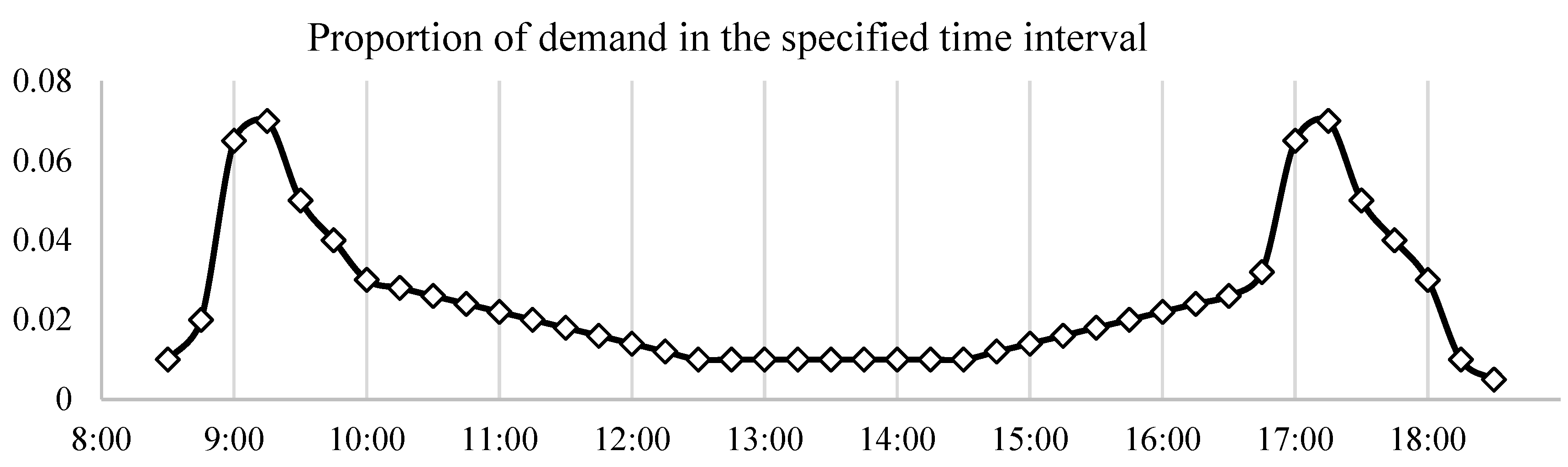
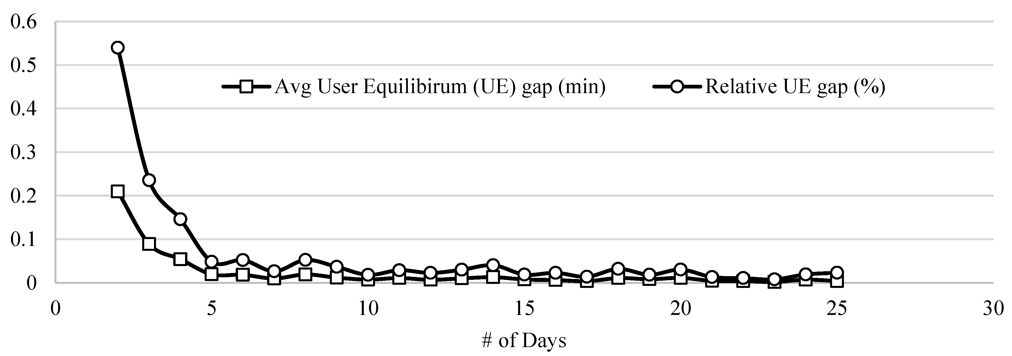
4.7. Dynamic Traffic Simulation

The variability in traffic distribution is a challenging task to predict as it differs based on the regional characteristics, dynamic environmental parameters, and more. DTA aims to predict such changes and variabilities for the long-term behavior of traveler’s adaptation to experienced congestion on the roads. Therefore, the demand distribution or demand profile with congestion periods can vary per each link. The demand profile usually shows two peaks, one in the morning and the other in the afternoon. Such distribution examples can be seen from several sources such as [60,61]. To get a better picture of the demand for a region, we would require long-term data collection of the traffic. This, however, cannot be achieved as the current transportation infrastructure of Cyprus has not yet transitioned to the long-term travel forecasting phase by using traffic counting tools or modeling software. Therefore, to analyze the transportation, certain assumptions based on perceived demand and supply of the region and engineering judgments and intuition were made.
After the collection and the estimation of the necessary information to create a transportation network of our study region, we proceeded to model the DTA in NeXTA DTALite simulation software. To make the task easier, we assigned the necessary attributes (e.g., capacity, speed limit, number of lanes) of the transportation network in ArcGIS. We then used the ‘GIS-Import_Export_Tool’ bundled with the software to make the conversion from the ArcGIS network to the required data format used by the software. It should be noted that NeXTA DTALite input files are in .CSV format, and in order to convert the data to a readable format, we constructed a network dataset of the road network in ArcGIS. This creates the Cost OD Matrix, which in turn outputs the road network in terms of ‘From Node” and “To Node” format. By using the gravity model, we created the OD matrix between the zones and distributed the trips according to the production and attraction of each zone. Without access to the complete data, we cannot produce real values of zonal production and attraction. However, to calibrate and to make traffic volume more realistic, we incorporated AADT for the bridge-links in which the 1 hour peak daily flow was available. We also applied demand multiplication until we observed a realistic volume of traffic.
We distributed the daily traffic demand in the network, as shown in Figure 7. We assumed that peak traffic would happen during 9–10:00 in the morning and 17–18:00 in the evening. We applied a 10-fold increase in the demand to meet the actual volume of traffic in the network. We verified this for the bridge-links according to their designated AADT. We simulated the traffic flow for 25 days–10 days to reach UE and 15 days to optimize the OD Matrix Estimation (ODME)–using known flow volumes of the bridge-links. The traffic was simulated from 9:00 in the morning until 18:00, with a 30 min leeway to smooth the distribution. Figure 8 shows the UE convergence of the simulated network after 25 days. To verify the simulated volumes, we observed the link associated with bridge 6 which has an AADT of about 4317 veh/day and the simulated number of vehicles passing through the link estimated at 4147 veh/day for the whole duration of the simulation.
In summary, 19,110 vehicles were simulated in this analysis, with a total travel time of 5.5 thousand minutes and an average travel time of 29 min between the OD pairs. Some of the results above might be overestimated due to a lack of knowledge on the travel patterns and detailed traffic flow, and the estimated values might not reflect reality. However, such a model can still be used as a baseline to compare with post-event effects for evaluating the performance of the transportation network.

5. Seismic Risk Assessment of Northern Cyprus Transportation Network

The selected region for this research was limited to the western part of Cyprus. It was previously shown that this part of the island can experience earthquake moment magnitudes of up to M7.4. The probability of such events, however, is extremely low. Due the fact that Cyprus has previously encountered devastating historical earthquakes outside our recorded history, e.g., 1222 Cyprus (~M7.0–7.5), the risk of experiencing severe events is high, as these events have return periods of 1000–2500 years. To realize different earthquake scenarios, we used ShakeMap models for the seismic hazards input into HAZUS. We then used the outputs of HAZUS, i.e., the component damage states of bridges for the transportation network and incorporate the results for assessing the vulnerability of the network in terms of different performance indicators described in Section 4.

5.1. Earthquake Scenarios

The choice of the location for simulating different earthquake magnitudes and depths can significantly influence the loss estimation results. Given that the study region is quite large (approx. 50 × 50 km2), for a very strong to a severe event (0.25–0.4 g PGA), the structural loss can vary significantly. Since the bridges are distributed in three different districts, mainly on a stretch of one continuous link, we simulated three different scenarios using ShakeMap with the parameters specified in Section 3.2 and the same scenarios in HAZUS’ arbitrary hazard module. The latter was done for validation purposes. GMPE in HAZUS hazard analysis was only limited to one model, and it was assigned as Boore and Atkinson [29]. The scenarios’ parameter selection is shown in Table 6.
The events listed in the table for the Scenario 1are closely related to a 2475-year return period, Scenarios 2 and 3 fall in the 975-year return period; and finally, Scenario 4 shows an event with a 475-year return period [26]. Seismic events with a 10% probability of exceedance in 50-years (i.e., 475-year return period) resulted in a PGA of around 0.3 g, similar to previous studies. For most bridges, however, such moderate to strong shaking intensities would not result in severe failures. This is more evident for the bridges in Cyprus that are typically short-span and exhibit a high modulus of elasticity. To simulate the worst-case scenario, we, therefore, relied on events that could produce at least 0.40 g PGA. These events would likely fall in the 975-year return period or higher events [26].

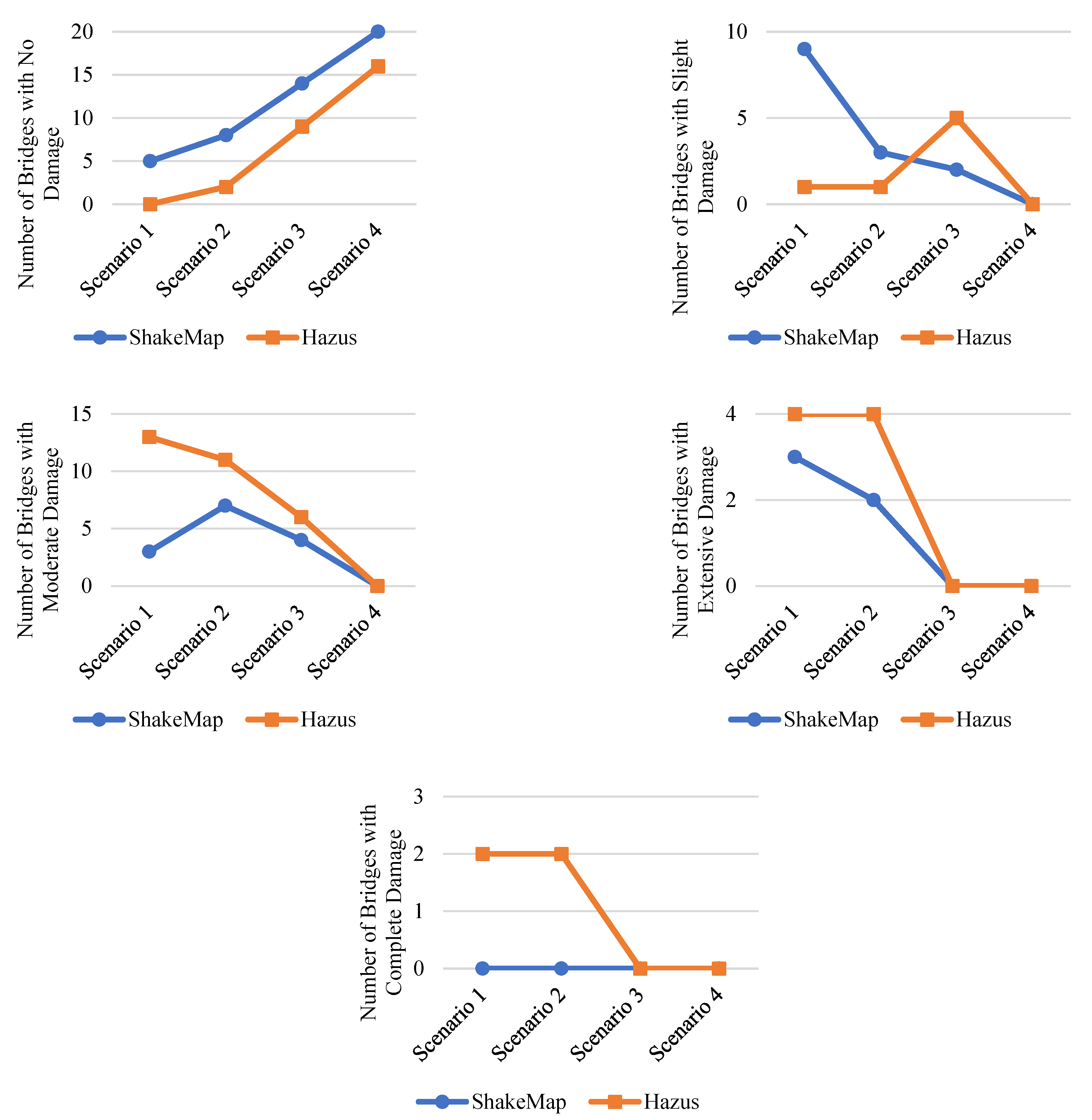
5.2. Structural Loss Estimation from ShakeMap Hazard Maps

From Table 2 for each best damage ratios (from now on, referred to as the mean damage ratio D R d s ) and for each range of D R d s , we can calculate the mean μ m and the standard deviation σ m of damage states for an event m per bridge as:
μ m = k = 1 4 P ( D S = k | I M m ) D R d s k
σ m = k = 1 4 P ( D S = k | I M m ) [ D R d s k μ m ] 2
For these calculations, the “None” damage state is neglected. Table 7 shows the overall damage states for the bridges considering Scenario 1. The overall mean damage state for Scenario 1 is depicted in Figure 9.
We can observe that with an increase in the magnitude of an earthquake event and how close the bridges are to the epicenter, the possibility of the higher damage state. The only exception would be for Scenario 1 where bridges KK000001 and KK000004 experience extensive damage as is expected due to how close they are located from the epicenter, whereas the other bridges in the vicinity experience a slight damage state. These two particular bridges were assigned a HWB8 class (see Table 5), which shows more susceptibility to damage for any given IM. This is more evident by analyzing their fragility curves in Figure 10. As can be seen from the figure, the exceedance probabilities of HWB8 are higher than HWB3. Therefore, for the same level of IM, HWB8 experiences a higher damage state probability.
In general, we can summarize the distribution of damage states for the four bridge classes defined in the region in Table 8.

5.3. Structural Loss Estimation from HAZUS Hazard Module

To validate and compare the structural loss obtained from ShakeMap hazard data, we performed the same analysis in HAZUS built-in hazard module. In the deterministic hazard section of HAZUS, “Arbitrary event” was selected with attenuation function set as Boore and Atkinson Strike-Slip fault type [62]. The fault parameters of the simulated scenarios were based on the fault located on the western coast of Cyprus. Therefore, a fault rupture orientation of 28° CW from N and a 70° dip angle was selected for each of the four scenarios. Surface and subsurface rupture lengths were automatically calculated based on the magnitude using the empirical relationships described in [63].
The comparison between HAZUS and ShakeMap damage estimates is illustrated in Figure 11. In the HAZUS arbitrary event module, the none damage state appears to be lower in number when compared to ShakeMap. This is more noticeable for higher earthquake magnitudes, i.e., Scenario 1 or 2. This means that there are more bridges, for each scenario, that experience at least slight damage. Looking at the graph for slight damage state, one can see that ShakeMap hazard estimates cause more slight damage for higher magnitudes than HAZUS built-in hazard estimates. As the magnitude decreases, however, the reverse is true, at least up to a certain limiting magnitude (in Scenario 4, both methods result in no slight damage). For both moderate and extensive damage states, the HAZUS hazard module produced a higher number of damaged bridges associated with the damage states mentioned above. Therefore, from the first four damage states, we can draw a conclusion in which the ShakeMap hazard approach caused bridges to exhibit none or slight damage. In contrast, there were more damaged bridges related to moderate and extensive damage states in HAZUS. Additionally, we can see complete damage to some bridges in HAZUS hazard estimations, in which there were none for the ShakeMap model.
The apparent differences between the two approaches are probably due to two main reasons: different GMPEs and the assumptions made in ShakeMap that includes no fault/rupture definition. Also, the default fault assignment in HAZUS can contain high degrees of uncertainty. Typically, in the orientation, dip angle, and surface rupture length. This is more significant for high magnitudes of earthquakes. Therefore, the fragility curves in HAZUS with ShakeMap input can only be used as the basis of the structural and operational loss estimation. With the incorporation of the actual fragility curves and adjustment to ShakeMap hazard analysis in the future, we can expect a better representation and estimation of the losses due to seismic events.

5.4. Estimation of Bridge Restoration Model

Depending on the overall level of the damage, we can estimate the direct cost, or more precisely, the restoration cost of the bridges. As explained before, it is assumed that the repair cost is proportional to the replacement value. This relationship was described as damage ratios modified after HAZUS. Using the following equation, we can determine bridge restoration cost C R P m for an event m as:
C R P m = n = 1 N μ m C n
where μ m is the mean damage state per bridge for event m and C n is the replacement cost of bridge n . The replacement cost is calculated by multiplying the deck area by the unit area replacement cost. The replacement cost of the bridges is indicated in Table 9.
The total structural loss for the four scenarios is shown in Figure 12. As can be observed from the figure, Scenario 2 incurred higher structural loss compared to a higher magnitude scenario (e.g., Scenario 1, M7.4 event) because there were more vulnerable bridges in the region. Moreover, HWB8 generated higher losses as expected. The exceedance probabilities of this class of bridges are higher, as previously described. The uncertainties in the derivation of the losses can vastly impact the strategy taken to mitigate such losses.
For mitigation scenarios, where retrofit strategy is applied for certain bridges, the retrofit cost C R can be expressed as being proportional to the replacement value as:
C R m = m = 1 M C R P m r m
where r n is the retrofit cost ratio set equal to 20%. This is independent of the seismic event, and due to the complexity of the estimating retrofit value for each bridge, the ratio is assumed to be constant. Seismic retrofitting of bridges before earthquake events, assuming that it does not exceed the total repair cost of the bridge, can reduce the structural losses significantly. The reduction in the loss can be assigned as the benefit achieved from avoiding replacement costs. In the subsequent section, the cost-effectiveness of bridge retrofit, including the operational losses in terms of cost-benefit analysis, was investigated.
The amount of time required to repair a damaged bridge depends on the state of the damage. The HAZUS methodology assumes the bridge capacity starts to recover right after the event and increases following a CDF function. The HAZUS CDF restoration model is expressed as:
R ( t ) = Φ ( t m t , d s σ t , d s )
where m t , d and σ t , d indicate mean and standard deviation of the restoration curve parameters for each of the damage state d s . HAZUS provides the necessary parameters for developing restoration curves for each damage state, as shown in Table 10.

5.5. Post-Earthquake Network Reliability Indices

For the scenarios tested in this study, the bridge network did not suffer from complete failure. To determine the post-earthquake network topological indicators, however, we need to assume temporary network failure for certain bridges. Therefore, based on restoration curves generated before, we assumed for the first couple of days after an earthquake, bridges that experienced moderate to complete damages are non-functional. Therefore, for each scenario, these bridges and the links associated with these bridges were removed from the network. The results of the topological vulnerability analysis are shown in Table 11. In terms of reliability, Scenario 2 is the worst-case scenario. On average, however, the first three scenarios have shown a reduction in the network reliability indices. There was no change in Scenario 4 as expected.

5.6. Post-Earthquake Structural Loss at Node and Edge Level

Table 12 presents the results of the transportation network structural loss for the scenarios simulated in this study. Like Table 11, we can observe that Scenario 2 showed, on average, the maximum amount of network structural loss. The results above suggest that the district of Guzelyurt (Scenario 2) is more vulnerable to losses in the transportation network in terms of the indicators explained previously.
Following the outcomes in the direct loss estimation, the district of Guzelyurt, is in fact, in the risk of catastrophic failure. Scenario 2 was proven to be the worst outcome that can potentially result in total isolation of the district from the nearby districts, cities, and villages. To demonstrate this risk visually, in the case of similar events as in Scenario 2, we can expect a damaged transportation network, as shown in Figure 13. The outcome of this scenario is devastating as it will completely cut off fast access to nearby cities and villages for the first responders. To mitigate the catastrophic situations, there needs to be a policy change. Firstly, retrofitting of the vulnerable bridges in an optimal manner. Some bridges are already deteriorating due to weather, flood, and other hazards in the region. The analysis of this study does not consider deterioration effects; therefore, even the bridges that are undamaged or slightly damaged could be at serious risk of total collapse, even for smaller earthquake magnitudes. Secondly, mitigation strategies have to be put in place to accommodate emergency responders as fast as possible in a case of network failure. This can be done by providing detour roads around vulnerable links. Doing so will keep the functionality of the network at a reasonable level.

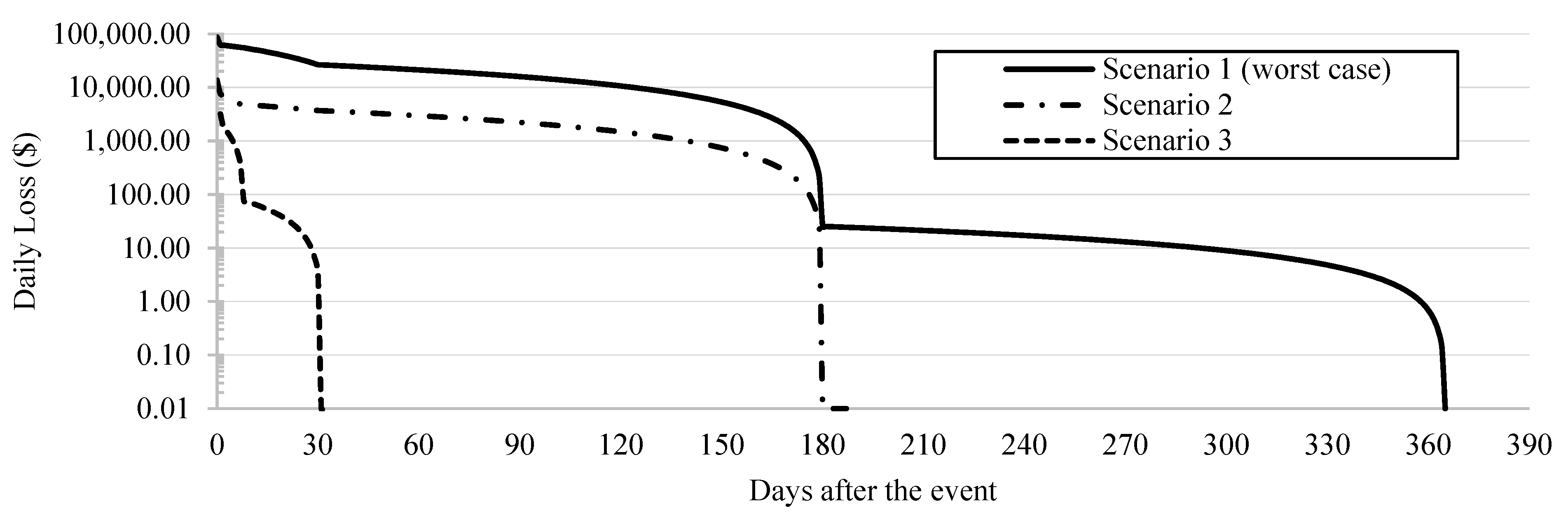
5.7. Travel Time Loss Estimation

To simulate the travel time loss of the transportation network, some assumptions have been made. We suppose that the post-event demand is the same as the pre-event to consider the worst-case. One reason is that robust and reliable OD reduction factors are hard to calculate and are not universal. Socio-economic characteristics and the culture of the region also play essential roles in determining OD changes. The second assumption is related to the reduction of road capacities. Nevertheless, several works have attempted to quantify traffic post events using resiliency and reliability methods [64,65]. A transportation network is designed in such a way that, detouring traffic through alternative roads can be possible in cases when one or more links become inaccessible in a network for some reason. Hence, all links can have residual capacities for each damage state that can accommodate a certain percent of traffic flowing in the network. Therefore, depending on the damage degree, the nominal capacities of the roads, as well as the free-flow speed, will be reduced by a residual percentage. We adopted the methodologies described in [11] and [10] for a moderate residual link traffic carrying capacity and free-flow speed reduction, respectively, as shown in Table 13.
DTALite was used with the same parameters to simulate day 0 (i.e., immediately after an earthquake). The results are presented in Table 14. Here, Scenario 1 is the worst-case event in terms of total travel time loss.
The travel time loss in terms of monetary values, i.e., operational cost, can be calculated as the product of the vehicle car occupancy (VCO), the value of time, and total travel time loss. OD demand is given in passenger car units. To estimate the number of passengers traveling in a single car, an average occupancy factor is needed. We used VCO = 1.50 based on parameters presented in [66]. The value of time is based on the socio-economic profile of the region. Such studies have not been done before for Cyprus. Therefore, we assumed 17 $/h on average as the value of time. To estimate the total loss over time, we performed the same analysis for each scenario for 1, 7, 30, 180, and 365 days after the event has occurred. The recovery of the bridge functionality and its corresponding links follow the curve restoration curves. The discrete value of percent-restoration is found for each damage state. Assuming a linear decrease of the daily loss between the days as mentioned above, we can construct a plot showing the operational daily loss overtime for the first three scenarios. Hence, the total operational loss for each scenario is computed by integrating the curves in Figure 14 (there is no operational loss in Scenario 4).
From the figure, we can observe that Scenario 1 produces the largest operational loss until all the bridges in the network return to 100% functionality, which could take up to a year. This results in a total indirect cost of $3,439,478. Scenarios 2 and 3 result in $433,296 and $10,481, respectively. The operational loss well exceeds the structural loss for each scenario. This is particularly important as it is often ignored by the relevant authorities. Although, it should be noted that we assumed a fixed demand case, which sometimes does not reflect the reality for some regions. The study in [8] showed that variable travel demand could decrease the total travel time loss by almost a factor of 10−4, which is quite small. Moreover, the traffic analysis in this study only considered commuter traffic delays. The value of time of truck drivers and the value of the cargo can sometimes be five or six-fold more than that of public commuters [8,66].

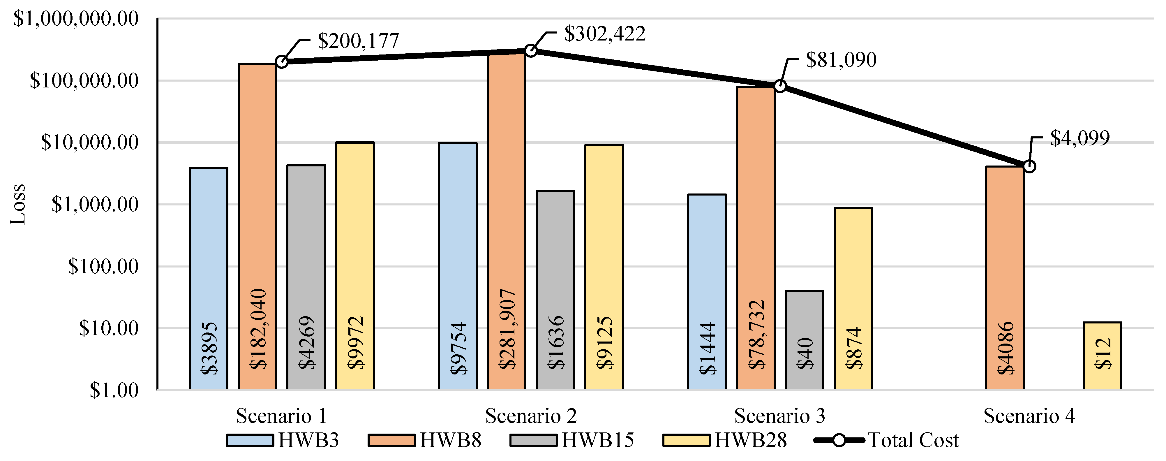
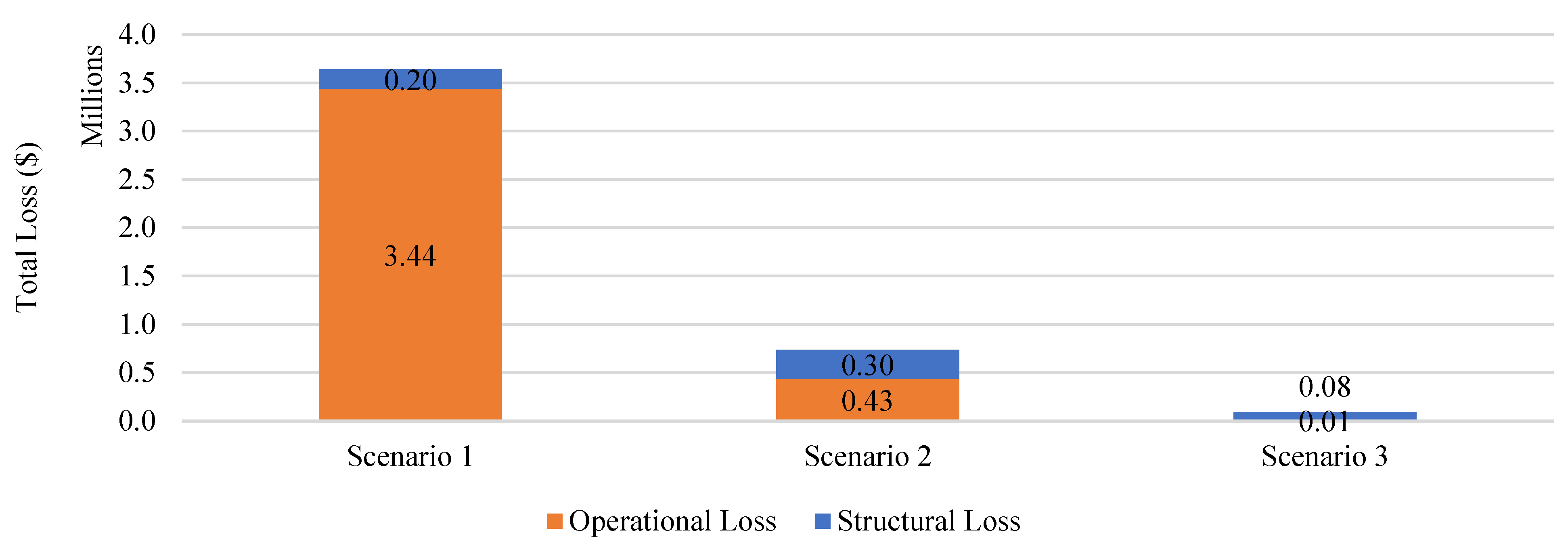
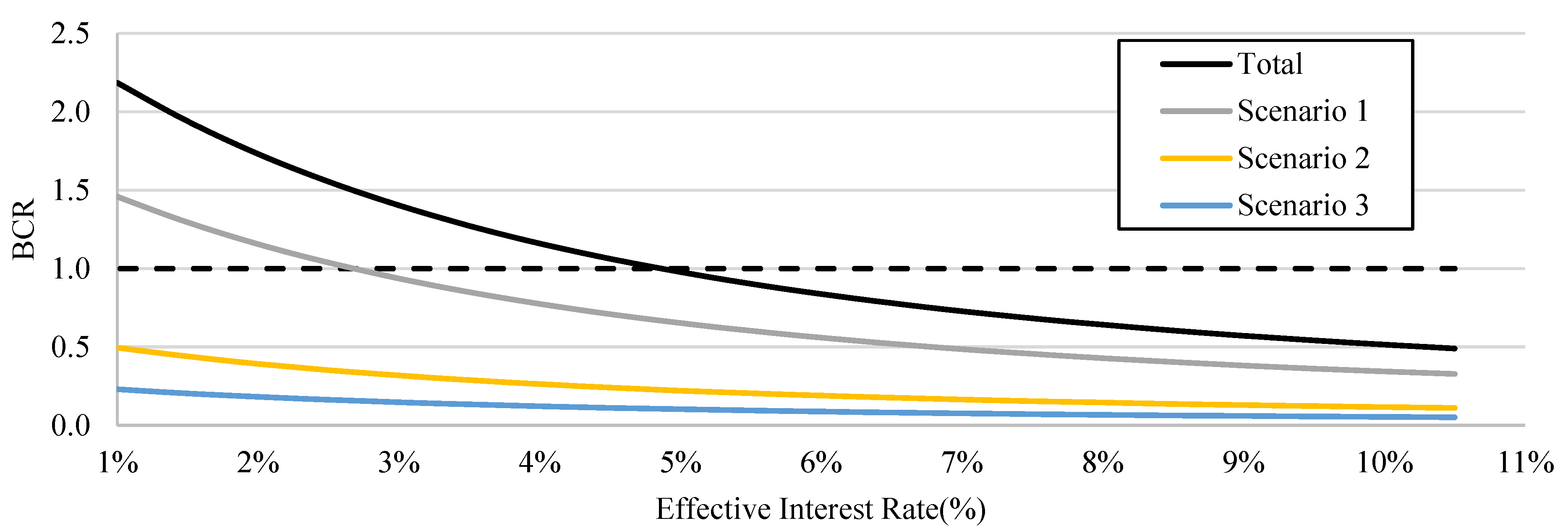
5.8. Operational and Structural Loss Aggregation, Economic Analysis of Bridge Retrofitting

Before any mitigation strategies such as seismic bridge retrofit, the total operational and structural losses were summed to estimate the total seismic loss for each event. The operational loss is the crucial changing factor in determining the best policy to be implemented to reduce the overall losses incurred by a region. Although, given the limited number of bridges in the study region, and the uncertainties in the damage state bridges experience, we still believe that indirect costs are significant and should not be ignored. The aggregated losses for three different scenarios are shown in Figure 15 (the total loss in Scenario 4 is almost zero; therefore, it is not shown in the figure).
After applying the seismic retrofitting of bridges before the event, we expected to have reductions in the total seismic loss, including the structural and the operational losses. This reduction was considered as the benefit achieved by avoiding these losses. The model below is presented in [67] and slightly modified to fit our analysis. Hence, the cost avoided for the repair/restoration cost for an event m can be modeled as:
B ¯ S L m = C R P m 0 C R P m R
where B ¯ S L m is the expected benefit from costs avoided from structural loss; C R P m 0 , and C R P m R are the system restoration cost with and without retrofitting. Since detailed computational work is required to find new damage state probabilities of the retrofitted bridges, for simplicity, we assumed that retrofitting would ensure 90% cost saving for both the structural and operational losses, i.e., C R P m R = 0.10 × C R P m 0 .
Similarly, the expected annual benefit from the avoided operational loss for an event m B ¯ O L m is expressed as:
B ¯ O L m = C O L m 0 C O L m R
where, C O L m R , and C O L m o are the operational losses with and without retrofitting, respectively. Therefore, the annual benefit from retrofitting is calculated by adding the costs avoided in structural and operational losses as:
B ¯ = m = 1 M [ B ¯ O L m + B ¯ S L m ] p m
where B ¯ is the annual benefit and p m is the annual probability of event m , or simply its annual recurrence rate. To compute the total benefit over the residual service life T , and assuming uniformly distributed annual benefit through the period, the total present value of the benefit B P V for an effective interest rate r for a time period T is expressed as:
B ¯ P V = t = 1 T B ¯ ( 1 + r ) t = B ¯   ( 1 + r ) T 1 r ( 1 + r ) T
The effective interest rate r is not easy to calculate, therefore, to show the effect of different interest rates assuming T = 50 years, the total benefit-cost ratio B C R = m M B P V m / C R m for a range of rates is shown in Figure 16. According to the figure, we can observe that for the study region until 4.25% discount rate, the retrofitting strategy is cost-effective. Seismic loss analysis is susceptible to bridge damage state and link residual capacities, in addition to the restoration functions. Therefore, future studies should incorporate the sensitivity analysis of the parameters assumed here. Moreover, the transportation network in this study only considered the main roadway links in the region. Local detour link analysis should be integrated into the analysis to determine the best possible alternative routes to reduce the residual capacities on the main links. Some of the bridges in Cyprus are historical and date back more than 50 years. Therefore, the service life of bridges will impact the analysis. Lower discount rates and higher bridge service life are more cost-effective. Finally, many of the bridges are already deteriorated, therefore, their capacity to withstand seismic loads are less. This study considered the nominal performance of each bridge, i.e., bridges are at their full capacity while performing seismic assessment. This leads to a more conservative loss estimation model and obscures the real loss incurred on a region; operational losses would be even more prominent.
Bridge seismic retrofit prioritization is a way to determine the most critical bridges in the network. Optimization algorithms based on network simplex models (e.g., minimum cost flow analysis) or maximum flow are typically solved as a mixed-integer linear program. The algorithms under a constraint retrofitting budget can find the most critical links and bridges. This allows the decision-makers to retrofit the most critical components only. Bridge retrofit prioritization is out of the scope of this study. As a general framework, therefore, bridge retrofit prioritization should be integrated with local detours and linked directly to seismic loss tools or analytical loss models with sensitivity assessments to calibrate for the best parameters to find the expected seismic loss and benefit for a region.

6. General Remarks and Limitations

This study aimed to perform a seismic risk assessment of Cyprus and lay the initial foundations to develop a risk-informed decision-making system. Using modern tools and methodologies, the analysis of the seismic hazards and the transportation network in this study enabled us to determine the best strategies reducing the overall losses for the scenarios tested here. The following provides a general overview of our findings and conclusions for the objectives of this study. The present research can provide useful information and data to the responsible agencies in the hope that the results of this study can be used to reduce the risk of earthquakes in the future. With improvements in this study and conducting assessment of the whole island, we believe Cyprus can be better prepared for potential hazards in the future. Therefore, we suggest the following proactive measures assembled from the findings of our study:
  • Developing a real-time seismic hazard and risk assessment.
  • Initiating a localized hazard assessment of the critical regions. e.g., district of Lefke.
  • Gathering a comprehensive transportation network data, including the road characteristics, travel time estimation and socioeconomic parameters taken from detailed surveys.
  • Retrofitting vulnerable links and bridges as identified in this study.
  • Providing detour links in the areas where the risk of bridge failure is high, especially in the district of Lefke where no detour links exist.
This study cannot represent accurate losses incurred by the region following an earthquake event in full detail and some limitations and assumptions were inevitable.
ShakeMap data and the HAZUS built-in hazard module do not include the fault information of the region. Therefore, the hazard maps generated for the three different scenarios in ShakeMap and HAZUS are slightly overestimated. Moreover, the fragility curves assumed for the bridges in the study region follow the default HAZUS fragility function. The damage functions are aggregated in 28 highway bridge classes defined in HAZUS for U.S. bridges. This can result in an underestimation or overestimation of some bridges’ damage state functions for a given IM. Therefore, to represent the actual fragility curves, a detailed analysis is required. However, initial steps to achieve this was made in a parallel research study by the authors in [68].
The vulnerability parameters only considered the network as a whole and ignored some essential components in urbanization, such as the evolution over time in hazard exposure and community vulnerability exposure. As urbanization increases, the model complexity increases at the same rate. This results in the degradation of the network over time. Therefore, time-dependent factors should be incorporated into future studies. In terms of the link performance measure, some significant portion of this section had to be assumed as data availability was either limited or non-existent. Data such as the actual demand of the network, the road network capacity, and the traffic need to be updated for a more realistic analysis in the future.
The simulation and parameters used in the analysis are uncertain. The earthquake scenarios evaluated are limited in number and variety. The spatial correlation in ground shaking of these scenarios is another factor that can significantly influence the hazard modeling of the study. Moreover, the cost variables in cost estimation of the structural loss and operational loss are assumed for the region. Future studies are, therefore, required to calibrate these values through sensitivity analysis. Furthermore, one significant aspect of suggesting cost-effective mitigations strategies is to develop bridge retrofit prioritization models. In this way, under a constraint budget, we can retrofit those bridges which are vital in keeping the transportation network at a reasonably functional level.

7. Future Work and Conclusions

Under the umbrella of a synergistic combination of an intelligent structural health motoring (SHM) and GIS cloud-based bridge monitoring system, we believe the system architecture presented as shown in Figure 17, is cost-effective, efficient, and sustainable solution in bridge prognosis and diagnosis. The capability of this system can be further enhanced by utilizing machine learning techniques [69,70]. This system can also be linked to an ITS platform for better integration into a smart city paradigm under SHM-informed-ITS models. The new paradigm shift in the incorporation of new and innovative technologies for bridge seismic risk assessment can offer many prospects in this field. Notably, we can expect to see a real-time bridge assessment immediately after an event. In case of damage or total collapse of a bridge, in order to keep the performance of the transportation network at high levels to ensure a fast emergency response to reduce other the social costs, ITS can come into play to suggest alternative routes or provide real-time traffic information to reduce operational costs. The opportunities in this field are vast, and as time goes by, with the increase in complexity of the transportation network, the need to change to a better decision-making system becomes more critical. The methods and concepts described in this study can be considered as the next step toward the future of the cyber-physical system (CPS) as part of the Internet of Things (IoT) paradigm shift. The future of the risk assessment of a transportation network lies within the smart city and cloud technology.
The risk assessment of bridges applied to a case study of Cyprus is the first of its kind for the region and also equally important in terms of the seismic risk reduction findings in the country. The results of this study can provide responsible agencies with a framework that can visualize different scenarios, and consequently apply the best mitigation strategies to minimize the overall losses. Analyzing network vulnerability and reliability can provide an in-depth understanding of the current and future impacts of seismic risks associated with highway-bridge networks. The three factors of sustainability (i.e., economic, social, and environmental) considering the resiliency of the transportation network following a seismic event can significantly influence the decisions taken in mitigation, planning, response, and recovery stages. Therefore, hazard-induced sustainability metrics have to be integrated into the risk assessment studies and planned in the initial design stage of the bridge transportation network. While this study focused on seismic risks, the major hazard that Cyprus is usually faced with is flooding. In that sense, the general framework, models, and software used in this study can be easily extended to other hazard analyses. Thereby, the losses due to floods can also be included in the analysis to provide an all-in-one multi-hazards assessment tool.

Author Contributions

Conceptualization, A.M. and E.O.; methodology, A.M.; software, A.M.; validation, A.M., E.O. and W.R.; formal analysis, A.M.; investigation, A.M., E.O. and W.R.; resources, A.M., E.O. and W.R.; data curation, A.M. and W.R.; writing—original draft preparation, A.M.; writing—review and editing, A.M., E.O. and W.R.; visualization, A.M.; supervision, E.O.; project administration, E.O.; funding acquisition, E.O. All authors have read and agreed to the published version of the manuscript.

Funding

This research received no external funding.

Data Availability Statement

All data that support the findings of this study are available from the corresponding author upon reasonable request. Additionally, all data used during this study appear in the submitted article.

Conflicts of Interest

The authors declare no conflict of interest.

References

  1. Little, R.G. Controlling Cascading Failure: Understanding the Vulnerabilities of Interconnected Infrastructures. J. Urban Technol. 2002, 9, 109–123. [Google Scholar] [CrossRef]
  2. Basöz, N.; Kiremidjian, A.S. Risk Assessment for Highway Transportation Systems. John, A.B., Ed.; Earthquake Engineering Center Technical Report 118, USA. 1996. Available online: http://purl.stanford.edu/fr998kq2251 (accessed on 27 July 2020).
  3. Tomaszewski, B. Geographic Information Systems (GIS) for Disaster Management, 1st ed.; Routledge: Boca Raton, FL, USA, 2014. [Google Scholar]
  4. Cheng, M.-Y.; Wu, Y.-W.; Chen, S.-J.; Weng, M.-C. Economic evaluation model for post-earthquake bridge repair/rehabilitation: Taiwan case studies. Autom. Constr. 2009, 18, 204–218. [Google Scholar] [CrossRef]
  5. Enke, D.L.; Tirasirichai, C.; Luna, R. Estimation of Earthquake Loss due to Bridge Damage in the St. Louis Metropolitan Area. II: Indirect Losses. Nat. Hazards Rev. 2008, 9, 12–19. [Google Scholar] [CrossRef]
  6. Shi, W.; Cheng, P.G.; Ko, J.M.; Liu, C. GIS-based bridge structural health monitoring and management system. In Proceedings of the Nondestructive Evaluation and Health Monitoring of Aerospace Materials and Civil Infrastructures, San Diego, CA, USA, 18 June 2002; Volume 4704, pp. 12–19. [Google Scholar] [CrossRef]
  7. Chiu, Y.C.; Bottom, J.; Mahut, M.; Paz, A.; Balakrishna, R.; Waller, S.; Hicks, J. Dynamic Traffic Assignment: A Primer; Transportation Research Board: Washington, DC, USA, 2011; Available online: https://onlinepubs.trb.org/onlinepubs/circulars/ec153.pdf (accessed on 19 July 2020).
  8. Kiremidjian, A.; Moore, J.; Fan, Y.Y.; Yazlali, O.; Basoz, N.; Williams, M. Seismic Risk Assessment of Transportation Network Systems. J. Earthq. Eng. 2007, 11, 371–382. [Google Scholar] [CrossRef]
  9. Barbat, A.H.; Carreño, M.L.; Pujades, L.G.; Lantada, N.; Cardona, O.D.; Marulanda, M.C. Seismic vulnerability and risk evaluation methods for urban areas. A review with application to a pilot area. Struct. Infrastruct. Eng. 2010, 6, 17–38. [Google Scholar] [CrossRef]
  10. Guo, A.; Liu, Z.; Li, S.; Li, H. Seismic performance assessment of highway bridge networks considering post-disaster traffic demand of a transportation system in emergency conditions. Struct. Infrastruct. Eng. 2017, 13, 1523–1537. [Google Scholar] [CrossRef]
  11. Zhou, Y.; Banerjee, S.; Shinozuka, M. Socio-economic effect of seismic retrofit of bridges for highway transportation networks: A pilot study. Struct. Infrastruct. Eng. 2010, 6, 145–157. [Google Scholar] [CrossRef]
  12. Kilanitis, I.; Sextos, A. Integrated seismic risk and resilience assessment of roadway networks in earthquake prone areas. Bull. Earthq. Eng. 2019, 17, 181–210. [Google Scholar] [CrossRef] [Green Version]
  13. Padgett, J.E.; Desroches, R.; Nilsson, E. Regional Seismic Risk Assessment of Bridge Network in Charleston, South Carolina. J. Earthq. Eng. 2010, 14, 918–933. [Google Scholar] [CrossRef]
  14. Chang, L.; Elnashai, A.S.; Spencer, B.F. Post-earthquake modelling of transportation networks. Struct. Infrastruct. Eng. 2012, 8, 893–911. [Google Scholar] [CrossRef]
  15. Luna, R.; Hoffman, D.; Lawrence, W.T. Estimation of Earthquake Loss due to Bridge Damage in the St. Louis Metropolitan Area. I: Direct Losses. Natural Hazards Review; American Society of Civil Engineers (ASCE): Reston, VA, USA, 2008; Volume 9, pp. 1–11. [Google Scholar] [CrossRef]
  16. Stergiou, E.C.; Kiremidjian, A.S. Risk assessment of transportation systems with network functionality losses. Struct. Infrastruct. Eng. 2010, 6, 111–125. [Google Scholar] [CrossRef]
  17. Shinozuka, M.; Murachi, Y.; Dong, X.; Zhou, Y.; Orlikowski, M.J. Effect of seismic retrofit of bridges on transportation networks. Earthq. Eng. Eng. Vib. 2003, 2, 169–179. [Google Scholar] [CrossRef] [Green Version]
  18. Codermatz, R.; Nicolich, R.; Slejko, D. Seismic risk assessments and GIS technology: Applications to infrastructures in the Friuli-Venezia Giulia region (NE Italy). Earthq. Eng. Struct. Dyn. 2003, 32, 1677–1690. [Google Scholar] [CrossRef]
  19. Rozelle, J.R. International Adaptation of the Hazus Earthquake Model Using Global Exposure Datasets. Master’s Thesis, University of Colorado, Denver, CO, USA, 2018. Available online: https://search.proquest.com/docview/2138380714/abstract/19F245120FBC497FPQ/1 (accessed on 22 June 2020).
  20. McGrath, H.; Stefanakis, E.; Nastev, M. Sensitivity analysis of flood damage estimates: A case study in Fredericton, New Brunswick. Int. J. Disaster Risk Reduct. 2015, 14, 379–387. [Google Scholar] [CrossRef]
  21. Fallah-Aliabadi, S.; Ostadtaghizadeh, A.; Ardalan, A.; Eskandari, M.; Fatemi, F.; Mirjalili, M.R.; Khazai, B. Risk analysis of hospitals using GIS and HAZUS: A case study of Yazd County, Iran. Int. J. Disaster Risk Reduct. 2020, 47, 101552. [Google Scholar] [CrossRef]
  22. Silva, V.; Crowley, H.; Pagani, M.; Monelli, D.; Pinho, R. Development of the OpenQuake engine, the Global Earthquake Model’s open-source software for seismic risk assessment. Nat. Hazards 2013, 72, 1409–1427. [Google Scholar] [CrossRef]
  23. Cagnan, Z.; Tanircan, G.B. Seismic hazard assessment for Cyprus. J. Seism. 2009, 14, 225–246. [Google Scholar] [CrossRef]
  24. Jena, R.; Pradhan, B.; Beydoun, G.; Al-Amri, A.; Sofyan, H. Seismic hazard and risk assessment: A review of state-of-the-art traditional and GIS models. Arab. J. Geosci. 2020, 13, 50. [Google Scholar] [CrossRef]
  25. Geological Survey Department Cyprus. Cyprus Broadband Seismological Network [Data set]. International Federation of Digital Seismograph Networks. 2013. Available online: https://www.fdsn.org/networks/detail/CQ/ (accessed on 1 August 2022). [CrossRef]
  26. Woessner, J.; Laurentiu, D.; Giardini, D.; Crowley, H.; Cotton, F.; Grünthal, G.; Valensise, G.; Arvidsson, R.; Basili, R.; Demircioglu, M.B.; et al. The 2013 European Seismic Hazard Model: Key components and results. Bull. Earthq. Eng. 2015, 13, 3553–3596. [Google Scholar] [CrossRef] [Green Version]
  27. Gross, J.L.; Phan, L.T. Implications for Earthquake Risk Reduction in the United States From the Kocaeli, Turkey, Earthquake of August 17, 1999. In ASCE World Structural Engineering Conference (USGS Circular 1193); USA; 2000; Volume 1193. Available online: https://www.nist.gov/publications/implications-earthquake-risk-reduction-united-states-kocaeli-turkey-earthquake-august (accessed on 14 July 2020).
  28. Barka, A.; Reilinger, R. Active tectonics of the Eastern Mediterranean region: Deduced from GPS, neotectonic and seismicity data. Ann. Geophys. 1997, 40, 2. [Google Scholar] [CrossRef]
  29. Boore, D.M.; Atkinson, G.M. Ground-Motion Prediction Equations for the Average Horizontal Component of PGA, PGV, and 5%-Damped PSA at Spectral Periods between 0.01s and 10.0s. Earthq. Spectra 2008, 24, 99–138. [Google Scholar] [CrossRef] [Green Version]
  30. Campbell, K.W.; Bozorgnia, Y. NGA-West2 Ground Motion Model for the Average Horizontal Components of PGA, PGV, and 5% Damped Linear Acceleration Response Spectra. Earthq. Spectra 2014, 30, 1087–1115. [Google Scholar] [CrossRef]
  31. Akkar, S.; Bommer, J.J. Empirical Equations for the Prediction of PGA, PGV, and Spectral Accelerations in Europe, the Mediterranean Region, and the Middle East. Seism. Res. Lett. 2010, 81, 195–206. [Google Scholar] [CrossRef] [Green Version]
  32. Cagnan, Z.; Yilmaz, O.; Yilmaz, T. Site Classification of Newly Deployed Strong Motion Stations in the Eastern Mediterranean. Presented at the 15th World Conference on Earthquake Engineering, Lisbon, Portugal, 24 September 2012. [Google Scholar]
  33. Nielson, B.G. Analytical Fragility Curves for Highway Bridges in Moderate Seismic Zones. Ph.D. Thesis, Georgia Institute of Technology, Atlanta, GA, USA, 2005. [Google Scholar]
  34. NIBS-FEMA. Hazus®–MH 2.1 Multi-Hazard Loss Estimation Methodology Technical Manual; Department of Homeland Security Federal Emergency Management Agency Mitigation Division: Washington, DC, USA, 2013. [Google Scholar]
  35. Mander, J.B.; Basöz, N. Seismic Fragility Curve Theory for Highway Bridges. In Optimizing Post-Earthquake Lifeline System Reliability; Seattle, WA, USA; 1999; pp. 31–40. Available online: https://cedb.asce.org/CEDBsearch/record.jsp?dockey=0118440 (accessed on 2 May 2019).
  36. Taylor, M.A.P.; D’Este, G.M. Transport Network Vulnerability: A Method for Diagnosis of Critical Locations in Transport Infrastructure Systems. In Critical Infrastructure: Reliability and Vulnerability; Murray, A.T., Grubesic, T.H., Eds.; Springer: Berlin/Heidelberg, Germany, 2007; pp. 9–30. [Google Scholar] [CrossRef]
  37. Bell, M.G.H.; Iida, Y. Transportation Network Analysis; Chichester; John Wiley & Sons: New York, NY, USA, 1997. [Google Scholar]
  38. Rodrigue, J.-P.; Comtois, C.; Slack, B. The geography of Transport Systems, 4th ed.; Routledge: London, UK; Taylor & Francis Group: New York, NY, USA, 2017. [Google Scholar]
  39. Gross, J.L.; Yellen, J.; Zhang, P. (Eds.) Handbook of Graph Theory, 2nd ed.; CRC Press, Taylor & Francis Group: Boca Raton, FL, USA, 2014. [Google Scholar]
  40. Kansky, K.; Danscoine, P. Measures of network structure. FLUX Cah. Sci. Int. Réseaux Territ. 1989, 5, 89–121. [Google Scholar] [CrossRef]
  41. Kansky, K.J. Structure of Transportation Networks: Relationships Between Network Geometry and Regional Characteristics; University of Chicago: Chicago, IL, USA, 1963. [Google Scholar]
  42. Mattsson, L.-G.; Jenelius, E. Vulnerability and resilience of transport systems—A discussion of recent research. Transp. Res. Part A Policy Pract. 2015, 81, 16–34. [Google Scholar] [CrossRef]
  43. Sevtsuk, A.; Mekonnen, M. Urban Network Analysis: A New Toolbox for Measuring City Form in ArcGIS. In Proceedings of the 2012 Symposium on Simulation for Architecture and Urban Design, San Diego, CA, USA, 26–30 March 2012. [Google Scholar]
  44. Okabe, A.; Okunuki, K. A Spatial Analysis along Networks, Version 4.1; SANET: Tokyo, Japa, 2017. [Google Scholar]
  45. Hagberg, A.; Swart, P.; Chult, D.S. Exploring Network Structure, Dynamics, and Function Using Networkx. In Proceedings of the SCIPY 08, Pasadena, CA, USA, 21 August 2008; Los Alamos National Lab. (LANL), Los Alamos, NM (United States), LA-UR-08-05495; LA-UR-08-5495. Available online: https://www.osti.gov/biblio/960616-exploring-network-structure-dynamics-function-using-networkx (accessed on 3 July 2020).
  46. Freeman, L.C. Centrality in social networks conceptual clarification. Soc. Netw. 1978, 1, 215–239. [Google Scholar] [CrossRef] [Green Version]
  47. Sevtsuk, A.; Mekonnen, M.; Kalvo, R. Urban Network AnalysisToolbox for ArcGIS 10/10.1/10.2 Help Manual V1.01; City Form Lab: Seattle, WA, USA, 2016. [Google Scholar]
  48. Handy, S.L.; A Niemeier, D. Measuring Accessibility: An Exploration of Issues and Alternatives. Environ. Plan. A: Econ. Space 1997, 29, 1175–1194. [Google Scholar] [CrossRef]
  49. Okabe, A.; Sugihara, K. Spatial Analysis along Networks: Statistical and Computational Methods; Wiley: Hoboken, NJ, USA, 2012. [Google Scholar]
  50. Okabe, A.; Satoh, T.; Sugihara, K. A kernel density estimation method for networks, its computational method and a GIS-based tool. Int. J. Geogr. Inf. Sci. 2009, 23, 7–32. [Google Scholar] [CrossRef]
  51. Benedek, J.; Ciobanu, S.M.; Man, T.-C. Hotspots and social background of urban traffic crashes: A case study in Cluj-Napoca (Romania). Accid. Anal. Prev. 2016, 87, 117–126. [Google Scholar] [CrossRef]
  52. Xie, Z.; Yan, J. Kernel Density Estimation of traffic accidents in a network space. Comput. Environ. Urban Syst. 2008, 32, 396–406. [Google Scholar] [CrossRef] [Green Version]
  53. U. B. of P. R. O. of P. U. P. Division. Traffic Assignment Manual for Application with a Large, High Speed Computer; US Department of Commerce: Washington, DC, USA, 1964. [Google Scholar]
  54. Duthie, J.C.; Nezamuddin, N.; Juri, N.R.; Rambha, T.; Melson, C.; Pool, C.M.; Boyles, S.; Waller, S.T.; Kumar, R. Investigating Regional Dynamic Traffic Assignment Modeling for Improved Bottleneck Analysis: Final Report; Technical Report FHWA/TX-13/0-6657-1; Center for Transportation Research, University of Texas: Austin, TX, USA, 2013. [Google Scholar]
  55. Tian, Z.; Lin, D.; Yin, K.; Zhou, X. Development of a Dynamic Traffic Assignment Model for Northern Nevada; NDOT Research Report 342-13–803; Center for Advanced Transportation Education and Research (CATER), University of Nevada: Reno, NV, USA, 2014. [Google Scholar]
  56. Zhou, X.; Taylor, J. DTALite: A queue-based mesoscopic traffic simulator for fast model evaluation and calibration. Cogent Eng. 2014, 1, 961345. [Google Scholar] [CrossRef]
  57. Lu, C.-C.; Mahmassani, H.S.; Zhou, X. Equivalent gap function-based reformulation and solution algorithm for the dynamic user equilibrium problem. Transp. Res. Part B Methodol. 2009, 43, 345–364. [Google Scholar] [CrossRef]
  58. Transportation Research Board, Highway Capacity Manual. A Guide for Multimodal Mobility Analysis, 6th ed.; Transportation Research Board: Washington, DC, USA, 2016. [Google Scholar]
  59. Dowling, R.G.; United States, American Association of State Highway and Transportation Officials, National Research Council (U.S.); National Cooperative Highway Research Program (Eds.) Planning Techniques to Estimate Speeds and Service Volumes for Planning Applications; Transportation Research Board, National Research Council: Washington, DC, USA; National Academy Press: Washington, DC, USA, 1997. [Google Scholar]
  60. Sloboden, J.; Lewis, J.; Alexiadis, V.; Chiu, Y.-C.; Nava, E. Traffic Analysis Toolbox Volume Xiv: Guidebook on the Utilization of Dynamic Traffic Assignment in Modeling; Federal Highway Administration. Office of Operations: Washington, DC, USA, 2012. [Google Scholar]
  61. Järv, O.; Ahas, R.; Saluveer, E.; Derudder, B.; Witlox, F. Mobile Phones in a Traffic Flow: A Geographical Perspective to Evening Rush Hour Traffic Analysis Using Call Detail Records. PLoS ONE 2012, 7, e49171. [Google Scholar] [CrossRef] [PubMed] [Green Version]
  62. Cornell, C.A.; Banon, H.; Shakal, A.F. Seismic motion and response prediction alternatives. Earthq. Eng. Struct. Dyn. 1979, 7, 295–315. [Google Scholar] [CrossRef]
  63. Wells, D.L.; Coppersmith, K.J. New empirical relationships among magnitude, rupture length, rupture width, rupture area, and surface displacement. Bull. Seismol. Soc. Am. 1994, 84, 974–1002. [Google Scholar]
  64. Ghasemi, S.H.; Lee, J.Y. Measuring Instantaneous Resilience of a Highway Bridge Subjected to Earthquake Events. Transp. Res. Rec. J. Transp. Res. Board 2021, 2675, 1681–1692. [Google Scholar] [CrossRef]
  65. Ghasemi, S.H.; Lee, J.Y. Reliability-based indicator for post-earthquake traffic flow capacity of a highway bridge. Struct. Saf. 2020, 89, 102039. [Google Scholar] [CrossRef]
  66. Dong, Y.; Frangopol, D.M.; Saydam, D. Sustainability of Highway Bridge Networks Under Seismic Hazard. J. Earthq. Eng. 2013, 18, 41–66. [Google Scholar] [CrossRef]
  67. Chang, S.E.; Shinozuka, M.; Moore, J.E. Probabilistic Earthquake Scenarios: Extending Risk Analysis Methodologies to Spatially Distributed Systems. Earthq. Spectra 2000, 16, 557–572. [Google Scholar] [CrossRef]
  68. Ozer, E.; Malekloo, A.; Ramadan, W.; Tran, T.T.X.; Di, X. Systemic reliability of bridge networks with mobile sensing-based model updating for postevent transportation decisions. Comput.-Aided Civ. Infrastruct. Eng. 2022, 12892. [Google Scholar] [CrossRef]
  69. Malekloo, A.; Ozer, E.; Al-Turjman, F. Combination of GIS and SHM in Prognosis and Diagnosis of Bridges in Earthquake-Prone Locations. In Smart Grid in IoT-Enabled Spaces, 1st ed.; CRC Press: Boca Raton, FL, USA, 2020; pp. 139–158. [Google Scholar] [CrossRef]
  70. Malekloo, A.; Ozer, E.; AlHamaydeh, M.; Girolami, M. Machine learning and structural health monitoring overview with emerging technology and high-dimensional data source highlights. Struct. Health Monit. 2021, 21, 1906–1955. [Google Scholar] [CrossRef]
Figure 1. A disaster risk assessment management problem [2].
Infrastructures 07 00131 g001
Figure 2. The distribution of 13 seismometers in Cyprus.
Infrastructures 07 00131 g002
Figure 3. Active faults from ESHM13 with maximum possible magnitudes and earthquake distribution in Northern Cyprus since 1956.
Infrastructures 07 00131 g003
Figure 4. 2D graph representation of the study region’s real transportation network.
Infrastructures 07 00131 g004
Figure 5. Bridge-link transportation network in the western part of Northern Cyprus.
Infrastructures 07 00131 g005
Figure 6. Transportation network link capacity distribution.
Infrastructures 07 00131 g006
Figure 7. 9:00 to 18:00 daily traffic demand.
Infrastructures 07 00131 g007
Figure 8. UE convergence after simulating for 25 consecutive days.
Infrastructures 07 00131 g008
Figure 9. Scenario 1 overall damage state.
Infrastructures 07 00131 g009
Figure 10. Comparison between HWB3 and HWB8 fragility curves.
Infrastructures 07 00131 g010
Figure 11. Comparison of estimates of number of bridges damaged based on ShakeMap and HAZUS hazard analysis.
Infrastructures 07 00131 g011
Figure 12. Total structural loss per bridge class.
Infrastructures 07 00131 g012
Figure 13. Scenario 2 transportation network.
Infrastructures 07 00131 g013
Figure 14. Change in operational cost overtime for the first three scenarios.
Infrastructures 07 00131 g014
Figure 15. Total loss for three different scenarios.
Infrastructures 07 00131 g015
Figure 16. Total benefit/cost ratio for all three scenarios.
Infrastructures 07 00131 g016
Figure 17. The system architecture of a cloud-based SHM-GIS decision-making system for bridge monitoring applications, modified from [69].
Infrastructures 07 00131 g017
Table 1. Definition of 5 bridge damages states according to HAZUS [34].
HAZUS Damage StateDefinition
d s 1 : None-
d s 2 : Slight/Minor DamageMinor cracking and spalling to the abutment, cracks in shear keys at abutments, minor spalling and cracks at hinges, minor spalling at the column (damage requires no more than cosmetic repair) or minor cracking to the deck.
d s 3 : Moderate DamageAny column experiencing moderate (shear cracks) cracking and spalling (column structurally still sound), moderate movement of the abutment (<2”), extensive cracking and spalling of shear keys, any connection having cracked shear keys or bent bolts, keeper bar failure without unseating, rocker bearing failure or moderate settlement of the approach.
d s 4 : Extensive DamageAny column degrading without collapse-shear failure (column structurally unsafe), significant residual movement at connections, or major settlement approach, vertical offset of the abutment, differential settlement at connections, shear key failure at abutments.
d s 5 : Complete DamageAny column collapsing and/or connection losing all bearing support, which may lead to imminent deck collapse, tilting of substructure due to foundation failure.
Table 2. Variation of damage ratios defined by HAZUS (slightly modified after HAZUS [34]).
HAZUS Damage StateBest Estimate Damage Ratio (DR)Range of Damage Ratios
None0.000.00 to 0.01
Slight0.030.01 to 0.03
Moderate0.080.03 to 0.15
Extensive0.250.15 to 0.40
Complete1.0 if n < 3
2/n if n ≥ 3
n = number of spans
0.40 to 1.00
Table 3. Pre-earthquake network level-based indices.
IndexResultsBound
δ ( G ) 47 km0 to ∞
μ 370 to ∞
α 0.190 to 1
β 1.361 to 3 (2D planer Graph)
γ 0.470 to 1
η 0.93 km0 to ∞
π 2.641 to ∞
Table 4. Traffic flow for 1 h with 15 min counting.
Bridge15-min Counting (veh/0.25 h)PHV (veh/h)PHFAADT (veh/Day)DDHV (veh/h/L)
15′30′45′60′
B189100811033730.913108187
B210011095913960.903300198
B3Negligible Traffic (Important Link)-0.60 *500 *30 *
B4484534321590.83132580
B5697099733110.792592160
B61131451371275220.904350261
B71291481111305180.884317259
B81011081251154490.903742225
B91151281181224830.944025242
B10687261592600.902167130
B11585046421960.84163398
B12No Traffic----
B13807470813050.942542153
B14Negligible Traffic-0.60 *400 *12 *
B158397841003640.913033182
B16446535411850.71154293
B17807469702930.922442147
B18718265752930.892442147
B19666972592660.922217133
B20No Traffic----
* indicates the variable was estimated based on engineering judgment due to insufficient data.
Table 5. Full bridge description and class definition.
Highway
Bridge
Id (HAZUS)
Bridge Index LabelBridge
Class
Lat.Long.Num
Spans
Max
Span
Length (m)
Length (m)Width (m)Skew
Angle (°)
Pier TypeAbutment TypeSpan ContinuityMaterial
KK000001B9HWB835.14232.835392870PWRCRC
KK000002B10HWB335.14232.819144927-SCRC
KK000003B20HWB2835.14232.81913340-SCRC
KK000004B11HWB835.14432.8082617927PWRCRC
KK000005B8HWB1535.14732.8482102070PWSSSSteel
KK000006B7HWB2835.15432.870281370PWSCRC
KK000007B6HWB335.15832.898161270PWRCRC
KK000008B5HWB2835.16432.905996580PWRDMasonry
KK000009B12HWB2835.16832.7403850917PWR-RC
KK000010B4HWB335.18832.96613.54.390-RCRC
KK000011B15HWB335.18932.9991557.250-SCRC
KK000012B14HWB335.19032.9961551140-RCRC
KK000013B13HWB835.19132.9962481231PWRSSRC
KK000014B2HWB835.20432.996101010111.50PWRSSRC
KK000015B3HWB835.20432.99483261320PWRCRC
KK000016B1HWB835.21733.0062613100PWRSSRC
KK000017B16HWB2835.33733.06915590-RCRC
KK000018B17HWB2835.33833.06916680-RCRC
KK000019B18HWB335.33933.071166836-RCRC
KK000020B19HWB335.35033.085156834-RCRC
Pier type: PW (pier wall); abutment type: S (seated), R (rigid); span continuity: C (continuous), SS (simply supported), D (discontinuous); material: RC (reinforced concrete).
Table 6. Earthquake scenarios information.
ParametersShakeMap DSHA and HAZUS Arbitrary EventShakeMap
Scenario 1Scenario 2Scenario 3Scenario 4
DistrictLefkeGuzelyurtGirneGuzelyurt
Coordinate35.121, 32.80935.202, 32.97635.330, 33.03335.202, 32.976
Magnitude7.47.06.55.5
Table 7. Damage state distribution for Scenario 1.
Bridge ID Number Damage   State   P ( D S   =   k | I M m ) Overall Damage
NoneSlightModerateExtensiveComplete μ 1 σ 1 Mean Damage State
KK0000010.3210.1610.1320.2060.1810.1880.219Extensive
KK0000020.9130.0360.0250.020.0060.0140.084Slight
KK0000030.9130.0450.0210.0160.0050.0120.077Slight
KK0000040.4480.1280.1250.1740.1250.1820.298Extensive
KK0000050.939000.0470.0150.0270.129Slight
KK0000060.8930.0540.0260.0210.0060.0150.084Slight
KK0000070.8560.0680.0350.0310.010.0230.106Slight
KK0000080.8540.0690.0350.0310.0110.0150.048Slight
KK0000090.940.0310.0150.0110.0030.0070.045None
KK0000100.9060.0480.0220.0180.0050.0130.077Slight
KK0000110.9220.0010.0350.0320.0110.0220.111Slight
KK0000120.9220.020.0280.0240.0070.0160.091Slight
KK0000130.5160.1130.1170.1540.0990.1500.274Extensive
KK0000140.520.160.1090.1340.0770.0620.080Moderate
KK0000150.5270.1410.1110.1390.0820.0680.087Moderate
KK0000160.5410.1580.1050.1270.070.1150.242Moderate
KK0000170.9960.0030.001000.0000.003None
KK0000180.9930.0050.0010.00100.0000.009None
KK0000190.9930.0030.0020.00100.0010.009None
KK0000200.9980.0010.001000.0000.003None
Table 8. Damage state distribution of all four scenarios.
Bridge TypeNone Damage StateSlight Damage State
Scenario 1Scenario 2Scenario 3Scenario 4Scenario 1Scenario 2Scenario 3Scenario 4
HWB323785110
HWB800150000
HWB1500111100
HWB2835563110
Total5814209320
Bridge TypeModerate Damage StateExtensive Damage State
Scenario 1Scenario 2Scenario 3Scenario 4Scenario 1Scenario 2Scenario 3Scenario 4
HWB304001000
HWB833402200
HWB1500000000
HWB2800000000
Total37403200
Table 9. Replacement value per bridge class.
Bridge ClassUnit Area Replacement Cost ($/m2)
HWB3850
HWB8960
HWB151140
HWB28800
Table 10. Parameters of HAZUS restoration function.
Damage StateDays to Restore 100% Functionality (Days)
MeanStandard Deviation
Slight0.60.6
Moderate2.52.7
Extensive7542
Complete230110
Table 11. Transportation network reliability indicators before and after an earthquake.
IndexBeforeScenario 1Scenario 2Scenario 3Scenario 4
After (% Change)After (% Change)After (% Change)After (% Change)
V9890 (−8)86 (−12)93 (−5)No Change
E134121 (−10)117 (−13)126 (−6)
L124 km99 km (−20)96 km (−23)109 km (−12)
δ ( G ) 47 km48 km (2)49 km (4)62 km (32)
μ 3733 (−11)32 (−14)34 (−8)
α 0.190.19 (0)0.19 (0)0.19 (0)
β 1.361.36 (0)1.36 (0)1.35 (−1)
γ 0.470.46 (−2)0.46 (−2)0.46 (−2)
η 0.93 km0.81 km (−13)0.82 km (−12)0.87 km (−6)
π 2.642.1 (−20)1.95 (−26)1.75 (−34)
Table 12. Transportation network structural properties before and after an earthquake.
IndexBeforeScenario 1Scenario 2Scenario 3Scenario 4
After (% Change)After (% Change)After (% Change)After (% Change)
  max C D 44 (0)4 (0)4 (0)No Change
  avg C D 2.732.75 (1)2.76 (1)2.71 (−1)
  max C B ( v ) 1141885 (−22)943 (−17)1017 (−11)
  avg C B ( v ) 428340 (−20)333 (−22)397 (−7)
  max C B ( e ) 904703 (−22)694 (−23)842 (−7)
  avg C B ( e ) 284222 (−22)217 (−24)266 (−6)
  max C C 1313 (0)13 (0)13 (0)
  avg C C 0.720.77 (7)0.71 (−1)0.7 (−3)
  max G I 2423 (−3)23 (−4)23 (−3)
  avg G I 12.913.1 (3)13.1 (2)12.6 (−2)
  max λ s 2.772.33 (3)2.92 (29)2.33 (3)
  avg λ s 0.20.23 (15)0.23 (15)0.21 (5)
Table 13. Residual traffic carrying capacity and free-flow speed reduction.
Damage StateResidual Capacity (%)Free-Flow Speed (%)
None100100
Slight100100
Moderate5050
Extensive2550
Complete00
Table 14. Daily travel time loss before and after (day 0).
Scenario No:Total Travel Time (h)Average Travel Time (min)Total Travel Time Loss (h)
Base924829.02-
11269839.873450
2978230.71540
3936829.41126
4Same as base
Publisher’s Note: MDPI stays neutral with regard to jurisdictional claims in published maps and institutional affiliations.

