Abstract
Generating meaningful inferences from crash data is vital to improving highway safety. Classic statistical methods are fundamental to crash data analysis and often regarded for their interpretability. However, given the complexity of crash mechanisms and associated heterogeneity, classic statistical methods, which lack versatility, might not be sufficient for granular crash analysis because of the high dimensional features involved in crash-related data. In contrast, machine learning approaches, which are more flexible in structure and capable of harnessing richer data sources available today, emerges as a suitable alternative. With the aid of new methods for model interpretation, the complex machine learning models, previously considered enigmatic, can be properly interpreted. In this study, two modern machine learning techniques, Linear Discriminate Analysis and eXtreme Gradient Boosting, were explored to classify three major types of multi-vehicle crashes (i.e., rear-end, same-direction sideswipe, and angle) occurred on Interstate 285 in Georgia. The study demonstrated the utility and versatility of modern machine learning methods in the context of crash analysis, particularly in understanding the potential features underlying different crash patterns on freeways.
1. Introduction
The World Health Organization (WHO) [1] indicates that approximately 1.35 million people die in road crashes each year, which is the main cause of death among those aged 15–29 years. WHO also predicts road traffic injuries to become the seventh leading cause of death by 2030. To understand crash occurrences and develop effective countermeasures, crash data has been historically analyzed with classic statistical techniques. However, given the complexity of crash mechanisms and the multitude of factors involved, the classic statistical methods, which often impose strong model structure assumptions and frequently fail when dealing with complex and highly nonlinear data (the curse of dimensionality) [2], may not be adequate for effective crash analysis and modeling. As an increasing number of digital data sources become available, modern machine learning appears to be a well-suited approach for crash analysis. For example, the tree-based ensemble model, eXtreme Gradient Boosting (XGBoost), which uses parallel tree boosting, can solve many data science problems in a fast and accurate way. By leveraging major distributed environments, it can solve problems beyond billions of examples [3]. The primary difference in practice between classic statistical methods and machine learning methods is that machine learning applications are more “result-driven” and focus on prediction accuracy, while statistical methods are often implemented for interpretation or inference about the relationship between explanatory variables and the response variable. This contrast can be seen in extremely powerful prediction models that offer very limited interpretability, such as neural networks. However, machine learning is a rapidly evolving field and new methods of interpreting complex models have been and continued to be developed. Besides developing machine learning models for crash classification, this study also explores model interpretation techniques that bridge the gap between complex modeling and feature inference. For clarity of presentation, the paper is organized into seven sections. Section 2 reviews the literature relevant to the subject of the study. Section 3 describes the data collection and reduction. Our research approach is introduced in Section 4, followed by data analysis and results in Section 5. Section 6 provides a discussion, shedding light on the limitations of the current study and future research directions. Finally, the conclusions are drawn in Section 7.
2. Literature Review
This review is not intended to be exhaustive, but rather focuses on the studies related to the analysis of crash types. In a recent study, Razi-Ardakani et al. [4] estimated a nested logit model to determine the primary factors that resulted in two types of crashes, single vehicle and two vehicles. Single-vehicle crashes include collision with a pedestrian or animal, run-off-road, and collision with fixed objects (e.g., parked vehicles). Two-vehicle crashes were divided into five types: rear-end crashes, head-on crashes, angular crashes, sideswipe crashes in opposite directions, and sideswipe crashes in the same direction. The study focused on what distraction-related factors led to these types of crashes. Distraction factors were classified into five categories: cell-phone usage, cognitive distractions, passengers distracting the driver, outside events attracting the driver’s attention, and in-vehicle activities. The study showed that run-off-road crashes were caused primarily by drivers’ distraction. Driver distraction occurs often on dark roads with low traffic where the driver becomes disengaged with the task of driving and is likely to be distracted. It suggested that increased lighting potentially reduces the probability of run-off-road crashes.
Another study that was able to connect crash types with particular modes of distraction was conducted by Neyens et al. [5]. This study focused on three major crash types: rear-end, angular, and collision with fixed objects. In particular, four modes of distraction were examined, including the presence of passengers, distractions from cell phones, distractions due to in-vehicle activities, and cognitive distractions. One major aspect that differs this research from the work done by Razi-Ardakani et al. [4] is that it was focused on only teenage drivers. The study concluded that teen drivers were more likely to be involved in rear-end or angular collisions at intersections. However, collisions with fixed objects occurred more frequently with the presence of within-vehicle distractions. Lastly, driver distraction with cell-phone use increases the likelihood of rear-end collision.
Besides the effect of distraction, there is a wide array of factors that could potentially lead to different collision types. For example, the weather has a major impact on vehicle performance and driver behaviors. Research conducted by Faouzi et al. [6], Daniel et al. [7], and Khattak et al. [8] investigated the connection between weather and traffic safety. Kim et al. [9] looked into the connection between weather/surface and modes of collision and found that at intersections clear weather is associated with an increased number of angular and sideswipe collisions and a decreased number of rear-end collisions. Additionally, the surface of the road had a major effect on collision modes. Dry road surface conditions have a higher probability of angular and rear-end collisions, while wet road surface conditions have a higher probability of side-swipe collisions.
In terms of modeling frameworks, mixed logit models, which can approximate any random utility models [10], have been applied in analyzing data associated crash types [11,12]. The study conducted by Alice Ai-Ichi Chu [11] used the General Estimates System (GES) data collected from 2011 and 2013, which includes eight different modes of collision: collision with a stationary object, collision with a parked vehicle, collision with a pedestrian, collision with a bicyclist, head-on collision, angle collision, rear-end collision, and rear-to-side collision. Additionally, the study considered three vehicle categories: light vehicles, heavy vehicles, and motorcycles. Including vehicle types adds information that was unaddressed by previously mentioned studies. Vehicle size is important in evaluating crash modes on interstates where there is a large number of trucks (e.g., single- and multi-trailers) that impose sight occlusion and have quite a different vehicle performance and dynamics as compared to other vehicles. This study concluded that Interstate entrance ramps have a major effect on both manner and frequency of collision. Additionally, rear-end collisions have a higher propensity at both entrance and exit ramps, especially for semi-trucks.
Dong et al. [13] also employed a mixed logit model to investigate the differences in single and multi-vehicle collisions. It was found that factors consequential to both single- and multi-vehicle crashes include the length of the segment, speed gap, and wet road surface while most other features were only cogent to the multi-vehicle mode of collision. Research conducted by McCartt et al. [14] focused on the effect of entrance and exit ramps on collision modes. It showed that rear-end collisions occur most frequently on entrance ramps, commonly caused by following too closely during periods of congestion.
More recently, discrete mixture models have been attempted for crash analysis. For example, Hong et al. [15] applied a double hurdle model to study the significant risk factors of multi-vehicle collisions, where a binary logistic regression model was used at the first stage of the double hurdle model to determine the variables that are likely to cause a particular type of crash (i.e., multi-vehicle crashes versus single-vehicle crashes). In the second stage, a truncated regression model was used to estimate the number of vehicles involved in the multi-vehicle collision. Factors considered in this study included time/day/month of crashes, location of crashes, drivers’ violations and characteristics, vehicle malfunctions, roadway geometry, surface, and weather conditions.
Although the nested/mixed logit models and discrete mixture models have been used for crash analysis, the common linear-in-parameter assumption limits their prowess in effectively exploring high dimensional feature space. In contrast, decision tree models are nonlinear and can effectively partition feature space in a much more flexible fashion. Machine learning and statistical learning models have been compared by Karlaftis and Vlahogianni [2] and Abdel-Aty and Abdelwahab [16]. It was pointed out that neural networks would generate more accurate models when fitted to complex data structures. However, the elevated accuracy came at the cost of model interpretability and neural network models are often considered as black boxes. It should be noted that techniques focusing on interpreting complex models, such as neural networks, are being developed. Drawing meaningful inferences is the key to crash analysis and mitigation. However, it turns out that decision tree models often outperform statistical methods when tasked to classify data (e.g., crashes) that is not linearly separable, without the loss of interpretability induced by complex model structures, such as neural network models. For instance, Ramani and Shanthi [17] compared different decision tree models in classifying collision patterns using twenty-four features. In their study, seven classification algorithms were applied, including C4.5, ID3, C&RT, CS-MC4, Decision List, Naïve Bayes, and Random Tree. It was found that the Random Tree algorithm outperformed all others. In another study, López et al. [18] used the CART decision tree method to analyze accident data, in which seventeen explanatory variables were used, including characteristics of the accidents, weather information, driver, and road characteristics.
As a rapidly evolving field, recent advancement in machine learning offers a collection of versatile tools for crash analysis and modeling. In this study, we explored two modern machine learning techniques, Linear Discriminant Analysis (LDA) and XGBoost, to analyze a unique data set, which is discussed in the following section.
3. Data Collection and Reduction
The objective of this study was to investigate and understand the roadway, traffic, weather, and environmental features, as well as driver-related factors, underlying different crash types, specifically the three common crash types on freeways: (1) rear-end collision, (2) same-direction sideswipe collision, and (3) angle collision. For this study, we compiled a comprehensive data set by fusing data from four major sources, including the traditional crash data, real-time traffic data feeds from the Georgia Department of Transportation (GDOT) Navigator system, highway geometries (e.g., GIS shape files), and weather data from Weather Underground [19]. Eight months of concurrent data, from October 10, 2017 to June 26, 2018, were acquired from the aforementioned sources on the I-285, approximately 64-mile long interstate loop in Georgia. Specifically, traffic data were gathered in 5-min intervals, including traffic count, speed, occupancy from the GDOT navigator’s video detection system (VDS), which is the primary source of real-time traveler information in Georgia. The VDS stations were installed approximately at one-third mile spacing along major interstates around Atlanta. This granular traffic data allowed us to capture the impact of traffic dynamics coupled with specific geometric features, which is lacking in existing crash models that often consider the daily or hourly traffic volume as an exposure measure [4,8].
Roadway, traffic, weather, and environmental (RTWE) factors are commonly treated as exogenous variables for crash modeling and analysis, which has been extensively studied in the literature [13,15]. While driver-related factors are often considered as endogenous to crash occurrence and driver-level data are commonly obtained through police reports after the crash event. As such, traditional crash prediction models generally do not include driver-related factors. From an engineering and predictive modeling perspective, our focus is on studying how the RTWE variables impact the modes or types of multi-vehicle collisions. However, given the fact that driver factors are the critical reasons for over 94 percent of crashes [20], we will also examine the police-reported driver factors separately on their effects on multi-vehicle collision types. Therefore, we divide those factors (“features” in the machine learning context) into two groups. The resultant comprehensive data set included 3721 multi-vehicle crashes. The RTWE features and driver-related features are summarized in Table 1 and Table 2, respectively. Table 3 and Table 4 present the statistics of feature values for each feature set.

Table 1.
Roadway, traffic, weather, and environmental (RTWE)feature set.

Table 2.
Driver-related Feature set.

Table 3.
Data description for RTWE features.

Table 4.
Data description for driver-related features.
As shown in Table 1, RTWE features include road geometry, road composition, traffic conditions, and environmental factors such as weather and lighting conditions. Features of this data set included numerical variables, such as vehicle speed, wind speed, vehicle count, and occupancy, as well as categorical variables that were one-hot-encoded for modeling purposes. For example, road segments relative to an interchange were classified into three sub-features: Merging, Diverging, and Within based on their relative locations to the interchange ramps, as depicted in Figure 1.
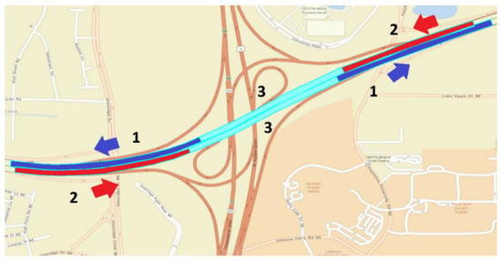
Figure 1.
Definition of three segment types at an interchange: (1) merging in blue, (2) diverging in red, and (3) within in cyan.
Table 1 also includes weather data that was obtained from Weather Underground [19]. The four major features of weather data collected are precipitation rate, precipitation accumulation, gust, and wind speed. The Weather Underground contains tabulated datasets of weather taken from localized weather stations at varying rates, these intervals range from five to fifteen minutes. Data from all weather stations surrounding I-285 were obtained over the same eight-month study period. The weather data was matched with crash both temporally and spatially. Specifically, weather stations were spatially paired with crashes through the implementation of a Voronoi diagram in Figure 2.
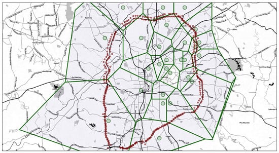
Figure 2.
Voronoi diagrams of weather stations.
As shown in Figure 2, the weather stations are depicted in larger green circle and the traffic cameras in smaller red circle. The Voronoi diagram was constructed around the weather stations to ensure that each crash was geographically assigned to the nearest weather station for obtaining concurrent weather information.
The driver-related factors or features are shown in Table 2, including the age of the driver at fault and one-hot-encoded categorical variables, such as reckless driving, driving under the influence and following too closely, as reported by the responding police officer for each accident. Finally, the distribution of multi-vehicle crash types is shown in Figure 3. As expected, rear-end collision is the dominating crash type on the interstate, followed by same-direction sideswipe and angle.
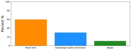
Figure 3.
The distribution of multi-vehicle crash types.
To gain an understanding of how the features correlate with one another, correlation matrices were generated with correlation coefficients shown in Figure 4 and Figure 5, respectively for RTWE features and driver-related features. The correlations among the features in each feature set are relatively low.
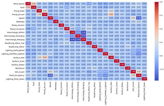
Figure 4.
Correlations of RTWE features.
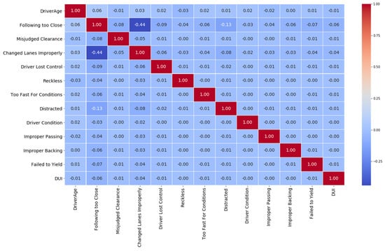
Figure 5.
Correlations of driver-related features.
4. Research Approach
Different from conventional statistical approaches, we studied the multi-vehicle crash types as a classification problem and explored two modern machine learning techniques, specifically Linear Discriminant Analysis (LDA) and eXtreme Gradient Boosting (XGBoost), which are the state-of-the-art classification algorithms under supervised learning. The main reason for picking LDA, a linear classifier, is for comparison with XGBoost. The classes or labels in this setting are three major multi-vehicle crash types on freeways, i.e., rear end, same-direction sideswipe, and angle. As described in Section 3, we have two feature sets. One includes road, traffic, weather, and environmental features (Table 1). The other includes driver-related features (Table 2). By applying the LDA, we sought to find hyperplanes or linear combinations of factors in lower-dimensional feature space to separate the three crash types. In comparison, XGBoost is a nonlinear tree-based ensemble method, which has proven to be an extremely effective algorithm and won many machine learning competitions. For example, Maksims Volkovs, Guangwei Yu, and Tomi Poutanen implemented gradient boosting models and won the first place of the 2017 ACM RecSys challenge [21]. Vlad Sandulescu and Mihai Chiru also implemented an XGBoost model that won the 2016 KDD Cup competition [22], which outperformed the statistical mixed model on the same set of features. Both LDA and XGBoost are introduced subsequently, followed by our data analysis results in the following section.
4.1. Linear Discriminant Analysis
LDA is a supervised machine learning technique that assumes Gaussian distribution and the same variance–covariance matrix (i.e., homoscedasticity) across classes. Modern LDA emerged from Fisher’s work published in 1936 [23]. The primary focus of LDA is to find k-1 projections or corresponding hyperplanes to separate k classes. In practice, LDA is commonly employed to reduce the dimensionality of large feature spaces.
4.2. Decision Tree Analysis
Decision trees are popular supervised methods in machine learning. Construction of decision trees involves guided decisions on answering sequential questions, such as which feature to split and at what value to split at each decision step to minimize regression error (regression trees) or classification error (classification trees). By making such decisions, tree-based models essentially partition the feature space in a nonlinear fashion into relatively homogenous regions for targeted outcomes. The major advantages of tree-based methods lie in their computational efficiency and flexibility in handling various types of features (e.g., numeric, ordinal, categorical, etc.). However, rudimentary decision trees suffer from high variance. In other words, small changes in data would result in different sequences of splits. In addressing this issue, bagging has been used that takes the average of predictions from many trees estimated with bootstrapped samples. This technique allows us to grow deep trees with high variance and low bias, and then averaging these trees to reduce variance. Bagging also provides a side benefit for free since each bagged tree makes use of about two-thirds of the data, leaving the remaining one-third of the data, referred to as out of the bag (OOB), for model validation. Although bagging has proved itself as a powerful technique for improving model accuracy, bootstrapping from the same training data set would likely result in similar or correlated trees. Random forests rise as an improvement over bagged trees by imposing a small tweak on selecting split features. For each split, instead of picking a predictor from the entire set of features, a random sample of features is considered as split candidates. This added randomness helps to decorrelate the trees and averaging of these decorrelated trees results in more reliable predictions. Random forests can be considered as a generalization of bagging. When the choice set of the split features is the same as the entire feature set, random forests reduce to bagging. Both bagging and random forests are ensemble methods since they take advantage of aggregating many tree models. With bootstrap sampling, these trees are constructed independently in parallel. Thus, bagging and random forests are considered as parallel ensemble methods. In contrast, boosting trees do not involve bootstrap sampling and are constructed sequentially, i.e., each tree is grown using information from previously grown trees. This sequential ensemble method permits the addition of new trees that correct the errors made by the trees previously constructed. In recent years, gradient boosting decision trees have emerged to dominance among machine learning competitions, as previously noted. By leveraging the distributed computing environments, XGBoost is an optimized distributed gradient boosting library designed to be highly efficient, flexible, and portable [3]. Specifically, XGBoost has a natural way to handle missing data and is well suited for analyzing crash-related features that are inherently heterogeneous. In this study, we used the open-source package, XGBoost, for model estimation. Different from conventional first-order tree-based methods, XGBoost is a second-order method with an objective function expressed in Equation (1), where the first term represents the second-order approximation of loss after removing the constant term, and the second and third terms are regularization terms to control the tree complexity.
where gamma (γ) represents the regularization on the number of nodes (T) and λ is the regularization on the sum square of leaf scores or weights. Both terms control the penalty imposed on tree complexity. is the weight or score for leaf j and represents the partitioning or node assignment function. Lastly, and are the first-order and second-order gradient statistics on the loss function, defined in Equations (2) and (3), where is the prediction for i-th instance at (t − 1) iteration and is the corresponding label.
The weight for each leaf is calculated using Equation (4). Where is the set of indices of data points assigned to the j-th leaf.
XGBoost recursively chooses a feature split that maximizes the gain (or reduction in loss). The detailed derivation of XGBoost can be found in [3]. For a better interpretation of XGBoost results, we implemented the Shapley Additive Explanation (SHAP) package [24]. Lundberg et al. [25] showed how SHAP values can be efficiently computed for tree-based ensemble models. Specifically, the SHAP value for each feature represents the feature’s contribution to the final model prediction, weighed against all other feature contributions, and can be computed from Equation (5).
where M is the number of features, x is the original feature space. denotes the set of observed features. is the expected value of the model prediction conditional on the set of features (S) being examined. is the expected value of model prediction in the absence of feature i. For the nonlinear models, such as XGBoost, the order in which features are introduced matters. is the Shapley Additive Explanation (SHAP) for feature i averaged across all possible feature orderings of the model.
The application of the SHAP values allows us to evaluate the influence of each feature value consistently and explicitly with the complex XGBoost model structure. The impact of each feature value over the multitude of decision trees was summed to ascertain the overall effect on ensembled model prediction. Therefore, the effect of each feature value could potentially be associated with an increased/decreased likelihood of a particular class prediction. Understanding such directional influence of each feature is pertinent to a better interpretation of tree-based ensemble models.
5. Data Analysis
A 60/40 data split was adopted for training and testing of both LDA and XGBoost models. Specifically, two models were developed in each model category for two feature sets: RTWE features and driver-related features.
5.1. LDA Results
The LDA models have a classification accuracy of 55.2% for RTWE features and 70.6% for driver-related features, evaluated on the test data sets. The LDA classification results are shown in Figure 6a and 6b for RTWE features and driver-related features, respectively. The mingling data points in Figure 6a indicate that the three crash types are not linearly separable in the RTWE feature space. Nonetheless, the top three features were identified as speed, vehicle count, and within-interchange locations, as shown in Table 5. However, in the driver-related feature space (Figure 6b), the clusters show some marginal levels of linear separability along the LD1 axis. Rear-end crashes mostly fall on the negative side of the LD1 axis while sideswipe and angle crashes fall on the positive side of the LD1 axis. The most influential features are following too close, changed lanes improperly and distracted driving, as seen by their high loading factors in Table 6.
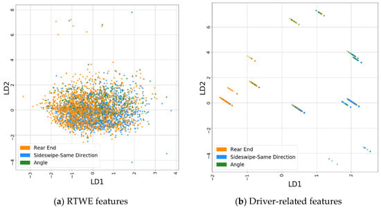
Figure 6.
Projection of crash data in the two Linear Discriminant Analysis (LDA) axes; (a) results for RTWE feature set, (b) results for driver-related feature set.

Table 5.
Loading factors for RTWE features.

Table 6.
Loading factors for driver-related features.
5.2. Gradient Boosting Modeling
In this study, two gradient boosting models were developed based on the two feature sets previously described. The models were developed using the XGBoost package [3]. XGBoost has several hyperparameters for tuning. The typical approach for hyperparameter tuning is the grid searching of the hyperparameter space based on cross-validation. However, this approach is computationally demanding when the hyperparameter space is large. For this study, we used Hyperopt [26], which adopted a meta-modeling approach to support automated hyperparameter optimization. The main hyperparameter values selected for our gradient boosting models are shown in Table 7.

Table 7.
Tuned eXtreme Gradient Boosting (XGBoost) hyperparameters.
5.2.1. Results on RTWE Features
As an ensemble method, the structure of a gradient boosting model can be challenging to visualize. XGBoost predictions are engendered from the culmination of a large number of sequential boosting trees, which are not straightforward to display. For visualization purposes, a single decision tree was constructed to demonstrate a representative tree structure and is shown in Figure 7.
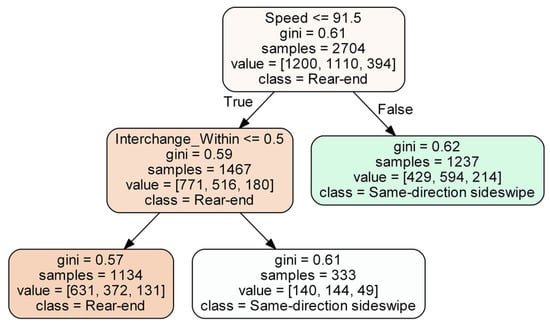
Figure 7.
Illustration of a single decision tree for RTWE features.
Figure 7 illustrates how a classification tree partitions the feature space. For the XGBoost model, which consists of a large number of sequential boosting trees, it would be extremely difficult, if not impossible, to plot them and interpret the results directly. Instead, SHAP values introduced previously was used to attribute feature contribution. The influential features are shown in Figure 8 in descending order of influence according to the mean SHAP values. As a result, our estimated XGboost model based on RTWE features achieved an accuracy of 68.4% on the test data set.
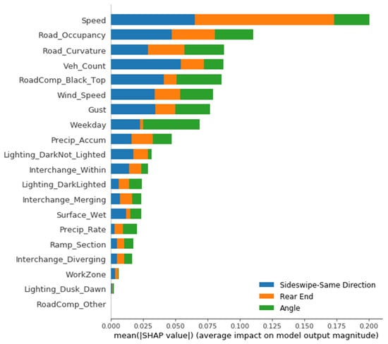
Figure 8.
Influence of RTWE features on crash types.
As shown in Figure 8, the top five features are speed, road occupancy, radius of curvature of the road, vehicle count, and black-top road composition. The plot also displays how relevant each feature is to each of the three crash types as indicated by colors. For instance, wet surface and black-top road compositions have a larger impact on angle and same direction sideswipe (SDS) crashes than on rear-end crashes. However, Figure 8 provides no information about if a feature is positively or negatively related to each crash type. To understand this directional relationship, SHAP values, representing the influence of features on the predictions of each class, are plotted in Figure 9 for all three crash types. The overall influence of a feature is indicated by their position on the vertical axis, which is in descending order from top to bottom. The horizontal axis shows the computed SHAP value (i.e., directional impact) of each feature for each class prediction. The color indicates the feature value from high (red) to low (blue). For example, the ‘Speed’ feature in Figure 9a is the most influential feature for the rear-end collision. The opposite direction between the color distribution and the SHAP axis (i.e., higher speeds (red) on the negative side of the axis and lower speeds (blue) on the positive side of the axis) indicates a negative correlation of speed with rear-end crashes. In other words, rear-end crashes more likely to involve vehicles with lower speeds. In contrast, speed remains the top influencer for SDS and angle crashes with a positive correlation, i.e., SDS and angle crashes likely involves vehicles with higher speeds.
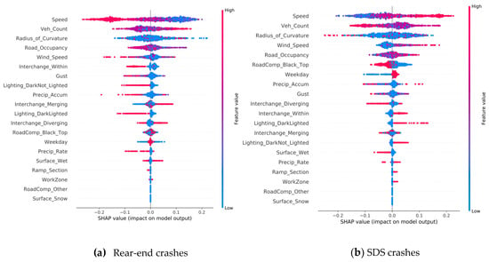
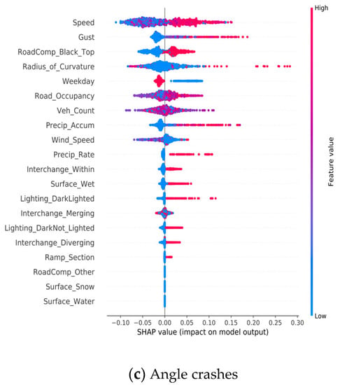
Figure 9.
Effects of RTWE features; (a) SHAP value plot for rear-end crashes, (b) SHAP value plot for SDS crashes, (c) SHAP value plot for angle crashes (note: red indicates high feature value and blue indicates low feature value).
Road features have a unique impact on crash types. The within-interchange locations (Interchange_Within) appear to have a higher chance for SDS and angle crashes, while merging locations (Interchange_Merging) are correlated with rear-end collisions. Ramp sections have a higher chance for both angle and SDS crashes. The composition of the road (i.e., surface type) also appears to impact the crash types. The black-top roads (asphalt pavement) have a positive association with angle crashes and a negative association with SDS crashes. This infers that SDS more likely occur on white-top (concrete) roads. Weather factors play an important role in crash types. Higher precipitation/wet surface and gust appear to be attributable factors to angle crashes. The lighting condition also affects crash types differently. Rear-end crashes happened more often in the daylight, while SDS and angle crashes occur more frequently at night with both dark-not-lighted and dark-lighted conditions. The angle and SDS crashes often occur on weekends. In addition, workzone is correlated with SDS crashes and the curvature of the road is correlated with angle crashes.
5.2.2. Results on Driver-Related Features
Similar to the single-tree model for the RTWE feature set, we also constructed a single tree model for the driver-related feature set for illustration purposes, as shown in Figure 10.
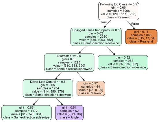
Figure 10.
Illustration of a single decision tree for driver-related features.
For the driver-related features, our estimated XGBoost model resulted in increased accuracy of 80.2% on the test data set. This is not surprising as driver-related features have more direct impacts on the modes of collision than the RTWE features. The influential features are shown in descending order in Figure 11.
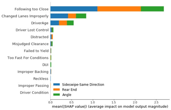
Figure 11.
Influence of driver-related features on crash types.
The top three features (i.e., following too close, changed lanes improperly, and driver age) dominate the utility of this model. There is an intuitive and logical connection between following too closely and improperly changing lanes with both rear-end and SDS crashes, as indicated by the longer bars in blue and orange in Figure 11. In addition, SHAP values were computed for each collision type and are plotted in Figure 12.
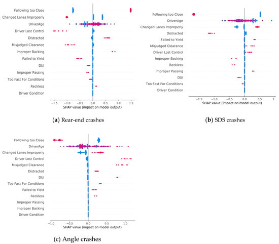
Figure 12.
Effects of driver-related features; (a) SHAP value plot for rear-end crashes, (b) SHAP value plot for SDS crashes, (c) SHAP value plot for angle crashes (note: red indicates high feature value and blue indicates low feature value).
As shown in Figure 12, older drivers appear to be more likely involved in rear-end crashes than SDS crashes as it would be easier to judge on potential encroachment of adjacent vehicles than time headway of the preceding vehicle on freeways. Angular crashes are relatively rare on freeways and typically related to driving under the influence (DUI) and speeding. Misjudged clearance, losing control, and improperly changing lanes contributed to both angle and SDS crashes. Additionally, following too close and distracted driving are two major factors for rear-end crashes, which seems to be intuitive in light of rising cellular usage on road.
6. Discussion
Crash data has traditionally been analyzed using classic statistical models, such as nested logit, mixed logit, and discrete mixture models. The statistical models often impose strong assumptions on error distribution and correlation and are suitable for data sets with limited features. In this study, we demonstrated the utility of modern machine learning techniques with a fused data set that contains a relatively large number of features. Two sets of features, i.e., RTWE features and driver-related features, were investigated to gain a deeper understanding of how these features potentially related to a particular type of crash, which is a classification problem in a machine learning context. Specifically, two modern machine learning techniques (i.e., LDA and XGboost) were explored to mine a comprehensive data set fused from four distinct data sources. As a result, LDA has limited capacity in classifying the crash types due to its restrictive assumptions. XGBoost models, on the other hand, are nonlinear and able to classify the crash types in a reasonably accurate manner. The XGBoost models were able to achieve the test accuracy levels of 68.4% and 80.2% with the RTWE features and driver-related features, respectively. A potential drawback of XGBoost models is their lack of interpretability. This issue was mitigated by implementing Shapley Additive Explanation (SHAP) value [23]. Additionally, compared to the classic statistical methods, the tree-based ensemble methods require additional efforts on hyperparameter fine-tuning.
Based on the XGBoost model developed using the RTWE features, it was found that within-interchange locations have a lower chance of rear-end crashes, but a higher propensity for SDS and angle crashes. Merging locations correlate positively with rear-end crashes. Ramp section was positively correlated with both angle and SDS crashes. Angle crashes displayed a higher reactivity to adverse weather conditions, such as precipitation and wet surface. Higher wind speed appears to increase the chance of SDS crashes. Additionally, angle crashes occurred more frequently on weekends, likely due to more aggressive driving. SDS and angle crashes happened more often in dark and low light conditions, likely due to low visibility. Workzone is mainly associated with SDS crashes. Compared to RTWE features, a better classification result was obtained using driver-related features, which is expected because driver-related features, especially driver faults, have a direct impact on crash types. As a result, rear-end crashes were commonly caused by following too close and distracted driving, while angle and SDS crashes were typically related to improperly changing lanes, losing control, misjudged clearance, and failing to yield. In particular, driving under the influence (DUI) is a salient feature for angle crashes, which often occurred on weekend. Additionally, older drivers are more likely to be involved in rear-end crashes, while younger drivers had a relatively higher representation in angle and SDS crashes.
Besides the inspiring results from this study, we would like to point out some limitations that could be addressed by future studies. Given the data-driven nature of machine learning methods, the quality of data is essential to and governs the quality of the resulting models. Although four different sources of data have been fused and used for this study. The data set is still quite limited and localized. The expansion of the geographical coverage of the data set would be desirable. In addition, the data set can be further augmented by including other newly available data sources, such as real-time road conditions and vehicle operating data. Given the various sensors being deployed along with the transportation infrastructure (e.g., intelligent transportation systems and road weather information systems) and within vehicles (e.g., connected and automated vehicles), collecting and fusing these high-resolution real-time data sources become practically possible. These additional data sources can certainly be utilized to construct even more powerful machine learning models to better understand crash patterns and mechanisms. For this study, we focused on understanding the various features underlying different crash patterns or types. As such, only crash-related data were mined. The results of this study cannot be used to directly infer the likelihood of crashes and corresponding attributing factors. Future studies that consider sampling non-crash conditions are necessary to construct predictive models for crash occurrence and frequency. Again, leveraging the modern machine learning methods and increasingly available high-resolution data sources for predicting crashes is a promising area and expected to produce much more accurate and reliable results than the existing models based on conventional regression methods (e.g., zero-inflated Poisson models, negative binomial models, etc.). Additionally, to estimate the probability of crash occurrence as well as crash types, a more generic hierarchical model structure could be adopted to estimate crash probability at a higher level and then model crash types and/or severities at a lower level.
7. Conclusions
Traditionally, crash data has been studied with classic statistical methods as opposed to machine learning techniques. Crash data is often analyzed to engender inferences about the underlying mechanism or relationship. This inference can be used to create countermeasures to mitigate or reduce the risk of collisions. Historically, it has been thought that machine learning techniques should be implemented when the prediction is more important than interpretation. However, new methods, such as the Shapley Additive Explanation [24], have demonstrated that complex machine learning models, such as gradient boosting decision trees, can be properly interpreted, making it a more versatile technique within various modeling communities. Additionally, machine learning methods are more adept at managing diverse and elaborate data sets. Crash data contains a vast quantity of various features, which are well suited for and potentially better analyzed by modern machine learning techniques as compared to traditional statistical methods.
In this study, we explored and contrasted two modern machine learning techniques (i.e., LDA and XGBoost) by mining a uniquely comprehensive data set fused from four distinct data sources. The objective of the study is two-fold: (1) demonstrate the utility and versatility of the modern machine learning methods, and (2) better understand the effects and intricate relationships of both RTWE features and driver-related features underlying three common freeway collision types: (1) rear-end collision, (2) same-direction sideswipe collision, and (3) angle collision. As a result, many feature effects agree well with those found from previous studies. The high model accuracies with the test data sets are particularly interesting and inspiring, and underscore the superiority and high potential of the XGBoost method in the context of crash analysis and modeling.
Author Contributions
The authors confirm contribution to the paper as follows: Study conception and design, J.J.Y.; data collection, analysis, and interpretation of results, C.M. and J.J.Y.; draft manuscript preparation, C.M. and J.J.Y.; draft manuscript review and editing: J.J.Y. and C.M. All authors reviewed the results and approved the final version of the manuscript.
Funding
This research received no external funding.
Acknowledgments
The authors would like to thank the Georgia Department of Transportation (GDOT) for providing crash data and access to the GDOT Navigator system’s real-time traffic data.
Conflicts of Interest
The authors declare no conflict of interest.
References
- The World Health Organization. Global Health Observatory (GHO) Road Safety Data. 2016. Available online: https://www.who.int/gho/road_safety/en/ (accessed on 1 March 2020).
- Karlaftis, M.G.; Vlahogianni, E.I. Statistical methods versus neural networks in transportation research: Differences, similarities and some insights. Transp. Res. Part C 2011, 19, 387–399. [Google Scholar] [CrossRef]
- Chen, T.; Guestrin, C. XGBoost: A Scalable Tree Boosting System. In Proceedings of the 22nd SIGKDD Conference on Knowledge Discovery and Data Mining, San Francisco, CA, USA, 13–17 August 2016. [Google Scholar]
- Razi-Ardakani, H.; Mahmoudzadeh, A.; Kermanshah, M. A Nested Logit analysis of the influence of distraction on types of vehicle crashes. Eur. Transp. Res. Rev. 2018, 10, 44. [Google Scholar] [CrossRef]
- Neyens, D.M.; Boyle, L.N. The effect of distractions on the crash types of teenage drivers. Accid. Anal. Prev. 2007, 39, 206–212. [Google Scholar] [CrossRef]
- El Faouzi, N.-E.; Billot, R.; Nurmi, P.; Nowotny, B. Effects of Adverse Weather on Traffic and Safety: State-of-the-art and a European Initiative. In Proceedings of the SIRWEC International Road Weather Conference, Quebec, QC, Canada, 5–7 February 2010. [Google Scholar]
- Daniel, J.R.; Chien, S.I. Impact of Adverse Weather on Freeway Speeds and Flows. In Proceedings of the 88nd Annual Meeting of the Transportation Research Board, Washington DC, USA, 11–15 January 2009; Transportation Research Board of the National Academies: Washington, DC, USA, 2009. [Google Scholar]
- Khattak, A.; Kantor, P.; Council, F. Role of adverse weather in key crash types on limited-access: Roadways implications for advanced weather systems. Transp. Res. Rec. J. Transp. Res. Board 1998, 1621, 10–19. [Google Scholar] [CrossRef]
- Kim, D.-G.; Lee, Y.; Washington, S.; Choi, K. Modeling crash outcome probabilities at rural intersections: Application of hierarchical binomial logistic models. Accid. Anal. Prev. 2007, 39, 125–134. [Google Scholar] [CrossRef] [PubMed]
- McFadden, D.; Train, K. Mixed mnl models of discrete response. J. Appl. Econom. 2000, 15, 447–470. [Google Scholar] [CrossRef]
- Chu, A.A.-I. A Comprehensive Mixed Logit Analysis of Crash Type Conditional on a Crash Event. Ph.D. Thesis, The University of Texas at Austin, Austin, TX, USA, 2015. [Google Scholar]
- Pai, C.W.; Hwang, K.P.; Saleh, W. A mixed logit analysis of motorists’ right-of-way violation in motorcycle accidents at priority T-junctions. Accid. Anal. Prev. 2009, 41, 565–573. [Google Scholar] [CrossRef] [PubMed]
- Dong, B.; Ma, X.; Chen, F.; Chen, S. Investigating the Differences of Single-Vehicle and Multivehicle Accident Probability Using Mixed Logit Model. J. Adv. Transp. 2018, 2018, 2702360. [Google Scholar] [CrossRef] [PubMed]
- McCartt, A.T.; Northrup, V.S.; Retting, R.A. Types and characteristics of ramp-related motor vehicle crashes on urban interstate roadways in Northern Virginia. J. Saf. Res. 2004, 35, 107–114. [Google Scholar] [CrossRef] [PubMed]
- Hong, J.; Tamakloe, R.; Park, D. A Comprehensive Analysis of Multi-Vehicle Crashes on Expressways: A Double Hurdle Approach. Sustainability 2019, 11, 2782. [Google Scholar] [CrossRef]
- Abdel-Aty, M.A.; Abdelwahab, H.T. Predicting injury severity levels in traffic crashes: A modeling comparison. J. Transp. Eng. 2004, 130, 204–210. [Google Scholar] [CrossRef]
- Ramani, R.G.; Shanthi, S. Classification of Vehicle Collision Patterns in Road Accidents using Data Mining Algorithms. Int. J. Comput. Appl. 2011, 35, 30–37. [Google Scholar]
- López, G.; de Oña, J.; Joaquínc, A. Using Decision Trees to extract Decision Rules from Police Reports on Road Accidents. Soc. Behav. Sci. 2012, 53, 106–114. [Google Scholar]
- The Weather Underground Atlanta, GA Weather Conditions. 2020. Available online: https://www.wunderground.com (accessed on 1 March 2020).
- National Highway Safety Administration. Critical Reasons for Crashes Investigated in the National Motor Vehicle Crash Causation Survey; National Center for Statistics and Analysis: Washington, DC, USA, 2015. [Google Scholar]
- Volkovs, M.; Yu, G.W.; Poutanen, T. Content-based Neighbor Models for Cold Start in Recommender Systems. In Proceedings of the Recommender Systems Challenge 2017, Como, Italy, 27 August 2017; p. 6. [Google Scholar] [CrossRef]
- Sandulescu, V.; Chiru, M. Predicting the future relevance of research institutions—The winning solution of the KDD Cup 2016. arXiv 2016, arXiv:1609.02728v1. [Google Scholar]
- Fisher, R.A. The Use of Multiple Measurements in Taxonomic Problems. Ann. Eugen. 1936, 7, 179–188. [Google Scholar] [CrossRef]
- Lee, S.-I.; Lundberg, S. An unexpected unity among methods for interpreting model predictions. arXiv 2016, arXiv:1611.07478. [Google Scholar]
- Lundberg, S.M.; Erion, G.G.; Lee, S.-I. Consistent Individualized Feature Attribution for Tree Ensembles. arXiv 2019, arXiv:1802.03888v3. [Google Scholar]
- Bergstra, J.; Yamins, D.; Cox, D.D. Making a Science of Model Search: Hyperparameter Optimization in Hundreds of Dimensions for Vision Architectures. In Proceedings of the 30th International Conference on Machine Learning (ICML 2013), Atlanta, GA, USA, 16–21 June 2013. [Google Scholar]
© 2020 by the authors. Licensee MDPI, Basel, Switzerland. This article is an open access article distributed under the terms and conditions of the Creative Commons Attribution (CC BY) license (http://creativecommons.org/licenses/by/4.0/).