Machine Learning Traffic Flow Prediction Models for Smart and Sustainable Traffic Management

Abstract

Sustainable traffic management relies on accurate traffic flow prediction to reduce congestion, fuel consumption, and emissions and minimise the external environmental impacts of traffic operations. This study contributes to this objective by developing and evaluating advanced machine learning models that leverage multisource data to predict traffic patterns more effectively, allowing for the deployment of proactive measures to prevent or reduce traffic congestion and idling times, leading to enhanced eco-friendly mobility. Specifically, this paper evaluates the impact of multisource sensor inputs and spatial detector interactions on machine learning-based traffic flow prediction. Using a dataset of 839,377 observations from 14 detector stations along Melbourne’s Eastern Freeway, Bidirectional Long Short-Term Memory (BiLSTM) models were developed to assess predictive accuracy under different input configurations. The results demonstrated that incorporating speed and occupancy inputs alongside traffic flow improves prediction accuracy by up to 16% across all detector stations. This study also investigated the role of spatial flow input interactions from upstream and downstream detectors in enhancing prediction performance. The findings confirm that including neighbouring detectors improves prediction accuracy, increasing performance from 96% to 98% for eastbound and westbound directions. These findings highlight the benefits of optimised sensor deployment, data integration, and advanced machine-learning techniques for smart and eco-friendly traffic systems. Additionally, this study provides a foundation for data-driven, adaptive traffic management strategies that contribute to sustainable road network planning, reducing vehicle idling, fuel consumption, and emissions while enhancing urban mobility and supporting sustainability goals. Furthermore, the proposed framework aligns with key United Nations Sustainable Development Goals (SDGs), particularly those promoting sustainable cities, resilient infrastructure, and climate-responsive planning.

1. Introduction

Sustainable traffic management relies on accurate short-term traffic flow prediction to optimise road network performance, reduce congestion, and minimise environmental impact. Effective forecasting enables proactive traffic control, improving mobility while lowering fuel consumption and emissions. However, due to the non-linear dynamics of traffic flow, accurately predicting flow patterns within short horizons, up to 1 h into the future, remains challenging. These complexities impact the prediction accuracy for short-term forecasting, with significant implications for intelligent transportation system (ITS) applications [1,2]. Although considerable research has been undertaken to improve prediction accuracy for ITS, challenges continue in achieving reliable accuracies across varying traffic conditions.

While traditional models like ARIMA and Kalman Filter have been widely used, they often struggle with capturing non-linear dependencies and adapting to diverse traffic conditions. Traditional models like ARIMA, Kalman Filter, and simple neural networks have limitations when predicting traffic data, especially when dealing with multiple input variables such as speed, flow, and occupancy. ARIMA and Kalman Filter rely on linear assumptions and are typically suited for single-variable or simple multivariable time series, making them unable to capture the complex, non-linear relationships and sudden fluctuations characteristic of traffic systems. While the Kalman Filter works well for real-time noise reduction, it struggles with long-term forecasting and modelling non-linear dynamics. Moreover, simple feedforward neural networks can model non-linear relationships but lack the ability to capture temporal dependencies naturally, treating inputs independently without considering the sequential nature of traffic flow. In contrast, BiLSTM networks are specifically designed to handle time-series data with long-term dependencies, capturing both past and future temporal patterns due to their bidirectional architecture. They perform better at modelling complex, non-linear interactions between multiple variables, making them significantly more effective for predicting traffic conditions in dynamic, real-world scenarios [3]. In the authors’ previous study [4], they compared the performance, fault tolerance, and transferability of several machine learning models, including Recurrent Neural Networks (RNNs), Elman networks, unidirectional Long Short-Term Memory (LSTM), Deep Learning Backpropagation (DLBP), and Bidirectional LSTM (BiLSTM), using traffic flow and speed data from Melbourne’s Eastern Freeway. That evaluation concluded that BiLSTM models consistently outperformed the others, particularly under data corruption or noise scenarios. Therefore, this study builds on that foundation by focusing exclusively on the BiLSTM model and seeking to enhance its predictive performance by optimising input configurations.

This study specifically examines the impact of different input configurations on the accuracy of short-term traffic flow predictions, focusing on the BiLSTM model’s performance. A large dataset was utilised, comprising data from multiple detector stations along Melbourne’s Eastern Freeway in Melbourne, Australia. This dataset, collected over a 31-day period (1 min intervals), includes 839,377 observations tested from 14 cleaned detectors for short-term traffic flow prediction for both travel directions. These observations were collected for 31 days, and they represent diverse and complex traffic characteristics, such as peak, non-peak, weekday, weekend, incident, and non-incident information, to capture a broad spectrum of traffic conditions.

This study has two primary objectives. First, it evaluates the effect of different combinations of input variables, such as flow, speed, and occupancy, on the predictive accuracies for 14 detectors for eastbound and westbound travel directions. Second, it explores the influence of spatial interactions by incorporating data from upstream and downstream detectors, assessing whether data from neighbouring detectors can enhance prediction accuracies. This analysis ultimately seeks to identify optimal input configurations for short-term traffic flow prediction, aiming to enhance model adaptability to the diverse and complex traffic patterns encountered in real-world applications.

By optimising traffic flow predictions with data-driven, adaptive models, this research contributes to developing sustainable road networks that are more efficient and environmentally conscious. This study offers insights for designing intelligent, sustainable transportation systems through machine learning and advanced sensor integration.

2. Related Literature

Accurate traffic prediction plays an important role in the effectiveness of ITS, particularly in urban environments where congestion presents a significant challenge. Congestion can be classified into two types: recurrent, such as routine peak-hour traffic, and non-recurrent, which includes incidents like accidents, adverse weather conditions, or roadworks (e.g., incidents such as crashes, severe weather conditions, or road maintenance) [5,6,7,8]. Non-recurrent events are especially problematic due to their unpredictable and complex nature [9,10]. Traditional approaches such as the California Algorithm [11] and statistical models like Autoregressive Integrated Moving Average (ARIMA) and Kalman Filters were commonly employed but proved insufficient in capturing the non-linear and dynamic characteristics of traffic flow, particularly on arterial roads [12,13]. This section reviews significant studies focusing on methodologies for traffic flow prediction.

2.1. Parametric Approaches

Parametric methods, such as ARIMA and Kalman Filters, depend on predefined mathematical structures that assume fixed relationships among traffic variables [14,15,16]. These approaches are effective for short-term traffic predictions under stable conditions but struggle to account for non-linear traffic dynamics [17,18,19]. For instance, ARIMA models are commonly used to forecast traffic speeds and volumes by analysing patterns in historical time-series data [20]. However, their performance declines in unpredictable scenarios, such as those caused by weather changes or incidents [12,21].

Despite these shortcomings, parametric models remain widely utilised in traffic prediction. Kalman Filters, in particular, are valuable for real-time traffic monitoring due to their ability to update predictions dynamically using incoming sensor data [22,23]. However, similar to ARIMA, their effectiveness diminishes in highly dynamic settings, such as arterial roads prone to frequent disruptions [24].

In order to address these challenges, newer approaches like the AdaBoost algorithm have been developed for real-time vehicle detection, enhancing the accuracy of incident detection and response [25]. Integrating such algorithms with nonparametric traffic prediction models provides a more robust solution, especially for urban arterial roads where weather and incidents significantly disrupt traffic flow.

2.2. Nonparametric Approaches

Unlike parametric models, nonparametric methods do not rely on a fixed model structure, allowing them to adapt more effectively to the non-linear characteristics of traffic patterns [26,27,28,29]. Techniques such as Neural Networks (NNs) and Support Vector Regression (SVR) have shown remarkable success in processing complex, multisource traffic data, particularly on arterial roads where traditional methods often fall short [30,31,32].

For example, NNs have demonstrated their ability to accurately predict traffic speed and volume by leveraging large datasets and adapting to fluctuating traffic conditions [33,34,35,36,37]. These models are particularly suited for real-time ITS applications, where rapid changes in traffic conditions demand flexibility.

Long Short-Term Memory (LSTM) networks, a specialised form of Recurrent Neural Networks (RNNs) [38,39,40,41], have become a leading tool in traffic forecasting. Their ability to model temporal dependencies in data makes them highly effective for capturing traffic patterns over time [42]. For example, LSTM models have also been used to monitor and evaluate sequential patterns in vehicular live load data collected through Weigh-In-Motion (WIM) systems, offering a consistent method for detecting anomalies and system drift over time [43]. LSTMs are especially advantageous on arterial roads, where external factors like weather and incidents can cause significant variability. LSTMs deliver more accurate and reliable predictions by integrating real-time sensor data than traditional parametric approaches [44].

2.3. LSTM Models for Traffic Prediction

Predicting short-term traffic conditions, typically up to 60 min ahead, is critical for the success of ITS, such as adaptive traffic management and travel advisory systems. LSTM networks have gained significant attention for traffic prediction because they can utilise real-world data from sources like inductive loop detectors, CCTV, and probe vehicles [45]. Designed to capture long-term dependencies in sequential data, LSTMs excel in forecasting traffic parameters such as speeds, flows, and travel times [42,46].

For instance, Ref. [45] demonstrated that LSTM models achieve greater speed prediction accuracy than traditional methods. Similarly, Ref. [44] highlighted the effectiveness of LSTMs for predicting irregular travel times, showing minimal errors in one-step-ahead forecasts. LSTMs have also been successfully applied to traffic flow predictions, delivering high accuracy across various time horizons. Research by [47,48] showed that LSTMs outperform other models in predicting speed and flow on different road types, including arterial roads, which experience more significant traffic variability.

Moreover, LSTM models have been employed in studies on car-following behaviour, providing insights into vehicle acceleration and deceleration across diverse road networks. These models are particularly beneficial in urban environments, where traffic patterns are influenced by external factors such as weather and incidents [45,49,50,51].

2.4. BiLSTM Models

Although LSTM models have demonstrated strong performance in traffic prediction, BiLSTMs offer an enhanced capability by learning temporal dependencies in both forward and backward directions. This bidirectional processing allows BiLSTM models to excel in predicting traffic speeds and flows, particularly under complex and variable traffic conditions. By accounting for bidirectional dependencies, BiLSTMs provide improved handling of the stochastic nature of traffic flow, resulting in more accurate predictions than their unidirectional counterparts [44].

For example, Ref. [47] proposed an end-to-end deep learning framework with BiLSTM layers for traffic flow forecasting. Their model effectively addressed overfitting challenges and accurately predicted various traffic scenarios. Similarly, a comparative study found that stacked BiLSTM architectures outperformed both Uni-LSTM and standalone BiLSTM models in forecasting network-wide traffic speeds [52].

In summary, while parametric models provide foundational methods for traffic prediction, their limitations in handling dynamic, non-linear data make them less suited to the complexities of urban roads. The flexibility and adaptability of LSTM and BiLSTM models, especially when paired with multisource data, allow them to handle real-time traffic variations more effectively. Therefore, this research focuses on utilising LSTM and BiLSTM models for traffic prediction by integrating data from multiple sources, including neighbouring detectors, to enhance the accuracy and resilience of traffic forecasting in urban settings.

3. Data Description

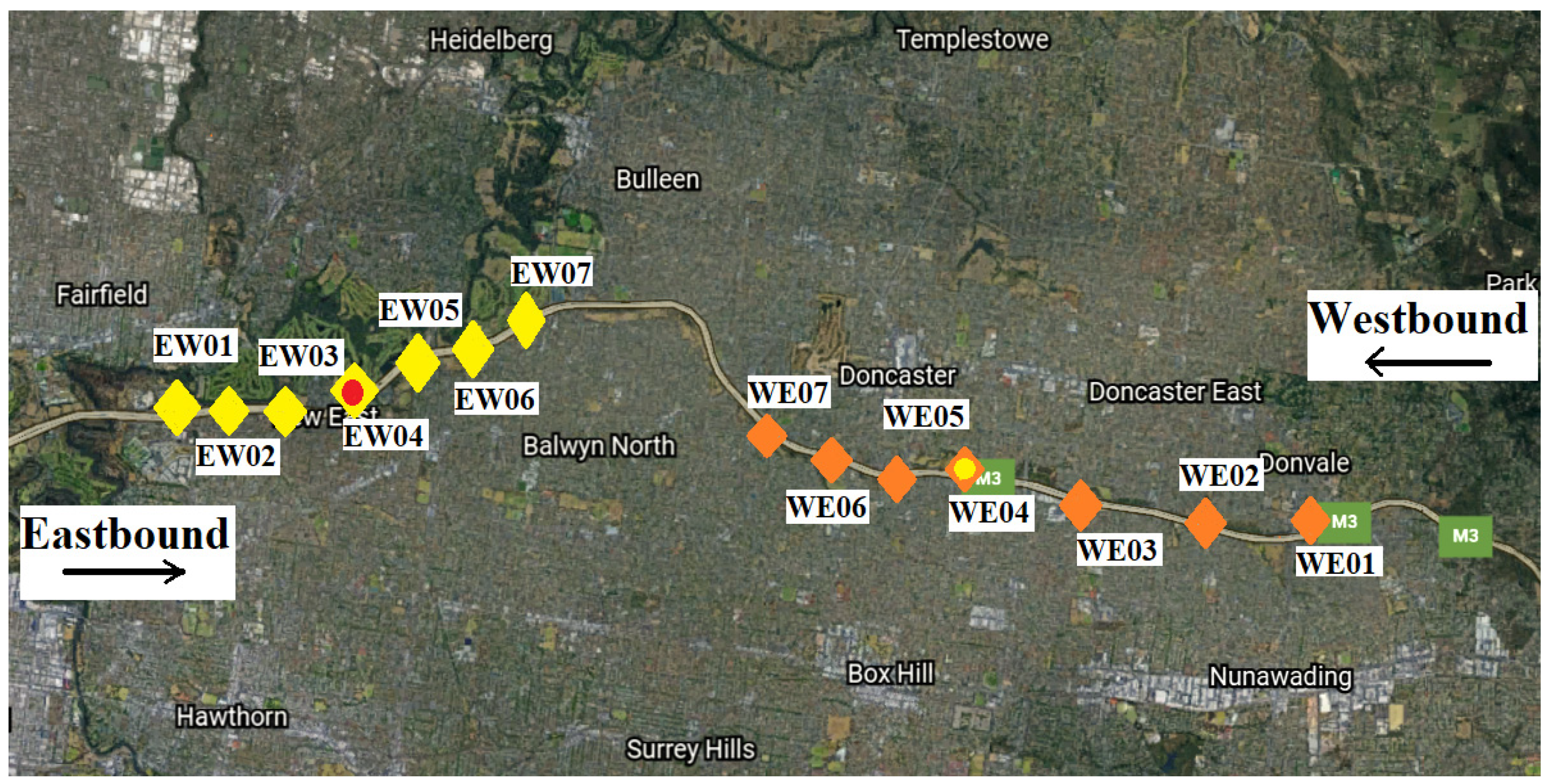
This study utilised real-world traffic data collected from inductive loop detectors installed along the Eastern Freeway in Melbourne, Australia. This 18-kilometre freeway extends between East Link at Nunawading (eastbound) and Alexandra Parade (westbound). The dataset comprised speed measurements recorded over 31 days, from 1 July to 31 July 2016, for eastbound (EB) and westbound (WB) directions. Data was aggregated at 1 min intervals across all lanes at each site for the entire 24 h period daily.

The information was sourced from multiple detectors distributed along the freeway’s mainline carriageway, with spacing between detectors ranging from 450 to 1070 m. Each detector provided approximately 42,000 data points for key traffic metrics: speed (km/h), flow (vehicle count), and occupancy (percentage of time vehicles occupy the detector). The data was split into two subsets for the analysis: 60% (25,200 observations) for model training and 40% (16,800 observations) for testing and validation.

Seven detector locations were selected in each direction, resulting in 14 locations covering the freeway’s length. Figure 1 illustrates the positioning of these detectors along the carriageway.

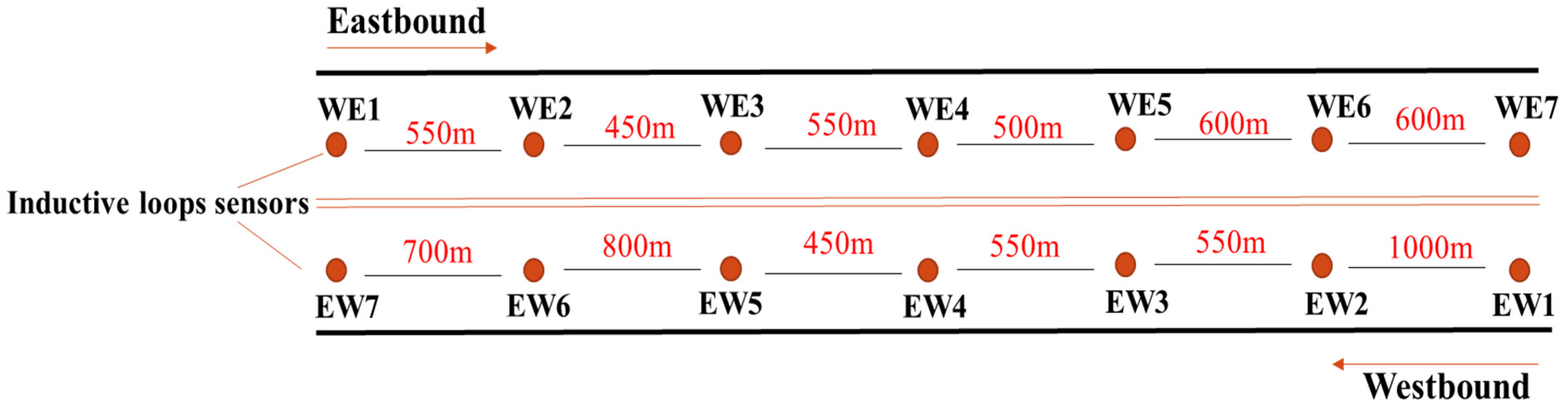
For model development, data was obtained from seven detection stations in the westbound direction (designated as EW1, EW2, EW3, EW4, EW5, EW6, and EW7). These stations were spaced sequentially at intervals of 550, 450, 550, 500, 600, and 600 m. Similarly, data was collected from seven detection stations in the eastbound direction (designated as WE1, WE2, WE3, WE4, WE5, WE6, and WE7). The spacing between the eastbound stations was approximately 1000, 550, 550, 450, 800, and 700 m. The layout of these detection stations is depicted in Figure 2.

Table 1. Data used for model development.

Location	Total Data Set
Eastern Freeway, Westbound	335,265 observations
Eastern Freeway, Eastbound	504,112 observations
Total	839,377 observations

summarises the total dataset used in both directions for the model development.

4. Methodology

The BiLSTM model was assessed using the earlier datasets. This model has demonstrated exceptional accuracy in forecasting traffic conditions in previous studies [47,48]. The BiLSTM architecture consists of four layers: a sequence input layer (with one feature), BiLSTM layers (300 hidden units), a fully connected layer (producing one response), and a regression layer.

Hyperparameters were selected through a preliminary grid search process to optimise the model. Several combinations of learning rate, number of hidden units, batch size, and training epochs were evaluated based on validation performance using mean absolute error (MAE) and root mean square error (RMSE) across a subset of detectors. The final configuration was chosen as it consistently achieved the lowest validation error and best generalisation performance. The selected hyperparameters are gradient decay factor (0.9), initial learning rate (0.005), minimum batch size (128), maximum epochs (300), training optimiser (Adaptive Moment Estimation Optimiser), learning rate schedule (Piecewise), learning rate drop period (125 epochs), and a learning rate drop factor (0.2).

The experiments utilised Matlab R2019b with the Deep Learning Toolbox functions, including trainNetwork, trainingOptions, and predictAndUpdateState [54].

5. LSTM and BiLSTM

LSTM is an advanced type of RNN designed to address the limitations of traditional RNNs [55,56,57,58]. RNNs often face challenges with vanishing or exploding gradients during training due to using backpropagation algorithms, which affect weight adjustments and make it challenging to model long-term dependencies effectively. In order to overcome this issue, LSTM was introduced.

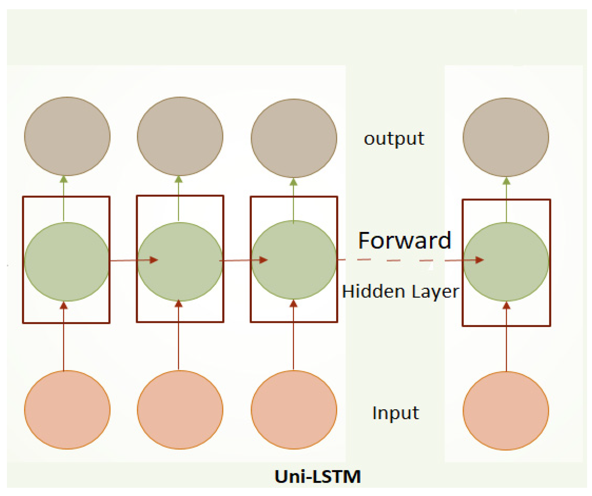
LSTM employs multiple gates—namely the input gate, output gate, and forget gate—which regulate the flow of information, ensuring that only relevant data is retained in the hidden layers and carried forward for predictions (see Figure 3). This architecture enables LSTM to capture long-term dependencies and outperform traditional RNN models in generating accurate predictions.

In these models, the predicted values are computed using the following equations [59]:

$$\mathrm{Input} \mathrm{gate} \left({\mathrm{I}}_{\mathrm{t}}\right)={\mathsf{\sigma }}_{\mathrm{g}}\left({\mathrm{W}}_{\mathrm{i}}{\mathrm{X}}_{\mathrm{t}}+{\mathrm{R}}_{\mathrm{i}}{\mathrm{h}}_{\mathrm{t}-1}+{\mathrm{b}}_{\mathrm{i}}\right)$$

(1)

$$\mathrm{Forget} \mathrm{gate} \left({\mathrm{f}}_{\mathrm{t}}\right)={\mathsf{\sigma }}_{\mathrm{g}}\left({\mathrm{W}}_{\mathrm{f}}{\mathrm{X}}_{\mathrm{t}}+{\mathrm{R}}_{\mathrm{f}}{\mathrm{h}}_{\mathrm{t}-1}+{\mathrm{b}}_{\mathrm{f}}\right)$$

(2)

$$\mathrm{Cell} \mathrm{state} \left({\mathrm{C}}_{\mathrm{t}}\right)={\mathsf{\sigma }}_{\mathrm{c}}({\mathrm{W}}_{\mathrm{c}}{\mathrm{X}}_{\mathrm{t}}+{\mathrm{R}}_{\mathrm{c}}{\mathrm{h}}_{\mathrm{t}-1}+{\mathrm{b}}_{\mathrm{c}})$$

(3)

$$\mathrm{Output} \mathrm{gate} \left({\mathrm{o}}_{\mathrm{t}}\right)={\mathsf{\sigma }}_{\mathrm{g}}\left({\mathrm{W}}_{\mathrm{o}}{\mathrm{X}}_{\mathrm{t}}+{\mathrm{R}}_{\mathrm{o}}{\mathrm{h}}_{\mathrm{t}-1}+{\mathrm{b}}_{\mathrm{o}}\right)$$

(4)

where

• σ_g represents the gate activation function.
• ${\mathrm{W}}_{\mathrm{i}},{\mathrm{W}}_{\mathrm{f}},{\mathrm{W}}_{\mathrm{c}},\mathrm{a}\mathrm{n}\mathrm{d} {\mathrm{W}}_{\mathrm{o}}$ are input weight matrices.
• $R_i,R_f,R_c,\mathrm{a}\mathrm{n}\mathrm{d} R_o$ are recurrent weight matrices
• $X_t$ is the input at time t.
• $h_{t-1}$ s the output from the previous time step (t − 1).
• $b_i,b_f,b_c,\mathrm{a}\mathrm{n}\mathrm{d} b_o$ are bias vectors.

The input gate determines which new information should be added to the cell state, while the forget gate controls the removal of previous memory from the cell state. The LSTM’s cell state and output at time t are calculated as follows:

Cell state:

Ct = ft⊙ct − 1 + it⊙gt

(5)

Hidden state:

Ht = ot⊙σc(ct)

(6)

where ⊙ denotes the Hadamard product, which is the element-wise multiplication of vectors.

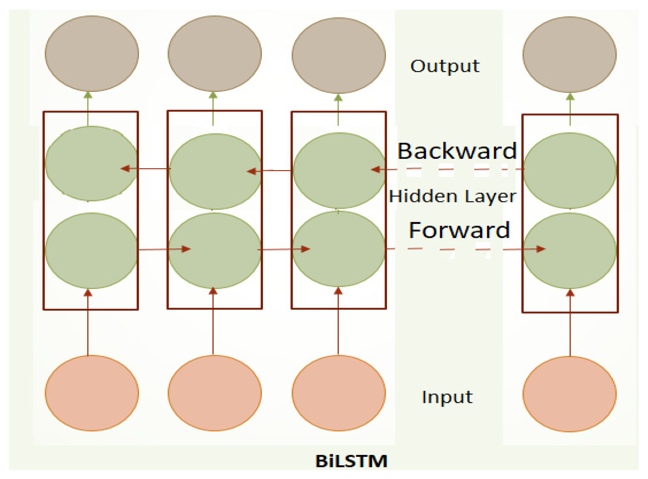
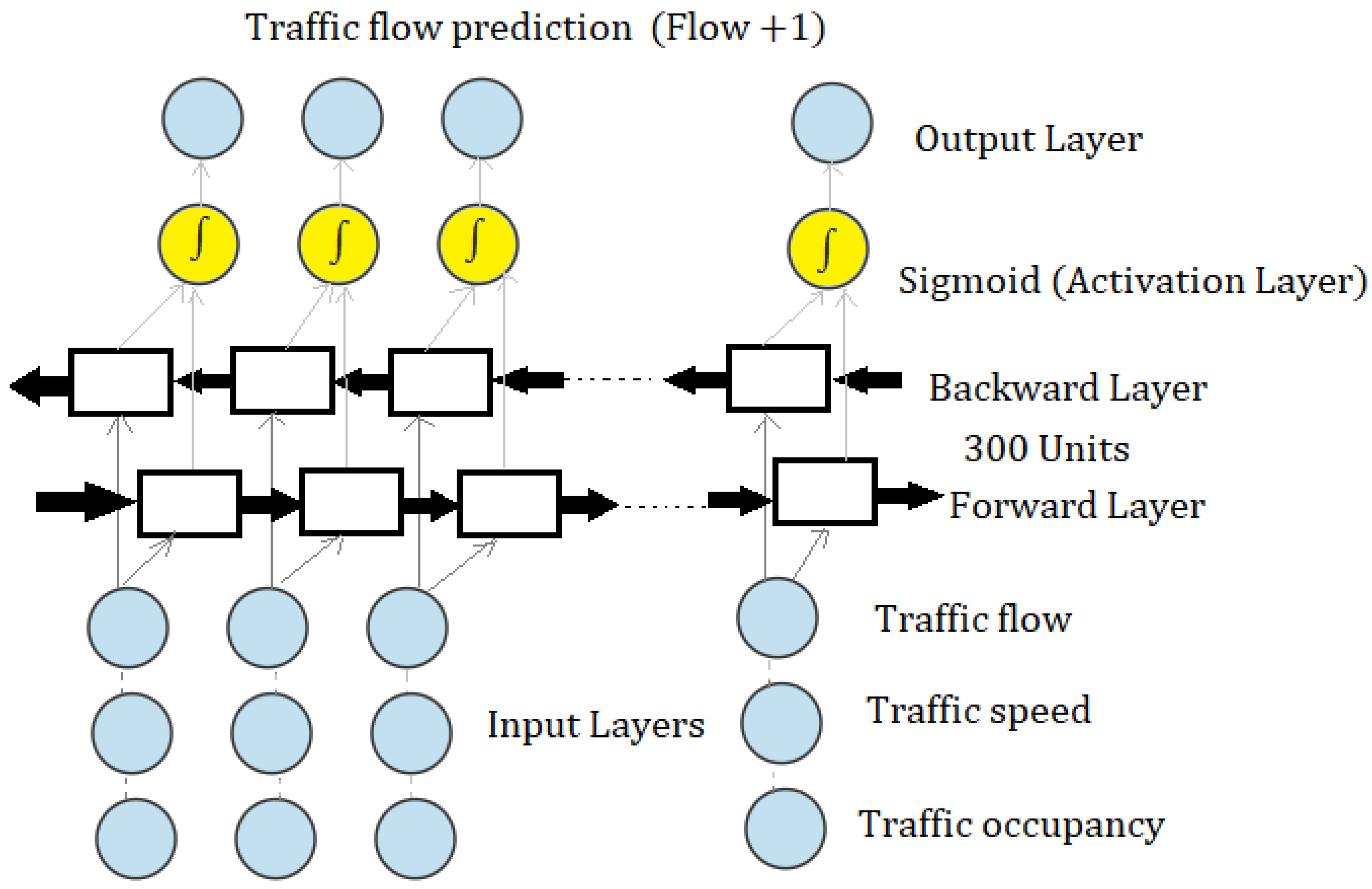
BiLSTM models expand upon a standard LSTM by processing input data in both forward and backward directions. This approach allows the model to capture relationships from both past and future data, offering a more comprehensive understanding of sequential information (see Figure 4).

The BiLSTM architecture captures temporal–spatial dependencies in sequential data through its internal memory cells and gating mechanisms, which are specifically designed to retain both short-term and long-term patterns. Each LSTM unit uses three gates, the input gate, forget gate, and output gate to regulate the flow of information, allowing the model to decide what new information to store (e.g., recurring peak-hour patterns), what past information to forget (discarding irrelevant noise), and what to output at each time step. This enables the model to maintain relevant long-term trends, such as recurring congestion patterns, while also responding to short-term fluctuations like sudden changes in traffic flow. The bidirectional structure further enhances this capability by processing the sequence in both forward and backward directions during training, providing the model with full temporal–spatial context. The chosen hyperparameters and training strategies play a crucial role in enhancing the BiLSTM model’s ability to learn complex temporal and spatial traffic patterns effectively. A minimum batch size of 128 balances computational efficiency and stable gradient estimation, enabling the model to generalise better across varied traffic conditions. Setting the maximum epochs to 300 allows sufficient training iterations for the model to converge and capture long-term dependencies without overfitting. The use of the Adaptive Moment Estimation (Adam) optimiser helps accelerate convergence by adaptively adjusting learning rates for each parameter, improving the model’s capacity to learn from noisy and complex traffic data. Incorporating a piecewise learning rate schedule with a drop period of 125 epochs and a drop factor of 0.2 gradually reduces the learning rate during training, which stabilises learning by allowing larger initial updates for faster convergence and smaller updates later to fine-tune the model. In addition, the number of hidden units (e.g., 300 in our model) controls the capacity to capture complex features, while the learning rate (e.g., 0.005) guides how effectively the model updates during training. Together, these factors optimise the training process, enabling the BiLSTM to more accurately model the intricate temporal sequences and spatial correlations inherent in multi-source traffic flow data, leading to improved prediction performance. Through these mechanisms, the BiLSTM effectively identifies patterns and dependencies in both time and space, which are critical for accurate traffic flow prediction.

6. Experiment 1

6.1. Variable Inputs Testing

In the first experiment, various combinations of flow (veh/h), speed (km/h), and occupancy (%) were tested for all the detectors for 5 min prediction horizons into the future. First, flow was trained and tested as the only input in the BiLSTM model, followed by (speed and flow), (occupancy and flow), and (speed, flow, and occupancy) as the inputs to the BiLSTM model in the variable inputs testing experiment. A representation of the model is provided in Figure 5. This results in four combinations (C1, C2, C3, and C4) as summarised in

Table 2. Various flow, speed, and occupancy combinations for eastbound and westbound directions.

Combinations	Flow (veh/h)	Speed (km/h)	Occupancy (%)
C1
C2
C3
C4

Note: Orange circles represent the variable inputs included in each combination.

below. The total number of data points used for model development is 216,084 observations for the speed, flow, and occupancy for each detector in the eastbound direction (1,512,588 for all detectors). The total number of observations in the westbound direction for speed, flow, and occupancy for each detector is 143,685 (1,005,795 for all detectors). The detector station WE4 is the main targeted eastbound detector for traffic flow prediction. WE1, WE2, and WE3 are the upstream detectors, and WE5, WE6, and WE7 are the downstream detectors. For the westbound direction, EW4 is the main targeted detector for traffic flow prediction. EW1, EW2, and EW3 are the downstream detectors, and EW5, EW6, and EW7 are the upstream detectors.

In order to develop the BiLSTM model, 60% of the data was used for training (129,650 observations), and 40% of the data was used for the testing and validation (86,434 observations) for each traffic feature (speed, flow, and occupancy). The mean absolute percentage error (MAPE) is employed to assess the accuracy of model predictions across various time horizons. It computes the average of the absolute differences between the predicted values (Y1) and the actual observed values (Y), expressed as a percentage:

$$\mathrm{MAPE} \mathrm{the} (\%)=({\displaystyle \frac{1}{n}}{\sum }_{i=1}^n{\displaystyle \frac{|Y-Y1|}{Y}})\ast 100$$

(7)

$$\mathrm{Accuracy} (\%)=(100 - \mathrm{MAPE})$$

(8)

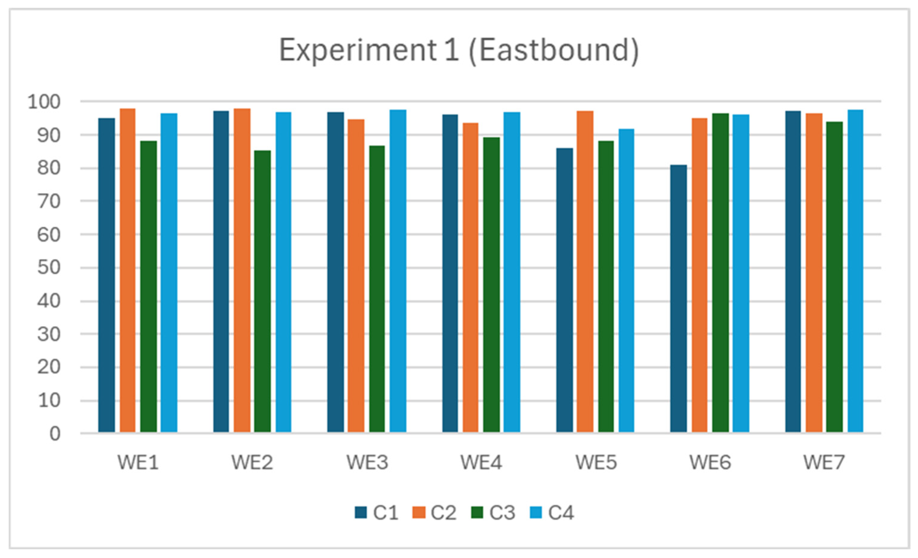
6.2. Experiment 1 Results (Eastbound)

The results of the four input combinations are presented in

Table 3. Performance of different input variable combinations for flow prediction accuracies for the seven detectors (eastbound direction).

Directions	Detectors	Accuracy (%) per Combination
		C1	C2	C3	C4
Eastbound	WE1	95.22	97.82	88.31	96.63
	WE2	97.37	97.93	85.18	96.89
	WE3	96.77	94.60	86.74	97.68
	WE4	96.01	93.59	89.12	96.80
	WE5	86.19	97.08	88.27	91.78
	WE6	81.05	95.14	96.48	96.20
	WE7	97.29	96.38	93.94	97.69

Note: The green cells represent the best-performing models, while the yellow cells represent the worst-performing models.

, showing that adding speed and occupancy as inputs generally improves flow prediction accuracy across all eastbound detectors.

For WE1 and WE2, the highest accuracies are achieved when speed is added to the flow input (C2: 97.82% and 97.93%, respectively), while using occupancy alone (C3) results in the lowest accuracies. A similar pattern is seen with WE5, where the flow input alone yields 86.19% accuracy, but significantly improves to 97.08% with the addition of speed.

For detectors WE3 and WE4, the best performance is observed when both speed and occupancy are included alongside flow (C4), achieving 97.68% and 96.80%, respectively. Especially, WE3 sees a slight decrease in accuracy when only speed is added (C2), suggesting the complementary value of combining both additional inputs.

Detector WE6 starts with the lowest baseline (C1: 81.05%) but shows significant improvements across all combinations, with the highest performance recorded when only occupancy is added (C3: 96.48%), closely followed by the full combination (C4: 96.20%).

For WE7, while the flow-only model performs well (97.29%), adding both speed and occupancy (C4) slightly improves the result to 97.69%. C3 (occupancy only) again yields the lowest performance.

The best-performing combinations are shaded green in Table 3, while the lowest performances are highlighted in yellow.

Figure 6 compares the prediction accuracies for each of the seven eastbound detectors under the four input combinations (C1–C4). This visualisation highlights the consistent improvements observed with the inclusion of speed and occupancy, especially under C4.

6.3. Experiment 1 Results (Westbound)

The results for the seven westbound detectors are shown in

Table 4. Performance of different input variable combinations for westbound flow prediction accuracies.

Directions	Detectors	Accuracy (%) per Combination
		C1	C2	C3	C4
Westbound	EW1	90.81	96.10	94.99	96.60
	EW2	88.19	95.90	92.03	90.07
	EW3	93.19	97.36	96.43	96.11
	EW4	92.43	83.27	74.74	93.43
	EW5	90.96	96.49	96.15	96.52
	EW6	91.11	95.17	82.49	96.58
	EW7	95.92	96.85	90.73	97.54

Note: The green cells represent the best-performing models, while the yellow cells represent the worst-performing models.

. In most cases, adding one or more variables to the flow improves prediction accuracy.

EW1, EW3, EW5, EW6, and EW7 show consistent improvements when additional variables are added to the flow. The highest accuracies for EW1 (96.60%), EW5 (96.52%), EW6 (96.58%), and EW7 (97.54%) occur with all three variables (C4), while EW3 performs best with flow and speed only (C2: 97.36%).

In addition to that, EW2 and EW4 show more sensitivity to input selection. For EW2, adding speed alone (C2) yields the best performance (95.90%), whereas adding all three inputs (C4) slightly decreases accuracy to 90.07%. Similarly, for EW4, both speed and occupancy individually degrade performance (C2: 83.27%, C3: 74.74%), while the full combination (C4) slightly improves over the flow-only input (93.43% vs. 92.43%).

As in Table 3, the best-performing combinations are shaded green, and the worst-performing ones are in yellow.

A similar comparison for westbound detectors is shown in Figure 7. The visual clearly demonstrates the varying degrees of benefit from different input combinations across detectors, highlighting that while C4 often yields the best results, some detectors perform best under C2 or C3 due to site-specific traffic dynamics.

7. Experiment 2

7.1. Neighbouring Detector Impacts

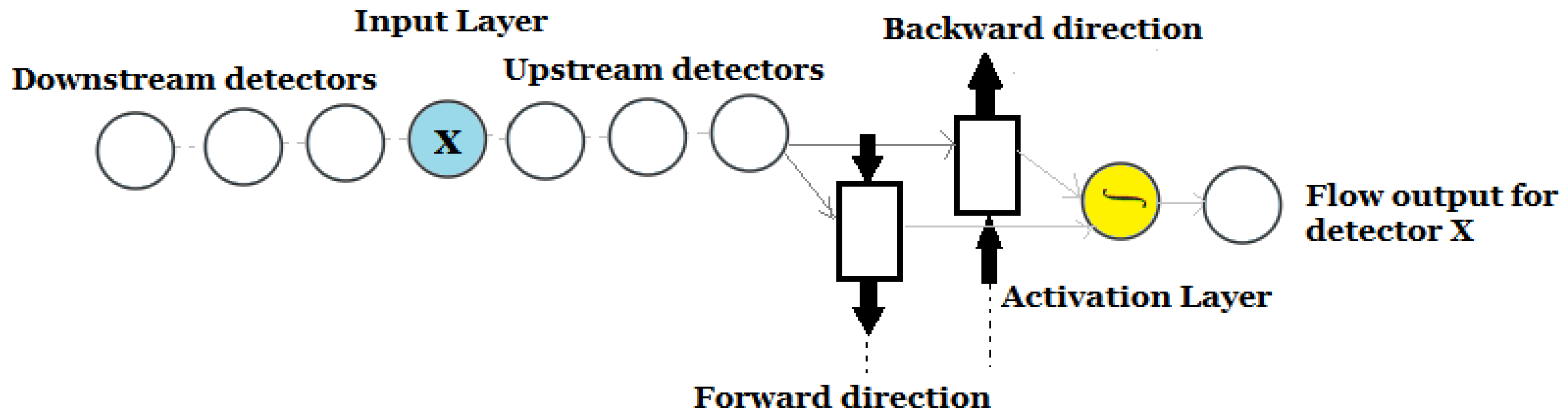
In this experiment, 32 short-term traffic BiLSTM models were trained and tested with different input settings in both the eastbound and westbound directions. The purpose is to test the impact of the upstream and downstream detectors on the flow prediction performance.

In this experiment, detectors WE4 (eastbound) and EW4 (westbound) were selected as the targeted detectors, and the improvement of flow prediction was investigated using the neighbouring detectors around those two targeted detectors. For the eastbound direction, the inputs of each BiLSTM model include the historical flow (veh/h) observations from the following detectors (WE1, WE2, WE3, WE4, WE5, WE6, and WE7). The expected output is the flow (veh/h) for the targeted detector WE4 at a prediction horizon of 5 min into the future.

For the westbound direction, the inputs of each BiLSTM model include the historical flow (veh/h) observations from the following detectors (EW1, EW2, EW3, EW4, EW5, EW6, and EW7). The expected output is the flow (veh/h) for the targeted detector EW4 at a prediction horizon of 5 min into the future. See Figure 8 below for the model illustration:

7.2. Experiment 2 Results (Eastbound)

The results of all model combinations are presented in

Table 5. Performance of neighbouring detectors on short-term traffic flow prediction for the eastbound direction.

Model	Eastbound Neighbouring Detector Inputs							Accuracy (%)
	WE1	WE2	WE3	WE4	WE5	WE6	WE7
1								96.01
2								96.84
3								98.16
4								96.66
5								97.32
6								97.26
7								97.67
8								94.32
9								96.07
10								97.57
11								97.06
12								97.70
13								96.48
14								98.22
15								97.45
16								96.35

Note: Orange circles represent the variable inputs included in each model. The green cells represent the best-performing model.

. These indicate that incorporating flow data from the neighbouring detectors generally improves short-term traffic flow prediction accuracy in the eastbound direction.

Starting with only the target detector WE4 (Model 1), the prediction accuracy was 96.01%. Adding downstream detectors progressively improved performance: WE3 alone (Model 2) increased accuracy to 96.84%, while WE2 and WE3 (Model 4) yielded 96.66%. Including three downstream detectors (WE1, WE2, and WE3 in Model 7) further improved accuracy to 97.67%.

Upstream inputs had an even stronger influence. Adding WE5 (Model 3) raised the accuracy significantly to 98.16%. Extending this to WE5 and WE6 (Model 6) produced 97.26%, and including WE7 as well (Model 14) gave the best result, 98.22%, marked in green in Table 5.

Mixed upstream and downstream combinations showed varying results. Models 5, 10, and 12, each including two upstream and two downstream detectors, produced accuracies of 97.32%, 97.57%, and 97.70%, respectively. However, not all combinations were beneficial: Model 8, using WE1–WE3 and WE5, resulted in a lower accuracy of 94.32%.

In general, models that included a balanced and broader range of upstream and downstream detectors tended to perform better. The poorest-performing model was Model 8 (94.32%), while the best-performing was Model 14 (98.22%).

7.3. Experiment 2 Results (Westbound)

The westbound prediction results, shown in

Table 6. Performance of neighbouring detectors on short-term traffic flow prediction for the westbound direction.

Model	Westbound Neighbouring Detector Inputs							Accuracy (%)
	EW1	EW2	EW3	EW4	EW5	EW6	EW7
1								92.43
2								93.81
3								96.23
4								96.77
5								95.80
6								95.43
7								94.99
8								94.18
9								97.12
10								97.32
11								94.82
12								94.62
13								96.32
14								96.73
15								96.11
16								96.43

Note: Orange circles represent the variable inputs included in each combination. The green cells represent the best-performing model.

, similarly demonstrate the value of including data from neighbouring detectors.

With only the target detector EW4 (Model 1), the prediction accuracy was 92.43%. Adding downstream detectors like EW3 (Model 2) improved it to 93.81%, while including both EW2 and EW3 (Model 4) raised it to 96.77%. Three downstream detectors (EW1, EW2, and EW3 in Model 7) achieved 94.99%.

Adding upstream detectors showed strong effects: WE5 alone (Model 3) improved accuracy to 96.23%, and the combination of WE5–WE6–WE7 (Model 10) reached the highest performance of 97.32%. This result is highlighted in green in Table 6.

Combinations of upstream and downstream detectors, such as in Models 9, 10, and 14, produced high accuracies ranging from 96.32% to 97.12%. As with the eastbound results, a broader input range managed to yield better accuracy, though not all combinations improved results equally. For example, Model 8, with upstream and downstream detectors, only reached 94.18%.

8. Relevance of Prediction Framework to the United Nations’ Sustainable Development Goals

The integration of machine learning for traffic flow prediction in urban transport management aligns strongly with the United Nations’ Sustainable Development Goals (SDGs). This study utilised the United Nations’ Sustainable Development Goals (SDGs) framework to analyse how each dimension of the proposed traffic flow prediction system, comprising advanced deep learning models, multisource data integration, and practical urban transport applications, relates to broader urban sustainability challenges. The SDGs were selected for their comprehensive global vision, integrative structure, and institutional relevance among various frameworks (such as the New Urban Agenda or the Global Sustainable Mobility Initiative). The SDGs’ focus on sustainable cities, climate-responsive planning, and infrastructure innovation aligns directly with the research problem addressed in this study. The proposed research contributes directly and indirectly to several SDG targets related to sustainable infrastructure, climate resilience, and inclusive mobility through the application of advanced deep learning models such as LSTM and BiLSTM, combined with multisource data fusion and environmental consideration.

Following a critical review of traffic forecasting literature, urban mobility strategies, and smart city applications, the authors examined how the elements of the proposed prediction framework map onto specific SDG targets.

Table 7. Linkage of machine learning traffic flow prediction to the UN’s Sustainable Development Goals (SDGs).

Framework Components	Directly Connected SDG Targets	Indirectly Connected
Methodological Approach	9.1—Develop quality, reliable, sustainable, and resilient infrastructure for supporting economic development and human well-being, with a focus on affordable and equitable access for all	4.7—Ensure learners acquire knowledge and skills to promote sustainable development
	11.2—Provide access to safe, affordable, accessible, and sustainable transport systems for all	10.7—Facilitate orderly, safe, regular and responsible migration and mobility of people
	13.2—Integrate climate change measures into national policies, strategies, and planning	17.6—Enhance access to science, technology, and innovation
Multisource Data Integration	17.18—Enhance capacity-building support to developing countries to increase the availability of high-quality, timely, and reliable data	12.8—Ensure that people everywhere have relevant information and awareness for sustainable development and lifestyles
	11.6—Reduce the adverse per capita environmental impact of cities, including by paying special attention to air quality and municipal and other waste management	13.3—Improve education and awareness on climate change; build capacity for climate-related planning
Advanced Model Development (BiLSTM)	9.5—Enhance scientific research and upgrade technological capabilities of industrial sectors in developing countries	8.4—Improve progressively, through 2030, global resource efficiency in consumption and production
	11.3—Enhance inclusive and sustainable urbanisation and capacity for participatory, integrated and sustainable human settlement planning and management	1.5—Build resilience of people with low incomes and those in vulnerable situations, and reduce exposure to climate-related extreme events
Impact on Urban Traffic Management	13.2—Integrate climate change measures into national policies, strategies, and planning	3.9—Substantially reduce the number of deaths and illnesses from air pollution
	3.6—Halve the number of global deaths and injuries from road traffic accidents	12.2—Achieve sustainable management and efficient use of natural resources
	11.2—Provide access to safe, affordable, accessible, and sustainable transport systems for all	16.7—Ensure responsive, inclusive, participatory, and representative decision-making
Sustainable Mobility Contributions	13.2—Integrate environmental concerns into planning and operations	16.7—Ensure inclusive and participatory decision-making
	9.1—Develop quality, reliable, sustainable infrastructure	12.4—Reduce release of hazardous substances
	11.6—Minimise negative environmental impacts from urban traffic	11. a—Link urban–rural development planning

Table source: Author developed based on publicly available SDG data [60,61,62,63,64,65,66,67,68,69,70,71].

maps the core dimensions of the traffic flow prediction approach, including methodological design, data integration, model innovation, and expected outcomes, to specific SDGs. These targets include direct connections such as those related to transport safety (SDG 3.6), sustainable infrastructure (SDG 9.1), inclusive access (SDG 11.2), and climate-responsive policy integration (SDG 13.2). Indirect contributions are also evident, such as enhancing awareness (SDG 12.8), enabling inclusive decision-making (SDG 16.7), and promoting technological capacity (SDG 17.6). Table 7 systematically maps how each core component of the proposed traffic flow prediction system contributes to relevant SDG targets, highlighting specific mechanisms of impact.

Figure 9 visualises these cross-dimensional relationships, highlighting both strong direct (solid lines) and broader indirect (dotted lines) alignments with key SDG targets. This alignment reaffirms the model’s value as a tool for operational efficiency in transport and as a strategy for equitable, resilient, and low-emission urban futures. Figure 9 visualises these connections, highlighting both the strong direct relationships (solid lines) and broader indirect associations (dotted lines) between the traffic flow prediction framework and various SDGs. The strongest alignment was observed with SDG 11 (sustainable cities), SDG 9 (infrastructure), SDG 13 (climate action), and SDG 17 (technology and governance), with supporting roles for SDG 3 (health), SDG 12 (responsible consumption), and others.

This alignment underscores that AI-driven traffic flow prediction is a tool for enhancing operational transport efficiency and a strategic enabler of equitable, low-emission, and resilient urban futures. However, it should be noted that similar to the findings by Brussel et al. [72], current SDG indicators may underrepresent the complexity of real-world transport accessibility and behavioural patterns. Despite this, the SDG framework remains a valuable reference point for aligning transport innovations with global policy and sustainability discourse.

9. Discussion of Results

The above results demonstrate that multisource traffic data inputs, such as occupancy, flow, and speed from the same detector, can improve the accuracy of the flow prediction model. For the westbound direction, the accuracy improvement ranges from 1% to 6% for all detectors. It can also be noted that adding speed, occupancy, and flow together as inputs improves the accuracy of the five westbound detectors. The remaining two detectors achieved the highest accuracy when speed and flow were tested together as inputs to the model. Moreover, adding occupancy to the flow alone has the lowest improvement to model performance for most detectors in both travel directions. Overall, the accuracy improvement reaches up to 15% for all detectors in the eastbound direction.

In the westbound direction, it can also be noted that adding (speed, occupancy, and flow) or (speed and flow) together as inputs improved the accuracy of six detectors. The remaining detector achieved the highest accuracy when speed and occupancy were tested together as inputs to the model. However, adding occupancy to the remaining six detectors has resulted in the lowest improvement to the model performance in general.

In addition, the results above demonstrate that multisource traffic flow data input from the neighbouring detectors improved the accuracy of the flow prediction model. The accuracy improvement ranges from 1% to 5% for the westbound direction. The most significant improvement was achieved when flow data from three neighbouring detectors upstream was added, with an accuracy of 97.32% compared to 92.42% when the flow was predicted from a single detector flow input.

The accuracy improved by around 2% for the eastbound direction by using traffic flow data from the adjacent detectors. The most significant improvement resulted when flow data from two neighbouring detectors upstream and three neighbouring detectors downstream was added, with an accuracy of 98.99% compared to 96.01% when the flow was predicted from a single detector flow input.

The results demonstrate that the most accurate flow predictions are obtained when speed, flow, and occupancy inputs are used from the same detector to train the model. Excluding the speed or occupancy from the inputs leads to a deterioration in flow prediction performance. The results also demonstrate the direct influence of using additional inputs from upstream detector stations and show that, generally, these additional inputs result in better prediction accuracies.

These findings validate the effectiveness of incorporating multiple features and spatially distributed data in traffic flow prediction and carry significant implications for sustainable urban transport development. The improved accuracy in predicting flow can contribute to more efficient traffic control, reduced congestion, and better utilisation of existing infrastructure, aligning directly with Sustainable Development Goal (SDG) 9.1, which promotes reliable and sustainable infrastructure.

From a broader sustainability perspective, the following applies:

• The enhancement of prediction accuracy using multisource and spatial data supports the development of intelligent transport systems, which are important for SDG 11.2 (providing access to safe, affordable, and sustainable transport systems for all).
• More accurate flow predictions also enable traffic management systems to proactively adjust control measures, reduce emissions from congestion, and promote fuel efficiency, supporting SDG 13.2, for climate-related planning and the reduction of greenhouse gas emissions.
• Indirectly, these improvements can reduce exposure to traffic-related air pollution, contributing to SDG 3.9 (reducing illnesses from hazardous air and environmental pollution), and enhance safety by anticipating congestion-related incidents in support of SDG 3.6 (reducing the number of global deaths and injuries from road traffic accidents).
• Finally, integrating such high-quality, granular data into model development aligns with SDG 17.18, highlighting the importance of timely, reliable, and disaggregated data for decision-making.

In summary, the observed improvements in prediction accuracy, whether through data variety (speed, flow, occupancy) or spatial diversity (input from upstream/downstream detectors), highlight the potential of advanced machine learning models to support technical transport outcomes and broader sustainability goals.

Practical Implications and Limitations

The results presented in this study demonstrate the potential of incorporating multisource and spatially distributed traffic data to improve short-term flow prediction accuracy using BiLSTM models significantly. The practical implementation of such models in real-world traffic management systems needs further discussion.

The enhanced accuracy of flow predictions offers substantial benefits for existing traffic management practices. For example, integrating adaptive traffic signal control systems could enable dynamic optimisation of signal timings based on predicted demand, reducing congestion and making for more efficient use of road infrastructure. Similarly, predictive outputs from the model could inform real-time traveller information systems, allowing road users to receive early warnings about potential delays and make informed route or departure time decisions. Short-term flow predictions can also support incident management by detecting irregular traffic patterns earlier than traditional threshold-based methods, enabling immediate operator response.

However, transitioning from experimental study to operational use involves several challenges. Real-time performance is essential; the model must deliver predictions with minimal errors. This requires efficient data preprocessing pipelines and computationally lightweight inference procedures to be implemented in parallel with existing control systems. Moreover, the reliability of input data plays a central role in maintaining prediction accuracy. Incomplete or noisy data from traffic detectors can worsen the quality of model outputs; therefore, data cleaning methods are necessary as part of the operational framework.

Another key issue is the adaptability of the model over time. A wide range of dynamic factors, such as seasonal trends, roadworks, and changes in demand, influence traffic patterns. Therefore, periodic retraining of the model using up-to-date data is essential to maintain its accuracy in a continuously evolving traffic environment. Future development could explore real-time learning approaches or feedback mechanisms that enable an incremental model updating without full retraining.

Future work should include collaboration with transport agencies to pilot the model in operational settings, assess scalability, and ensure integration into existing traffic management platforms. Such partnerships will help bridge the gap between model development and practical deployment, improving the advantage of predictive models in real-world scenarios.

10. Conclusions

This study has demonstrated the effectiveness of using multisource traffic data inputs to improve short-term traffic flow prediction accuracy, a key aspect of sustainable traffic management. By incorporating occupancy, flow, and speed data from individual detectors, the prediction accuracy improved significantly for both eastbound and westbound directions. The results indicate that integrating multiple input variables enhances model performance, particularly for specific input combinations. In the westbound direction, accuracy improvements between 1% and 6% were observed for all detectors, with the most substantial improvements achieved when speed, occupancy, and flow were combined. Significantly, five westbound detectors showed improved accuracy with this combination, while two other stations reached optimal accuracy when speed and flow were used without occupancy. On the other hand, adding only occupancy to flow produced minimal improvements, highlighting that the combined use of speed and flow is particularly valuable for accurate traffic flow predictions in the westbound direction.

In the eastbound direction, the findings show that incorporating occupancy, speed, and flow yields an accuracy improvement of up to 15% across all detectors, underscoring the benefit of using multisource data inputs. Similarly, spatial input interactions from neighbouring detectors were found to be beneficial, especially for predicting westbound traffic flows, where incorporating data from three upstream detectors improved accuracy from 92.42% to 97.32%. For the eastbound direction, leveraging data from two upstream and three downstream neighbouring detectors boosted accuracy to 98.99%, compared to 96.01% when using single-detector input.

In summary, this study emphasises the effectiveness of multisource data and spatial interactions for enhancing traffic flow predictions in both travel directions. By identifying optimal input configurations, mainly through the inclusion of speed and occupancy, this research offers a valuable approach for refining short-term traffic prediction models. The study also highlights the value of machine learning and multi-source data integration in reducing congestion, lowering emissions, and improving mobility, contributing to developing sustainable, data-driven traffic management systems. This research supports future strategies for intelligent transportation systems that encourage efficient, environmentally friendly, and resilient road networks, aligning with the sustainability goals for urban mobility.

Additionally, the study incorporated a Sustainable Development Goals (SDGs) analysis, highlighting how improved traffic flow predictions contribute to SDG 9 (infrastructure), SDG 11 (sustainable cities), SDG 13 (climate action), and others, emphasising the broader societal and environmental relevance of data-driven transport modelling.